Parametric Copula-GP model for analyzing multidimensional neuronal and behavioral relationships

Abstract

One of the main challenges in current systems neuroscience is the analysis of high-dimensional neuronal and behavioral data that are characterized by different statistics and timescales of the recorded variables. We propose a parametric copula model which separates the statistics of the individual variables from their dependence structure, and escapes the curse of dimensionality by using vine copula constructions. We use a Bayesian framework with Gaussian Process (GP) priors over copula parameters, conditioned on a continuous task-related variable. We validate the model on synthetic data and compare its performance in estimating mutual information against the commonly used non-parametric algorithms. Our model provides accurate information estimates when the dependencies in the data match the parametric copulas used in our framework. When the exact density estimation with a parametric model is not possible, our Copula-GP model is still able to provide reasonable information estimates, close to the ground truth and comparable to those obtained with a neural network estimator. Finally, we apply our framework to real neuronal and behavioral recordings obtained in awake mice. We demonstrate the ability of our framework to 1) produce accurate and interpretable bivariate models for the analysis of inter-neuronal noise correlations or behavioral modulations; 2) expand to more than 100 dimensions and measure information content in the whole-population statistics. These results demonstrate that the Copula-GP framework is particularly useful for the analysis of complex multidimensional relationships between neuronal, sensory and behavioral data.

1 Introduction

Recent advances in imaging and recording techniques have enabled monitoring the activity of hundreds to several thousands of neurons simultaneously [1, 2, 3]. These recordings can be made in awake animals engaged in specifically designed tasks or natural behavior [4, 5, 6], which further augments these already large datasets with a variety of behavioral variables. These complex high dimensional datasets necessitate the development of novel analytical approaches [7, 8, 9, 10] to address two central questions of systems and behavioral neuroscience: how do populations of neurons encode information? And how does this neuronal activity correspond to the observed behavior? In machine learning terms, both of these questions translate into understanding the high-dimensional multivariate dependencies between the recorded variables [11, 12, 13, 14].

There are two major methods suitable for recording the activity of large populations of neurons from behaving animals: the multi-electrode probes that provide milliseconds precision for recordings of electrical activity [1], and calcium imaging methods [2, 3, 15] that use changes in intracellular calcium concentration as a proxy for neuronal spiking activity at a lower (tens of milliseconds) temporal precision. As a result, the recorded neuronal and behavioral variables may operate at different timescales and exhibit different statistics, which further complicates the statistical analysis.

The natural approach to modeling statistical dependencies between the variables with drastically different statistics is based on copulas, which separate marginal statistics from the dependence structure [16]. For this reason, copula models are particularly effective for mutual information estimation [17, 18]. They can also escape the ‘curse of dimensionality’ by factorising the multi-dimensional dependence into pair-copula constructions called vines [19, 20]. Copula models have been successfully applied to spiking activity [21, 22, 23, 24], 2-photon calcium recordings [25] and multi-modal neuronal datasets [26]. However, these models assumed that the dependence between variables was static, whereas in neuronal recordings it may be dynamic or modulated by behavioral context [27, 14]. Therefore, it might be helpful to explicitly model the continuous time- or context-dependent changes in the relationships between variables, which reflect changes in an underlying computation.

Here, we extend a copula-based approach by adding explicit conditional dependence to the parameters of the copula model, approximating these latent dependencies with Gaussian Processes (GP). It was previously shown that such a combination of parametric copula models with GP priors outperforms static copula models [28] and even dynamic copula models on many real-world datasets, including weather forecasts, geological data or stock market data [29]. Yet, this method has never been applied to neuronal recordings before.

In this work, we improve the scalability of the method by using stochastic variational inference. We also increase the complexity of the copula models in order to adequately describe the complex dependencies commonly observed in neuronal data. In particular, we use mixtures of parametric copula models to account for changes in tail dependencies. We develop model selection algorithms, based on the fully-Bayesian Watanabe–Akaike information criterion (WAIC). Finally and most importantly, we demonstrate that our model is suitable for estimating mutual information. It performs especially well when the parametric model can closely approximate the target distribution. When it is not the case, our copula mixture model demonstrates sufficient flexibility and provides close information estimates, comparable to the best state-of-the-art non-parametric information estimators.

We first introduce the copula mixture models and propose model selection algorithms (Sec. 2). We then validate our model on synthetic data and compare its performance against other commonly used information estimators (Sec. 3). Next, we demonstrate the utility of the method on real neuronal and behavioral data (Sec. 4). We show that our Copula-GP method can produce interpretable bivariate models that emphasize the qualitative changes in tail dependencies and estimate mutual information that exposes the structure of the task without providing any explicit cues to the model. Finally, we apply the vine Copula-GP model to measure information content in the whole dataset with 5 behavioral variables and more than 100 neurons.

2 Parametric copula mixtures with Gaussian process priors

Our model is based on copulas: multivariate distributions with uniform marginals. Sklar’s theorem [30] states that any multivariate joint distribution can be written in terms of univariate marginal distribution functions $p(Y_{i})$ and a unique copula which characterizes the dependence structure: $p(Y_{1},\ldots,Y_{N})=c(F_{1}(Y_{1})\ldots F_{N}(Y_{N}))\times\prod_{i=1}^{N}p(Y_{i})$. Here, $F_{i}(\cdot)$ are the marginal cumulative distribution functions (CDF) and, as a result, each $F_{i}(Y_{i})$ is uniformly distributed on [0,1].

For high dimensional datasets (high $\mathrm{dim}\mathbf{Y}$), maximum likelihood estimation for copula parameters may become computationally challenging. The two-stage inference for margins (IFM) training scheme is typically used in this case [31]. First, univariate marginals are estimated and used to map the data onto a multidimensional unit cube. Second, the parameters of the copula model are inferred.

Conditional copulas

Following the approach by Hernández-Lobato et al. [29], we are using Gaussian Processes (GP) to model the conditional dependencies of copula parameters:

$$p(\mathbf{Y}|X)=c\Big{(}F_{1}(Y_{1}|X),\ldots,F_{N}(Y_{N}|X)\Big{|}X\Big{)}\times\left[\prod_{i=1}^{N}p(Y_{i}|X)\right].$$ (1)

In the most general case, the marginal PDFs $p(Y_{i}|X)$ and CDFs $F_{i}(Y_{i}|X)$ and the copula $c(\ldots|X)$ itself can all be conditioned on $X$. In our framework, $X$ is assumed to be one-dimensional. A Gaussian Process is ideally suited for copula parametrization, as it provides an estimate of the uncertainty in model parameters, which we utilize in our model selection process (Sec. 2.1).

Conditional marginals

In order to estimate marginal CDFs $F(Y_{i}|X)$, we use the non-parametric fastKDE [32] algorithm, which allows for direct estimation of the conditional distributions. The conditional distribution is then used to map the data onto a unit hypercube using the probability integral transform: $F(Y_{i}|X)\rightarrow U_{i}\sim U_{[0,1]}$, such that $U_{i}$ is uniformly distributed for any $X$.

Bivariate copula families

We use 4 copula families as the building blocks for our copula models: Gaussian, Frank, Clayton and Gumbel copulas (Figure 1). All of these families have a single parameter, corresponding to the rank correlation (Table 1). We also use rotated variants (90^∘, 180^∘, 270^∘) of Clayton and Gumbel copula families in order to express upper tail dependencies and negative correlation.

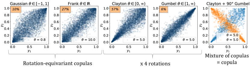
Figure 1: Copula families used in the mixture models in our framework. The percentage in the upper-left corner shows how often each of the families was selected to be used in a copula mixture for pairwise relationships in the real neuronal data from Pakan et al. [5] (see Sec. 4).

Table 1: Bivariate copula families and their GPLink functions

Copula	Domain	$\mathrm{GPLink}(f):\mathbb{R}\rightarrow\mathop{\mathrm{dom}}(c_{j})$
Independence	–	–
Gaussian	[-1,1]	$\mathrm{Erf}(f/1.4)$
Frank	(-$\infty$, $\infty$)	$0.3\cdot f+\mathrm{sign}(f)\cdot(0.3\cdot f)^{2}$
Clayton	[0,$\infty$)	$\mathrm{Exp}(0.3\cdot f)$
Gumbel	[1,$\infty$)	$1+\mathrm{Exp}(0.3\cdot f)$

Since we are primarily focused on the analysis of neuronal data, we have first visualized the dependencies in calcium signal recordings after a probability integral transform, yielding empirical conditional copulas. As a distinct feature in neuronal datasets, we observed changes in tail dependencies with regard to the conditioning variable. Since none of the aforementioned families alone could describe such conditional dependency, we combined multiple copulas into a linear mixture model (which is also a copula [33]):

$$c\left(\mathbf{U}\middle|X\right)=\sum_{j=1}^{K}\phi_{j}(X)c_{j}(\mathbf{U};\theta_{j}(X)),$$ (2)

where $K$ is the number of elements, $\phi_{j}(X)$ is the concentration of the $j$th copula in a mixture, $c_{j}$ is the pdf of the $j$th copula, and $\theta_{j}$ is its parameter.

Each of the copula families includes the Independence copula as a special case. To resolve this overcompleteness, we add the Independence copula as a separate model with zero parameters (Table 1). For independent variables $\mathbf{Y}_{ind}$, the Independence model will be preferred over the other models in our model selection algorithm (Sec. 2.1), since it has the smallest number of parameters.

Gaussian Process priors

We parametrize the mixture model (2) with the independent latent GPs: $\mathbf{f}\sim\mathcal{N}(\mu\times\mathbf{1},K_{\lambda}(X,X))$. For each copula family, we constructed GPLink functions (Table 1) that map the GP variable onto the copula parameter domain: $\theta_{j}=\mathrm{GPlink}_{c_{j}}(f_{j}),\mathbb{R}\rightarrow\mathop{\mathrm{dom}}(c_{j}).$ Next, we also use GP to parametrize concentrations $\phi_{j}(X)$, which are defined on a simplex ($\sum\phi=1$):

$$\phi_{j}=(1-t_{j})\prod_{m=1}^{j-1}t_{m},\quad t_{m}=\Phi\left(\widetilde{f}_{m}+\Phi^{-1}\left(\frac{M-m-1}{M-m}\right)\right),\quad t_{M}=0,$$

where $\Phi$ is a CDF of a standard normal distribution and $\mathbf{\widetilde{f}_{m}}\sim\mathcal{N}(\widetilde{\mu}_{m}\times\mathbf{1},\widetilde{K}_{\widetilde{\lambda}_{m}}(X,X))$. This parametrization ensures that when all GP variables $\widetilde{f}_{m}=0$, all of the concentrations $\phi_{j}$ are equal to $1/M$. We use the RBF kernel $K_{\lambda}(X,X)$ with bandwidth parameter $\lambda$. Therefore, the whole mixture model with $M$ copula elements requires $[2M-1]$ hyperparameters: $\{\lambda\}_{M}$ for $\bm{\theta}$ and $\{\widetilde{\lambda}\}_{M-1}$ for $\bm{\phi}$.

Approximate Inference

Since our model has latent variables with GP priors and intractable posterior distribution, the direct maximum likelihood Type-II estimation is not possible and an approximate inference is needed. Such inference problem with copula models has previously been solved with the expectation propagation (EP) algorithm [29]. Considering the recent developments in high-performance parallel computing and stochastic optimization algorithms, we chose to use stochastic variational inference (SVI) instead. In order to scale the SVI to a large number of inputs, we use Kernel Interpolation for Scalable Structured Gaussian Processes (KISS-GP) [34]. For efficient implementation of these methods on GPU, we use the PyTorch [35] and GPyTorch libraries [36].

2.1 Bayesian Model selection

We use the Watanabe–Akaike information criterion (WAIC [37]) for model selection. WAIC is a fully Bayesian approach to estimating the Akaike information criterion (AIC) (see Eq. 31 in the original paper [37]). The main advantage of the method is that it avoids the empirical estimation of the effective number of parameters, which is often used for approximation of the out-of-sample bias. It starts with the estimation of the log pointwise posterior predictive density (lppd) [38]:

$$\widehat{\mathrm{lppd}}=\sum_{i=1}^{N}\log\left(\frac{1}{S}\sum_{s=1}^{S}p(y_{i}|\theta^{s})\right),\qquad p_{\mathrm{WAIC}}=\sum_{i=1}^{N}V_{s=1}^{S}\Big{(}\log p(y_{i}|\theta^{s})\Big{)},$$

where $\{\theta^{s}\}_{S}$ is a draw from a posterior distribution, which must be large enough to represent the posterior. Next, the $p_{\mathrm{WAIC}}$ approximates the bias correction, where $V_{s=1}^{S}$ represents sample variance. Therefore, the bias-corrected estimate of the log pointwise posterior predictive density is given by: $e\widehat{\mathrm{lppd}}_{\mathrm{WAIC}}=\mathrm{lppd}-p_{\mathrm{WAIC}}=-N\cdot{\mathrm{WAIC}_{original}}.$

In the model selection process, we aim to choose the model with the lowest $\mathrm{WAIC}$. Since our copula probability densities are continuous, their values can exceed 1 and the resulting $\mathrm{WAIC}$ is typically negative. Zero $\mathrm{WAIC}$ corresponds to the Independence model ($\mathrm{pdf}=1$ on the whole unit square).

Since the total number of combinations of 10 copula elements (Fig. 1, considering rotations) is large, exhaustive search for the optimal model is not feasible. In our framework, we propose two model algorithms for constructing close-to-optimal copula mixtures: greedy and heuristic (see Supplemental Material for details). The greedy algorithm is universal and can be used with any other copula families without adjustment, while the heuristic algorithm is fine-tuned to the specific copula families used in this paper (Fig. 1). Both model selection algorithms were able to select the correct 1- and 2-component model on simulated data and at least find a close approximation (within $\mathrm{WAIC}_{tol}=0.005$) for more complex models (see validation of model selection in Supplemental Material).

2.2 Entropy and mutual information

Our framework provides tools for efficient sampling from the conditional distribution and for calculating the probability density $p(\mathbf{Y}|X)$. Therefore, for each $X=x$ the entropy $H(\mathbf{Y}|X=x)$ can be estimated using Monte Carlo (MC) integration:

$$H(\mathbf{Y}|X=x)=-\mathop{\mathbb{E}}_{p(\mathbf{Y}|X=x)}\log p(\mathbf{Y}|X=x).$$ (3)

$p(\mathbf{Y}|X=x)$ factorizes into the conditional copula density and marginal densities (1), hence for each $x$ the entropy also factorizes [17] as $H(\mathbf{Y}|X=x)=\sum H(Y_{i}|X=x)+H_{c}(\mathbf{U}^{X}|X=x)$, where $\mathbf{U}^{X}=\mathbf{F}(\mathbf{Y}|X)$. The conditional entropy can be integrated as $H(\mathbf{Y}|X)=\sum_{i=1}^{N}H(Y_{i}|X)+\int H_{c}(\mathbf{U}^{X}|X=x)p(x)dx,$ separating the entropy of the marginals $\{Y_{i}\}_{N}$ from the copula entropy.

Now, $I(X,\mathbf{Y})=I(X,\mathbf{G(Y)})$ if $\mathbf{G(Y)}$ is 1) a homeomorphism, 2) independent of $X$ [39]. If marginal statistics are independent of $X$, then the probability integral transform $\mathbf{U}=\mathbf{F}(\mathbf{Y})$ satisfies both requirements, and $I(X,\mathbf{Y})=I(X,\mathbf{U})$. Then, in order to calculate the mutual information $I(X,\mathbf{U})\coloneqq H(\mathbf{U})-H(\mathbf{U}|X)$, we must also rewrite it using only the conditional distribution $p(\mathbf{U}|X)$, which is modelled with our conditional Copula-GP model. This can be done as follows:

$$I(X,\mathbf{U})=H(\mathbf{U})-\int H(\mathbf{U}|X=x)p(x)dx=\mathop{\mathbb{E}}_{p(\mathbf{U},X)}\log p(\mathbf{U}|X)-\mathop{\mathbb{E}}_{p(\mathbf{U})}\log\mathop{\mathbb{E}}_{p(X)}p(\mathbf{U}|X).$$ (4)

The last term in (4) involves nested integration, which is computationally difficult and does not scale well with $N=\mathrm{dim}\mathbf{U}$. Therefore, we propose an alternative way of estimating $I(X,\mathbf{Y})$, which avoids double integration and allows us to use the marginals conditioned on $X$ ($\mathbf{U}^{X}=\mathbf{F}(\mathbf{Y}|X)$), providing a better estimate of $H(\mathbf{Y}|X)$. We can use two separate copula models, one for estimating $p(\mathbf{Y})$ and calculating $H(\mathbf{Y})$, and another one for estimating $p(\mathbf{Y}|X)$ and calculating $H(\mathbf{Y}|X)$:

$$I(X,\mathbf{Y})=\sum_{i=1}^{N}I(X,Y_{i})+H_{c}{(u_{1},\ldots,u_{N})}-\int H_{c}(u^{x}_{1},\ldots,u^{x}_{N}|s=x)p(x)dx,$$ (5)

where both entropy terms are estimated with MC (3). Here we only integrate over the unit cube $[0,1]^{N}$ and then $\mathrm{dom}\,X$, whereas (4) required integration over $[0,1]^{N}\times\mathrm{dom}\,X$.

The performance of both (4) and (5) critically depends on the approximation of the dependence structure, i.e. how well the parametric copula approximates the true copula probability density. If the joint distribution $p(Y_{1}\ldots Y_{N})$ has a complex dependence structure, as we will see in synthetic examples, then the mixture of parametric copulas may provide a poor approximation of $p(\mathbf{Y})$ and overestimate $H_{c}{(u_{1},\ldots,u_{N})}$, thereby overestimating $I(X,\mathbf{Y})$. The direct integration (4), on the other hand, typically underestimates the $I(X,\mathbf{Y})$ due to imperfect approximation of $p(\mathbf{Y}|X)$, but it is only applicable if the marginals can be considered independent of $X$.

We further refer to the direct integration approach (4) as "Copula-GP integrated" and to the alternative approach (5) as "Copula-GP estimated" and assess both of them on synthetic and real data.

2.3 Copula vine constructions

High-dimensional copulas can be constructed from bivariate copulas by organizing them into hierarchical structures called copula vines [19]. In this paper, we focus on the canonical vine or C-vine, which factorizes the high-dimensional copula probability density function as follows:

$$c(\mathbf{U})=\left[\prod_{i=2}^{N}c_{1i}(U_{1},U_{i})\right]\times\left[\prod_{i=2}^{N}\prod_{j=i+1}^{N}c_{ij|\{k\}_{k<i}}\left(F(U_{i}|\{U_{k}\}_{k<i}),F(U_{j}|\{U_{k}\}_{k<i})\right)\right]$$ (6)

where $\{k\}_{k<i}=1,\ldots,i-1$, $\{U_{k}\}_{k<i}=U_{1},\ldots,U_{i-1}$ and $F(U_{i}|\{U_{k}\}_{k<i})$ is a conditional CDF. Note, that all of the copulas in (6) can also be conditioned on $X$ via Copula-GP model. We choose the first variable $U_{1}$ to be the one with the highest rank correlation with the rest (sum of absolute values of pairwise Kendall’s $\tau$), and condition all variables on the first one. We repeat the procedure until no variable is left. It was shown by Czado et al. [40] that this ordering facilitates C-vine modeling.

Code availability

Code will be made available on GitHub upon paper acceptance.

3 Validation on artificial data

We compare our method with the other commonly used non-parametric algorithms for mutual information estimation: Kraskov-Stögbauer-Grassberger (KSG [39]), Bias-Improved-KSG by Gao et al. (BI-KSG [41]) and the Mutual Information Neural Estimator (MINE [42]).

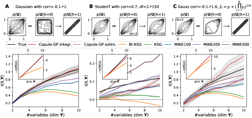
Figure 2: Conditional entropy $H(\mathbf{Y}|X)$ and mutual information $I(X,\mathbf{Y})$ measured by different methods on synthetic data. Upper row shows the dependency structures $p(\mathbf{U})$ and conditional dependency structures at the beginning and the end of the $\textrm{dom}X=[0,1]$. A  Multivariate Gaussian samples. B  Multivariate Student T samples. C  Multivariate Gaussian samples $\mathbf{Y}$ (same as A), morphed into another distribution $p(\hat{\mathbf{Y}})$ with a tail dependence, while $I(X,\mathbf{Y})=I(X,\hat{\mathbf{Y}})$. Gray intervals show either standard error of mean (SE, 5 repetitions), or $\sqrt{(SE)^{2}+(MC_{tol})^{2}}$ for integrated variables.

First, we test these estimators on a dataset sampled from a multivariate Gaussian distribution, with $\mathrm{cov}(Y_{i},Y_{j})=\rho+(1-\rho)\,\delta_{ij}$, where $\delta_{ij}$ is Kronecker’s delta and $\rho=-0.1+1.1X,X~{}\in~{}[0,1]$. Our algorithm selects a Gaussian copula on these data, which perfectly matches the true distribution. Therefore, Copula-GP measures both entropy and mutual information exactly (within integration tolerance, see Fig. 2A). The performance of the non-parametric methods on this dataset is lower. It was shown before that KSG and MINE both severely underestimate the $\mathrm{MI}$ for high-dimensional Gaussians with high correlation (e.g. see Fig. 1 in Belghazi et al. [42]). The Copula-GP model (integrated) provides accurate estimates for highly correlated (up to $\rho=0.999$, at least up to 20D) Gaussian distributions (see Supplemental Material).

Next, we test the Copula-GP performance on the Student T distribution, which can only be approximated by the Copula-GP model, but would not exactly match any of the parametric copula families in Table 1. We keep the correlation coefficient $\rho$ fixed at $0.7$, and only change the number of degrees of freedom from 2 to 150 exponentially: $df=\exp(5X)+1,X\in[0,1]$. This makes the dataset particularly challenging, as all of the mutual information $I(X,\mathbf{Y})$ is encoded in tail dependencies of $p(\mathbf{Y}|X)$. The true $H(\mathbf{Y}|X)$ of the Student T distribution was calculated analytically (see Eq. A.12 in [43]) and $I(X,\mathbf{Y})$ was integrated numerically according to (4) given the true $p(\mathbf{Y}|X)$.

Figure 2B shows that most of the methods underestimate $I(X,\mathbf{Y})$. Copula-GP (integrated) and MINE (with 100 hidden units) provide the closest estimates. The training curve for MINE with more hidden units (200,500) showed signs of overfitting (abrupt changes in loss at certain permutations) and the resulting estimate was higher than the true $I(X,\mathbf{Y})$ at higher dimensions. It was shown before that MINE provides inaccurate and inconsistent results on datasets with low $I(X,\mathbf{Y})~{}$[44]. We also demonstrate $I(X,\mathbf{Y})$ estimation with a combination of two copula models for $H(\mathbf{Y})$ and $H(\mathbf{Y}|X)$: "Copula-GP estimated" (see Eq. 5). In lower dimensions, it captures less information than "Copula-GP integrated", but starts overestimating the true $\mathrm{MI}$ at higher dimensions, when the inaccuracy of the density estimation for $p(\mathbf{Y})$ builds up. This shows the limitation of the "estimated" method, which can either underestimate or overestimate the correct value due to parametric model mismatch, whereas "integrated" method consistently underestimates the correct value. We conclude that Copula-GP and MINE demonstrate similar performance in this example, while KSG-based methods significantly underestimate $I(X,\mathbf{Y})$ in higher dimensions.

Finally, we created another artificial dataset that is not related to any of the copula models used in our framework (Table 1). We achieved that by applying a homeomorphic transformation $\mathbf{F(Y)}$ to a multivariate Gaussian distribution. Since the transformation is independent of the conditioning variable, it does not change the $I(X,\mathbf{Y})=I(X,\mathbf{F(Y)})$ [39]. Therefore, we possess the true $I(X,\mathbf{Y})$, which is the same as for the first example in Figure 2A. Note, however, that the entropy of the samples changes: $H(\mathbf{Y})\neq H(\mathbf{F(Y)})$. So, there is no ground truth for the conditional entropy. We transform the Gaussian copula samples $\mathbf{Y}\in U_{[0,1]}^{N}$ from the first example as $\widetilde{Y_{i}}=Y_{i}+(\prod_{j=1}^{N}Y_{j})^{1/N}$ and again transform the marginals using the empirical probability integral transform $\mathbf{U}=\mathbf{F}(\widetilde{\mathbf{Y}}$). Both conditional $p(\mathbf{U}|X)$ and unconditional $p(\mathbf{U})$ densities here do not match any of the parametric copulas from Table 1. As a result, "Copula-GP estimated" overestimated the correct value, while "Copula-GP integrated" underestimated it similarly to the MINE estimator with 100 hidden units.

Figure 2 demonstrates that the performance of the parametric Copula-GP model critically depends on the match between the true probability density and the best mixture of parametric copula elements. When the parametric distribution matches the true distribution (Fig. 2A), our Copula-GP framework predictably outperforms all non-parametric methods. Nonetheless, even when the exact reconstruction of the density is not possible (Figs. 2B-C), the mixtures of the copula models (2) are still able to model the changes in tail dependencies, at least qualitatively. As a result, our method performs similarly to the neural-network based method (MINE) and still outperforms KSG-like methods.

4 Validation on real data

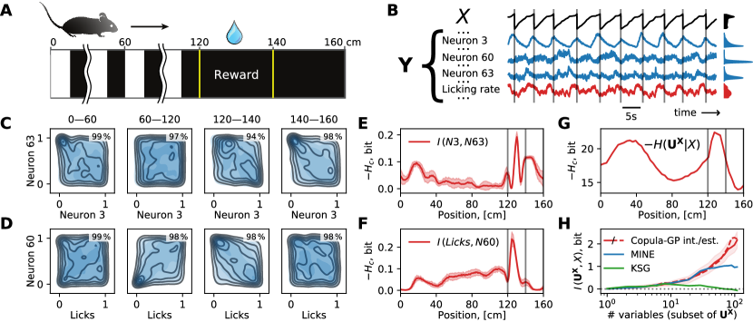
Figure 3: Applications of the Copula-GP framework to neuronal and behavioral data from the visual cortex. A Schematic of the experimental task [5, 45] in virtual reality (VR); B Example traces from ten example trials: $X$ is a position in VR, $\mathbf{Y}$ is a vector of neuronal recordings (blue) and behavioral variables (red); C-D Density plots for: the noise correlation (C) and the behavioral modulation (D) examples; E-G Conditional entropy for the bivariate examples (E-F) and the population-wide statistics (G); H Comparison of Copula-GP vs. non-parametric estimators on subsets of variables.

We investigate the dependencies observed in neuronal and behavioral data and showcase possible applications of the Copula-GP framework. We used two-photon calcium imaging data of neuronal population activity in the primary visual cortex of mice engaged in a visuospatial navigation task in virtual reality (data from Henschke et al. [45]). Briefly, the mice learned to run through a virtual corridor with vertical gratings on the walls (Fig. 3A, 0-120cm) until they reached a reward zone (Fig. 3A, 120-140cm), where they could get a reward by licking a reward spout. We condition our Copula-GP model on the position in the virtual environment $X$ and studied the joint distribution of the behavioral ($\tilde{Y}_{1}\ldots\tilde{Y}_{5}$) and neuronal ($\tilde{Y}_{6}\ldots\tilde{Y}_{109}$) variables ($\mathrm{dim}\mathbf{Y}$=109). Figure 3B shows a part of the dataset (trials 25-35 out of 130). The traces here demonstrate changes in the position $X$ of the mouse as well as the activity of 3 selected neurons and the licking rate. These variables have different patterns of activity depending on $X$ and different signal-to-noise ratios. Both differences are reflected in marginal statistics, which are shown on the right with the density plots of equal area.

Constructing interpretable bivariate models

We first studied bivariate relationships between neurons. In order to do this, we transformed the raw signals (shown in Fig. 3B) with a probability integral transform $\mathbf{U}=\mathbf{F}(\mathbf{Y})$. We observed strong non-trivial changes in the dependence structure $c(\mathbf{U}|X)$ subject to the position in the virtual reality $X$ and related visual information (Fig. 3C). Such stimulus-related changes in the joint variability of two neuronal signals are commonly described as noise correlations. The Copula-GP model provides a more detailed description of the joint probability that goes beyond linear correlation analysis. In this example, the dependence structure is best characterized by a combination of Gaussian and Clayton copula (rotated by 90^∘). The density plots Fig. 3C demonstrate the match between the true density (outlines) and the copula model density (blue shades) for each part of the task. We measure the accuracy of the density estimation with the proportion of variance explained $R^{2}$, which shows how much of the variance of the variable $Y_{2}$ can be predicted given the variable $Y_{1}$ (see Eq.(1) in Supplemental Material). The average $\overline{R^{2}}$ for all $Y_{1}$ is provided in the upper right corner of the density plots.

Next, we show that our model can be applied not only to the neuronal data, but also to any of the behavioral variables. Fig. 3D shows the dependence structure between one of the neurons and the licking rate. The best selected mixture model here is Frank + Clayton 0^∘ + Gumbel 270^∘, which again provides an accurate estimate of the conditional dependence between the variables. Therefore, Figs. 3C-D demonstrate that our Copula-GP model provides both an accurate fit for the probability distribution and an interpretable visualization of the dependence structure.

Figs. 3E-F show the absolute value of the conditional entropy $|H(\mathbf{U}^{X}|X)|$, which is equivalent to the mutual information between two variables $I(U_{1}^{X},U_{2}^{X})$. For both examples, the $\mathrm{MI}$ peaks in the reward zone. The bivariate Copula-GP models were agnostic of the reward mechanism in this task, yet they revealed the position of the reward zone as an anomaly in the mutual information.

Measuring information content in a large neuronal population

Finally, we constructed a C-vine describing the distribution between all neuronal and behavioral variables ($\mathrm{dim}\mathbf{U}^{X}=109$) and measured the conditional entropy $H(\mathbf{U}^{X}|X)$ for all variables in the dataset $\{U^{X}_{1}...U^{X}_{109}\}$. The conditional entropy in Fig. 3G peaks in the reward zone (similarly to Figs. 3E-F) and also at the beginning of the trial. Now the model is informed on the velocity of the animal and the reward events, so the first peak can be attributed to the acceleration of the mouse at the start of a new trial [46, 6].

While constructing the C-vine, we ordered the variables according to their pairwise rank correlations (see Sec. 2.3). We considered subsets of the first $N$ variables and measured the $\mathrm{MI}$ with the position for each subset. We compared the performance of our Copula-GP method on these subsets of $\mathbf{U^{X}}$ vs. KSG and MINE. Fig. 3H shows that all 3 methods provide similar results on subsets of up to 10 variables, yet in higher dimensions both MINE and KSG show smaller $I(X,\{U_{i<N}^{X}\})$ compared to our Copula-GP method, which agrees with the results obtained on the synthetic data (Fig. 2). The true values of $I(X,\{U_{i<N}^{X}\})$ are unknown, yet we expect the integrated Copula-GP (solid line) to underestimate the true value due to parametric model mismatch. The Copula-GP "estimated" (dashed line) almost perfectly matches the "integrated" result, which suggests that the model was able to accurately approximate both $p(\mathbf{U}^{X}|X)$ and $p(\mathbf{U}^{X})$, and, as a result, $I(X,\{U_{i<N}^{X}\})$. These results demonstrate superior performance of our Copula-GP model on high-dimensional neuronal data.

5 Discussion

We have developed a Copula-GP framework for modeling conditional multivariate joint distributions. The method is based on linear mixtures of parametric copulas, which provide flexibility for estimating complex dependencies. We approximate conditional dependencies of the model parameters with Gaussian Processes which allow us to implement a Bayesian model selection procedure. The selected models combine the accuracy in density estimation with the interpretability of parametric copula models. Despite the limitations of the parametric models, our framework demonstrated good results in mutual information estimation on the synthetically generated data, performing similarly to the state-of-the-art non-parametric information estimators. The framework is also well suited for describing neuronal and behavioral data. The possible applications include, but are not limited to, studying noise correlations, behavioral modulation and the neuronal population statistics. We demonstrated that the model scales well at least up to 109 variables, while theoretically, the parameter inference scales as $\mathcal{O}(n\cdot m^{2})$, where $n$ is a number of samples and $m$ is the (effective) number of variables (see Suppl. Mat.). In summary, we demonstrated that the Copula-GP approach can make stochastic relationships explicit and generate accurate and interpretable models of dependencies between neuronal responses, sensory stimuli, and behavior. Future work will focus on implementing model selection for the vine structure and improving the scalability of the $\mathrm{MI}$ estimation algorithm.

Broader Impact

We envision a wide range of impacts resulting from the use of the Copula-GP framework in computational neuroscience as well as in machine learning research, information technology and economics.

In computational neuroscience, this approach has the potential to reveal high dimensional context-dependent relationships between neuronal activity and behavioral variables. Therefore, our model can provide novel insights into the principles of neural circuit-level computation, both under physiological conditions, and during the aberrant network function observed in many neuropsychiatric disorders [47, 48, 49]. Furthermore, understanding context-dependent processing in the brain might suggest ways to mimic the same principles in artificial neural networks.

The proposed framework also has some potentially far reaching applications, not only in computational neuroscience but also in information technology and economics. Current problems of information flow in computer networks as well as high-speed trading in micro- and macro-markets can be phrased as non-stationary relationship problems that require proper stochastic representations, which, in turn, can benefit economic success. On the other hand, there is a possible risk of a one-sided adoption of the method by malicious actors benefiting from market manipulation, which may give them unfair advantage and thus reduce the market transparency and cause economic damage.

We encourage the researchers adapting our method to understand the limitations of the use of parametric copula models. The choice of the bivariate copula models and the vine structures introduces our beliefs about the particular conditional dependency or independency into the model. The misuse of parametric copula models has once had a negative impact on the insurance industry in the past [50]. Thus, these limitations must be taken into consideration when designing new applications in the future.

One potential negative societal impact related to the use of our framework may include a relatively large energy footprint from training the models on graphics processing units (GPUs). The models used for creating figures in this paper took about 2 weeks of computational time on 8 GPUs. The mitigation strategy should be focused on careful planning of the simulations, creating checkpoints and backups to prevent data loss, reuse of the trained models and other practices that reduce the energy-consuming computation.

Supplemental Material for “Parametric Copula-GP model for analyzing multidimensional neuronal and behavioral relationships”

 

S1 Methods

S1.1 Goodness-of-fit

We measure the accuracy of the density estimation with the proportion of variance explained $R^{2}$. We compare the empirical conditional CDF $\mathrm{ecdf}(U_{2}|U_{1}=y)$ vs. estimated conditional CDF $\mathrm{ccdf}(U_{2}|U_{1}=y)$ and calculate:

$$R^{2}(y)=1-\sum_{U_{2}}\left(\frac{\mathrm{ecdf}(U_{2}|U_{1}=y)-\mathrm{ccdf}(U_{2}|U_{1}=y)}{\mathrm{ecdf}(U_{2}|U_{1}=y)-\overline{U_{2}}}\right)^{2},$$ (S1)

where $R^{2}(y)$ quantifies the portion of the total variance of $U_{2}$ that our copula model can explain given $U_{1}=y$, and $\overline{U_{2}}=\overline{F(Y_{2})}=0.5$. The sum was calculated for $U_{2}=0.05n,n=0\ldots 20$.

Next, we select all of the samples from a certain interval of the task ($X\in[X_{1},X_{2}]$) matching one of those shown in Figure 3 in the paper. We split these samples $U_{1}\in[0,1]$ into 20 equally sized bins: $\{I_{i}\}_{20}$. For each bin $I_{i}$, we calculate (S1). We evaluate $\mathrm{ccdf}(U_{2}|U_{1}=y_{i})\approx\mathrm{ccdf}(U_{2}|U_{1}\in I_{i})$ using a copula model from the center of mass of the considered interval of $X$: $X_{\mu}=\mathrm{mean}(X)$ for samples $X\in[X_{1},X_{2}]$. We use the average measure:

$$\overline{R^{2}}=\mathop{\mathbb{E}}_{p(U_{1}\in I_{i})}R^{2}\big{(}\mathrm{mean}(U_{1}\in I_{i})\big{)},$$ (S2)

to characterize the goodness of fit for a bivariate copula model. Since $U_{1}$ is uniformly distributed on $[0,1]$, the probabilities for each bin $p(U_{1}\in I_{i})$ are equal to $1/20$, and the resulting measure $\overline{R^{2}}$ is just an average $R^{2}$ from all bins. The results were largely insensitive to the number of bins (e.g. 20 vs. 100).

S1.2 Variational inference

Since our model has latent variables with GP priors and intractable posterior distribution, the direct maximum likelihood Type-II estimation is not possible and an approximate inference is needed. We used stochastic variational inference (SVI) with a single evidence lower bound hensman2015scalable:

$$\mathcal{L}_{\mathrm{ELBO}}=\sum_{i=1}^{N}\mathop{\mathbb{E}}_{q(f_{i})}\big{[}\log p(y_{i}|f_{i})\big{]}-\mathop{\mathrm{KL}}[q(\mathbf{u})||p(\mathbf{u})],$$ (S3)

implemented as VariationalELBO in GPyTorch gardner2018gpytorchS. Here $N$ is the number of data samples, $\mathbf{u}$ are the inducing points, $q(\mathbf{u})$ is the variational distribution and $q(\mathbf{f})=\int p(\mathbf{f}|\mathbf{u})q(\mathbf{u})d\mathbf{u}$.

Following the wilson2015kernelS approach (KISS-GP), we then constrain the inducing points to a regular grid, which applies a deterministic relationship between $\mathbf{f}$ and $\mathbf{u}$. As a result, we only need to infer the variational distribution $q(\mathbf{u})$, but not the positions of $\mathbf{u}$. The number of grid points is one of the model hyper-parameters: grid_size.

Equation S3 enables joint optimization of the GP hyper-parameters (constant mean $\mu$ and two kernel parameters: scale and bandwidth) and parameters of the variational distribution $\mathbf{q}$ (mean and covariance at the inducing points: $\mathbf{u}\sim\mathcal{N}(\mu_{u}\times\mathbf{1},\Sigma_{u})$ ) hensman2015scalable. We have empirically discovered by studying the convergence on synthetic data, that the best results are achieved when the learning rate for the GP hyper-parameters (base_lr) is much greater than the learning rate for the variational distribution parameters (var_lr, see Table S1).

Priors

For both the neuronal and the synthetic data, we use a standard normal prior $p(\mathbf{u})\sim\mathcal{N}(\mathbf{0},I)$ for a variational distribution. Note, that the parametrization for mixture models was chosen such that the aforementioned choice of the variational distribution prior with zero mean corresponds to a priori equal mixing coefficients $\phi_{j}=1/M$ for $j=1\ldots M$. In our experiments with the simulated and real neuronal data, we observed that the GP hyper-parameter optimisation problem often had 2 minima (which is a common situation, see Figure 5.5 on page 116 in williams2006gaussian). One of those corresponds to a short kernel lengthscale ($\lambda$) and low noise ($\min_{\mathbf{f}}\sigma^{2}$), which we interpret as overfitting. To prevent overfitting, we used $\lambda\sim\mathcal{N}(0.5,0.2)$ prior on RBF kernel lengthscale parameter that allows the optimizer to approach the minima from the region of higher $\lambda$, ending up in the minimum with a larger lengthscale.

Optimization

We use the Adam optimizer with two learning rates for GP hyper-parameters (base_lr) and variational distribution parameters (var_lr). We monitor the loss (averaged over 50 steps) and its changes in the last 50 steps: $\Delta$ loss = mean(loss[-100:-50]) - mean(loss[-50:]). If the change becomes smaller than check_waic, then we evaluate the model $\mathrm{WAIC}$ and check if it is lower than $-\mathrm{WAIC}_{tol}$. If it is higher, we consider that either the variables are independent, or the model does not match the data. Either way, this indicates that further optimisation is counterproductive. If the $\mathrm{WAIC}<-\mathrm{WAIC}_{tol}$, we proceed with the optimisation until the change of loss in 50 steps $\Delta loss$ becomes smaller than loss_tol (see Table S1).

Effective learning rates for different families

The coefficients in the GPLink functions for different copula families are also a part of model hyper-parameters. The choice of these coefficients affects the gradients of the log probability function. Since GPLink functions are nonlinear, they affect the gradients in various parameter ranges to a different extent. This results in variable convergence rates depending on the true copula parameters.

To address the problem of setting up these hyper-parameters, we have created the tests on synthetic data with different copula parameters. Using these tests, we manually adjusted these hyper-parameters such that the GP parameter inference converged in around 1000-2000 iterations for every copula family and parameter range. We have also multiplied the GP values corresponding to the mixture coefficients by $0.5$, to effectively slow down the learning of the mixture coefficients $\phi$ compared to the copula coefficients $\theta$, which also facilitates the convergence.

Hyper-parameter selection

The hyper-parameters of our model (Table S1) were manually tuned, often considering the trade off between model accuracy and evaluation time. A more systematic hyper-parameter search might yield improved results and better determine the limits of model accuracy.

Table S1: Hyper-parameters of the bivariate Copula-GP model

Hyper-parameter	Value	Description
base_lr	$10^{-2}$	Learning rate for GP parameters
var_lr	$10^{-3}$	Learning rate for variational distribution
grid_size	128	Number of inducing points for KISS-GP
waic_tol	0.005	Tolerance for $\mathrm{WAIC}$ estimation
loss_tol	$10^{-4}$	Loss tolerance that indicates the convergence
check_waic	0.005	Loss tolerance when we check $\mathrm{WAIC}$
$\ldots$ and GPLink parameters listed in Table 1.

S1.3 Bayesian model selection

In model selection, we are aiming to construct a model with the lowest possible $\mathrm{WAIC}$. Since our copula probability densities are continuous, their values can exceed 1 and the resulting $\mathrm{WAIC}$ is typically negative. Zero $\mathrm{WAIC}$ corresponds to the Independence model ($\mathrm{pdf}=1$ on the whole unit square). We also set up a tolerance ($\mathrm{WAIC}_{tol}=0.005$), and models with $\mathrm{WAIC}\in[-\mathrm{WAIC}_{tol},\mathrm{WAIC}_{tol}]$ are considered indistinguishable from the independence model.

Since the total number of combinations of 10 copula elements (Fig.1) is large, exhaustive search for the optimal model is not feasible. In our framework, we propose two model algorithms for constructing close-to-optimal copula mixtures: greedy and heuristic.

S1.4 Model selection algorithms

1

2 $M,M_{\text{old}}\leftarrow[~{}],[~{}]$;

3 $S_{\text{c}}\leftarrow[\mathtt{Independence},\mathtt{Gauss},\mathtt{Frank},4\times\mathtt{Clayton},4\times\mathtt{Gumbel}]$;

4

5 // 4$\times$ includes all rotations

// while every update of the model yields a new best

6 while $\mathrm{WAIC}(M)\leq\mathrm{WAIC}(M_{\text{old}})$ and $\mathtt{size}(S_{\text{c}})>0$ do

7       $M_{\text{old}}\leftarrow M$ ;

8       select $c$ from $S_{\text{c}}$ such that $\mathrm{WAIC}(\mathtt{prepend}(c,M))$ is minimal;

9       $M\leftarrow\mathtt{prepend}(c,M)$ ;

10       remove $c$ from $S_{\text{c}}$;

11      

12 end while

13$M_{\text{best}}\leftarrow\mathtt{reduce}(M_{\text{old}})$;

14

15return $M_{\text{best}}$;

Algorithm 1 Greedy algorithm for copula mixture selection

1

2

3 $G\leftarrow[\mathtt{Gauss}]$;

4 if $\mathrm{WAIC}(G)>-\mathtt{waic\_tol}$ then

5       return $[\mathtt{Independence}]$;

6      

7 end if

8$M_{Cl}\leftarrow[\mathtt{Independence},\mathtt{Gauss},4\times\mathtt{Clayton}]$;

9 $M_{Gu}\leftarrow[\mathtt{Independence},\mathtt{Gauss},4\times\mathtt{Gumbel}]$;

10 $M_{\text{best}},M_{\text{worst}}\leftarrow$ ($M_{Cl}$,$M_{Gu}$) sorted by $\mathrm{WAIC}$;

11

12if $\mathrm{WAIC}(G)<\mathrm{WAIC}(M_{\text{best}})$ then

13       return $G$;

14      

15 end if

16

17for $i\leftarrow 3\ldots\mathtt{size}(M_{\text{best}})$ do

18       $M\leftarrow M_{\text{best}}$ with $i$-th element replaced by $M_{\text{worst}}[i]$;

19       $M_{\text{best}}\leftarrow M$ if $\mathrm{WAIC}(M)<\mathrm{WAIC}(M_{\text{best}})$;

20      

21 end for

22

23$M_{\text{best}}\leftarrow\mathtt{reduce}(M_{\text{best}})$;

24 if $\mathtt{Gauss}\in M_{\text{best}}$ then

25       $M\leftarrow M_{\text{best}}$ with $\mathtt{Gauss}$ replaced by $\mathtt{Frank}$;

26       $M_{\text{best}}\leftarrow M$ if $\mathrm{WAIC}(M)<\mathrm{WAIC}(M_{\text{best}})$;

27      

28 end if

// $\mathtt{Gauss}$ often gets confused with pairs of e.g. $\mathtt{Clayton}\,0^{\circ}+\mathtt{Gumbel}\,0^{\circ}$

29

30if $\mathtt{size}(M_{\text{best}})>1$ then

31       for $i\leftarrow 1\ldots(\mathtt{size}(M_{\text{best}})-1)$ do

32             for $j\leftarrow(i+1)\ldots\mathtt{size}(M_{\text{best}})$ do

33                   $M\leftarrow M_{\text{best}}$ with $i$-th and $j$-th elements removed;

34                   $M\leftarrow\mathtt{prepend}(\mathtt{Gauss},M)$;

35                   if $\mathrm{WAIC}(M)<\mathrm{WAIC}(M_{\text{best}})$ then

36                         $M_{\text{best}}\leftarrow M$ ;

37                         break ;

38                        

39                   end if

40                  

41             end for

42            

43       end for

44      

45 end if

46

47$M_{\text{best}}\leftarrow\mathtt{reduce}(M_{\text{best}})$;

48

49return $M_{\text{best}}$;

50

Algorithm 2 Heuristic algorithm for copula mixture selection

The greedy algorithm (Algorithm 1) starts by comparing $\mathrm{WAIC}$ of all possible single-copula models (from Table 1, in all rotations) and selecting the model with the lowest $\mathrm{WAIC}$. After that, we add one more copula (from another family or in another rotation) to the first selected copula, and prepend the element that yields the lowest $\mathrm{WAIC}$ of the mixture. We repeat the process until the $\mathrm{WAIC}$ stops decreasing. After the best model is selected, we remove the inessential elements using the reduce(.) function. This function removes those elements which have an average concentration of $<10\%$ everywhere on $X\in[0,1]$. This step is added to improve the interpretability of the models and computation time for entropy estimation (at a small accuracy cost) and can, in principle, be omitted.

The greedy algorithm can be improved by adding model reduction after each attempt to add an element. In this case, the number of elements can increase and decrease multiple times during the model selection process, which also must be terminated if the algorithm returns to the previously observed solution. Even though it complicates the algorithm, it reduces the maximal execution time (observed on the real neuronal data) from $\sim$90 minutes down to $\sim$40 minutes.

The heuristic algorithm focuses on the tail dependencies (Algorithm 2). First, we try a single Gaussian copula. If variables are not independent, we next compare 2 combinations of 6 elements, which are organized as follows: an Independence copula together with a Gaussian copula and either 4 Clayton or 4 Gumbel copulas in all 4 rotations (0^∘, 90^∘, 180^∘, 270^∘). We select the combination with the lowest $\mathrm{WAIC}$. After that, we take the remaining Clayton/Gumbel copulas one by one and attempt to switch the copula type (Clayton to Gumbel or vise versa). If this switching decreases the $\mathrm{WAIC}$, we keep a better copula type for that rotation and proceed to the next element.

Here we make the assumption, that because Clayton and Gumbel copulas have most of the probability density concentrated in one corner of the unit square (the heavy tail), we can choose the best model for each of the 4 corners independently. When the best combination of Clayton/Gumbel copulas is selected, we can (optionally) reduce the model.

We have not yet used a Frank copula in a heuristic algorithm. We attempt to substitute the Gaussian copula with a Frank copula (if it is still a part of the reduced mixture, see lines 16-19 in Alg. 2). Sometimes, a Gaussian copula can be mistakenly modeled as a Clayton & Gumbel or two Gumbel copulas. So, as a final step (lines 20-31, Alg. 2), we select all pairwise combinations of the remaining elements, and attempt to substitute each of the pairs with a Gaussian copula, selecting the model with the lowest $\mathrm{WAIC}$. Despite a large number of steps in this algorithm, the selection process takes only up to 25 minutes (in case all elements in all rotations are required).

The procedure was designed after observing the model selection process on a variety of synthetic and real neuronal datasets.

S1.5 Vine copulas

Vine models provide a way to factorize the high-dimensional copula probability density into a hierarchical set of bivariate copulas aas2009pairS. There are many possible decompositions based on different assumptions about conditional independence of specific elements in a model, which can be classified using graphical models called regular vines bedford2001probability,bedford2002vines. A regular vine can be represented using a hierarchical set of trees, where each node corresponds to a conditional distribution function (e.g. $F(U_{2}|U_{1})$) and each edge corresponds to a bivariate copula (e.g. $c(U_{2},U_{3}|U_{1})$). The copula models from the lower trees are used to obtain new conditional distributions (new nodes) with additional conditional dependencies for the higher trees, e.g. a ccdf of a copula $c(U_{2},U_{3}|U_{1})$ and a marginal conditional distribution $F(U_{2}|U_{1})$ from the 1st tree provide a new conditional distribution $F(U_{3}|U_{1},U_{2})$ for a 2nd tree. Therefore, bivariate copula parameters are estimated sequentially, starting from the lowest tree and moving up the hierarchy. The total number of edges in all trees (= the number of bivariate copula models) for an $m$-dimensional regular vine equals $m(m-1)/2$.

The regular vines often assume that the conditional copulas $c(U_{i},U_{j}|\{U_{k}\})$ themselves are independent of their conditioning variables $\{U_{k}\}$, but depend on the them indirectly through the conditional distribution functions (nodes) acar2012beyond. This is known as the simplifying assumption for vine copulas haff2010simplified, which, if applicable, allows to escape the curse of dimensionality in high-dimensional copula construction.

In this study, we focus on the canonical vine or C-vine, which has a unique node in each tree, connected to all of the edges in that tree. For illustration, see, for example, Figure 2 in aas2009pair. The C-vine was shown to be a good choice for neuronal datasets onken2016nipsS, as they often include some proxy of neuronal population activity as an outstanding variable, strongly correlated with the rest. This variable provides a natural choice for the first conditioning variable in the lowest tree. In the neuronal datasets from henschke2020rewardS, this outstanding variable is the global fluorescence signal in the imaged field of view (global neuropil).

To construct a C-vine for describing the neuronal and behavioural data from henschke2020rewardS, we used a heuristic element ordering based on the sum of absolute values of Kendall’s $\tau$ of a given element with all of the other elements. It was shown by czado2012maximumS that this ordering facilitates C-vine modeling. For all of the animals and most of the recordings (14 out of 16), including the one used in Figure 3, the first variable after such ordering was the global neuropil activity. This again confirms, that a C-vine with the global neuropil activity as a first variable is an appropriate model for the dependencies in neuronal datasets.

S1.6 Algorithmic complexity

In this section, we discuss the algorithmic complexity of the parameter inference for a C-vine copula model.

The parameter inference for each of the bivariate Copula-GP models scales as $\mathcal{O}(n)$, where $n$ is the number of samples, since we use a scalable kernel interpolation KISS-GP wilson2015kernel. As we mentioned in Sec. S1.5, a full $m$-dimensional C-vine model requires $m(m-1)/2$ bivariate copulas, trained sequentially. As a result, the $\mathcal{O}(n)$ GP parameter inference has to be repeated $m(m-1)/2$ times, which yields $\mathcal{O}(n\cdot m^{2})$ complexity.

In practice, the computational cost (in terms of time) of the parameter inference for each bivariate model varies from tens of seconds to tens of minutes. The heuristic model selection is designed in such a way, that it discards independent variables in just around 20 seconds (line 3 in Alg. 2). As a result, most of the models are quickly skipped and further considered as Independence models, and their contribution to the total computational cost can be neglected. When the model is evaluated, the Independence components are also efficiently ‘skipped’ during sampling, as ppcf function is not called for them. The Independence models also add zero to C-vine log probability, so they are also ‘skipped’ during log probability calculation. They also reduce the total memory storage, as no GP parameters, which predominate the memory requirements, are stored for these models.

In a conditional C-vine trained on a real neuronal dataset with 109 variables, 5253 out of 5886 (89%) bivariate models were Independence, which leaves only 633 non-Independence models.

In practice, this means that the algorithmic complexity of the model is much better than the naïve theoretical prediction $\mathcal{O}(n\cdot m^{2})$, based on the structure of the graphical model. Suppose that the actual number of the non-Independence models $N_{nI}$ in a vine model is much smaller than $m(m-1)/2$ and can be characterized by an effective number of dimensions $m_{eff}\sim\sqrt{N_{nI}}$. In this case, instead of the $\mathcal{O}(m^{2})$ scaling with the number of variables, the complexity highly depends on the sparsity of the dependencies in the graphical model and scales with as $\mathcal{O}(n\cdot N_{nI})\sim\mathcal{O}(n\cdot m_{eff}^{2})$.

Therefore, the our method is especially efficient on the datasets with a low effective dimensionality $m_{eff}$, such as the neuronal data. The number of variables $m$ itself has little effect on the computational cost and memory storage.

S2 More validation on synthetic data

Computing infrastructure

We developed our framework and ran the majority of our experiments (described both in the paper and Supplemental Material) on an Ubuntu 18.04 LTS machine with 2 x Intel(R) Xeon(R) Gold 6142 CPU @ 2.60GHz and 1x GeForce RTX 2080 + 1 x GeForce RTX 2080 Ti GPUs. For training C-vine models, we used another Scientific Linux 7.6 machine with 1 x Intel(R) Xeon(R) Silver 4114 CPU @ 2.20GHz and 8 x GeForce RTX 2080 Ti GPUs.

Code availability

Code will be made available on GitHub upon paper acceptance.

S2.1 Model selection for bivariate copulas

Synthetic data

We generate artificial data by sampling from a copula mixture, parametrized in two different ways:

1. mixing concentrations of all copulas were constant and equal to $1/N$ ($N$ = number of copulas), but copula parameters $\theta$ were parametrized by the phase-shifted sinus functions:

   $$\theta_{i}=A_{i}\sin\left(\pi m\frac{i}{N}+2\pi x\right)+B_{i},\qquad x\in[0,1]$$ (S4)

   where $i$ is the index of the copula in a mixture, $m=1$. For Clayton and Gumbel copulas, the absolute value of the sinus was used. The amplitudes $A_{i}$ were chosen to cover most of the range of parameters, except for extremely low or high $\theta$s for which all copula families become indistinguishable (from independence or deterministic dependence, respectively).

2. copula parameters $\theta$ were constant, but mixing concentrations $\phi$ were parametrized by the phase-shifted sinus functions (same as Eq. S4, with $A_{i}=B_{i}=1/N$ and $m=2$). Such parametrization ensures that the sum of all mixing concentrations remains equal to one ($\sum_{i=1}^{N}\phi=1$). Yet, each $\phi$ turns to zero somewhere along this trajectory, allowing us to discriminate the models and infer the correct mixture.

Identifiability tests

We tested the ability of the model selection algorithms to select the correct mixture of copula models, the same as the one from which the data was generated. We generated 5000 samples with equally spaced unique inputs on [0,1].

Both model selection algorithms were able to correctly select all of the 1-component and most of the 2-component models on simulated data. For simulated data with larger numbers of components (or 2 very similar components), the $\mathrm{WAIC}$ of the selected model was either lower (which is possible given a limited number of samples) or close to the $\mathrm{WAIC}$ of the correct parametric model. In other words, the difference between the $\mathrm{WAIC}$ of the correct model and of the best selected model never exceeded the $\mathrm{WAIC}_{test\_tol}=0.05$, which we set up as a criteria for passing the test: $\Delta\mathrm{WAIC}<\mathrm{WAIC}_{test\_tol}$. Since all the tests were passed successfully, we conclude that both algorithms are capable of finding optimal or close-to-optimal solutions for copula mixtures.

A more detailed report on the model identifiability tests

Tables S2-LABEL:tab:search3T below illustrate the search for the best model. The copula model names in these tables are shortened to the first two letters, e.g. Gumbel becomes ‘Gu’, Frank becomes ‘Fr’. The information in these Tables provides some intuition on the model selection process and the range of $\mathrm{WAIC}$s for the correct or incorrect models. The final selected models are shown in bold.

Table S2 demonstrates that both greedy and heuristic algorithms can identify the correct single copula model. Some key intermediate models ($M$ in Alg. 1-2) with their $\mathrm{WAIC}$s are listed in the table, along with the total duration of simulations (T, in minutes) on RTX 2080Ti  for both algorithms.

Table LABEL:tab:search2M shows the identification of the mixtures with 2 components, where the copula parameters $\theta$ were constant (independent of $X$) and mixing concentrations $\phi$ were parameterized by the phase-shifted sinus functions (Eq. S4). All of these models were correctly identified with both algorithms. The mixtures with 2 components, where the copula parameters $\theta$ varied harmonically (as in Eq. S4) but the mixing concentrations $\phi$ were constant, were harder to identify. Table LABEL:tab:search2T shows that a few times, each of the algorithms selected a model that was better than the true model ($\mathrm{WAIC}_{best}-\mathrm{WAIC}_{true}<0$). The greedy algorithm made one mistake, yet the model it selected was very close to optimal. Such misidentification happens due to the limited number of samples in a given synthetic dataset.

Tables LABEL:tab:search3M-LABEL:tab:search3T show the model selection for 3 component models. Again, as in Tables LABEL:tab:search2M-LABEL:tab:search2T, either $\theta$ or $\phi$ was constant. Here, the model selection algorithms could rarely identify the correct model (due to overcompleteness of the mixture models), but always selected the one that was very close to optimal: $\mathrm{WAIC}_{best}-\mathrm{WAIC}_{true}\ll\mathrm{WAIC}_{test\_tol}$.

Note, that $\mathrm{WAIC}_{test\_tol}$ is different from waic_tol. We have set waic_tol for comparison against Independent model to such a small value (10x smaller than $\mathrm{WAIC}_{test\_tol}$) because we want to avoid making false assumptions about conditional independences in the model. Also note, that the $\mathrm{WAIC}$ of the true model depends on the particular synthetic dataset generated in each test. Therefore, the final $\mathrm{WAIC}$ in the left and in the right columns of Tables S2-LABEL:tab:search3T can be slightly different (yet, right within $\mathrm{WAIC}_{test\_tol}$).

S2.2 Accuracy of entropy estimation

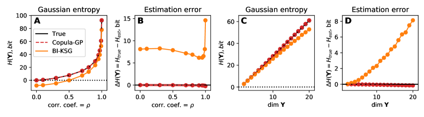
Figure S4: Accuracy of the entropy estimation for multivariate Gaussian distributions. A Entropy of the 20-dimensional multivariate Gaussian distribution for different correlation coefficients $\rho$. B Estimation error for the entropy shown in A. C Entropy of the multivariate Gaussian distributions with $\rho=0.99$ and varying dimensionality. D Estimation error for the entropy shown in C.

In this section, we consider a fixed copula mixture model with known parameters $\theta$ and test the reliability of the entropy estimation with Monte Carlo (MC) integration. We test the accuracy of the entropy estimation on a multivariate Gaussian distribution, with $\mathrm{cov}(Y_{i},Y_{j})=\rho+(1-\rho)\,\delta_{ij}$, where $\delta_{ij}$ is Kronecker’s delta and $\rho\in~{}[0,0.999]$. Given a known Gaussian copula, we estimate the entropy with MC integration and compare it to the analytically calculated true value. We set up a tolerance to $\Delta H=0.01(\mathrm{dim}\mathbf{Y})$. As a result, for every correlation $\rho$ (Fig. S4A-B) and every number of dimensions $\mathrm{dim}\mathbf{Y}$ (Fig. S4C-D), the Copula-GP provides an accurate result, within the error margin. In Figure S4, BI-KSG estimates gao2016demystifyingS obtained on the dataset with 10k samples are shown for comparison. This experiment 1) validates the MC integration; 2) validates the numerical stability of the probability density function of the Gaussian copula up to a specified maximal $\rho=0.999$ (for $\rho>0.999$ the model is indistinguishable from the deterministic dependence $U_{1}=U_{2}$).

S3 Model parameters for the bivariate neuronal and behavioural examples

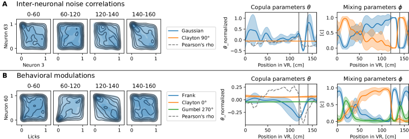
Figure S5: Parameters of the copula mixture models. From left to right: copula probability densities (same as Fig.3C-D); a list of selected copula elements; copula parameters $\theta$; mixing concentrations $\phi$. These plots are provided for: A the noise correlation example; B the behavioral modulation example.

In this section, we provide visualisations for the parameters of the bivariate copula models from Figure 3C-F and discuss the interpretability of these models.

Figure S5 shows the probability density of the joint distribution of two variables and the parameters of a corresponding Copula-GP mixture model. The plots on the left repeat Fig.3C-D and represent the true density (outlines) and the copula model density (blue shades) for each part of the task.

In the noise correlation example (Fig. S5A), we observe the tail dependencies between the variables (i.e. concentration of the probability density in a corner of the unit square) around [0-60] cm and [140-160] cm of the virtual corridor. There is only one element with a tail dependency in this mixture: Clayton 90^∘ copula. On the right-most plot in Fig. S5A, we see the mixing concentration for the elements of the mixture model. The concentration of Clayton 90^∘ copula (orange line) is close to 100% around 20 cm and 150 cm, which agrees with our observations from the density plots.

The confidence intervals ($\pm 2\sigma$) for the parameters approximated with Gaussian processes are shown with shaded areas in parameter plots. These intervals provide a measure of uncertainty in model parameters. For instance, when the concentration of the Gaussian copula in the mixture is close to 0% ($X$ around 20 cm and 150 cm), the confidence intervals for the Gaussian copula parameter ($\theta$, blue shade) in Fig. S5A become very wide (from almost 0 to 1). Since this copula element is not affecting the mixture for those values of $X$, its $\theta$ parameter has no effect on the mixture model log probability. Therefore, this parameter is not constrained to any certain value. In a similar manner, we see that the variables are almost independent between 60 and 120 cm (see density plots on the left in Fig. S5). Both copula elements can describe this independence. As a result, the mixing concentrations for both elements have high uncertainty in that interval of $X$. Yet, Gaussian copula with a slightly positive correlation is still a bit more likely to describe the data in that interval.

The copula parameter plot in Fig. S5A also shows Pearson’s $\rho$, which does not change much in this example and remains close to zero. This illustrates, that the traditional linear noise correlation analysis would ignore (or downplay) this pair of neurons as the ones with no dependence. This happens because the Pearson’s $\rho$ only captures the linear correlation and ignores the tail dependencies, whereas our model provides a more detailed description of the joint bivariate distribution.

In the behavioural modulation example (Fig. S5B), we observe more complicated tail dependencies in the density plots. The best selected model supports this observation and provides a mixture model with 3 components, 2 of which have various tail dependencies. The Clayton 0^∘ copula (orange) describes the lower tail dependence observed in the second part of the virtual corridor with gratings (around [60-120] cm, see Fig. 3A for task structure). This dependence can be verbally interpreted as follows: when there is no licking, the Neuron 60 is certainly silent; but when the animal is licking, the activity of Neuron 60 is slightly positively correlated with the licking rate.

These examples illustrate, that by analysing the copula parameters and the mixing concentrations of the Copula-GP mixture model, one can interpret the changes in the bivariate dependence structure. Just like traditional tuning curves characterize the response of a single neuron, our mixture model characterizes the ‘tuning’ of the dependence structure between pairs of variables to a given stimulus or context. Knowing the qualitative properties of the copula elements that constitute a copula mixture, one can focus on the dominant element of the copula mixture for every given conditioning variable $X$ and describe the shape of the dependence.

unsrtnat references_Suppl_1

Table S2: The model selection histories for 1-element mixtures

True	Greedy			Heuristic
Model	Search attempts	WAIC	T	Search attempts	WAIC	T
Ga	Ga	-0.1619	25 m	Ga	-0.1513	3 m
	GaFr	-0.1610		InGaGu180Gu270Gu0Gu90	-0.1499
	Ga	-0.1619		InGaCl0Cl90Cl180Cl270	-0.1498
				Ga	-0.1513
Fr	Fr	-0.1389	57 m	Ga	-0.1400	3 m
	FrCl90	-0.1395		InGaGu180Gu270Gu0Gu90	-0.1391
	FrCl90Gu270	-0.1396		InGaCl0Cl90Cl180Cl270	-0.1391
	FrCl90Gu270Gu90	-0.1396		Fr	-0.1509
	Fr	-0.1389
Cl0	Cl0	-0.5225	37 m	Ga	-0.3825	5 m
	Cl0Gu0	-0.5226		InGaGu180Gu270Gu0Gu90	-0.4943
	Cl0Gu0Cl180	-0.5225		InGaCl0Cl90Cl180Cl270	-0.5303
	Cl0	-0.5224		Cl0	-0.5311
Gu0	Gu0	-0.6267	43 m	Ga	-0.5555	7 m
	Gu0Cl180	-0.6268		InGaGu180Gu270Gu0Gu90	-0.5988
	Gu0Cl180Gu180	-0.6267		InGaCl0Cl90Cl180Cl270	-0.5946
	Gu0	-0.6230		GaGu0	-0.6040
				Gu0	-0.6050
Cl90	Cl90	-0.5389	22 m	Ga	-0.3922	5 m
	Cl90Cl270	-0.5389		InGaGu180Gu270Gu0Gu90	-0.5047
	Cl90	-0.5389		InGaCl0Cl90Cl180Cl270	-0.5409
				Cl90	-0.5410
Gu90	Gu90	-0.6137	55 m	Ga	-0.5501	7 m
	Gu90Gu270	-0.6144		InGaGu180Gu270Gu0Gu90	-0.5893
	Gu90Gu270Cl270	-0.6145		InGaCl0Cl90Cl180Cl270	-0.5831
	Gu90Gu270Cl270Cl90	-0.6144		GaGu90	-0.5887
	Gu90	-0.6137		Gu90	-0.5950
Cl180	Cl180	-0.5566	36 m	Ga	-0.3932	7 m
	Cl180Cl0	-0.5582		InGaGu180Gu270Gu0Gu90	-0.4956
	Cl180Cl0In	-0.5582		InGaCl0Cl90Cl180Cl270	-0.5493
	Cl180	-0.5565		Cl180	-0.5489
Gu180	Gu180	-0.6131	43 m	Ga	-0.5553	6 m
	Gu180Cl0	-0.6164		InGaGu180Gu270Gu0Gu90	-0.6091
	Gu180Cl0Fr	-0.6163		InGaCl0Cl90Cl180Cl270	-0.6045
	Gu180	-0.6131		Gu180	-0.6154
Cl270	Cl270	-0.5434	23 m	Ga	-0.3909	5 m
	Cl270Gu270	-0.5433		InGaGu180Gu270Gu0Gu90	-0.5094
	Cl270	-0.5434		InGaCl0Cl90Cl180Cl270	-0.5535
				Cl270	-0.5548
Gu270	Gu270	-0.5928	51 m	Ga	-0.5763	6 m
	Gu270Cl90	-0.5934		InGaGu180Gu270Gu0Gu90	-0.6277
	Gu270Cl90In	-0.5935		InGaCl0Cl90Cl180Cl270	-0.6179
	Gu270Cl90InCl180	-0.5931		Gu270	-0.6300
	Gu270	-0.5928

Table S3: The model selection histories for 2-element mixtures with constant $\theta$ and variable $\phi$

True	Greedy			Heuristic
Model	Search attempts	WAIC	T	Search attempts	WAIC	T
Gu90	Ga	-0.1877	101 m	Ga	-0.1922	11 m
Ga	GaGu90	-0.2855		InGaGu180Gu270Gu0Gu90	-0.3070
	GaGu90Cl270	-0.2855		InGaCl0Cl90Cl180Cl270	-0.2996
	GaGu90Cl270Fr	-0.2856		GaCl0Gu0Gu90	-0.3082
	GaGu90Cl270FrGu270	-0.2856		GaCl0Cl180Gu90	-0.3076
	GaGu90Cl270FrGu270Cl90	-0.2856		GaGu90	-0.3091
	Gu90Ga	-0.2854
Ga	Fr	-0.1635	87 m	Ga	-0.1600	5 m
Cl270	FrCl270	-0.2707		InGaGu180Gu270Gu0Gu90	-0.2687
	FrCl270Ga	-0.2747		InGaCl0Cl90Cl180Cl270	-0.2835
	FrCl270GaGu180	-0.2782		GaCl270	-0.2845
	FrCl270GaGu180Cl90	-0.2781
	GaCl270	-0.2821
Gu180	Gu180	-0.1681	99 m	Ga	-0.1534	8 m
Fr	Gu180Fr	-0.2099		InGaGu180Gu270Gu0Gu90	-0.1993
	Gu180FrCl180	-0.2101		InGaCl0Cl90Cl180Cl270	-0.1977
	Gu180FrCl180Cl90	-0.2105		InGaGu180	-0.2074
	Gu180FrCl180Cl90In	-0.2106		FrGu180	-0.2104
	Gu180FrCl180Cl90InGu270	-0.2099
	FrGu180	-0.2099
Cl0	Fr	-0.1587	92 m	Ga	-0.1652	5 m
Cl90	FrCl0	-0.2600		InGaGu180Gu270Gu0Gu90	-0.3142
	FrCl0Cl90	-0.3173		InGaCl0Cl90Cl180Cl270	-0.3430
	FrCl0Cl90Gu270	-0.3176		Cl0Cl90	-0.3448
	FrCl0Cl90Gu270In	-0.3176
	FrCl0Cl90Gu270InCl270	-0.3175
	Cl90Cl0	-0.3190
Cl180	Fr	-0.2204	103 m	Ga	-0.1965	7 m
Gu270	FrCl180	-0.3488		InGaGu180Gu270Gu0Gu90	-0.3591
	FrCl180Gu270	-0.3874		InGaCl0Cl90Cl180Cl270	-0.3688
	FrCl180Gu270Cl90	-0.3877		GaGu270Cl180	-0.3771
	FrCl180Gu270Cl90Ga	-0.3878		Gu270Cl180	-0.3772
	FrCl180Gu270Cl90GaGu90	-0.3878
	Gu270Cl180	-0.3888

Table S4: The model selection histories for 2-element mixtures with constant $\phi$ and variable $\theta$

True	Greedy			Heuristic
Model	Search attempts	WAIC	T	Search attempts	WAIC	T
Gu90	Gu90	-0.1419	60 m	Ga	-0.1538	10 m
Ga	Gu90Fr	-0.2022		InGaGu180Gu270Gu0Gu90	-0.2320
	Gu90FrCl270	-0.2024		InGaCl0Cl90Cl180Cl270	-0.2218
	Gu90FrCl270Ga	-0.2024		GaCl90Gu0Gu90	-0.2321
	FrGu90	-0.2021		GaGu90	-0.2326
	$\mathrm{WAIC}_{best}-\mathrm{WAIC}_{true}$:	-0.0013
Ga	Gu90	-0.1495	56 m	Ga	-0.1062	7 m
Cl270	Gu90Fr	-0.1894		InGaGu180Gu270Gu0Gu90	-0.1747
	Gu90FrCl270	-0.1915		InGaCl0Cl90Cl180Cl270	-0.1783
	Gu90FrCl270In	-0.1902		GaGu0Cl270	-0.1812
	Cl270FrGu90	-0.1915		GaCl270	-0.1801
	$\mathrm{WAIC}_{best}-\mathrm{WAIC}_{true}$:	0.0032
Gu180	Gu180	-0.1600	58 m	Ga	-0.1331	8 m
Fr	Gu180Fr	-0.2191		InGaGu180Gu270Gu0Gu90	-0.1944
	Gu180FrCl270	-0.2195		InGaCl0Cl90Cl180Cl270	-0.1936
	Gu180FrCl270Cl0	-0.2190		GaGu180Cl90Gu0Gu90	-0.1945
	FrGu180	-0.2190		GaGu180	-0.1992
				$\mathrm{WAIC}_{best}-\mathrm{WAIC}_{true}$:	-0.0094
Cl0	Gu180	-0.0253	62 m	Ga	-0.0079	5 m
Cl90	Gu180Cl90	-0.2383		InGaGu180Gu270Gu0Gu90	-0.1904
	Gu180Cl90Cl0	-0.2506		InGaCl0Cl90Cl180Cl270	-0.2330
	Gu180Cl90Cl0In	-0.2509		Cl0Cl90	-0.2361
	Gu180Cl90Cl0InFr	-0.2508
	Cl0Cl90	-0.2586
Cl180	Gu270	-0.0242	69 m	Ga	-0.0083	6 m
Gu270	Gu270Cl180	-0.2499		InGaGu180Gu270Gu0Gu90	-0.2277
	Gu270Cl180Gu180	-0.2517		InGaCl0Cl90Cl180Cl270	-0.2535
	Gu270Cl180Gu180In	-0.2518		GaCl90Cl180	-0.2549
	Gu270Cl180Gu180InCl0	-0.2518
	Gu270Cl180Gu180InCl0Fr	-0.2518
	Cl180Gu270	-0.2500
				$\mathrm{WAIC}_{best}-\mathrm{WAIC}_{true}$:	-0.0098

Table S5: The model selection histories for 3-element mixtures with constant $\theta$ and variable $\phi$

True	Greedy			Heuristic
Model	Search attempts	WAIC	T	Search attempts	WAIC	T
Ga	Gu0	-0.1399	44 m	Ga	-0.1252	6 m
Cl90	Gu0Cl90	-0.2494		InGaGu180Gu270Gu0Gu90	-0.2481
Gu0	Gu0Cl90Cl0	-0.2519		InGaCl0Cl90Cl180Cl270	-0.2565
	Gu0Cl90Cl0Fr	-0.2518		GaCl90Cl180	-0.2564
	Cl90Gu0	-0.2494
	$\mathrm{WAIC}_{best}-\mathrm{WAIC}_{true}$:	-0.0036		$\mathrm{WAIC}_{best}-\mathrm{WAIC}_{true}$:	0.0014
Fr	Fr	-0.0591	77 m	Ga	-0.0489	6 m
Cl90	FrCl90	-0.1460		InGaGu180Gu270Gu0Gu90	-0.1573
Gu0	FrCl90Gu0	-0.1730		InGaCl0Cl90Cl180Cl270	-0.1578
	FrCl90Gu0Cl180	-0.1736		GaCl90Cl180	-0.1621
	FrCl90Gu0Cl180In	-0.1734
	Gu0Cl90Fr	-0.1731
				$\mathrm{WAIC}_{best}-\mathrm{WAIC}_{true}$:	0.0059
Fr	Fr	-0.0741	87 m	Ga	-0.0618	9 m
Cl180	FrCl180	-0.1513		InGaGu180Gu270Gu0Gu90	-0.1567
Gu270	FrCl180Gu270	-0.1707		InGaCl0Cl90Cl180Cl270	-0.1670
	FrCl180Gu270Cl90	-0.1708		InGaGu270Cl180Cl270	-0.1680
	FrCl180Gu270Cl90Gu180	-0.1711		InGaGu270Cl180Gu90	-0.1695
	FrCl180Gu270Cl90Gu180Cl0	-0.1710		InGu270Cl180	-0.1735
	Gu270Cl180Fr	-0.1703
				$\mathrm{WAIC}_{best}-\mathrm{WAIC}_{true}$:	-0.0011
Gu0	Gu0	-0.1695	47 m	Ga	-0.1477	11 m
Gu180	Gu0Cl90	-0.3040		InGaGu180Gu270Gu0Gu90	-0.2986
Cl90	Gu0Cl90Gu180	-0.3234		InGaCl0Cl90Cl180Cl270	-0.3033
	Gu0Cl90Gu180Cl180	-0.3233		GaGu180Cl90Cl180	-0.3054
	Gu180Cl90Gu0	-0.3234		GaGu180Cl90Gu0	-0.3111
				Gu180Cl90Gu0	-0.3113

Table S6: The model selection histories for 3-element mixtures with constant $\phi$ and variable $\theta$

True	Greedy			Heuristic
Model	Search attempts	WAIC	T	Search attempts	WAIC	T
Ga	Fr	-0.0177	66 m	Ga	-0.0142	13 m
Cl90	FrGu270	-0.1284		InGaGu180Gu270Gu0Gu90	-0.1291
Gu0	FrGu270Gu0	-0.1407		InGaCl0Cl90Cl180Cl270	-0.1289
	FrGu270Gu0Cl0	-0.1423		InCl0Gu270Gu0	-0.1317
	FrGu270Gu0Cl0Cl180	-0.1435		InCl0Cl90Gu0	-0.1346
	FrGu270Gu0Cl0Cl180In	-0.1432		InCl0Cl90Cl180	-0.1301
	Gu0Gu270	-0.1451		GaCl90Cl180	-0.1313
	$\mathrm{WAIC}_{best}-\mathrm{WAIC}_{true}$:	0.0132		$\mathrm{WAIC}_{best}-\mathrm{WAIC}_{true}$:	0.0068
Fr	Fr	-0.0265	71 m	Ga	-0.0192	9 m
Cl90	FrGu270	-0.1290		InGaGu180Gu270Gu0Gu90	-0.1411
Gu0	FrGu270Gu0	-0.1445		InGaCl0Cl90Cl180Cl270	-0.1429
	FrGu270Gu0Cl180	-0.1450		InGaGu180Cl90Cl180	-0.1474
	FrGu270Gu0Cl180Cl0	-0.1466		InGaGu180Cl90Gu0	-0.1472
	FrGu270Gu0Cl180Cl0In	-0.1468		InCl90Gu0	-0.1477
	Gu0Gu270	-0.1451
	$\mathrm{WAIC}_{best}-\mathrm{WAIC}_{true}$:	0.0109		$\mathrm{WAIC}_{best}-\mathrm{WAIC}_{true}$:	0.0010
Fr	Fr	-0.0129	61 m	Ga	-0.0185	6 m
Cl180	FrGu270	-0.1105		InGaGu180Gu270Gu0Gu90	-0.1309
Gu270	FrGu270Gu0	-0.1237		InGaCl0Cl90Cl180Cl270	-0.1326
	FrGu270Gu0Cl180	-0.1254		InGu270Cl180	-0.1393
	FrGu270Gu0Cl180Gu180	-0.1248		InGu270Gu0	-0.1334
	Gu0Gu270Fr	-0.1234		InGu270Gu0	-0.1326
	$\mathrm{WAIC}_{best}-\mathrm{WAIC}_{true}$:	0.0094		$\mathrm{WAIC}_{best}-\mathrm{WAIC}_{true}$:	0.0088
Gu0	Gu0	-0.0756	55 m	Ga	-0.0454	7 m
Gu180	Gu0Cl90	-0.2380		InGaGu180Gu270Gu0Gu90	-0.2476
Cl90	Gu0Cl90Cl0	-0.2556		InGaCl0Cl90Cl180Cl270	-0.2459
	Gu0Cl90Cl0Ga	-0.2591		GaCl0Gu270Gu0	-0.2493
	Gu0Cl90Cl0GaCl270	-0.2590		GaCl0Cl90Gu0	-0.2559
	Cl0Cl90Gu0	-0.2555		Cl0Cl90Gu0	-0.2538
	$\mathrm{WAIC}_{best}-\mathrm{WAIC}_{true}$:	0.0026		$\mathrm{WAIC}_{best}-\mathrm{WAIC}_{true}$:	0.0006

References

- Jun et al. [2017] James J Jun, Nicholas A Steinmetz, Joshua H Siegle, Daniel J Denman, Marius Bauza, Brian Barbarits, Albert K Lee, Costas A Anastassiou, Alexandru Andrei, Çağatay Aydın, et al. Fully integrated silicon probes for high-density recording of neural activity. Nature, 551(7679):232–236, 2017.
- Helmchen [2009] Fritjof Helmchen. Two-photon functional imaging of neuronal activity. CRC Press, 2009.
- Dombeck et al. [2007] Daniel A Dombeck, Anton N Khabbaz, Forrest Collman, Thomas L Adelman, and David W Tank. Imaging large-scale neural activity with cellular resolution in awake, mobile mice. Neuron, 56(1):43–57, 2007.
- Stringer et al. [2019] Carsen Stringer, Marius Pachitariu, Nicholas Steinmetz, Charu Bai Reddy, Matteo Carandini, and Kenneth D Harris. Spontaneous behaviors drive multidimensional, brainwide activity. Science, 364(6437):eaav7893, 2019.
- Pakan et al. [2018a] Janelle MP Pakan, Stephen P Currie, Lukas Fischer, and Nathalie L Rochefort. The impact of visual cues, reward, and motor feedback on the representation of behaviorally relevant spatial locations in primary visual cortex. Cell reports, 24(10):2521–2528, 2018a.
- Pakan et al. [2018b] Janelle MP Pakan, Valerio Francioni, and Nathalie L Rochefort. Action and learning shape the activity of neuronal circuits in the visual cortex. Current opinion in neurobiology, 52:88–97, 2018b.
- Staude et al. [2010] Benjamin Staude, Stefan Rotter, and Sonja Grün. Cubic: cumulant based inference of higher-order correlations in massively parallel spike trains. Journal of computational neuroscience, 29(1-2):327–350, 2010.
- Brown et al. [2004] Emery N Brown, Robert E Kass, and Partha P Mitra. Multiple neural spike train data analysis: state-of-the-art and future challenges. Nature neuroscience, 7(5):456–461, 2004.
- Saxena and Cunningham [2019] Shreya Saxena and John P. Cunningham. Towards the neural population doctrine, 2019. ISSN 18736882.
- Stevenson and Kording [2011] Ian H. Stevenson and Konrad P. Kording. How advances in neural recording affect data analysis. Nature Neuroscience, 14(2):139–142, feb 2011. ISSN 1097-6256. doi: 10.1038/nn.2731. URL http://www.nature.com/articles/nn.2731.
- Ince et al. [2010] Robin AA Ince, Riccardo Senatore, Ehsan Arabzadeh, Fernando Montani, Mathew E Diamond, and Stefano Panzeri. Information-theoretic methods for studying population codes. Neural Networks, 23(6):713–727, 2010.
- Shamir and Sompolinsky [2004] Maoz Shamir and Haim Sompolinsky. Nonlinear population codes. Neural computation, 16(6):1105–1136, 2004.
- Kohn et al. [2016] Adam Kohn, Ruben Coen-Cagli, Ingmar Kanitscheider, and Alexandre Pouget. Correlations and neuronal population information. Annual review of neuroscience, 39:237–256, 2016.
- Shimazaki et al. [2012] Hideaki Shimazaki, Shun-ichi Amari, Emery N Brown, and Sonja Grün. State-space analysis of time-varying higher-order spike correlation for multiple neural spike train data. PLoS computational biology, 8(3), 2012.
- Grienberger et al. [2015] Christine Grienberger, Xiaowei Chen, and Arthur Konnerth. Dendritic function in vivo. Trends in neurosciences, 38(1):45–54, 2015.
- Joe [2014] Harry Joe. Dependence modeling with copulas. CRC press, 2014.
- Jenison and Reale [2004] Rick L. Jenison and Richard A. Reale. The shape of neural dependence. Neural Computation, 16(4):665–672, 2004. doi: 10.1162/089976604322860659. URL https://doi.org/10.1162/089976604322860659.
- Calsaverini and Vicente [2009a] Rafael S Calsaverini and Renato Vicente. An information-theoretic approach to statistical dependence: Copula information. EPL (Europhysics Letters), 88(6):68003, 2009a.
- Aas et al. [2009] Kjersti Aas, Claudia Czado, Arnoldo Frigessi, and Henrik Bakken. Pair-copula constructions of multiple dependence. Insurance: Mathematics and economics, 44(2):182–198, 2009.
- Czado [2010] Claudia Czado. Pair-copula constructions of multivariate copulas. In Copula theory and its applications, pages 93–109. Springer, 2010.
- Berkes et al. [2009] Pietro Berkes, Frank Wood, and Jonathan W Pillow. Characterizing neural dependencies with copula models. In Advances in neural information processing systems, pages 129–136, 2009.
- Onken et al. [2009] Arno Onken, Steffen Grünewälder, Matthias HJ Munk, and Klaus Obermayer. Analyzing short-term noise dependencies of spike-counts in macaque prefrontal cortex using copulas and the flashlight transformation. PLoS computational biology, 5(11), 2009.
- Hu et al. [2015] Meng Hu, Kelsey L Clark, Xiajing Gong, Behrad Noudoost, Mingyao Li, Tirin Moore, and Hualou Liang. Copula regression analysis of simultaneously recorded frontal eye field and inferotemporal spiking activity during object-based working memory. Journal of Neuroscience, 35(23):8745–8757, 2015.
- Shahbaba et al. [2014] Babak Shahbaba, Bo Zhou, Shiwei Lan, Hernando Ombao, David Moorman, and Sam Behseta. A semiparametric bayesian model for detecting synchrony among multiple neurons. Neural Computation, 26(9):2025–2051, 2014. doi: 10.1162/NECO\_a\_00631. URL https://doi.org/10.1162/NECO_a_00631. PMID: 24922500.
- Safaai [2019] Wang A Panzeri S Harvey CD Safaai, H. Characterizing information processing of parietal cortex projections using vine copulas. In Bernstein Conference 2019. American Physical Society, 2019. doi: doi:10.12751/nncn.bc2019.0067. URL https://abstracts.g-node.org/abstracts/f80ac63f-88fc-4203-9c2b-a279bb9e201a.
- Onken and Panzeri [2016] Arno Onken and Stefano Panzeri. Mixed vine copulas as joint models of spike counts and local field potentials. In Proceedings of the 30th International Conference on Neural Information Processing Systems, NIPS’16, page 1333–1341, Red Hook, NY, USA, 2016. Curran Associates Inc. ISBN 9781510838819.
- Doiron et al. [2016] Brent Doiron, Ashok Litwin-Kumar, Robert Rosenbaum, Gabriel K Ocker, and Krešimir Josić. The mechanics of state-dependent neural correlations. Nature neuroscience, 19(3):383, 2016.
- Lopez-Paz et al. [2013] David Lopez-Paz, Jose Miguel Hernández-Lobato, and Ghahramani Zoubin. Gaussian process vine copulas for multivariate dependence. In International Conference on Machine Learning, pages 10–18, 2013.
- Hernández-Lobato et al. [2013] José Miguel Hernández-Lobato, James R Lloyd, and Daniel Hernández-Lobato. Gaussian process conditional copulas with applications to financial time series. In C. J. C. Burges, L. Bottou, M. Welling, Z. Ghahramani, and K. Q. Weinberger, editors, Advances in Neural Information Processing Systems 26, pages 1736–1744. Curran Associates, Inc., 2013. URL http://papers.nips.cc/paper/5084-gaussian-process-conditional-copulas-with-applications-to-financial-time-series.pdf.
- Sklar [1959] Abe Sklar. Fonctions de reprtition an dimensions et leursmarges. Publ. Inst. Statis. Univ. Paris, 8:229–231, 1959.
- Joe [2005] Harry Joe. Asymptotic efficiency of the two-stage estimation method for copula-based models. Journal of Multivariate Analysis, 94(2):401 – 419, 2005. ISSN 0047-259X. doi: https://doi.org/10.1016/j.jmva.2004.06.003. URL http://www.sciencedirect.com/science/article/pii/S0047259X04001289.
- O’Brien et al. [2016] Travis A. O’Brien, Karthik Kashinath, Nicholas R. Cavanaugh, William D. Collins, and John P. O’Brien. A fast and objective multidimensional kernel density estimation method: fastKDE. Computational Statistics & Data Analysis, 101:148 – 160, 2016. ISSN 0167-9473. doi: https://doi.org/10.1016/j.csda.2016.02.014. URL http://www.sciencedirect.com/science/article/pii/S0167947316300408.
- Nelsen [2007] Roger B Nelsen. An introduction to copulas. Springer Science & Business Media, 2007.
- Wilson and Nickisch [2015] Andrew Wilson and Hannes Nickisch. Kernel interpolation for scalable structured Gaussian processes (KISS-GP). In International Conference on Machine Learning, pages 1775–1784, 2015.
- Paszke et al. [2017] Adam Paszke, Sam Gross, Soumith Chintala, Gregory Chanan, Edward Yang, Zachary DeVito, Zeming Lin, Alban Desmaison, Luca Antiga, and Adam Lerer. Automatic differentiation in PyTorch. In Advances in Neural Information Processing Systems, 2017.
- Gardner et al. [2018] Jacob Gardner, Geoff Pleiss, Kilian Q Weinberger, David Bindel, and Andrew G Wilson. GPyTorch: Blackbox matrix-matrix Gaussian process inference with GPU acceleration. In Advances in Neural Information Processing Systems, pages 7576–7586, 2018.
- Watanabe [2013] Sumio Watanabe. A widely applicable Bayesian information criterion. Journal of Machine Learning Research, 14(Mar):867–897, 2013.
- Gelman et al. [2014] Andrew Gelman, Jessica Hwang, and Aki Vehtari. Understanding predictive information criteria for bayesian models. Statistics and computing, 24(6):997–1016, 2014.
- Kraskov et al. [2004] Alexander Kraskov, Harald Stögbauer, and Peter Grassberger. Estimating mutual information. Phys. Rev. E, 69:066138, Jun 2004. doi: 10.1103/PhysRevE.69.066138. URL https://link.aps.org/doi/10.1103/PhysRevE.69.066138.
- Czado et al. [2012] Claudia Czado, Ulf Schepsmeier, and Aleksey Min. Maximum likelihood estimation of mixed c-vines with application to exchange rates. Statistical Modelling, 12(3):229–255, 2012.
- Gao et al. [2016] Weihao Gao, Sewoong Oh, and Pramod Viswanath. Demystifying Fixed k-Nearest Neighbor Information Estimators, 2016.
- Belghazi et al. [2018] Mohamed Ishmael Belghazi, Aristide Baratin, Sai Rajeswar, Sherjil Ozair, Yoshua Bengio, Aaron Courville, and R Devon Hjelm. MINE: Mutual Information Neural Estimation, 2018.
- Calsaverini and Vicente [2009b] R. S. Calsaverini and R. Vicente. An information-theoretic approach to statistical dependence: Copula information. EPL (Europhysics Letters), 88(6):68003, Dec 2009b. ISSN 1286-4854. doi: 10.1209/0295-5075/88/68003. URL http://dx.doi.org/10.1209/0295-5075/88/68003.
- Song and Ermon [2019] Jiaming Song and Stefano Ermon. Understanding the limitations of variational mutual information estimators, 2019.
- Henschke et al. [2020] Julia U Henschke, Evelyn Dylda, Danai Katsanevaki, Nathalie Dupuy, Stephen P Currie, Theoklitos Amvrosiadis, Janelle MP Pakan, and Nathalie L Rochefort. Reward association enhances stimulus-specific representations in primary visual cortex. Current Biology, 2020.
- Khan and Hofer [2018] Adil G Khan and Sonja B Hofer. Contextual signals in visual cortex. Current opinion in neurobiology, 52:131–138, 2018.
- Uhlhaas and Singer [2012] Peter J Uhlhaas and Wolf Singer. Neuronal dynamics and neuropsychiatric disorders: toward a translational paradigm for dysfunctional large-scale networks. Neuron, 75(6):963–980, 2012.
- Bassett et al. [2018] Danielle S Bassett, Cedric Huchuan Xia, and Theodore D Satterthwaite. Understanding the emergence of neuropsychiatric disorders with network neuroscience. Biological Psychiatry: Cognitive Neuroscience and Neuroimaging, 3(9):742–753, 2018.
- Braun et al. [2018] Urs Braun, Axel Schaefer, Richard F Betzel, Heike Tost, Andreas Meyer-Lindenberg, and Danielle S Bassett. From maps to multi-dimensional network mechanisms of mental disorders. Neuron, 97(1):14–31, 2018.
- Donnelly and Embrechts [2010] Catherine Donnelly and Paul Embrechts. The devil is in the tails: Actuarial mathematics and the subprime mortgage crisis. ASTIN Bulletin, 40(1):1–33, 2010. doi: 10.2143/AST.40.1.2049222.