h Cavendish-HEP-20/06, ZU-TH 27/20
Full NLO QCD corrections to off-shell ttbb production

Abstract

In this article, we report on the computation of the NLO QCD corrections to $\mathrm{p}\mathrm{p}\to\mu^{-}\bar{\nu}_{\mu}\mathrm{e}^{+}\nu_{\mathrm{e}}\bar{}\mathrm{b}\mathrm{b}\bar{}\mathrm{b}\mathrm{b}$ at the LHC, which is an irreducible background to $\mathrm{p}\mathrm{p}\to\mathrm{t}\bar{}\mathrm{t}\mathrm{H}\bigl{(}\to\mathrm{b}\bar{}\mathrm{b}\bigr{)}$. This is the first time that a full NLO computation for a $2\to 8$ process with 6 external strongly-interacting partons is made public. No approximations are used, and all off-shell and interference effects are taken into account. Cross sections and differential distributions from the full computation are compared to results obtained by using a double-pole approximation for the top quarks. The difference between the full calculation and the one using the double-pole approximation is in general below 5% but can reach 10% in some regions of phase space.

1 Introduction

The physics programme of the Large Hadron Collider (LHC) is driven by the measurement of fundamental parameters of the Standard Model (SM) of particle physics. These range from masses and widths to couplings of elementary particles. Such parameters are experimentally measured using specific physical processes that are particularly sensitive to them. Given the complexity of the LHC environment, the sought-after signal is often polluted by background processes that mimic the final state of the signal. Even worse, there are also irreducible backgrounds that have exactly the same final state as the signal and differ only in the order of the strong and electroweak couplings. Thus, the extraction of fundamental parameters requires the subtraction of contributions of background processes from the measurements. Therefore, in order to allow for a precise measurement of parameters, theoretical predictions with high precision are required for both the signals and the backgrounds.

A prime example is the extraction of the Higgs coupling to top quarks from the measurement of $\mathrm{p}\mathrm{p}\to\mathrm{t}\bar{}\mathrm{t}\mathrm{H}$. Given the large branching ratio of the Higgs boson into a pair of bottom–antibottom quarks, it is one of the favourite channels for the measurement of $\mathrm{p}\mathrm{p}\to\mathrm{t}\bar{}\mathrm{t}\mathrm{H}$. Taking into account the top-quark decay products, the complete signal process reads $\mathrm{p}\mathrm{p}\to\mu^{-}\bar{\nu}_{\mu}\mathrm{e}^{+}\nu_{\mathrm{e}}\bar{}\mathrm{b}\mathrm{b}\bar{}\mathrm{b}\mathrm{b}$ at order $\mathcal{O}{\left(\alpha_{\mathrm{s}}^{2}\alpha^{6}\right)}$. The same process receives contributions at order $\mathcal{O}{\left(\alpha_{\mathrm{s}}^{4}\alpha^{4}\right)}$, where the bottom–antibottom pair results from a strong interaction. In recent years, much attention has been devoted to the computation of the signal [1, 2, 3, 4, 5, 6, 7, 8, 9, 10, 11, 12, 13, 14, 15, 16, 17, 18, 19] as well as the background process [20, 21, 22, 23, 24, 25, 26, 27, 28, 29]. In particular, it has been found that theoretical predictions for the background can vary substantially depending on the exact matching and/or parton shower used and tend to overestimate the experimental measurement by $30$–$50\%$ [30, 31, 32]. In such predictions, the process is computed with on-shell top quarks, i.e. $\mathrm{p}\mathrm{p}\to\mathrm{t}\bar{}\mathrm{t}\mathrm{b}\bar{}\mathrm{b}$, which are subsequently decayed by a parton-shower program. However, top quarks also generate bottom quarks while decaying. Therefore, the physically relevant irreducible-background process is $\mathrm{p}\mathrm{p}\to\mu^{-}\bar{\nu}_{\mu}\mathrm{e}^{+}\nu_{\mathrm{e}}\bar{}\mathrm{b}\mathrm{b}\bar{}\mathrm{b}\mathrm{b}$ at order $\mathcal{O}{\left(\alpha_{\mathrm{s}}^{4}\alpha^{4}\right)}$. The reason why studies have so far focussed on an on-shell description of the top quark is the complexity of the above process [33]. Indeed, it is a $2\to 8$ process with 6 external strongly-interacting particles and multiple intermediate resonances. Such a complex process has never been computed at next-to-leading order (NLO) QCD accuracy.

Experimentally, the cross section for $\mathrm{p}\mathrm{p}\to\mathrm{t}\bar{}\mathrm{t}\mathrm{b}\bar{}\mathrm{b}$ has been measured by the ATLAS and CMS collaborations [38, 39]. The production of a Higgs boson in association with a top–antitop pair was observed by both ATLAS and CMS by combining various Higgs decay channels [40, 41]. For the specific channel with the Higgs decaying into a bottom–antibottom pair searches have been performed as well [42, 43].

In this article we report on the computation of the NLO QCD corrections to $\mathrm{p}\mathrm{p}\to\mu^{-}\bar{\nu}_{\mu}\mathrm{e}^{+}\nu_{\mathrm{e}}\bar{}\mathrm{b}\mathrm{b}\bar{}\mathrm{b}\mathrm{b}$ at order $\mathcal{O}{\left(\alpha_{\mathrm{s}}^{5}\alpha^{4}\right)}$ at the LHC. No approximations are used, and all off-shell as well as all interference effects are taken into account. This computation has been made possible by the use of the efficient Monte Carlo integrator MoCaNLO in combination with Recola2 [44, 45, 46, 47] in association with Otter [48], a new tensor integral library, and Collier [49, 50]. In addition to the full computation, a calculation using a double-pole approximation (DPA) for the virtual corrections that retains only contributions with top and antitop quarks decaying into a lepton–neutrino pair and a bottom quark, has been performed [51]. Comparison of the DPA results with those of the full calculation serves as a consistency check and provides an indication of contributions beyond the approximation of on-shell top quarks. The results are presented in the form of cross sections and differential distributions. We emphasise that the present computations certainly do not answer all questions regarding the theoretical description of $\mathrm{t}\bar{}\mathrm{t}\mathrm{b}\bar{}\mathrm{b}$ on its own. Nonetheless, they constitute an important piece of information that could serve as a basis for future comparative studies.

The article is split into two main parts. Section 2 describes the computations carried out, while Section 3 focuses on the presentation of the numerical results. A summary of the main findings of the present work is provided in Section 4.

2 Details of the calculations

2.1 Process definition

The hadronic process under investigation is the production of a top–antitop pair in association with a bottom–antibottom pair at the LHC. Considering the leptonic decays of the top quarks, the process reads

$$\mathrm{p}\mathrm{p}\to\mu^{-}\bar{\nu}_{\mu}\mathrm{e}^{+}\nu_{\mathrm{e}}\bar{}\mathrm{b}\mathrm{b}\bar{}\mathrm{b}\mathrm{b}+X.$$ (2.1)

At leading order (LO), the dominant contribution is of order $\mathcal{O}{\left(\alpha_{\mathrm{s}}^{4}\alpha^{4}\right)}$. The process (2.1) constitutes the irreducible-background to $\mathrm{p}\mathrm{p}\to\mathrm{t}\bar{}\mathrm{t}\mathrm{H}\bigl{(}\to\mathrm{b}\bar{}\mathrm{b}\bigr{)}$, which is of order $\mathcal{O}{\left(\alpha_{\mathrm{s}}^{2}\alpha^{6}\right)}$. The partonic processes contributing to hadronic events have two gluons, a quark–antiquark pair, and two bottom quarks or two antibottom quarks in the initial state,

$$\mathrm{g}\mathrm{g} \to\mu^{-}\bar{\nu}_{\mu}\mathrm{e}^{+}\nu_{\mathrm{e}}\bar{}\mathrm{b}\mathrm{b}\bar{}\mathrm{b}\mathrm{b},$$

$$q\bar{q}/\bar{q}q \to\mu^{-}\bar{\nu}_{\mu}\mathrm{e}^{+}\nu_{\mathrm{e}}\bar{}\mathrm{b}\mathrm{b}\bar{}\mathrm{b}\mathrm{b},$$

$$\mathrm{b}\bar{}\mathrm{b}/\bar{}\mathrm{b}\mathrm{b} \to\mu^{-}\bar{\nu}_{\mu}\mathrm{e}^{+}\nu_{\mathrm{e}}\bar{}\mathrm{b}\mathrm{b}\bar{}\mathrm{b}\mathrm{b},$$

$$\mathrm{b}\mathrm{b} \to\mu^{-}\bar{\nu}_{\mu}\mathrm{e}^{+}\nu_{\mathrm{e}}\bar{}\mathrm{b}\mathrm{b}\mathrm{b}\mathrm{b},$$

$$\bar{}\mathrm{b}\bar{}\mathrm{b} \to\mu^{-}\bar{\nu}_{\mu}\mathrm{e}^{+}\nu_{\mathrm{e}}\bar{}\mathrm{b}\mathrm{b}\bar{}\mathrm{b}\bar{}\mathrm{b},$$ (2.2)

with $q=\mathrm{u},\mathrm{d},\mathrm{c},\mathrm{s}$. For the $\mathrm{g}\mathrm{g}$ channel, $3904$ Feynman diagrams contribute at LO, while for the $q\bar{q}$ ones there are $930$. The channels with bottom quarks in the initial state furnish $2790$ Feynman diagrams each.

The NLO QCD corrections to the LO process of order $\mathcal{O}{\left(\alpha_{\mathrm{s}}^{4}\alpha^{4}\right)}$ are thus defined at order $\mathcal{O}{\left(\alpha_{\mathrm{s}}^{5}\alpha^{4}\right)}$ and include real and virtual contributions. The real NLO corrections are obtained upon adding an extra real gluon in the final state of the processes (2.1) and by possibly crossing this extra gluon and one of the initial-state partons. Consequently, the relevant processes for the real NLO corrections read:

$$\mathrm{g}\mathrm{g} \to\mu^{-}\bar{\nu}_{\mu}\mathrm{e}^{+}\nu_{\mathrm{e}}\bar{}\mathrm{b}\mathrm{b}\bar{}\mathrm{b}\mathrm{b}\mathrm{g},$$

$$q\bar{q}/\bar{q}q \to\mu^{-}\bar{\nu}_{\mu}\mathrm{e}^{+}\nu_{\mathrm{e}}\bar{}\mathrm{b}\mathrm{b}\bar{}\mathrm{b}\mathrm{b}\mathrm{g},$$

$$\mathrm{g}\bar{q}/\bar{q}\mathrm{g} \to\mu^{-}\bar{\nu}_{\mu}\mathrm{e}^{+}\nu_{\mathrm{e}}\bar{}\mathrm{b}\mathrm{b}\bar{}\mathrm{b}\mathrm{b}\bar{}{q},$$

$$\mathrm{g}q/q\mathrm{g} \to\mu^{-}\bar{\nu}_{\mu}\mathrm{e}^{+}\nu_{\mathrm{e}}\bar{}\mathrm{b}\mathrm{b}\bar{}\mathrm{b}\mathrm{b}{q},$$

$$\mathrm{b}\bar{}\mathrm{b}/\bar{}\mathrm{b}\mathrm{b} \to\mu^{-}\bar{\nu}_{\mu}\mathrm{e}^{+}\nu_{\mathrm{e}}\bar{}\mathrm{b}\mathrm{b}\bar{}\mathrm{b}\mathrm{b}\mathrm{g},$$

$$\mathrm{g}\bar{}\mathrm{b}/\bar{}\mathrm{b}\mathrm{g} \to\mu^{-}\bar{\nu}_{\mu}\mathrm{e}^{+}\nu_{\mathrm{e}}\bar{}\mathrm{b}\mathrm{b}\bar{}\mathrm{b}\mathrm{b}\bar{}\mathrm{b},$$

$$\mathrm{g}\mathrm{b}/\mathrm{b}\mathrm{g} \to\mu^{-}\bar{\nu}_{\mu}\mathrm{e}^{+}\nu_{\mathrm{e}}\bar{}\mathrm{b}\mathrm{b}\bar{}\mathrm{b}\mathrm{b}\mathrm{b},$$

$$\mathrm{b}\mathrm{b} \to\mu^{-}\bar{\nu}_{\mu}\mathrm{e}^{+}\nu_{\mathrm{e}}\bar{}\mathrm{b}\mathrm{b}\mathrm{b}\mathrm{b}\mathrm{g},$$

$$\bar{}\mathrm{b}\bar{}\mathrm{b} \to\mu^{-}\bar{\nu}_{\mu}\mathrm{e}^{+}\nu_{\mathrm{e}}\bar{}\mathrm{b}\mathrm{b}\bar{}\mathrm{b}\bar{}\mathrm{b}\mathrm{g}.$$ (2.3)

On the other hand, the virtual corrections are made of one-loop amplitudes interfered with tree-level ones. The one-loop diagrams are built from the tree-level ones by inserting a virtual gluon and closed quark loops in all possible ways. Note that here no mixed QCD–EW corrections are present at this order as it can be the case in other computations for top–antitop production [52, 13, 53]. For illustration, the one-loop virtual amplitude of the $\mathrm{g}\mathrm{g}$ channel involves more than $200000$ Feynman diagrams, while the corresponding real tree-level one possesses $41364$ diagrams. Moreover, the virtual corrections to the $\mathrm{g}\mathrm{g}$ channel feature up to rank-6 8-point integrals, involve more than 10000 different tensor integrals, and evaluate in 2.6 seconds per phase space point on average on a Intel(R) Core(TM) i7-7700 CPU @ 3.60GHz.

2.2 Description of the computations

Computation based on complete NLO matrix elements

The full computation comprises all possible real and virtual corrections mentioned above that contribute to the cross section at order $\mathcal{O}{\left(\alpha_{\mathrm{s}}^{5}\alpha^{4}\right)}$, i.e. all partonic channels and all Feynman diagrams of order $\mathcal{O}{\left(g_{\mathrm{s}}^{5}e^{4}\right)}$, contributing to the cross section in the order $\mathcal{O}{\left(\alpha_{\mathrm{s}}^{5}\alpha^{4}\right)}$, are taken into account. In particular, no approximations are employed, and all off-shell as well as all interference effects are included. Some of the contributing diagrams for the partonic channel $\mathrm{g}\mathrm{g}\to\mu^{-}\bar{\nu}_{\mu}\mathrm{e}^{+}\nu_{\mathrm{e}}\bar{}\mathrm{b}\mathrm{b}\bar{}\mathrm{b}\mathrm{b}$ are shown in Figure 1. These include diagrams with two top resonances (Figures 1(a), 1(b), 1(c), 1(e)), with three potential top resonances (Figures 1(d)), with one top resonance (Figures 1(f), 1(g)), and with no top resonance (Figure 1(h)).

(a) Doubly top resonant

(b) Doubly top resonant

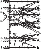
(c) Doubly top resonant

(d) Three top/antitop propagators

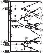
(e) $\mathrm{t}\bar{}\mathrm{t}$ intermediate state

(f) Singly top resonant

(g) Singly top resonant

(h) Non top resonant

Figure 1: Sample LO diagrams for the partonic channel $\mathrm{g}\mathrm{g}\to\mu^{-}\bar{\nu}_{\mu}\mathrm{e}^{+}\nu_{\mathrm{e}}\bar{}\mathrm{b}\mathrm{b}\bar{}\mathrm{b}\mathrm{b}$.

The diagram in Figure 1(d) contains one antitop and two top propagators. While both top propagators cannot be simultaneously resonant, each one becomes resonant in some part of phase space, corresponding to different on-shell processes, i.e. $\mathrm{t}\bar{}\mathrm{t}$ production with the subsequent decays $\mathrm{t}\to\nu_{\mathrm{e}}\mathrm{e}^{+}\mathrm{b}\bar{}\mathrm{b}\mathrm{b}$ and $\bar{}\mathrm{t}\to\bar{\nu}_{\mathrm{e}}\mathrm{e}^{-}\bar{}\mathrm{b}$ and $\bar{}\mathrm{t}\mathrm{t}\bar{}\mathrm{b}\mathrm{b}$ production with the subsequent decays $\mathrm{t}\to\nu_{\mathrm{e}}\mathrm{e}^{+}\mathrm{b}$ and $\bar{}\mathrm{t}\to\bar{\nu}_{\mu}\mu^{-}\bar{}\mathrm{b}$. On the other hand, the diagram in Figure 1(e) contributes only to $\mathrm{t}\bar{}\mathrm{t}$ production but not to $\bar{}\mathrm{t}\mathrm{t}\bar{}\mathrm{b}\mathrm{b}$ production, since there are no $\bar{}\mathrm{t}\mathrm{t}\bar{}\mathrm{b}\mathrm{b}$ intermediate states.

The computation is carried out in the 5-flavour scheme that assumes the bottom quarks to be massless throughout. All leptons and quarks (apart from the top quark) are thus taken to be massless. Also, all potentially resonant particles, i.e. top quark, W boson and Z boson, are treated within the complex-mass scheme [54, 55, 56], ensuring gauge invariance of all the amplitudes.

Double-pole approximation

Similar to Refs. [52, 13], in addition to the full computation we also perform a calculation based on a DPA. Note that the DPA is only applied to matrix elements, while the physical observables are calculated with off-shell kinematics. Specifically, we examine the tt-DPA which consists in retaining only contributions that feature two resonant top quarks and projecting the top-quark momenta on shell, apart from those in the denominators of the resonant propagators, which are kept off shell. At LO, the tt-DPA is based on the doubly-top-resonant contributions in the Born matrix element. More precisely, we include only those Feynman diagrams that contain both the decays $\mathrm{t}\to\nu_{\mathrm{e}}\mathrm{e}^{+}\mathrm{b}$ and $\bar{}\mathrm{t}\to\bar{\nu}_{\mu}\mu^{-}\bar{}\mathrm{b}$ as sub-diagrams, like those in Figures 1(a), 1(b), 1(c), and 1(d), but no diagrams with different top decays like the one in Figure 1(e). Moreover, only one of the bottoms, say bottom 1, is allowed as decay product of the top quark, while the other one, bottom 2, is not, i.e. diagrams with bottoms interchanged are not contained in the DPA. The same applies to the antibottoms with respect to the antitops. In addition, the resulting squared amplitudes from Recola are multiplied by a factor 4 to ensure the correct symmetry factors. The on-shell projection is performed in the same way as described for $\mathrm{t}\bar{}\mathrm{t}$ production in Ref. [52]. We note that some of the diagrams contributing to the DPA, e.g. the one in Figure 1(d), contain besides contributions to $\mathrm{t}\bar{}\mathrm{t}\mathrm{b}\bar{}\mathrm{b}$ production also doubly resonant contributions to $\mathrm{t}\bar{}\mathrm{t}$ production with the top (or antitop) decaying into $\mathrm{t}\to\nu_{\mathrm{e}}\mathrm{e}^{+}\mathrm{b}\bar{}\mathrm{b}\mathrm{b}$ (or $\bar{}\mathrm{t}\to\bar{\nu}_{\mu}\mu^{-}\bar{}\mathrm{b}\bar{}\mathrm{b}\mathrm{b}$). Diagrams like the one in Figure 1(e) that contain $\mathrm{t}\bar{}\mathrm{t}$ production but not $\mathrm{t}\bar{}\mathrm{t}\mathrm{b}\bar{}\mathrm{b}$ production as a subprocess are not included in the DPA. As opposed to a narrow-width approximation, in the DPA full spin correlations, off-shell propagators, as well as the full phase space are taken into account. In the tt-DPA calculation, we treat W and Z bosons in the complex-mass scheme.

At NLO the DPA is applied only to the virtual corrections, and also the doubly-resonant non-factorisable corrections following the algorithm of Refs. [57, 58, 59] transferred to QCD are included. All other contributions of orders $\mathcal{O}{\left(\alpha_{\mathrm{s}}^{4}\alpha^{4}\right)}$ and $\mathcal{O}{\left(\alpha_{\mathrm{s}}^{5}\alpha^{4}\right)}$, i.e. LO, real and subtraction terms, are kept exact.

Note that, as in the original DPA computations [51], in the past computations with MoCaNLO [52, 13, 60] the DPA (retaining resonant contributions and applying the on-shell projection) has also been applied to the I-operator in the integrated dipoles. It has been noticed [61] that when done in combination with small $\alpha_{\mathrm{dipole}}$ parameter [62], this tends to worsen the agreement with the full computation, as it treats large contributions in the subtracted and re-added real corrections that should cancel differently. Applying instead the DPA only to the virtual corrections, with IR singularities subtracted via an appropriate choice of regularisation parameters, avoids this mismatch and provides better agreement with the full calculation.

The DPA is constructed as a check of the full calculation and to provide a good approximation thereof. While a comparison of this approximation with the full calculation cannot yield quantitative results on off-shell top-quark effects, it nevertheless gives an indication on their size. In practice, the actual off-shell effects are often even larger, in particular, in specific regions of phase space.

Tools

The numerical integration has been carried out with the help of the multi-channel Monte Carlo integration program MoCaNLO. This code was developed for the integration of high-multiplicity processes involving top–antitop pairs and has proven to be particularly efficient for those and related processes [8, 52, 13, 53]. It relies on a multi-channel phase-space integration following Refs. [63, 54, 64].

All one-loop amplitudes in the 8-body phase space have been obtained from the matrix-element generator Recola2 [44, 45, 46, 47] in combination with the Otter library that is based on the on-the-fly reduction [65] and uses the stability improvements for hard kinematics described in Ref. [66]. By default, Otter uses double-precision scalar integrals provided by Collier [49, 50] and for exceptional phase-space points makes targeted use of multi-precision scalar integrals provided by OneLOop [67]. The computation of the virtual amplitudes has been carried out as well exclusively with the COLI branch of the Collier library, yielding perfect agreement. The infrared (IR) singularities in the real and virtual corrections are handled via the Catani–Seymour dipole subtraction formalism [68, 62]. We note that the partonic process $\mathrm{b}\mathrm{g}\to\mu^{-}\bar{\nu}_{\mu}\mathrm{e}^{+}\nu_{\mathrm{e}}\bar{}\mathrm{b}\mathrm{b}\bar{}\mathrm{b}\mathrm{b}\mathrm{b}$ involves 40 Catani–Seymour dipoles, while $\mathrm{g}\mathrm{g}\to\mu^{-}\bar{\nu}_{\mu}\mathrm{e}^{+}\nu_{\mathrm{e}}\bar{}\mathrm{b}\mathrm{b}\bar{}\mathrm{b}\mathrm{b}\mathrm{g}$ involves 30.

Validations

This computation builds on several previous computations for processes involving top–antitop pairs with MoCaNLO [8, 52, 13, 53, 36] which have themselves been thoroughly checked. Within the dipole-subtraction scheme, the variation of the $\alpha_{\mathrm{dipole}}$ parameter [62] that narrows the phase space to singular regions has been used. For representative channels a comparison of results for $\alpha_{\mathrm{dipole}}=1$ and $\alpha_{\mathrm{dipole}}=10^{-2}$ has revealed perfect agreement within statistical errors. The results presented below have been obtained using $\alpha_{\mathrm{dipole}}=10^{-2}$. Furthermore, independence on the IR-regulator parameter has been verified for representative channels, proving IR finiteness. Finally, the virtual corrections were computed with Recola2 both in the conventional ’t Hooft–Feynman gauge and within the Background-Field method using the two independent integral-reduction libraries Otter and Collier. Moreover, for the gluon-initiated process we verified that when replacing one of the gluon polarisation vectors at a time by its normalised four-momentum via $\epsilon^{\mu}_{\mathrm{g}}\to p_{\mathrm{g}}^{\mu}/p_{\mathrm{g}}^{0}$ only in the virtual amplitude, the corresponding contribution to the cross section integrates to a numerical zero at the relative level of $10^{-8}$. Finally, the calculation based on the DPA for the virtual corrections provides a further validation of the full NLO calculation.

2.3 Input parameters and event selection

Input parameters

The theoretical predictions presented here are for the LHC at $13\,\mathrm{TeV}$ centre-of-mass energy. The on-shell values for the masses and widths of the gauge bosons [69],

$$\begin{array}[b]{rcl@{\qquad}rcl}M_{\mathrm{W}}^{\rm os}&=&80.379\,\mathrm{GeV},&\Gamma_{\mathrm{W}}^{\rm os}&=&2.085\,\mathrm{GeV},\\ M_{\mathrm{Z}}^{\rm os}&=&91.1876\,\mathrm{GeV},&\Gamma_{\mathrm{Z}}^{\rm os}&=&2.4952\,\mathrm{GeV},\end{array}$$ (2.4)

are converted into pole masses according to [70]

$$M_{V}=M_{V}^{\rm os}/c_{V},\qquad\Gamma_{V}=\Gamma_{V}^{\rm os}/c_{V},$$

$$c_{V}=\sqrt{1+(\Gamma_{V}^{\rm os}/M_{V}^{\rm os})^{2}},\quad V=\mathrm{W},\mathrm{Z}.$$ (2.5)

The latter are used in the calculation. The top-quark mass and widths are fixed to

$$m_{\mathrm{t}}=173\,\mathrm{GeV},\qquad\Gamma_{\mathrm{t}}^{\rm LO}=1.443303\,\mathrm{GeV},\qquad\Gamma_{\mathrm{t}}^{\rm NLO}=1.3444367445\,\mathrm{GeV}.$$ (2.6)

The top-quark width at LO has been computed based on the formulas of Ref. [71], while the NLO QCD value has been obtained upon applying the relative QCD corrections of Ref. [72] to the LO width. The LO top width is utilised for the LO computation, while the NLO one is employed in the NLO calculation (including the Born contributions).

Concerning the electromagnetic coupling $\alpha$, the $G_{\mu}$ scheme is applied, where $\alpha$ is fixed from the Fermi constant,

$$\alpha_{G_{\mu}}=\frac{\sqrt{2}}{\pi}G_{\mu}M_{\mathrm{W}}^{2}\left(1-\frac{M_{\mathrm{W}}^{2}}{M_{\mathrm{Z}}^{2}}\right),$$ (2.7)

with

$$G_{\mu}=1.16638\times 10^{-5}\,\mathrm{GeV}^{-2}.$$ (2.8)

The sets of parton distribution functions (PDF) NNPDF31 LO and NNPDF31 NLO with $\alpha_{\mathrm{s}}=0.118$ [73] have been used at LO and NLO, respectively. The values of $\alpha_{\mathrm{s}}$ for the dynamical scales have been taken from the PDF sets which are interfaced through LHAPDF [74, 75]. Accordingly, a variable-flavour-number scheme with at most 5 flavours is used for the running of $\alpha_{\mathrm{s}}$.

The renormalisation and factorisation scales, $\mu_{\mathrm{ren}}$ and $\mu_{\mathrm{fact}}$, are set equal to

$$\mu_{0}=\frac{1}{2}\Biggl{[}\Biggl{(}p^{\mathrm{miss}}_{{\mathrm{T}}}+\sum_{i=\ell,{\rm J}}E_{{\mathrm{T}},i}\Biggr{)}+2m_{\mathrm{t}}\Biggr{]}^{1/2}\Biggl{(}\sum_{i={\rm J}}E_{{\mathrm{T}},i}\Biggr{)}^{1/2},$$ (2.9)

where $p^{\mathrm{miss}}_{{\mathrm{T}}}$ is the transverse component of the vector sum of the two neutrino momenta and J denotes all bottom and light jets after jet clustering. The transverse energy $E_{{\mathrm{T}},i}$ of the other particles is defined as $E_{{\mathrm{T}},i}=\sqrt{p_{{\mathrm{T}},i}^{2}+m_{i}^{2}}$, where $m_{i}^{2}$ is the invariant-mass squared of the object considered (which can be a jet resulting from parton recombination and is thus not necessarily zero). Note that this choice of scale has the property not to refer explicitly to a top quark, as it has been done so far in the literature. While the first factor in Eq. (2.9) serves as a proxy for the typical momentum transfer in the strong couplings of the top quarks, the second one mimics the one in the couplings of the bottom quarks in the process. The choice can be viewed as a modification of the renormalisation scales used in Refs. [23, 24, 28] avoiding identification of the top quarks.

Event selection

The event selection is generic and assumes a resolved topology (as opposed to a boosted kinematics). Quarks and gluons are clustered using the anti-$k_{\mathrm{T}}$ algorithm [76] with a jet-resolution parameter $R=0.4$. Concerning the flavour, the recombination rules read,

• $\mathrm{j}+\mathrm{j}\to\mathrm{j}$,

• $\mathrm{j}_{\rm b}+\mathrm{j}\to\mathrm{j}_{\rm b}$,

• $\mathrm{j}_{\rm b}+\mathrm{j}_{\rm b}\to\mathrm{j}$,

where the bottom jet $\mathrm{j}_{\rm b}$ contains at least one $\mathrm{b}$ or $\bar{}\mathrm{b}$ quark, while $\mathrm{j}$ is a light jet. The last combination is implemented in order to account for a proper treatment of the singularity originating from gluon splitting into pairs of bottom–antibottom quarks and effectively leads to the elimination of events where the bottom and antibottom quarks are collinear and thus recombined into one jet. For each bottom jet and charged lepton, a cut on its transverse momentum and its rapidity is applied,

$$p_{{\mathrm{T}},\mathrm{j}_{\mathrm{b}}}>{} 25\,\mathrm{GeV},\qquad|y_{\mathrm{j}_{\mathrm{b}}}|<2.5,$$

$$p_{{\mathrm{T}},\ell}>{} 20\,\mathrm{GeV},\qquad|y_{\ell}|<2.5,$$ (2.10)

where $\ell=\mathrm{e}^{+},\mu^{-}$. Finally, we require at least 4 bottom jets, a positron, and a muon passing all these cuts in the final state.

3 Numerical results

3.1 Cross sections

The LO and NLO cross sections obtained from the full computation read

$$\sigma_{\rm LO}=5.203(4)^{+60\%}_{-35\%}{\,\text{fb}}\qquad{\rm and}\qquad\sigma_{\rm NLO}=10.31(8)^{+18\%}_{-21\%}{\,\text{fb}},$$ (3.1)

respectively. The digits in parentheses indicate the numerical Monte Carlo errors on the predictions. The superscript and subscript represent the percentage scale variations. We use the conventional 7-point scale variation, i.e. we calculate the quantities for the following pairs of renormalisation and factorisation scales,

$$(\mu_{\mathrm{ren}}/\mu_{0},\mu_{\mathrm{fact}}/\mu_{0})=(0.5,0.5),(0.5,1),(1,0.5),(1,1),(1,2),(2,1),(2,2)$$ (3.2)

with the central scale defined in Eq. (2.9) and use the resulting envelope. The first observation is that the corrections are substantial and amount to $97.8\%$ for the central scale, i.e. the $K$-factor is $1.98$. The large $K$-factor is related to our scale choice (2.9) which results in somewhat larger scales than usual. The dependence of the results on the scale choice is shown in Figure 2 for the case when both the renormalisation and factorisation scales are set to a common value.

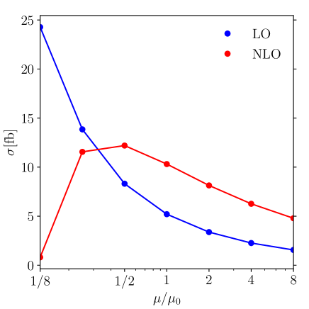
Figure 2: Cross section at LO and NLO in fb for the process $\mathrm{p}\mathrm{p}\to\mu^{-}\bar{\nu}_{\mu}\mathrm{e}^{+}\nu_{\mathrm{e}}\bar{}\mathrm{b}\mathrm{b}\bar{}\mathrm{b}\mathrm{b}$ at $\sqrt{s}=13\,\mathrm{TeV}$ as a function of the scale $\mu$, which refers to both the factorisation and renormalisation scales. The central scale $\mu_{0}$ is defined in Eq. (2.9).

Based on these results, choosing $\mu_{0}/2$ as central scale might be preferable, as it is closer to the maximum of the NLO curve and gives rise to smaller NLO QCD corrections ($K=1.47$) in agreement with results for on-shell top quarks in the literature [23, 78, 28, 29]. In any case, the inclusion of NLO QCD corrections significantly reduces the size of the scale uncertainty from $[+60\%,-35\%]$ to $[+18\%,-21\%]$.

Table 1 shows the cross sections of the different partonic channels.

Ch.	$\sigma_{\rm LO}$ [fb]	$\sigma_{\rm NLO}$ [fb]	$K$-factor	$\delta[\%]$
$\mathrm{g}\mathrm{g}$	$4.861(4)$	$9.95(8)$	$2.05$	$96.4$
${q}\bar{{q}}$	$0.3298(1)$	$0.43(1)$	$1.30$	$4.2$
$\mathrm{b}\bar{\mathrm{b}}$	$0.00742(1)$	$0.017(2)$	$2.29$	$0.16$
$\mathrm{g}{q}/\mathrm{g}\bar{{q}}$	-	$-0.19(2)~{}$	-	$-1.8~{}$
$\mathrm{g}\mathrm{b}/\mathrm{g}\bar{\mathrm{b}}$	-	$0.094(2)$	-	$0.91$
$\mathrm{b}\mathrm{b}$	$0.00263(1)$	$0.0072(9)$	$2.76$	$0.070$
$\bar{}\mathrm{b}\bar{}\mathrm{b}$	$0.00262(1)$	$0.0057(8)$	$2.18$	$0.055$
$\mathrm{p}\mathrm{p}$	$5.203(4)$	$10.31(8)$	$1.98$	$100$

Table 1: Fiducial cross sections at LO and NLO in fb for the process $\mathrm{p}\mathrm{p}\to\mu^{-}\bar{\nu}_{\mu}\mathrm{e}^{+}\nu_{\mathrm{e}}\bar{}\mathrm{b}\mathrm{b}\bar{}\mathrm{b}\mathrm{b}$ with its corresponding sub-channels at $\sqrt{s}=13\,\mathrm{TeV}$. The channels for light quark flavours ${q}=\mathrm{u},\mathrm{d},\mathrm{c},\mathrm{s}$ are grouped into one category. The quark–gluon channels denoted by $\mathrm{g}{q}/\mathrm{g}\bar{{q}}$ appear only at NLO in the real corrections. The contributions involving bottom quarks in the initial state, $\mathrm{b}\bar{\mathrm{b}}$, $\mathrm{g}\mathrm{b}/\mathrm{g}\bar{\mathrm{b}}$, $\mathrm{b}\mathrm{b}$, and $\bar{}\mathrm{b}\bar{\mathrm{b}}$, are shown separately. The hadronic cross section is listed in the last line of the table dubbed $\mathrm{p}\mathrm{p}$. The $K$-factors are defined as $K=\sigma_{\rm NLO}/\sigma_{\rm LO}$, and $\delta$ represents the contributions relative to the full NLO result. The integration errors of the last digits are given in parentheses.

As usual at the LHC, the gluon-initiated contributions largely dominate the partonic cross section. For example, at LO the $\mathrm{g}\mathrm{g}$ channel represents $96.4\%$ of the hardonic cross section, while the ${q}\bar{{q}}$ channels with $q=\mathrm{u},\mathrm{d},\mathrm{c},\mathrm{s}$ give $4.2\%$ and $\mathrm{b}\bar{\mathrm{b}}$, $\mathrm{b}\mathrm{b}$, and $\bar{}\mathrm{b}\bar{\mathrm{b}}$, only $0.16\%$, $0.070\%$, and $0.055\%$, respectively. The $\mathrm{g}\mathrm{g}$ and ${q}\bar{{q}}$ channels get NLO QCD $K$-factors $2.05$ and $1.30$, respectively. Such differences have already been observed for several top–antitop production processes (see for instance Refs. [21, 8, 53]). We note that for the bottom-induced channels, the $K$-factor is even higher and ranges between $2.18$–$2.76$. However, these contributions are greatly suppressed by their (anti-)bottom-quark PDFs and are below $0.3\%$ of the total cross section at both LO and NLO. At NLO, new partonic channels are opening up. The $\mathrm{g}{q}/\mathrm{g}\bar{{q}}$ channels yield rather small negative corrections (of the order of $-1.8\%$ of the total NLO cross section), while the $\mathrm{g}\mathrm{b}/\mathrm{g}\bar{\mathrm{b}}$ contribution is positive and reaches $+0.9\%$. Overall the NLO corrections are dominated by the ones of the $\mathrm{g}\mathrm{g}$ channel to raise a $K$-factor of $1.98$.

The cross sections in the tt-DPA, retaining only doubly-top-resonant contributions as specified in Section 2.2, read

$$\sigma_{\rm LO}^{\rm DPA}=5.029(2)^{+60\%}_{-35\%}{\,\text{fb}}\qquad{\rm and}\qquad\sigma_{\rm NLO}^{\rm DPA}=10.23(8)^{+19\%}_{-21\%}{\,\text{fb}}.$$ (3.3)

These values should be compared to the ones of the full computation in Eq. (3.1). First, the scale variation is essentially the same as in the full calculation, indicating that the functional dependence of the cross sections on the renormalisation and factorisation scales is not significantly modified. Looking at the central values, one observes that the tt-DPA is lower than the full computation by $3.3\%$ at LO. At NLO, the difference between the two cross sections ($0.8\%$) is of the order of the integration error which is $0.7\%$. This is due to the way the NLO DPA is constructed (see Section 2.2). While the full LO and real contributions are used, only the virtual contributions are computed in the pole approximation. Since the virtual corrections amount to about $30\%$, the expected error of the tt-DPA at NLO is about $30\%$ of the expected error at LO, i.e. $0.3\Gamma_{\mathrm{t}}/m_{\mathrm{t}}\approx 0.25\%$.

For $\mathrm{t}\bar{}\mathrm{t}$ production, finite-width effects at the level of one percent have been found by comparing the off-shell calculation with the narrow-top-width limit in Refs. [79, 80, 81]. It is instructive to perform a similar analysis for the process (2.1). To this end, we determine the corresponding narrow-top-width limit in LO as in Ref. [80] by a numerical extrapolation,

$$\bar{\sigma}(\Gamma_{\mathrm{t}})=\sigma(\Gamma_{\mathrm{t}})\left(\frac{\Gamma_{\mathrm{t}}}{\Gamma_{\mathrm{t}}^{\mathrm{phys}}}\right)^{2}$$

in the range $0<\Gamma_{\mathrm{t}}<\Gamma_{\mathrm{t}}^{\mathrm{phys}}$, where $\Gamma_{\mathrm{t}}^{\mathrm{phys}}$ is the physical top-quark width from Eq. (2.6), for the dominating $\mathrm{g}\mathrm{g}$ channel. The factor $\left(\Gamma_{\mathrm{t}}/\Gamma_{\mathrm{t}}^{\mathrm{phys}}\right)^{2}$ ensures that effective top-decay branching ratios remain constant in the limit. In Figure 3 we show results of this extrapolation for the full calculation, for the DPA, and for a calculation (res $\mathrm{t}\bar{}\mathrm{t}$) where we take into account the same subset of diagrams as in the DPA but do not perform the on-shell projection.

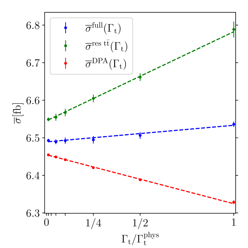
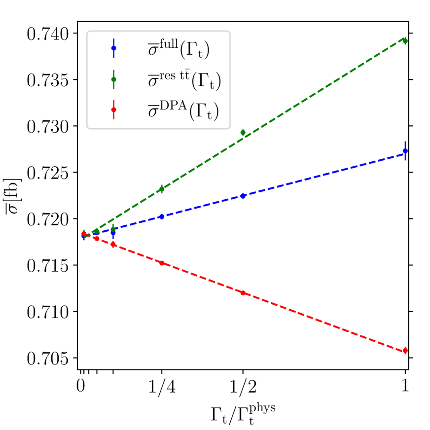
Figure 3: . Extrapolation of fiducial cross sections to the limit $\Gamma_{\mathrm{t}}\to 0$ for the gluon-induced channel $\mathrm{g}\mathrm{g}\to\mu^{+}\nu_{\mu}\mathrm{e}^{+}\nu_{\mathrm{e}}\bar{}\mathrm{b}\mathrm{b}\bar{}\mathrm{b}\mathrm{b}$ for a fixed scale $\mu_{\mathrm{ren}}=\mu_{\mathrm{fact}}=173.34\,\mathrm{GeV}$. The left plot shows results for our default setup (but fixed scale) while in the plot on the right we imposed an additional invariant-mass cut $M_{\mathrm{b}\mathrm{b}}>110\,\mathrm{GeV}$.

This analysis yields two interesting results: First, the difference between the DPA and the full calculation is larger than the difference between the full calculation and its narrow-width approximation. This indicates that contributions of non-resonant diagrams and finite-width effects of the resonant diagrams cancel to some extent, and the generic accuracy of on-shell calculations is worse. Second, the narrow-width limits of the three calculations do not agree, but differ at the level of one percent, the size of finite-width effects. The origin of these differences are contributions of resonant top or antitop quarks that decay via $\mathrm{t}\to\nu_{\mathrm{e}}\mathrm{e}^{+}\mathrm{b}\bar{}\mathrm{b}\mathrm{b}$ or $\bar{}\mathrm{t}\to\bar{\nu}_{\mu}\mu^{-}\bar{}\mathrm{b}\bar{}\mathrm{b}\mathrm{b}$. While some of these contributions, e.g. Figure 1(d), are included in the subset of diagrams selected for the DPA, others, e.g. Figure 1(e), are not. This demonstrates that the narrow-width limit of the full calculation differs by contributions of the order of $\Gamma_{\mathrm{t}}/m_{\mathrm{t}}$ from an on-shell calculation of $\mathrm{t}\bar{}\mathrm{t}\mathrm{b}\bar{}\mathrm{b}$ production with subsequent top decays. The construction of a narrow-width approximation based on on-shell calculations that takes into account all these top resonances would be non-trivial. While the extrapolation was performed at LO, the same kind of features persists in an NLO calculation.

The situation is different for $\mathrm{t}\bar{}\mathrm{t}$ production, where no extra top resonances are present. We verified with our codes that for $\mathrm{g}\mathrm{g}\to\mu^{-}\bar{\nu}_{\mu}\mathrm{e}^{+}\nu_{\mathrm{e}}\bar{}\mathrm{b}\mathrm{b}$ the DPA and the approximation “res $\mathrm{t}\bar{}\mathrm{t}$” based on resonant $\mathrm{t}\bar{}\mathrm{t}$ diagrams approach the same value in the narrow-top-width limit. Also for $\mathrm{t}\bar{}\mathrm{t}\mathrm{b}\bar{}\mathrm{b}$ production the cross sections for the different approximations in the narrow-top-width limit coincide, if one eliminates the resonances related to $\mathrm{t}\to\nu_{\mathrm{e}}\mathrm{e}^{+}\mathrm{b}\bar{}\mathrm{b}\mathrm{b}$ or $\bar{}\mathrm{t}\to\bar{\nu}_{\mu}\mu^{-}\bar{}\mathrm{b}\bar{}\mathrm{b}\mathrm{b}$ decays with additional cuts. This is demonstrated in the right plot in Figure 3, where we imposed the additional cut $M_{\mathrm{b}\mathrm{b}}>110\,\mathrm{GeV}$ on all pairs of bottom and/or antibottom jets.

3.2 Differential distributions

Turning to differential distributions, several physical observables are shown in Figures 4–6. While in the upper panels, the absolute predictions at LO and NLO QCD in the full and in the tt-DPA are displayed, the two lower panels show the same contributions with respect to different normalisations. In these panels the error bars represent the numerical Monte Carlo errors. In the middle insets the size of the QCD corrections in the full computation and in the tt-DPA is compared. Finally, the lower insets illustrate the quality of the approximate computation by normalising the tt-DPA to the full computation at both LO and NLO QCD.

In Figure 4, we present the distributions in the transverse momentum and the invariant mass of the bottom–antibottom pair that does not originate from the top-quark decay. In a $\mathrm{t}\bar{}\mathrm{t}\mathrm{H}$ analysis with $\mathrm{H}\to\mathrm{b}\bar{}\mathrm{b}$, this pair of bottom jets corresponds to the background of the decay products of the Higgs boson. More precisely, the bottom jets are identified as originating from a top quark by maximising the likelihood function $\mathcal{L}$, defined as a product of two Breit–Wigner distributions corresponding to the top-quark and antitop-quark propagators,

$$\mathcal{L}_{ij}=\frac{1}{\left(p^{2}_{\mu^{-}\bar{\nu}_{\mu}\mathrm{b}_{i}}-m_{\mathrm{t}}^{2}\right)^{2}+\left(m_{\mathrm{t}}\Gamma_{\mathrm{t}}\right)^{2}}\;\frac{1}{\left(p^{2}_{\mathrm{e}^{+}\nu_{\mathrm{e}}\mathrm{b}_{j}}-m_{\mathrm{t}}^{2}\right)^{2}+\left(m_{\mathrm{t}}\Gamma_{\mathrm{t}}\right)^{2}},$$ (3.4)

where the momenta $p_{abc}$ are defined as $p_{abc}=p_{a}+p_{b}+p_{c}$. The combination of bottom jets $\{\mathrm{b}_{i},\mathrm{b}_{j}\}$ that maximises this function defines the two bottom jets originating from top quarks. From the 2 or 3 bottom jets left in the event, the two hardest ones, i.e. those with highest transverse momenta, define the bottom–antibottom pair that does not originate from the top-quark decay and whose transverse-momentum and invariant-mass distributions are shown in Figure 4.

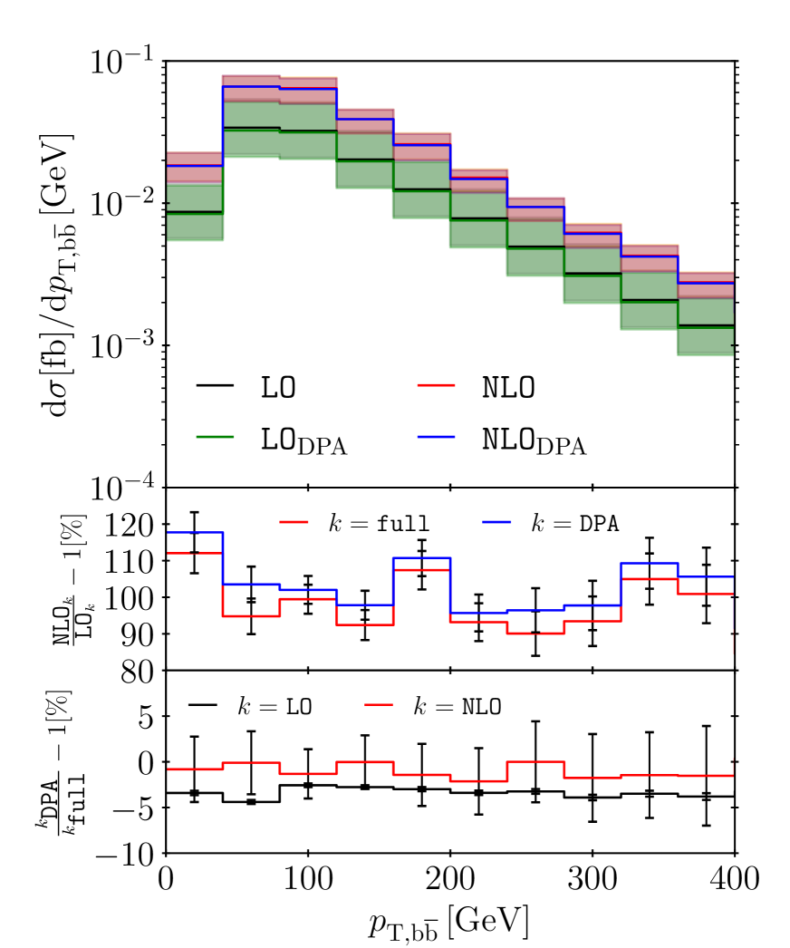
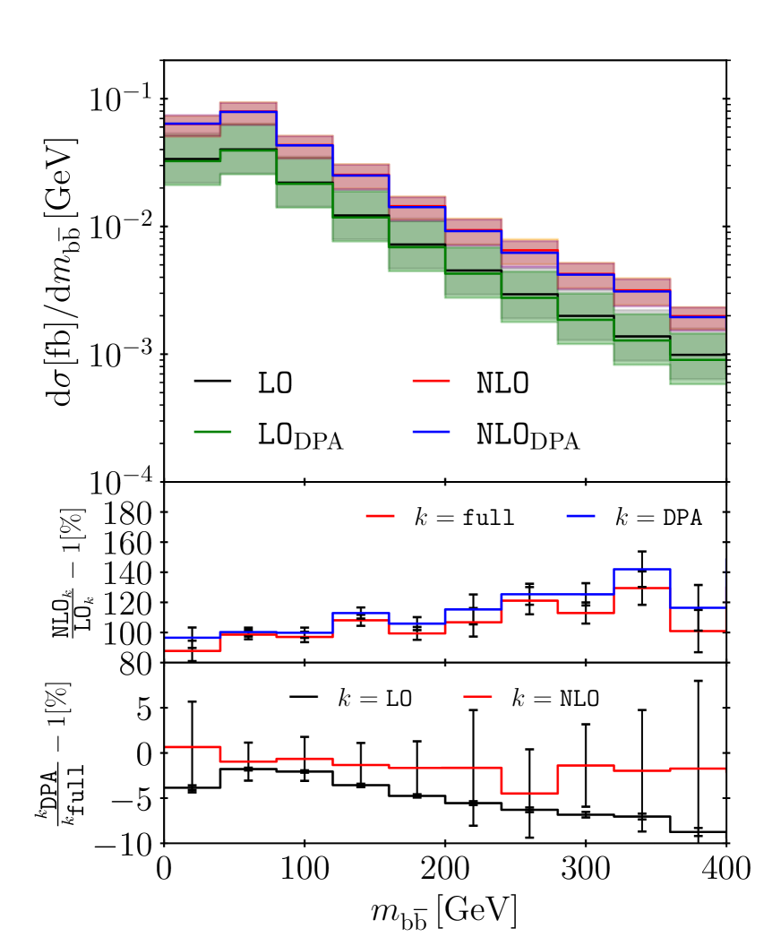
Figure 4: Differential distributions at LO and NLO for $\mathrm{p}\mathrm{p}\to\mu^{+}\nu_{\mu}\mathrm{e}^{+}\nu_{\mathrm{e}}\bar{}\mathrm{b}\mathrm{b}\bar{}\mathrm{b}\mathrm{b}$: transverse momentum of the two bottom jets not originating from a top quark, and invariant mass of the two bottom jets not originating from a top quark.

The distribution in the transverse momentum of the two bottom jets not coming from a top decay shows rather stable corrections around $100\%$ apart from low transverse momentum, where the QCD corrections reach $110\%$. The difference between the full calculation and the one in DPA does not show significant variations over the phase space neither at LO nor at NLO QCD but is largely inherited from the fiducial cross section. In particular, the difference between the tt-DPA and the full calculation at NLO is within the integration errors, as for all following distributions. The distribution in the invariant mass of the bottom–antibottom pair, on the other hand, exhibits larger variations between the full computation and the tt-DPA one at LO. The difference between the two computations is about $4\%$ in the first bin, decreases to a few per cent around $100\,\mathrm{GeV}$ where the bulk of the cross section is located, and increases to almost $10\%$ at $400\,\mathrm{GeV}$. The additional contributions not contained in the tt-DPA increase the cross section. The largest effects appear for small $m_{\mathrm{b}\bar{}\mathrm{b}}$, a region that is enhanced by $\mathrm{b}\bar{}\mathrm{b}$ pairs resulting from virtual gluons (for instance Figure 1(f)), and for large invariant masses, where diagrams with bottom quarks coupling directly to the incoming gluons give sizeable contributions (for instance Figure 1(g)). The QCD corrections tend to grow when going to higher invariant masses. This is in contrast to the results of on-shell computations (see Figures 6 and 17 of Ref. [23]), where the relative corrections to the invariant-mass distribution tend to decrease with increasing invariant mass. This is most likely due to the different scale choices in the on-shell and off-shell calculations, where the scales in the latter tend to be higher. We mention that the two distributions in Figure 4 are the only ones that can be qualitatively compared with results of the literature where stable top quarks are used [23, 24, 28]. Since these computations are, however, done with different event selections and scale choices, a direct comparison is rather difficult. The transverse-momentum distribution is given as well in Figure 10 of Ref. [23] but with a cut of $100\,\mathrm{GeV}$ on the invariant mass of the two bottom jets. Nevertheless, the differential $K$-factor is flat for this distribution above $50\,\mathrm{GeV}$ both in the off-shell and on-shell calculation.

In Figure 5, the distribution in the transverse momentum of the second-hardest b jet is shown.

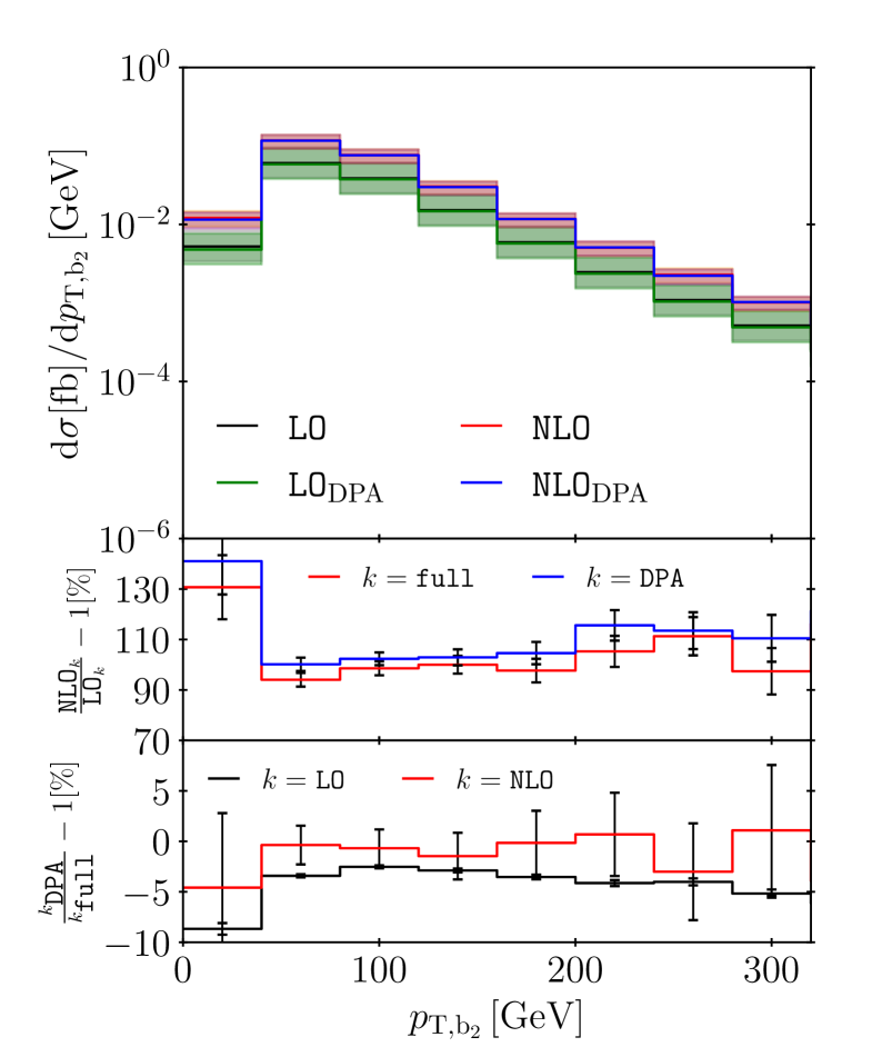
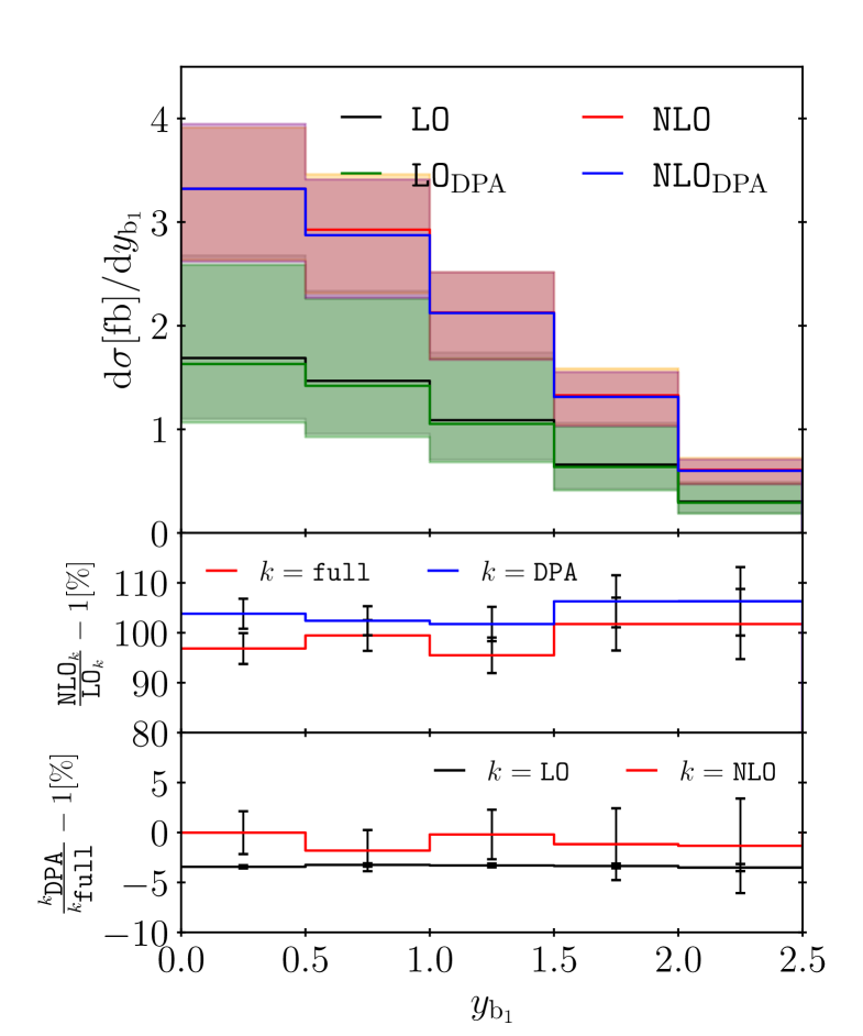
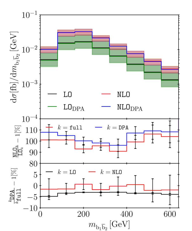
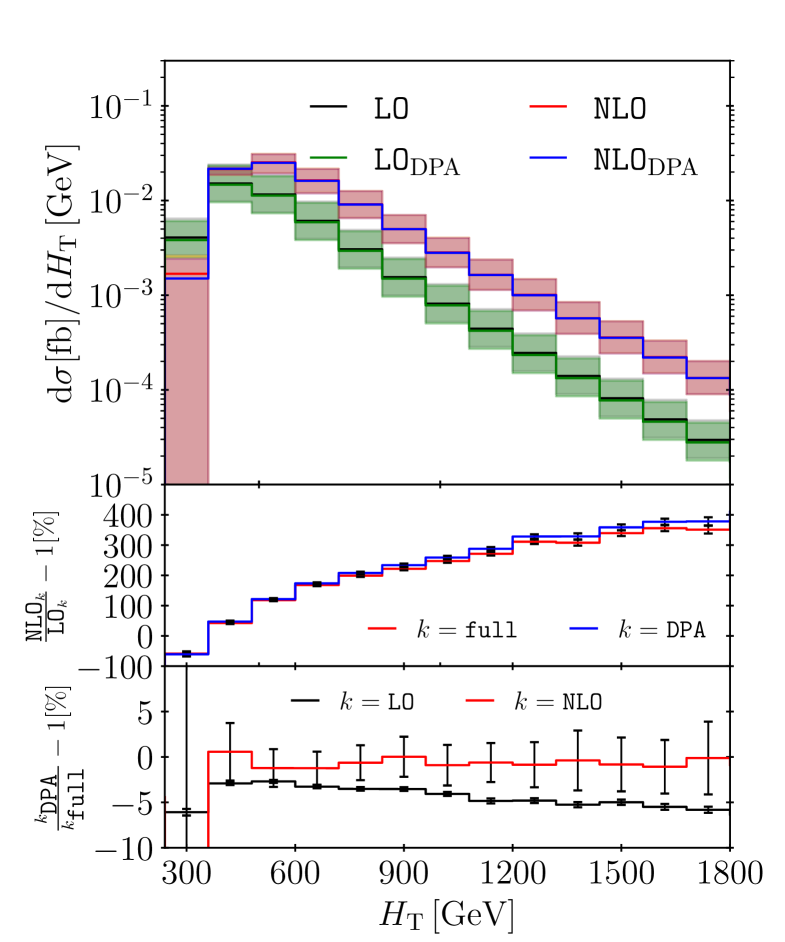
Figure 5: Differential distributions at LO and NLO for $\mathrm{p}\mathrm{p}\to\mu^{+}\nu_{\mu}\mathrm{e}^{+}\nu_{\mathrm{e}}\bar{}\mathrm{b}\mathrm{b}\bar{}\mathrm{b}\mathrm{b}$: transverse momentum of the second-hardest b jet, rapidity of the hardest b jet, invariant mass of the hardest and second-hardest b jet, and $H_{\rm T}$ observable (see text for definition).

The full corrections are large (about $130\%$) at low transverse momentum, then become smaller to finally reach roughly $100\%$ at $300\,\mathrm{GeV}$. Such a behaviour has already been observed in top–antitop production in the lepton+jets channel for the transverse momentum of the hardest b jet [53]. The large corrections were attributed to real radiations that take away momentum of the final-state particles. The effect of non-doubly-resonant top quarks is rather clear in this distribution at LO. The tt-DPA deviates from the full computation by almost $10\%$ in the first bin. The difference is minimal at $100\,\mathrm{GeV}$ but always between $2\%$ and $5\%$. This indicates significant non-doubly-resonant contributions that might originate from multi-peripheral diagrams where the bottom quarks couple directly to the incoming gluons (Figure 1(g)). Moreover, while bottom jets resulting from top quark decays tend to have transverse momenta of the order of the top mass, this is not the case for bottom jets in general. Looking at the distributions in the transverse momentum of the other b jets (not shown here), the difference between the tt-DPA and the full computation is reduced at low transverse momenta of the third and fourth hardest b jet, but enhanced for the hardest one. In contrast to the case of the hardest and second hardest b jets, for the third and fourth hardest b jets these configurations receive also contributions with doubly-resonant top quarks that are included in the tt-DPA. At NLO, the differences are within integration errors owing to the fact that the DPA is only applied to the virtual amplitudes. For the distribution in the rapidity of the hardest b jet, the full and the approximate computation have the same qualitative behaviour. The full NLO QCD corrections are essentially flat in this distribution. They are a bit above $+100\%$ at rapidity $2.5$ and slightly below $+100\%$ in the central region. The distribution in the invariant mass of the two hardest bottom jets is depicted in the bottom left of Figure 5. These bottom jets can either originate from a top-quark decay or are produced directly. The corrections tend to be larger at low and large invariant mass ($100\%$ at $0\,\mathrm{GeV}$ and $105\%$ at $600\,\mathrm{GeV}$) and reach a minimum around $300\,\mathrm{GeV}$ of $95\%$. The quality of the tt-DPA is rather good in this observable in the sense that no significant shape distortion is observed and only a difference in the overall normalisation is present. The last plot in Figure 5 concerns the distribution in $H_{\rm T}$, defined as

$$H_{\rm T}=p^{\mathrm{miss}}_{{\mathrm{T}}}+\sum_{i=\mathrm{e}^{+},\mu^{-},\mathrm{j}_{\mathrm{b}}}E^{i}_{{\mathrm{T}}}.$$ (3.5)

This observable is interesting because it gives an estimate of the typical scale of the process. This is the reason why it enters the definition of the renormalisation and factorisation scale in Eq. (2.9). Note that as opposed to Eq. (2.9), here only the four hardest bottom jets fulfilling the event selection in Eq. (2.10) are taken into account. While the corrections are of the usual size for low values of this quantity, they steadily increase to exceed $300\%$ above $1200\,\mathrm{GeV}$. Such an effect has already been observed for top-pair production [80]. The quality of the tt-DPA is at the level of $-3\%$ at LO around the maximum of the distribution near $500\,\mathrm{GeV}$. Above and below, the difference tends to increase: in the first non-trivial bin it amounts to around $-6\%$, while at high values it steadily reaches $-6\%$ at $1.8\,\mathrm{TeV}$.

The final set of distributions shown in Figure 6 deals with leptonic observables.

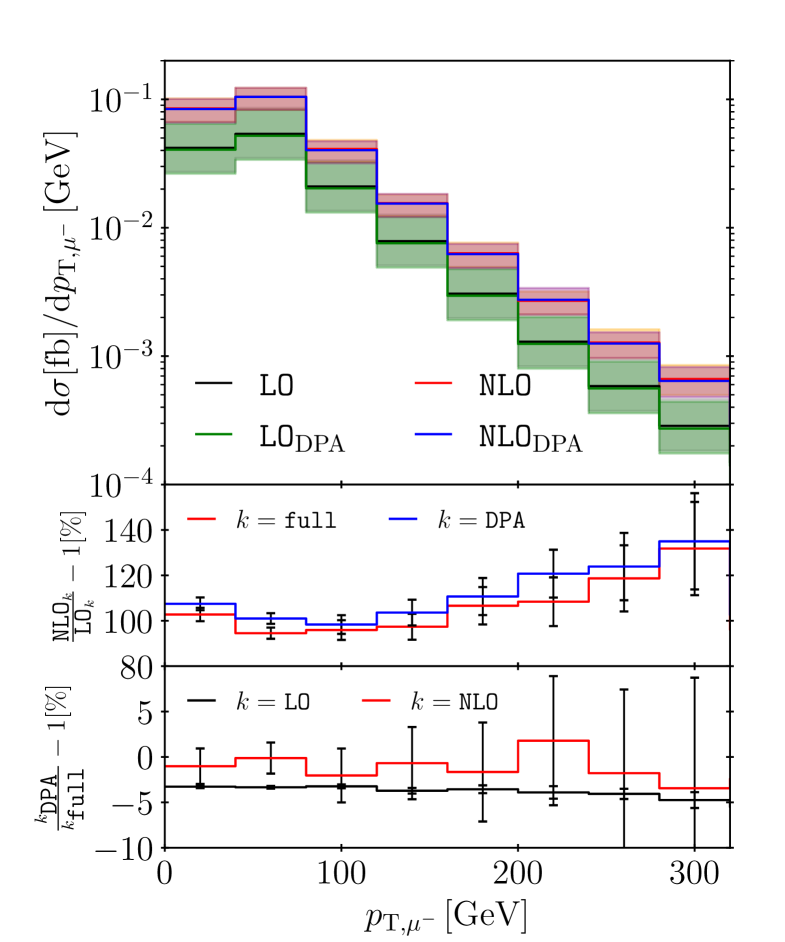
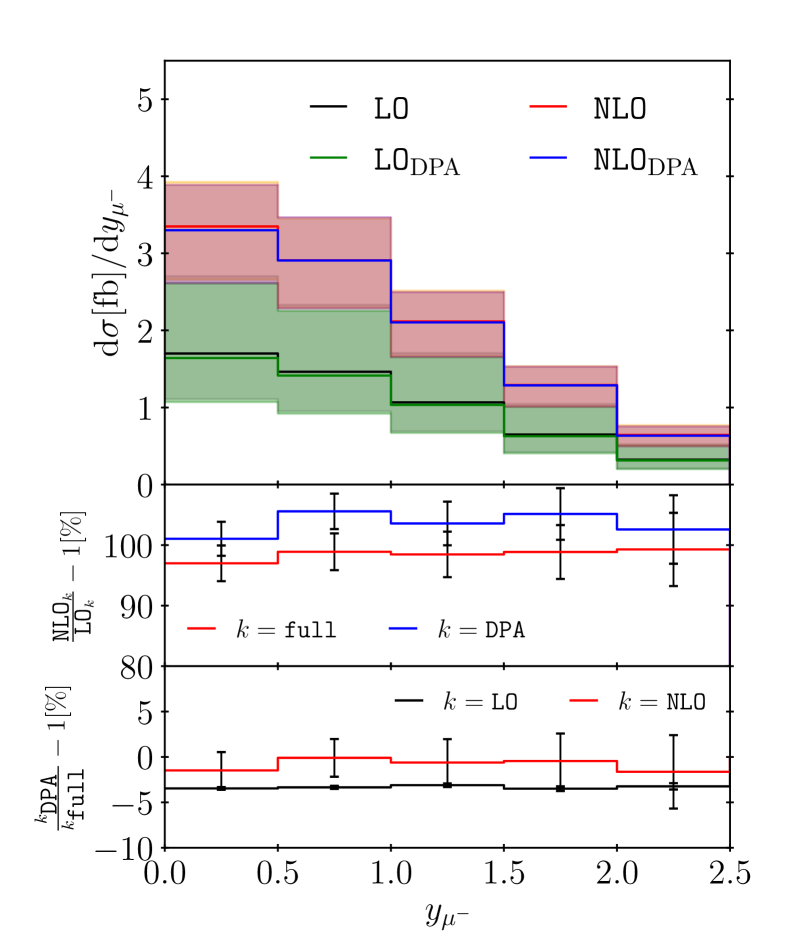
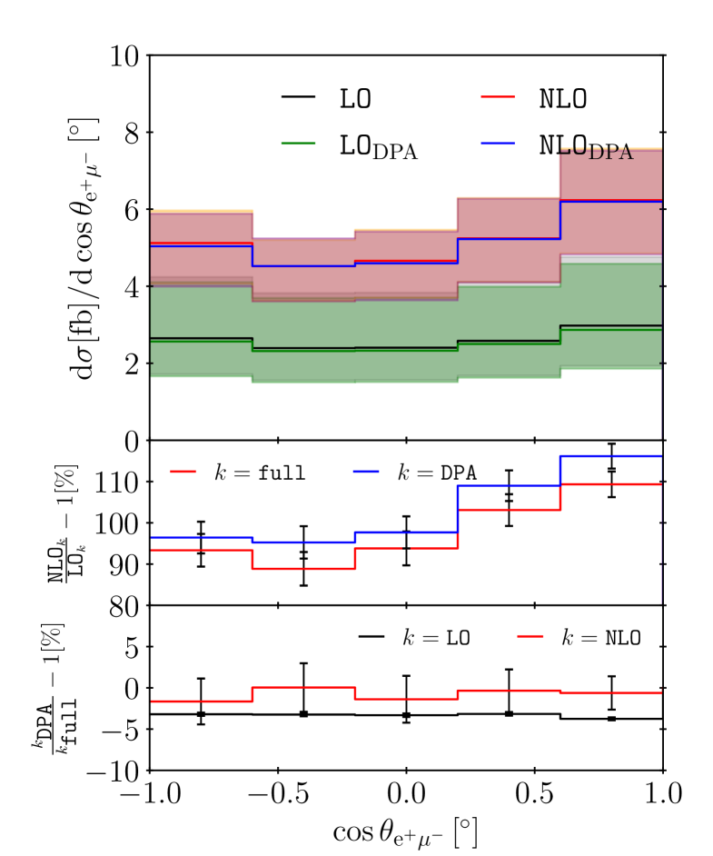
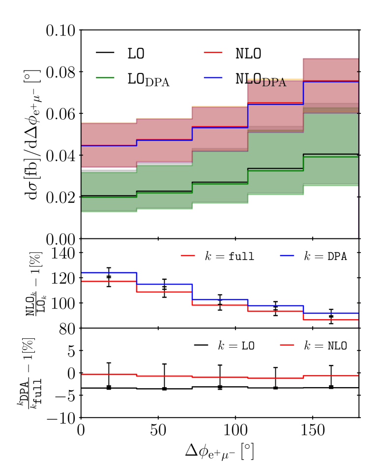
Figure 6: Differential distributions at LO and NLO for $\mathrm{p}\mathrm{p}\to\mu^{+}\nu_{\mu}\mathrm{e}^{+}\nu_{\mathrm{e}}\bar{}\mathrm{b}\mathrm{b}\bar{}\mathrm{b}\mathrm{b}$: transverse momentum of the muon, rapidity of the muon, cosine of the angle between the muon and the positron, and azimuthal-angle distance between the muon and the positron.

The corrections to the distribution in the transverse momentum of the muon are larger in the first bin, reach a minimum around $60\,\mathrm{GeV}$ and exceed $130\%$ towards high transverse momentum. In the same way, the disagreement between the full computation and the tt-DPA at LO tends to increase slowly from $3\%$ to $5\%$ when going to large momenta. Similarly to the distribution in the rapidity of the hardest bottom jet, the one of the muon also does not feature significant shape distortions in the QCD corrections. The full corrections are, to a large extent, inherited from the total cross section. The difference between the tt-DPA and the full calculation is flat over the kinematic range shown for this observable. For the distribution in the cosine of the angle between the muon and positron, the corrections generally tend to increase with $\cos\theta_{\mathrm{e}^{+}\mu^{-}}$, ranging between $90\%$ and $110\%$. The difference between the tt-DPA and the full computations is also flat. At last, we show the distribution in the azimuthal angle between the two leptons. The corrections are at the level of $120\%$ at zero degree and steadily decrease to $90\%$ in the back-to-back configuration. Again, the shape of the tt-DPA computation is quite similar to the one of the full calculation over the full range.

4 Conclusion

In this article we have presented the first full NLO QCD computation for $\mathrm{p}\mathrm{p}\to\mu^{-}\bar{\nu}_{\mu}\mathrm{e}^{+}\nu_{\mathrm{e}}\bar{}\mathrm{b}\mathrm{b}\bar{}\mathrm{b}\mathrm{b}$ at order $\mathcal{O}{\left(\alpha_{\mathrm{s}}^{5}\alpha^{4}\right)}$ at the LHC. This final state is of particular interest as it is shared with $\mathrm{p}\mathrm{p}\to\mathrm{t}\bar{}\mathrm{t}\mathrm{H}\bigl{(}\to\mathrm{b}\bar{}\mathrm{b}\bigr{)}$ which is key for the extraction of Higgs coupling to top quarks. The present computation is carried out with full tree and one-loop matrix elements and, thus, includes all off-shell and non-resonant contributions. It therefore goes beyond the state of the art of fixed-order computations, which focused so far on the description of the $\mathrm{t}\bar{}\mathrm{t}\mathrm{b}\bar{}\mathrm{b}$ process with stable top quarks. In addition to the phenomenological relevance, the calculation constitutes a significant progress in complexity as it is the first full NLO QCD computation for a $2\to 8$ process with 6 external strongly-interacting particles. Along with the full computation, we also provide predictions in a double-pole approximation which retains only doubly-resonant top contributions in the virtual corrections. Since the Feynman diagrams of the considered process include also resonant top and antitop quarks that are not related to on-shell production of $\mathrm{t}\bar{}\mathrm{t}\mathrm{b}\bar{}\mathrm{b}$ and subsequent top decays, the narrow-width limit of the full calculation differs from an on-shell calculation with subsequent decays, i.e. $\mathrm{p}\mathrm{p}\to\mathrm{t}\bar{}\mathrm{t}\mathrm{b}\bar{}\mathrm{b}$ followed by $\mathrm{t}\to\mu^{-}\bar{\nu}_{\mu}\mathrm{b}$ and $\bar{}\mathrm{t}\to\mathrm{e}^{+}\nu_{\mathrm{e}}\bar{}\mathrm{b}$, by terms of the order of the top width. Recent analyses have revealed differences between various theoretical predictions of $\mathrm{t}\bar{}\mathrm{t}\mathrm{b}\bar{}\mathrm{b}$ when including parton-shower effects. While the present computations certainly do not lift all discrepancies, they could serve as a basis for future comparative studies.

At the level of the cross sections, the QCD corrections turn out to be about $100\%$ for our choice of renormalisation and factorisation scale. At the differential level, on top of this overall shift, shape distortions are present and reach $25\%$ for some distributions. For observables that can be compared with on-shell computations (transverse momentum and invariant mass of the two bottom jets not coming from the top quarks), we observe qualitative differences in the shape of the corrections. This should therefore warrant further investigations in the future. At LO, the difference between the full computation and the one in the double-pole approximation stays below 5% in most distributions but reaches up to 10% in some cases. Our results show that a simplified calculation using the double-pole approximation for the virtual corrections is sufficient at this level of accuracy. While it does not provide a quantitative statement on the size of off-shell top-quark effects at NLO, it nevertheless indicates that these are at least at the level of $5$–$10\%$ across phase space.

The results shown here provide an important piece of information regarding the theoretical description of $\mathrm{t}\mathrm{t}\mathrm{b}\mathrm{b}$ production at hadron colliders. They should prove useful for present and upcoming analyses of $\mathrm{p}\mathrm{p}\to\mathrm{t}\bar{}\mathrm{t}\mathrm{H}\bigl{(}\to\mathrm{b}\bar{}\mathrm{b}\bigr{)}$ and its irreducible background at the LHC.

Note added

After finishing this work, a similar calculation for the same process was published by a different group [77]. This calculation fully confirmes our results and provides an extensive discussion on scale and PDF uncertainties. This analysis furthermore revealed that excluding the additional jet from the definition of the renormalisation and factorisation scale increases the NLO cross section and brings it into agreement with the NLO results of other scale definitions within the theoretical uncertainties.

References

- [1] W. Beenakker, et al., Higgs radiation off top quarks at the Tevatron and the LHC, Phys. Rev. Lett. 87 (2001) 201805, [hep-ph/0107081].
- [2] L. Reina and S. Dawson, Next-to-leading order results for production at the Tevatron, Phys. Rev. Lett. 87 (2001) 201804, [hep-ph/0107101].
- [3] W. Beenakker, et al., NLO QCD corrections to production in hadron collisions, Nucl. Phys. B653 (2003) 151–203, [hep-ph/0211352].
- [4] S. Dawson, C. Jackson, L. H. Orr, L. Reina, and D. Wackeroth, Associated Higgs production with top quarks at the large hadron collider: NLO QCD corrections, Phys. Rev. D68 (2003) 034022, [hep-ph/0305087].
- [5] R. Frederix, et al., Scalar and pseudoscalar Higgs production in association with a top-antitop pair, Phys. Lett. B701 (2011) 427–433, [arXiv:1104.5613].
- [6] M. V. Garzelli, A. Kardos, C. G. Papadopoulos, and Z. Trocsanyi, Standard Model Higgs boson production in association with a top anti-top pair at NLO with parton showering, Europhys. Lett. 96 (2011) 11001, [arXiv:1108.0387].
- [7] H. B. Hartanto, B. Jäger, L. Reina, and D. Wackeroth, Higgs boson production in association with top quarks in the POWHEG BOX, Phys. Rev. D91 (2015) 094003, [arXiv:1501.04498].
- [8] A. Denner and R. Feger, NLO QCD corrections to off-shell top-antitop production with leptonic decays in association with a Higgs boson at the LHC, JHEP 11 (2015) 209, [arXiv:1506.07448].
- [9] A. Kulesza, L. Motyka, T. Stebel, and V. Theeuwes, Soft gluon resummation for associated production at the LHC, JHEP 03 (2016) 065, [arXiv:1509.02780].
- [10] A. Broggio, A. Ferroglia, B. D. Pecjak, A. Signer, and L. L. Yang, Associated production of a top pair and a Higgs boson beyond NLO, JHEP 03 (2016) 124, [arXiv:1510.01914].
- [11] A. Kulesza, L. Motyka, T. Stebel, and V. Theeuwes, Soft gluon resummation at fixed invariant mass for associated production at the LHC, in 4th Large Hadron Collider Physics Conference (LHCP 2016) Lund, Sweden, June 13-18, 2016, 2016. arXiv:1609.01619.
- [12] A. Broggio, A. Ferroglia, B. D. Pecjak, and L. L. Yang, NNLL resummation for the associated production of a top pair and a Higgs boson at the LHC, JHEP 02 (2017) 126, [arXiv:1611.00049].
- [13] A. Denner, J.-N. Lang, M. Pellen, and S. Uccirati, Higgs production in association with off-shell top-antitop pairs at NLO EW and QCD at the LHC, JHEP 02 (2017) 053, [arXiv:1612.07138].
- [14] A. Broggio, et al., Top-quark pair hadroproduction in association with a heavy boson at NLO+NNLL including EW corrections, JHEP 08 (2019) 039, [arXiv:1907.04343].
- [15] A. Kulesza, L. Motyka, D. Schwartländer, T. Stebel, and V. Theeuwes, Associated top quark pair production with a heavy boson: differential cross sections at NLO+NNLL accuracy, Eur. Phys. J. C80 (2020) 428, [arXiv:2001.03031].
- [16] S. Frixione, V. Hirschi, D. Pagani, H. S. Shao, and M. Zaro, Weak corrections to Higgs hadroproduction in association with a top-quark pair, JHEP 09 (2014) 065, [arXiv:1407.0823].
- [17] Y. Zhang, W.-G. Ma, R.-Y. Zhang, C. Chen, and L. Guo, QCD NLO and EW NLO corrections to production with top quark decays at hadron collider, Phys. Lett. B738 (2014) 1–5, [arXiv:1407.1110].
- [18] S. Frixione, V. Hirschi, D. Pagani, H. S. Shao, and M. Zaro, Electroweak and QCD corrections to top-pair hadroproduction in association with heavy bosons, JHEP 06 (2015) 184, [arXiv:1504.03446].
- [19] J. R. Andersen et al., Les Houches 2015: Physics at TeV Colliders Standard Model Working Group Report, in 9th Les Houches Workshop on Physics at TeV Colliders (PhysTeV 2015) Les Houches, France, June 1-19, 2015, 2016. arXiv:1605.04692.
- [20] A. Bredenstein, A. Denner, S. Dittmaier, and S. Pozzorini, NLO QCD corrections to production at the LHC: 1. quark-antiquark annihilation, JHEP 08 (2008) 108, [arXiv:0807.1248].
- [21] A. Bredenstein, A. Denner, S. Dittmaier, and S. Pozzorini, NLO QCD corrections to at the LHC, Phys. Rev. Lett. 103 (2009) 012002, [arXiv:0905.0110].
- [22] G. Bevilacqua, M. Czakon, C. Papadopoulos, R. Pittau, and M. Worek, Assault on the NLO Wishlist: , JHEP 09 (2009) 109, [arXiv:0907.4723].
- [23] A. Bredenstein, A. Denner, S. Dittmaier, and S. Pozzorini, NLO QCD corrections to production at the LHC: 2. full hadronic results, JHEP 03 (2010) 021, [arXiv:1001.4006].
- [24] F. Cascioli, P. Maierhöfer, N. Moretti, S. Pozzorini, and F. Siegert, NLO matching for production with massive -quarks, Phys. Lett. B734 (2014) 210–214, [arXiv:1309.5912].
- [25] A. Kardos and Z. Trócsányi, Hadroproduction of t anti-t pair with a b anti-b pair using PowHel, J. Phys. G 41 (2014) 075005, [arXiv:1303.6291].
- [26] M. Garzelli, A. Kardos, and Z. Trócsányi, Hadroproduction of final states at LHC: predictions at NLO accuracy matched with Parton Shower, JHEP 03 (2015) 083, [arXiv:1408.0266].
- [27] G. Bevilacqua, M. V. Garzelli, and A. Kardos, hadroproduction with massive bottom quarks with PowHel, arXiv:1709.06915.
- [28] T. Ježo, J. M. Lindert, N. Moretti, and S. Pozzorini, New NLOPS predictions for -jet production at the LHC, Eur. Phys. J. C78 (2018) 502, [arXiv:1802.00426].
- [29] F. Buccioni, S. Kallweit, S. Pozzorini, and M. F. Zoller, NLO QCD predictions for production in association with a light jet at the LHC, JHEP 12 (2019) 015, [arXiv:1907.13624].
- [30] LHC Higgs Cross Section Working Group Collaboration, D. de Florian et al., Handbook of LHC Higgs Cross Sections: 4. Deciphering the nature of the Higgs sector, (Geneva), CERN, 2016. arXiv:1610.07922. CERN-2017-002-M.
- [31] S. Pozzorini, “Theory progress on background.” https://indico.cern.ch/event/690229/contributions/2979729/ (talk given at the 11th International Workshop on Top Quark Physics (TOP2018)).
- [32] F. Siegert, “ttH background systematics.” https://indico.cern.ch/event/857238/contributions/3643191/ (talk given at the Zurich Phenomenology Workshop 2020 (ZPW2020)).
- [33] A. Denner, R. Feger, and A. Scharf, Irreducible background and interference effects for Higgs-boson production in association with a top-quark pair, JHEP 04 (2015) 008, [arXiv:1412.5290].
- [34] G. Bevilacqua, H. B. Hartanto, M. Kraus, T. Weber, and M. Worek, Towards constraining Dark Matter at the LHC: Higher order QCD predictions for , JHEP 11 (2019) 001, [arXiv:1907.09359].
- [35] G. Bevilacqua, H.-Y. Bi, H. B. Hartanto, M. Kraus, and M. Worek, The simplest of them all: at NLO accuracy in QCD, JHEP 08 (2020) 043, [arXiv:2005.09427].
- [36] A. Denner and G. Pelliccioli, NLO QCD corrections to off-shell production at the LHC, JHEP 11 (2020) 069, [arXiv:2007.12089].
- [37] F. R. Anger, F. Febres Cordero, H. Ita, and V. Sotnikov, NLO QCD predictions for production in association with up to three light jets at the LHC, Phys. Rev. D97 (2018) 036018, [arXiv:1712.05721].
- [38] ATLAS Collaboration, M. Aaboud et al., Measurements of inclusive and differential fiducial cross-sections of production with additional heavy-flavour jets in proton-proton collisions at 13 TeV with the ATLAS detector, JHEP 04 (2019) 046, [arXiv:1811.12113].
- [39] CMS Collaboration, A. M. Sirunyan et al., Measurement of the cross section for production with additional jets and b jets in pp collisions at 13 TeV, JHEP 07 (2020) 125, [arXiv:2003.06467].
- [40] ATLAS Collaboration, M. Aaboud et al., Observation of Higgs boson production in association with a top quark pair at the LHC with the ATLAS detector, Phys. Lett. B 784 (2018) 173–191, [arXiv:1806.00425].
- [41] CMS Collaboration, A. M. Sirunyan et al., Observation of H production, Phys. Rev. Lett. 120 (2018) 231801, [arXiv:1804.02610].
- [42] ATLAS Collaboration, M. Aaboud et al., Search for the standard model Higgs boson produced in association with top quarks and decaying into a pair in collisions at 13 TeV with the ATLAS detector, Phys. Rev. D 97 (2018) 072016, [arXiv:1712.08895].
- [43] CMS Collaboration, A. M. Sirunyan et al., Search for production in the decay channel with leptonic decays in proton-proton collisions at 13 TeV, JHEP 03 (2019) 026, [arXiv:1804.03682].
- [44] S. Actis et al., Recursive generation of one-loop amplitudes in the Standard Model, JHEP 04 (2013) 037, [arXiv:1211.6316].
- [45] S. Actis et al., RECOLA: REcursive Computation of One-Loop Amplitudes, Comput. Phys. Commun. 214 (2017) 140–173, [arXiv:1605.01090].
- [46] A. Denner, J.-N. Lang, and S. Uccirati, NLO electroweak corrections in extended Higgs Sectors with RECOLA2, JHEP 07 (2017) 087, [arXiv:1705.06053].
- [47] A. Denner, J.-N. Lang, and S. Uccirati, Recola2: REcursive Computation of One-Loop Amplitudes 2, Comput. Phys. Commun. 224 (2018) 346–361, [arXiv:1711.07388].
- [48] F. Buccioni, J.-N. Lang, and S. Pozzorini, OTTER: On-The-fly TEnsor Reduction, To be published.
- [49] A. Denner, S. Dittmaier, and L. Hofer, COLLIER - A fortran-library for one-loop integrals, PoS LL2014 (2014) 071, [arXiv:1407.0087].
- [50] A. Denner, S. Dittmaier, and L. Hofer, Collier: a fortran-based Complex One-Loop LIbrary in Extended Regularizations, Comput. Phys. Commun. 212 (2017) 220–238, [arXiv:1604.06792].
- [51] A. Denner, S. Dittmaier, M. Roth, and D. Wackeroth, Electroweak radiative corrections to fermions in double pole approximation: The RACOONWW approach, Nucl. Phys. B587 (2000) 67–117, [hep-ph/0006307].
- [52] A. Denner and M. Pellen, NLO electroweak corrections to off-shell top-antitop production with leptonic decays at the LHC, JHEP 08 (2016) 155, [arXiv:1607.05571].
- [53] A. Denner and M. Pellen, Off-shell production of top-antitop pairs in the lepton+jets channel at NLO QCD, JHEP 02 (2018) 013, [arXiv:1711.10359].
- [54] A. Denner et al., Predictions for all processes fermions, Nucl. Phys. B560 (1999) 33–65, [hep-ph/9904472].
- [55] A. Denner et al., Electroweak corrections to charged-current fermion processes: Technical details and further results, Nucl. Phys. B724 (2005) 247–294, [hep-ph/0505042].
- [56] A. Denner and S. Dittmaier, Electroweak Radiative Corrections for Collider Physics, Phys. Rept. 864 (2020) 1–163, [arXiv:1912.06823].
- [57] A. Denner, S. Dittmaier, and M. Roth, Non-factorizable photonic corrections to four fermions, Nucl. Phys. B519 (1998) 39–84, [hep-ph/9710521].
- [58] E. Accomando, A. Denner, and A. Kaiser, Logarithmic electroweak corrections to gauge-boson pair production at the LHC, Nucl. Phys. B 706 (2005) 325–371, [hep-ph/0409247].
- [59] S. Dittmaier and C. Schwan, Non-factorizable photonic corrections to resonant production and decay of many unstable particles, Eur. Phys. J. C76 (2016) 144, [arXiv:1511.01698].
- [60] B. Biedermann, A. Denner, and M. Pellen, Large electroweak corrections to vector-boson scattering at the Large Hadron Collider, Phys. Rev. Lett. 118 (2017) 261801, [arXiv:1611.02951].
- [61] A. Denner and G. Pelliccioli, Polarized electroweak bosons in production at the LHC including NLO QCD effects, JHEP 09 (2020) 164, [arXiv:2006.14867].
- [62] Z. Nagy and Z. Trocsanyi, Next-to-leading order calculation of four-jet observables in electron-positron annihilation, Phys. Rev. D59 (1999) 014020, [hep-ph/9806317]. [Erratum: Phys. Rev. D62 (2000) 099902].
- [63] F. A. Berends, R. Pittau, and R. Kleiss, All electroweak four fermion processes in electron-positron collisions, Nucl. Phys. B424 (1994) 308–342, [hep-ph/9404313].
- [64] S. Dittmaier and M. Roth, LUSIFER: A LUcid approach to six FERmion production, Nucl. Phys. B642 (2002) 307–343, [hep-ph/0206070].
- [65] F. Buccioni, S. Pozzorini, and M. Zoller, On-the-fly reduction of open loops, Eur. Phys. J. C 78 (2018) 70, [arXiv:1710.11452].
- [66] F. Buccioni, et al., OpenLoops 2, Eur. Phys. J. C 79 (2019) 866, [arXiv:1907.13071].
- [67] A. van Hameren, OneLOop: For the evaluation of one-loop scalar functions, Comput. Phys. Commun. 182 (2011) 2427–2438, [arXiv:1007.4716].
- [68] S. Catani and M. H. Seymour, A general algorithm for calculating jet cross-sections in NLO QCD, Nucl. Phys. B485 (1997) 291–419, [hep-ph/9605323]. [Erratum: Nucl. Phys. B510 (1998) 503].
- [69] ParticleDataGroup Collaboration, M. Tanabashi et al., Review of Particle Physics, Phys. Rev. D98 (2018) 030001.
- [70] D. Yu. Bardin, A. Leike, T. Riemann, and M. Sachwitz, Energy-dependent width effects in -annihilation near the Z-boson pole, Phys. Lett. B206 (1988) 539–542.
- [71] M. Jeżabek and J. H. Kühn, QCD Corrections to Semileptonic Decays of Heavy Quarks, Nucl. Phys. B314 (1989) 1–6.
- [72] L. Basso, S. Dittmaier, A. Huss, and L. Oggero, Techniques for the treatment of IR divergences in decay processes at NLO and application to the top-quark decay, Eur. Phys. J. C76 (2016) 56, [arXiv:1507.04676].
- [73] NNPDF Collaboration, R. D. Ball et al., Parton distributions from high-precision collider data, Eur. Phys. J. C 77 (2017) 663, [arXiv:1706.00428].
- [74] J. R. Andersen et al., Les Houches 2013: Physics at TeV Colliders: Standard Model Working Group Report, in 8th Les Houches Workshop on Physics at TeV Colliders (PhysTeV 2013) Les Houches, France, June 3-21, 2013, 2014. arXiv:1405.1067.
- [75] A. Buckley, et al., LHAPDF6: parton density access in the LHC precision era, Eur. Phys. J. C75 (2015) 132, [arXiv:1412.7420].
- [76] M. Cacciari, G. P. Salam, and G. Soyez, The anti- jet clustering algorithm, JHEP 04 (2008) 063, [arXiv:0802.1189].
- [77] G. Bevilacqua, et al., at the LHC: On the size of corrections and -jet definitions, arXiv:2105.08404.
- [78] F. Cascioli et al., Precise Higgs-background predictions: merging NLO QCD and squared quark-loop corrections to four-lepton + 0,1 jet production, JHEP 01 (2014) 046, [arXiv:1309.0500].
- [79] G. Bevilacqua, M. Czakon, A. van Hameren, C. G. Papadopoulos, and M. Worek, Complete off-shell effects in top quark pair hadroproduction with leptonic decay at next-to-leading order, JHEP 02 (2011) 083, [arXiv:1012.4230].
- [80] A. Denner, S. Dittmaier, S. Kallweit, and S. Pozzorini, NLO QCD corrections to off-shell top-antitop production with leptonic decays at hadron colliders, JHEP 10 (2012) 110, [arXiv:1207.5018].
- [81] SM, NLO MULTILEG Working Group, SM MC Working Group Collaboration, J. Alcaraz Maestre et al., The SM and NLO Multileg and SM MC Working Groups: Summary Report, in 7th Les Houches Workshop on Physics at TeV Colliders, 3, 2012. arXiv:1203.6803.