Multiport based teleportation - transmission of a large amount of quantum information

Piotr Kopszak1, Marek Mozrzymas1, Michał Studziński2 and Michał Horodecki3 Affiliation: 1 Institute for Theoretical Physics, University of Wrocław 50-204 Wrocław, Poland
2 Institute of Theoretical Physics and Astrophysics and National Quantum Information Centre in Gdańsk, Faculty of Mathematics, Physics and Informatics, University of Gdańsk, 80-952 Gdańsk, Poland
3 International Centre for Theory of Quantum Technologies, University of Gdańsk, 80-952, Poland
Abstract

We analyse the problem of transmitting a number of unknown quantum states or one composite system in one go. We derive a lower bound on the performance of such process, measured in the entanglement fidelity. The obtained bound is effectively computable and outperforms the explicit values of the entanglement fidelity calculated for the pre-existing variants of the port-based protocols, allowing for teleportation of a much larger amount of quantum information. The comparison with the exact formulas and similar analysis for the probabilistic scheme is also discussed. In particular, we present the closed-form expressions for the entanglement fidelity and for the probability of success in the probabilistic scheme in the qubit case in the picture of the spin angular momentum.

1 Introduction

In 2008 the novel port-based teleportation protocol (PBT) has been proposed [14, 15]. In contrast to the very first teleportation procedure, discovered in [5], it does not require a correction on the receiver’s side depending on the classical outcome of the sender’s measurement, see Figure 1. The lack of the correction led to various new applications, where the ordinary teleportation fails, like for example NISQ protocols [14, 3], position-based cryptography [4], fundamental limitations on quantum channels discrimination [24], connection between non-locality and complexity [7], and many other important results [8, 25, 27, 23, 21, 16].

The huge advantage of the lack of receiver’s correction comes at a price. Due to no-programming theorem [22] the ideal transmission in such scheme is possible only when parties exploit an infinite number of maximally entangled pairs.

Refer to caption
Figure 1: The standard configuration for the PBT scheme: two parties share NN copies of the maximally entangled state, called port, ϕd+=|ϕd+ϕd+|\phi_{d}^{+}=|\phi^{+}_{d}\rangle\langle\phi^{+}_{d}|, where |ϕd+=(1/d)i|ii|\phi^{+}_{d}\rangle=(1/\sqrt{d})\sum_{i}|ii\rangle. Alice (sender) to send an unknown state ΨC\Psi_{C} to Bob (receiver), performs a global measurement (POVM) on the states and her half of the maximally entangled pairs. As an output she gets a classical output 1iN1\leq i\leq N indicating ports on the Bob’s side where the state arrives. To recover the state Bob has only to pick up the right port, according to the classical message ii obtained from Alice, no further correction is needed. We have also the optimised version of PBT, where Alice optimises jointly measurements and the shared states with Bob before she runs the protocol.

Accordingly, we distinguish deterministic scenario where teleportation is imperfect and the state after teleportation is distorted and probabilistic scenario where teleportation is perfect but one has to accept the non-zero failure probability of the whole process. In the first case, to learn about the efficiency we ask how the fidelity of the teleported particle depends on the number of shared entangled pairs, while in the latter we ask about the similar dependence for probability of success of perfect transmission. We can calculate the performance of the non-optimal PBT, where parties share maximally entangled pairs, and optimised PBT, where Alice optimises jointly over the shared state and measurements before she runs the protocol, see Figure 1.

We rigorously address here a fundamental question of transmission capability of PBT raised firstly in [28]. Namely we ask: how many qubits can one faithfully teleport for a given number of ports?

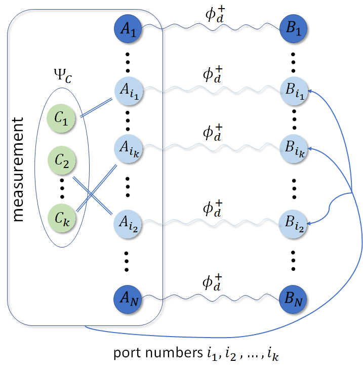
To perform teleportation of a state of kk multiparty systems one can: use the PBT with port dimension large enough, apply the PBT several times (sequential PBT), divide total number of ports into smaller packages and send every particle via such subsystem (packaged PBT), or finally apply multi-port based teleportation (MPBT) suggested in [28]. In particular, one could also run the recycling protocol for PBT suggested in [28], however due to recent results derived in [31] the efficiency of such scheme is an open problem. In the first case, increasing dimensionality of the port significantly reduces the entanglement fidelity [15, 29, 19, 18], requiring increasing the number of used ports to compensate it [9]. In sequential PBT and recycling protocol, we have to resign from single-shot scenario and after each round one needs to store the transmitted state, or we have to use distorted resource state, affecting the performance. In MPBT we allow to teleport a quantum multiparty state in one go, where each subsystem of the teleported multiparty system ends up in one of Bob’s ports, pointed by Alice’s message (see Fig. 2). The protocol thus enjoys quite a mild correction: Bob has to permute ports according to Alice’s message.

The main purpose of this paper is to evaluate and compare the transmission capability of PBT and MPBT schemes. More precisely, we consider teleportation of Nα\sim N^{\alpha} qubits (or more generally qudits) through NN ports, where NN grows to infinity, and analyse the quality of transmission, i.e. we ask about fidelity or probability of success. Note, in contrast with the traditional approach to channel capacity, where the central quantity is the asymptotic rate k/Nk/N, here the main objective becomes to identify asymptotic exponents α\alpha for which the transmission is possible, since the mentioned rate vanishes for port based teleportation.

In any variant of either of PBT and MPBT we obtain critical-like behaviour of the quality of transmission. We identify the critical values αcr\alpha_{\rm cr} of exponents α\alpha for several variants, both for exact asymptotic values of a figure of merit and their lower bounds. Whenever the value of α\alpha is below the critical value αcr\alpha_{\rm cr} the values of fidelity (or probability of success, depending on the scheme) describing transmission are 1, and 0 otherwise.

We obtain qualitative difference between deterministic scheme and probabilistic one. Namely, in the deterministic scheme, even the optimal PBT scheme is outperformed by non-optimal MPBT (i.e. one based on shared maximally entangled pairs). In particular, we argue that in non-optimal deterministic MPBT, one can teleport a much larger amount of quantum information, i.e. with αcr=1\alpha_{\rm cr}=1, in comparison to optimal port-based teleportation, where αcr=2/3\alpha_{\rm cr}=2/3, and one can teleport faithfully only up to o(N2/3)o(N^{2/3}) qubits.

Unlike in deterministic variant in probabilistic non-optimal MPBT the scaling is the same as for probabilistic optimal PBT, allowing for teleportation o(Nα)o(N^{\alpha}) qubits with αcr=1/2\alpha_{\rm cr}=1/2. However, considering an optimal version of probabilistic MPBT, one can transmit o(Nα)o(N^{\alpha}) with a critical exponent equal to 1, clearly outperforming PBT variants.

To achieve our results, we first provide a lower bound on fidelity in deterministic non-optimal MPBT based on the state discrimination problem. The new bound is effectively computable and depends only on global parameters like the number of ports, their dimension, and the number of teleported particles. The first bound of such kind has been discussed in [28] in not fully rigorous way, suffering from some flaws discussed later in this paper. In the qubit case, starting from group-theoretical results for exact values of entanglement fidelity and probability of success in non-optimal MPBT, presented in companion paper [30], we deliver exact and effectively computable expressions for these quantities in qubit case, phrased in appealing form of spin angular momentum. Next, result regarding asymptotic behaviour of non-optimal probabilistic case, have been obtained by combining advanced tools from statistical analysis, in particular non-straightforwardly the celebrated Berry-Essen theorem [6, 10] with direct estimates of binomial expressions by their Gaussian approximations. For optimal probabilistic MPBT we use for our analysis the exact formula for probability of success in such optimal MPBT derived in [20]. In the Table 1 we summarise the already mentioned variations of the architecture of PBT protocols, which are studied in this paper and are presented in more detail in the following sections.

Acronym Name Description Reference
(O)PBT(O)PBT (Optimal) port-based teleportation Teleportation of one qudit using NN entangled pairs, possibly with optimization over states and POVMs employed (optimal protocol) qbit case: [14, 15], qdit case:[29, 19]
(O)MPBT(O)MPBT (Optimal) multi port-based teleportation The teleportation of kk qudits in one go using NN entangled-pairs, includes the correction procedure in the last step, namely the permutation of the ports, see Fig. 2 this paper; companion papers [30, 20]
Pack. (O)PBT Packaged (optimal) port-based teleportation Teleportation of kk qdits by using kk (O)PBT schemes consisting of N/kN/k entangled-pairs, see Fig. 3 [28]
Table 1: Summary of different variations of Port Based Teleportation protocols discussed in this work. In each of them both deterministic and probabilistic scheme can be realised by choosing the appropriate measurement.

2 The Multi-port-based Teleportation

In order to transmit kk-system state ΨC=ΨC1C2Ck\Psi_{C}=\Psi_{C_{1}C_{2}\dots C_{k}} (see Fig. 2) Alice applies a global measurement Π𝐢AC\Pi_{\mathbf{i}}^{AC}, where A=A1ANA=A_{1}\dots A_{N}, on her halves of state ΦAB+=j=1N|ϕd+ϕd+|AjBj\Phi_{AB}^{+}=\bigotimes_{j=1}^{N}|\phi^{+}_{d}\rangle\langle\phi^{+}_{d}|_{A_{j}B_{j}} and the state to be teleported. As an output she receives a tuple of indices 𝐢={i1,i2,,ik}\mathbf{i}=\{i_{1},i_{2},\ldots,i_{k}\} and sends it to Bob through a classical channel. We denote the set of all outputs 𝐢\mathbf{i} by \mathcal{I}. Note that the number of outputs k!(Nk)k!\binom{N}{k} grows polynomially in NN at fixed kk. The meaning of indices (i1,,ik)(i_{1},\ldots,i_{k}) is that they point the ports on the receiver’s side on which the teleported systems appear, i.e. the first system arrives at port i1i_{1}, the second at i2i_{2} and so on. Bob recovers the initial form of the teleported state by suitably permuting his systems.
Refer to caption
Figure 2: In MPBT two parties share NN copies of the maximally entangled state (port) ϕd+=|ϕd+ϕd+|\phi_{d}^{+}=|\phi^{+}_{d}\rangle\langle\phi^{+}_{d}|, where |ϕd+=(1/d)i|ii|\phi^{+}_{d}\rangle=(1/\sqrt{d})\sum_{i}|ii\rangle. Alice to transmit a multipartite state θC\theta_{C} of kk systems performs a global measurement (POVM) on the state ΨC\Psi_{C} and her halves of the states ϕd+\phi^{+}_{d}. As an output she gets a string 𝐢={i1,i2,,ik}\mathbf{i}=\{i_{1},i_{2},\ldots,i_{k}\} indicating ports on the Bob’s side where the states arrive. To recover the state Bob has to pick up pointed ports in the right order, which is equivalent to permuting the ports according to message 𝐢\mathbf{i}. Similarly as it is for PBT here Alice can also jointly optimise over shared states and measurements getting optimal MPBT protocol.

The resulting action of the teleportation channel 𝒩\mathcal{N} is of the form

𝒩(ΨC)=𝐢TrAB¯𝐢C[Π𝐢AC(ΦAB+ΨC)Π𝐢AC]\displaystyle\mathcal{N}\left(\Psi_{C}\right)=\sum_{\mathbf{i}\in\mathcal{I}}\operatorname{Tr}_{A\bar{B}_{\mathbf{i}}C}\left[\sqrt{\Pi_{\mathbf{i}}^{AC}}\left(\Phi_{AB}^{+}\otimes\Psi_{C}\right)\sqrt{\Pi_{\mathbf{i}}^{AC}}^{\dagger}\right]
=𝐢TrAC[Π𝐢AC(σ𝐢ABΨC)],\displaystyle=\sum_{\mathbf{i}\in\mathcal{I}}\operatorname{Tr}_{AC}\left[\Pi_{\mathbf{i}}^{AC}\left(\sigma_{\mathbf{i}}^{AB}\otimes\Psi_{C}\right)\right], (1)

where the bar in B¯𝐢\bar{B}_{\mathbf{i}} denotes discarded subsystems except those on positions i1,i2,,iki_{1},i_{2},\ldots,i_{k}. The states σ𝐢AB\sigma_{\mathbf{i}}^{AB} or shortly σ𝐢\sigma_{\mathbf{i}} for 𝐢\mathbf{i}\in\mathcal{I}, called later the signals, are given as

σ𝐢ABTrB¯𝐢ΦAB+=1dNk𝟏A¯𝐢ϕA𝐢B𝐢+,\begin{split}\sigma_{\mathbf{i}}^{AB}&\equiv\operatorname{Tr}_{\bar{B}_{\mathbf{i}}}\Phi_{AB}^{+}=\frac{1}{d^{N-k}}\mathbf{1}_{\bar{A}_{\mathbf{i}}}\otimes\phi^{+}_{A_{\mathbf{i}}B_{\mathbf{i}}},\end{split} (2)

where ϕA𝐢B𝐢+=|ϕd+ϕd+|A𝐢B𝐢\phi^{+}_{A_{\mathbf{i}}B_{\mathbf{i}}}=|\phi_{d}^{+}\rangle\langle\phi_{d}^{+}|_{A_{\mathbf{i}}B_{\mathbf{i}}}. To examine the efficiency we compute the entanglement fidelity which reports how well parties can transmit quantum correlations by sending kk halves of maximally entangled states Φ+CD=ϕC1D1+ϕC2D2+ϕCkDk+\Phi^{+}_{CD}=\phi_{C_{1}D_{1}}^{+}\otimes\phi_{C_{2}D_{2}}^{+}\otimes\cdots\otimes\phi_{C_{k}D_{k}}^{+}:

F=Tr[ΦBD+(𝒩𝟏D)(ΦCD+)]=1d2k𝐢Tr[Π𝐢ABσ𝐢AB].\begin{split}F&=\operatorname{Tr}\left[\Phi^{+}_{BD}(\mathcal{N}\otimes\mathbf{1}_{D})\left(\Phi^{+}_{CD}\right)\right]=\frac{1}{d^{2k}}\sum_{\mathbf{i}\in\mathcal{I}}\operatorname{Tr}\left[\Pi_{\mathbf{i}}^{AB}\sigma_{\mathbf{i}}^{AB}\right].\end{split} (3)

In the probabilistic scheme the teleportation channel looks exactly as in (2), but with different form of measurements. The channel is now trace non-preserving, since there is a POVM, denoted as Π𝟎AB\Pi_{\mathbf{0}^{AB}}, corresponding to the failure of the whole process. The average probability of success reads [14, 30]:

psucc=1dN+k𝐢Tr[Π𝐢AB].p_{succ}=\frac{1}{d^{N+k}}\sum_{\mathbf{i}\in\mathcal{I}}\operatorname{Tr}\left[\Pi_{\mathbf{i}}^{AB}\right]. (4)

The goal here is to find the set of optimal measurements, maximising the probability of success. This is done in [30] by exploiting symmetries exhibit in the problem and methods from semidefinite programming. Our considerations look similar to the original PBT scheme, but incorporating kk particles into the teleportation process makes it structurally entirely different, see [30]. The structure of the signals σ𝐢AB\sigma_{\mathbf{i}}^{AB} and the suitable measurements Π𝐢AB\Pi_{\mathbf{i}}^{AB}, makes the problem of evaluating FF and psuccp_{succ} very hard and technical. Therefore, in the next section, we present an effectively computable lower bound on the entanglement fidelity.

3 Fidelity bound from the state discrimination task

Evaluation of fidelity in the standard PBT was a formidable task, requiring machinery of representation theory of SU(2)NSU(2)^{\otimes N} for qubits, and much more advanced representation theoretic tools for d>2d>2. The resulting formulas are usually not very transparent, expressed in terms of complicated sums of representation theory parameters, for which no explicit expressions are known beyond qubits.

The first attempt to derive the efficiency of deterministic MPBT has been presented in [28]. The combinatorial argumentation used by the authors was incorrect, neglecting deeper complexity of the problem. However, one can save part of argumentation and show that the bound given in [28] is indeed a legitimate lower bound for fidelity, see discussion after example 14 in Appendix B. Here, we go further and give a simple and stronger lower bound for fidelity of the protocol. The starting point is the idea presented [14, 15], exploited in [4, 28], of providing lower bound for the standard PBT protocol by relating fidelity of teleportation to probability of success in state discrimination. Let us emphasize, that generalizing this approach to the multiport scheme case requires solving a complex combinatorial problem, contained in Lemma 1.

The relation between the entanglement fidelity and the averaged probability pdistp_{dist} of distinguishing the signals σ𝐢\sigma_{\mathbf{i}} with equal prior probability 1/(k!(Nk))1/(k!\binom{N}{k}) for arbitrary measurements Π𝐢\Pi_{\mathbf{i}} is given by (see [4]):

F=k!(Nk)d2kpdist,pdist=1k!(Nk)𝐢Tr(Π𝐢σ𝐢).F=\frac{k!\binom{N}{k}}{d^{2k}}p_{dist},\qquad p_{dist}=\frac{1}{k!\binom{N}{k}}\sum_{\mathbf{i}\in\mathcal{I}}\operatorname{Tr}(\Pi_{\mathbf{i}}\sigma_{\mathbf{i}}). (5)

Now, our goal is to provide effectively computable lower bound on pdistp_{dist}, which gives us the lower bound on FF of our protocol. Since we are interested in any feasible lower bound, for any k1k\geq 1, in (5) we take square-root measurements (SRM) of the form:

Π𝐢=ρ1/2σ𝐢ρ1/2withρ=𝐢σi.\Pi_{\mathbf{i}}=\rho^{-1/2}\sigma_{\mathbf{i}}\rho^{-1/2}\quad\text{with}\quad\rho=\sum_{\mathbf{i}\in\mathcal{I}}\sigma_{i}. (6)

The support of square-root measurements is always restricted to the support of the signals σ𝐢\sigma_{\mathbf{i}} [14, 30] making explicit calculations difficult. However, by formulating the generalisation of the statement of Lemma A.3 from [4] (see also Appendix B for details), we get a general lower bound on pdistp_{dist}:

pdist1dNkTrρ¯2,p_{dist}\geq\frac{1}{d^{N-k}\operatorname{Tr}\overline{\rho}^{2}}, (7)

where ρ¯\overline{\rho} is a normalised version of the operator ρ\rho from (6). To use (7) one has to evaluate Trρ¯2\operatorname{Tr}\overline{\rho}^{2}. The result (Appendix B) is the following:

Lemma 1.

For the operator ρ¯=ρ/Trρ\overline{\rho}=\rho/\operatorname{Tr}\rho, we have

Tr(ρ¯2)=dNk(Nk)1(d2+N1k).\operatorname{Tr}(\overline{\rho}^{2})=d^{-N-k}\binom{N}{k}^{-1}\binom{d^{2}+N-1}{k}. (8)

Now we are in position to provide our lower bound for teleportation fidelity.

Theorem 2.

The entanglement fidelity FF in MPBT deterministic scheme, with NN ports of dimension dd each, while teleporting kN/2k\leq\lfloor N/2\rfloor particles satisfies

F(Nk)(d2+N1k)1(1d21d2+Nk)k.\begin{split}F\geq\binom{N}{k}\binom{d^{2}+N-1}{k}^{-1}\geq\left(1-\frac{d^{2}-1}{d^{2}+N-k}\right)^{k}.\end{split} (9)

For fixed kk the fidelity scales at least as 1O(1/N)1-O(1/N) and for NN\to\infty the fidelity goes to 11.

The first bound in (9) follows from Lemma 1 and expression (5). The proof of second estimate, being technical, we delegate to Appendix B. The last sentence of the Theorem is obtained by applying the Bernoulli inequality (1x)k1kx(1-x)^{k}\geq 1-kx (valid for x<1x<1) to the second bound. In particular, for qubits it reads:

F13k4+Nk.F\geq 1-\frac{3k}{4+N-k}. (10)

For k=1k=1, the bound in (9) reduces to the bound for the standard non-optimal PBT [4], namely F1d21d2+N1F\geq 1-\frac{d^{2}-1}{d^{2}+N-1}.

Now we compare performance of MPBT with the port based teleportation protocols by considering packaged PBT [28]. We shall compare MPBT protocols only with the mentioned versions of PBT, since the versions with large port dimension dkd^{k} become ineffective very fast [9] and fidelity drops substantially. For our considerations we use both the original, i.e. non-optimal PBT protocol (Figure 1), where Alice and Bob share NN maximally entangled states, as well as the optimized version of PBT scheme (OPBT), where Alice optimises over shared state and measurements. Let us emphasize that in our scheme we do not perform any optimisation as it is done in OPBT case and, moreover, we compare with the lower bound in Theorem 2.

Let us denote by F(N,k)F(N,k) the fidelity of teleportation, regardless of the scheme, of kk qubit systems through NN ports.

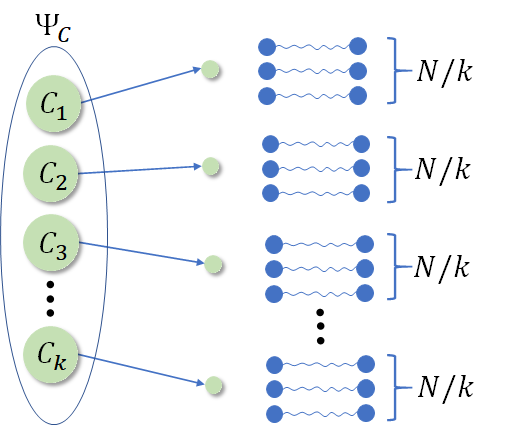
Packaged PBT In this version Alice to transmit kk-system state to Bob has to divide all the ports in her possession in N/kN/k packages (see Figure 3). Then she runs independently kk separate PBT protocols with N/kN/k ports each. The total fidelity Fpack(N,k)F_{pack}(N,k) in the packaged version of PBT equals

Fpack(N,k):=F(N/k,1)k.F_{pack}(N,k):=F(N/k,1)^{k}. (11)

Please notice that optimal MPBT protocol is at least good as packaged PBT, since optimisation over the resource state includes all packaged schemes. Here however, we compare packaged versions of PBT with lower bound from Theorem 2, so it could happen in principle that the lower bound performs worse than packaged PBT.

In paper [28] it was shown that in case of qubits the quantity Fpack(N,k)F_{pack}(N,k) can be bounded from below as

Fpack(N,k)=(13k4N)k13k24N.F_{pack}(N,k)=\left(1-\frac{3k}{4N}\right)^{k}\geq 1-\frac{3k^{2}}{4N}. (12)

However, it is easy to check that bound given through Theorem 2 outperforms bound (12) for k4k\geq 4. This motivates us to compare bound (9) with exact values of the packaged PBT given by (11).
Refer to caption
Figure 3: The packaged protocol for PBT. Alice to send a kk-system state ΨC1C2Ck\Psi_{C_{1}C_{2}\ldots C_{k}} to Bob divides all the ports into N/kN/k packages, and performs kk independent PBT protocols with N/kN/k ports each.

We know from [15], that the fidelity for qubit optimal PBT is given by F=cos2(πN+2)F=\operatorname{cos}^{2}\left(\frac{\pi}{N+2}\right). Then in the packaged version entanglement fidelity reads

FpackOPBT(N,k)=cos2k(πN/k+2).F_{pack}^{OPBT}(N,k)=\operatorname{cos}^{2k}\left(\frac{\pi}{N/k+2}\right). (13)

In Figure 4 we present comparison of the first bound from (9), plotted for various kk versus the fidelity of the packaged OPBT (13).

In our comparisons we use only the lower bound for non-optimal MPBT from Theorem 2, getting regions for which we perform better. For the exact values we obviously perform even better. In Appendix C we present an explicit expression for the entanglement fidelity in the qubit case, using angular momentum representation, and we compare it with the second bound from Theorem 2.
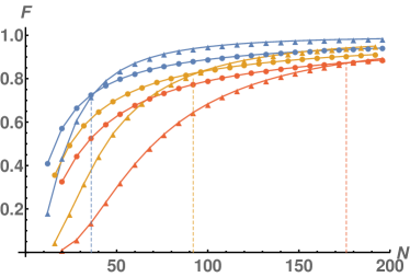
Figure 4: Comparison of the first bound from (9) from Theorem 2 (full circles, for k=4k=4 marked with Refer to caption, k=6k=6 Refer to caption, k=8k=8 Refer to caption) with exact values of the Pack. OPBT (13) (triangles, for fixed k=4k=4 Refer to caption, k=6k=6 Refer to caption, k=8k=8 Refer to caption). For each fixed k=4,6,8k=4,6,8 there exists NN for which the packaged version of OPBT outperforms the bound. We see, however, that for increasing number kk of teleported qubits, the region of supremacy of MPBT scheme increases quickly.

For fixed kk and small number of ports NN our first bound outperforms packaged OPBT from (11). However, for every fixed kk there is some point after which FpackOPBT(N,k)F_{pack}^{OPBT}(N,k) dominates over the first (stronger) bound given by (9). Nevertheless, as kk increase this point shifts more rapidly. This suggests, that changing kk adaptively with growing NN shows the real advantage of the new protocol over the preexisting ones. We examine it in Section 4.1.

4 Multiport versus standard PBT: large number of teleported qubits

4.1 Deterministic protocol

We now compare performance of the MPBT protocol with the packaged (O)PBT ones in the asymptotic regime, when we change the number of teleported particles adaptively. Namely, we shall assume that the number of teleported particles scales as k(N)=aNαk(N)=aN^{\alpha}.

For the case of MPBT we can formulate

Proposition 3.

When k/N0k/N\to 0, the fidelity approaches 11. Moreover, for k=aNk=\lfloor aN\rfloor where a<1a<1 we have limNFe(d21)a1a.\lim_{N\to\infty}F\geq\operatorname{e}^{-(d^{2}-1)\frac{a}{1-a}}.

When k=aNk=\lfloor aN\rfloor the statement of the Proposition follows directly from the calculation of the limit of the first bound given in (9). The case k=o(N)k=o(N) follows from applying Bernoulli inequality (1x)k1kx(1-x)^{k}\geq 1-kx (valid for x<1x<1) to the second bound in (9).

The relation between α\alpha and the asymptotic fidelity of PBT and OPBT protocols is as follows. For the non-optimal PBT protocol the fidelity fulfils F134N=1O(1/N)F\approx 1-\frac{3}{4N}=1-O(1/N) [15]. Thus, we can easily calculate limNFpackPBT(N,k)\lim_{N\rightarrow\infty}F^{PBT}_{pack}(N,k) for the non-optimal packaged PBT. It turns out that depending on whether α\alpha is greater, smaller or equal to particular value αcr\alpha_{cr} (which in this case equals 1/21/2) the asymptotic fidelity equals 0,10,1 or a fixed value FcrF_{cr}.

For FpackOPBT(N,k)F_{pack}^{OPBT}(N,k) we can apply exactly the same reasoning, since in that case F=cos2(πN+2)1π2/N2F=\operatorname{cos}^{2}\left(\frac{\pi}{N+2}\right)\approx 1-{\pi^{2}}/{N^{2}} [15].

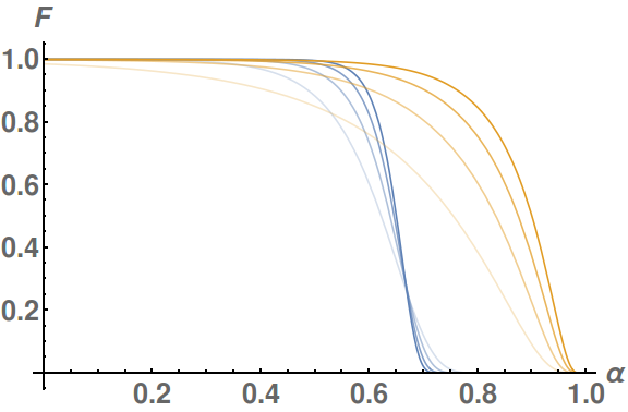
The results for all three schemes are presented in the Table 2 and the convergence for OPBT and MPBT protocols is depicted in the Figure 5.

F=0F=0 Fcr\qquad\qquad F_{\rm cr} F=1F=1
Pack.PBTPack.PBT α>1/2\alpha>1/2 αcr=1/2\alpha_{\rm cr}=1/2\,, Fcr=e3a2/4F_{\rm cr}=e^{-3a^{2}/4} α<1/2\alpha<1/2
Pack.OPBTPack.OPBT α>2/3\alpha>2/3 αcr=2/3\alpha_{\rm cr}=2/3\,, Fcr=eπ2a3F_{\rm cr}=e^{-\pi^{2}a^{3}} α<2/3\alpha<2/3
MPBTMPBT - αcr=1,\alpha_{\rm cr}=1,\ \ \ Fcre3a1aF_{\rm cr}\geq e^{-\frac{3a}{1-a}} α<1\alpha<1
Table 2: Comparison of the asymptotic behaviour of two variants of packaged PBT with MPBT in deterministic version, where k=aNαk=aN^{\alpha}. By "cr" we denote the critical values of parameter α\alpha for which asymptotic value of FF exhibits a jump.
Refer to caption
Figure 5: Asymptotic values of the lower bound on entanglement fidelity in MPBT (orange lines) compared to the fidelity of Pack. OPBT (blue lines), where k=aNα,a=1,α(0,1)k=aN^{\alpha},a=1,\;\alpha\in{(0,1)}, see Table 2. NN runs through 102,103,10410^{2},10^{3},10^{4} and 10510^{5} as the lines become thicker.

MPBT scheme offers qualitative improvement over the original scheme for teleporting multipartite states. Even in optimal scheme of standard PBT (i.e. one, with optimal POVMs and the resource state) the number of teleported qubits can only scale as N2/3N^{2/3}, while in the original scheme, (where the resource state is just NN EPR pairs) the scaling is N1/2N^{1/2}.

4.2 Probabilistic protocol

Here we shall compare MPBT versus packaged PBT scheme in probabilistic scenario, where the figure of merit is probability of success. Again we will assume that k=aNαk=aN^{\alpha}. We do not have here such simple explicit bounds as those given in Theorem 2. We shall therefore use exact formula derived in companion paper by means of representation theoretic tools [30]. Basing on this result, in Appendix C we present exact formula for the probability of success in qubit case expressed in terms of angular momentum parameters which reads:

psucc(N,k)=12N1N+1s=0(12)Nk2(2s+1)2(N+1Nk2s).p_{succ}(N,k)=\frac{1}{2^{N}}\frac{1}{N+1}\sum_{s=0(\frac{1}{2})}^{\frac{N-k}{2}}(2s+1)^{2}\binom{N+1}{\frac{N-k}{2}-s}. (14)
ps=0p_{s}=0 ps,cr\qquad\qquad p_{s,\rm cr} ps=1p_{s}=1
Pack.PBTPack.PBT α>1/3\alpha>1/3 αcr=1/3\alpha_{\rm cr}=1/3\,, ps,cr=eca3/2p_{s,\rm cr}=e^{-ca^{3/2}} α<1/3\alpha<1/3
Pack.OPBTPack.OPBT α>1/2\alpha>1/2 αcr=1/2,\alpha_{\rm cr}=1/2,\, ps,cr=e3a2p_{s,\rm cr}=e^{-3a^{2}} α<1/2\alpha<1/2
MPBTMPBT α>1/2\alpha>1/2 αcr=1/2,\alpha_{\rm cr}=1/2,\ eq. (15) α<1/2\alpha<1/2
OMPBTOMPBT - αcr=1,\alpha_{\rm cr}=1,\ \ ps,cr=(1+a)3p_{s,\rm cr}=(1+a)^{3} α<1\alpha<1
Table 3: Table collects the comparison of the asymptotic behaviour of probability of success psp_{s} of all variants of packaged PBT with MPBT in probabilistic version when k=aNαk=aN^{\alpha}. Here c=8/πc=\sqrt{8/\pi}. By "cr" we denote the critical values of parameter α\alpha for which asymptotic value of psp_{s} exhibits a jump.

Setting k=aNk=a\sqrt{N} we can examine the dependence of (14) on aa. We can observe, that when a0a\to 0 then psucc1p_{succ}\to 1. The latter is given (15), proven in Appendix D with the means of Central Limit type theorem, although in not completely straightforward way.

limNpsucc={20x212πe(x+a)22dx,k=aN,a>01,k=o(N)\lim_{N\to\infty}p_{succ}=\begin{cases}2\int_{0}^{\infty}x^{2}\frac{1}{\sqrt{2\pi}}\operatorname{e}^{-\frac{(x+a)^{2}}{2}}dx,\;&k=a\sqrt{N},a>0\\ 1,\quad&k=o(\sqrt{N})\par\end{cases} (15)

For PBT, in the case of original (i.e. nonoptimized) scheme [15] we have psucc1c/Np_{succ}\approx 1-c/\sqrt{N}, where c=8πc=\sqrt{\frac{8}{\pi}}, and psucc=13/(3+N)13/Np_{succ}=1-3/{(3+N)}\approx 1-3/{N} in the case of OPBT [15]. We may then apply the same reasoning as in the deterministic case. Considering (14) we can see that

limNpsuccMPBT=1 for α<1/2.\lim_{N\rightarrow\infty}p_{succ}^{MPBT}=1\text{ for }\alpha<1/2. (16)

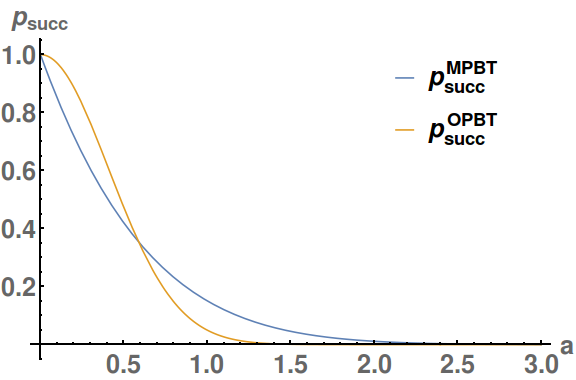
We can thus see that, unlike the deterministic protocol, the regions of asymptotic behaviour of psuccp_{succ} are separated by the same critical value αcr=1/2\alpha_{cr}=1/2 for packaged OPBT and MPBT probablistic protocols. Plotting psuccMPBTp_{succ}^{MPBT} and psuccOPBTp_{succ}^{OPBT} as a function of aa in this borderline case, i.e. when α=αcr=1/2\alpha=\alpha_{cr}=1/2 (see Figure 6), we observe the new protocol outperforms the previous one in the regime of large aa.

Refer to caption
Figure 6: The limiting probability of success in the probabilistic schemes: Pack. OPBT(orange line) and MPBT (blue line) plotted as a function of aa when k=aNk=a\sqrt{N}, i.e. α=1/2\alpha=1/2, see Table 3.

However, one can refer to recent result concerning optimal MPBT [20], where remarkably simple expression for probability of success is evaluated:

psuccOMPBT=m=2d2(1kN1+m).p_{succ}^{OMPBT}=\prod\limits_{m=2}^{d^{2}}\left(1-\frac{k}{N-1+m}\right). (17)

This for k=o(N)k=o(N) leads to limNpsuccOMPBT=1\lim_{N\rightarrow\infty}p_{succ}^{OMPBT}=1. We have for d=2d=2

limNpsuccOMPBT={(1a)3,k=aN1,k=o(N)\lim_{N\rightarrow\infty}p_{succ}^{OMPBT}=\begin{cases}(1-a)^{3},&k=aN\\ 1,&k=o(N)\end{cases} (18)

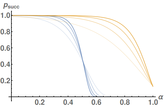
which outperforms the optimal PBT. This for k=o(N)k=o(N) leads to limNpsuccOMPBT=1\lim_{N\rightarrow\infty}p_{succ}^{OMPBT}=1. Moreover, for d=2d=2 and k=aNk=aN, that limNpsuccOMPBT=(1a)3\lim_{N\rightarrow\infty}p_{succ}^{OMPBT}=(1-a)^{3}, which outperforms the optimal packaged PBT. We present the comparison of scaling of the packaged OPBT and OMPBT protocols in the Table 3 and Figure 7.
Refer to caption
Figure 7: Probability of success, compared for Pack. OPBT (blue lines), and OMPBT (orange lines) protocols, where k=aNα,a=12k=aN^{\alpha},a=\frac{1}{2}, see Table 3. NN runs through 102,103,10410^{2},10^{3},10^{4} and 10510^{5} as the lines become thicker.

Finally, for a finite number of ports NN we have precise lower and upper bound for psuccp_{succ} in our protocol, which are presented in the Appendix D.

5 Conclusions and Discussions

We have addressed the problem of teleporting a large amount of quantum information. In particular we analyse quantum multi-port teleportation protocol performing transmission of several quantum systems in one round. By examining improved lower bound on its performance, measured in the entanglement fidelity, we show that the protocol outperforms introduced earlier PBT protocols. The bound has been obtained by considering the teleportation process in our protocol as a state discrimination task and it depends only on global parameters like the number of ports, their dimension, and the number of teleported particles. In particular, we derived closed expressions for the entanglement fidelity and the probability of success in the described scheme for qubits in the picture of the angular momentum and using Gaussian approximation.

Further, we have shown that in general the number of systems to be teleported can be changed dynamically by the sender with the growing number of ports, still ensuring high efficiency in deterministic and probabilistic scheme. Even in the optimal PBT scheme, in deterministic case, fidelity can approach 11 for teleporting of up to N2/3N^{2/3} particles, for our MPBT NαN^{\alpha} particles can be teleported, if only α<1\alpha<1. In probabilistic case, although the rates are equal and the teleportation achieving asymptotically unit probability of success is possible for number of teleported particles of the order Nα,α<1/2N^{\alpha},\alpha<1/2, both in MPBT and OPBT, we present result concerning optimal MPBT, which outperforms previous protocols [20].

We have thus showed that analysed protocol, while still requiring quite mild correction on Bob’s site (just permuting his systems), exhibits qualitatively better "capacity" of transmission. Our results pave a novel way in teleportation and quantum communication in general. So far in quantum communication, while sending quantum information, one was interested in linear rate, i.e. the number of sent qubits per number of channel (or entangled pair) uses. On the other hand in quantum computing, it is very important to have teleportation with less correction on receiver’s side. The port-based teleportation is protocol with virtually no correction. Here, we consider for the first time the issue of the amount of quantum information sent via such teleportation protocols. Our work implies, that within the realm of weakened correction - the proper notion of communication efficiency is determined by asymptotic exponents in first place.

Still, there are a few open questions. First, except probabilistic OMPBT, we do not have exact asymptotic expressions for d>2d>2. However, application of central limit theorem or adaptation techniques from [9] theorem should lead to the solution. In the case of deterministic OMPBT the problem of getting the asymptotic behaviour is more complex, since we do not have a closed formula for the fidelity. The fidelity there is given in terms of maximal eigenvalue of teleportation matrix [19, 30], for which we do not have an analytical formula yet, even for k=1k=1. Finally, we leave the rigorous analysis of the recycling protocol introduced in [28] and its comparsion with our results for further project.

Acknowledgements MS, MM are supported through grant Sonatina 2, UMO-2018/28/C/ST2/00004 from the Polish National Science Centre. Moreover, MH and MM thank the Foundation for Polish Science through IRAP project co-financed by the EU within the Smart Growth Operational Programme (contract no. 2018/MAB/5). MH also acknowledges support from the National Science Centre, Poland, through grant OPUS 9, 2015/17/B/ST2/01945. MM and PK would like to thank ICTQT Centre (University of Gdańsk) for hospitality where part of this work has been done.

Appendix A Symmetries in Multi-port teleportation scheme

Before we present argumentation leading us to the proof of Lemma 1 from the main text, we introduce here concepts of permutation operator and its partial transposition. Most of the formalism presented here can be also find in [30, 17]. Let us consider a representation VV of the permutation group S(n)S(n) in the space (d)n\mathcal{H\equiv(\mathbb{C}}^{d})^{\otimes n}, defined in the following way

πS(n)V(π).|ei1|ei2|ein:=|eiπ1(1)|eiπ1(2)|eiπ1(n),\forall\pi\in S(n)\qquad V(\pi).|e_{i_{1}}\rangle\otimes|e_{i_{2}}\rangle\otimes\cdots\otimes|e_{i_{n}}\rangle:=|e_{i_{\pi^{-1}(1)}}\rangle\otimes|e_{i_{\pi^{-1}(2)}}\rangle\otimes\cdots\otimes|e_{i_{\pi^{-1}(n)}}\rangle, (19)

where the set {|ei}i=1d\{|e_{i}\rangle\}_{i=1}^{d} is an orthonormal basis of the space d\mathcal{\mathbb{C}}^{d}, and dd stands for the dimension. We drop here the lower index in every ii, since it labels only position of the basis in tensor product (d)n(\mathbb{C}^{d})^{\otimes n}. This representation is in fact a unitary matrix representation, since it is given with respect to prescribed basis {|ei}i=1d\{|e_{i}\rangle\}_{i=1}^{d} in the space d\mathcal{\mathbb{C}}^{d}, and for every πS(n)\pi\in S(n) the corresponding matrix representation V(π)V(\pi) is called a permutation operator. The representation VV of S(n)S(n) extends in a natural way to the representation of the group algebra [S(n)]\mathbb{C}[S(n)] and in this way we get the algebra of permutation operators

𝒜n(d)span{V(π):πS(n)}.\mathcal{A}_{n}(d)\equiv\operatorname{span}_{\mathbb{C}}\{V(\pi):\pi\in S(n)\}. (20)

Having the above definition of the algebra 𝒜n(d)\mathcal{A}_{n}(d), we can introduce a new complex algebra - algebra of the partially transposed permutation operators:

𝒜n(k)(d)span{V(k)(π):πS(n)},\mathcal{A}_{n}^{(k)}(d)\equiv\operatorname{span}_{\mathbb{C}}\{V^{(k)}(\pi):\pi\in S(n)\}, (21)

where the symbol (k)(k) denotes partial transpose operation with respect to last kk systems in the space (d)n.\mathcal{(\mathbb{C}}^{d})^{\otimes n}. Now, we show that the operator ρ\rho defined in expression (6) from the main text is an element of the algebra 𝒜n(k)(d)\mathcal{A}_{n}^{(k)}(d). Let us denote by n=N+kn=N+k the number of all systems involved in the teleportation process on Alice’s (Bob’s) side and introduce the following mapping of indices

𝐢B𝐢B=Bnk+1Bnk+2Bnk.\forall\ \mathbf{i}\in\mathcal{I}\quad B_{\mathbf{i}}\mapsto B=\underbrace{B_{n-k+1}B_{n-k+2}\cdots B_{n}}_{k}. (22)

Having that we can work with the equivalent form of the operator ρ\rho, which is given through the following expression

ρ=𝐢σi=1dNk𝐢𝟏A¯𝐢PA𝐢B+,\rho=\sum_{\mathbf{i}\in\mathcal{I}}\sigma_{i}=\frac{1}{d^{N-k}}\sum_{\mathbf{i}\in\mathcal{I}}\mathbf{1}_{\bar{A}_{\mathbf{i}}}\otimes P^{+}_{A_{\mathbf{i}}B}, (23)

where for a given index 𝐢={i1,i2,,ik}\mathbf{i}=\{i_{1},i_{2},\ldots,i_{k}\} the operator 𝟏A¯𝐢PA𝐢B+\mathbf{1}_{\bar{A}_{\mathbf{i}}}\otimes P^{+}_{A_{\mathbf{i}}B} is of the following form

σ𝐢=𝟏A¯𝐢P+A𝐢B=𝟏A¯𝐢P+i1,nk+1P+i2,nk+2P+ik,n=1dN𝟏A¯𝐢Vtnk+1[(i1,nk+1)]Vtnk+2[(i2,nk+2)]Vtn[(ik,n)].\begin{split}\sigma_{\mathbf{i}}&=\mathbf{1}_{\bar{A}_{\mathbf{i}}}\otimes P^{+}_{A_{\mathbf{i}}B}=\mathbf{1}_{\bar{A}_{\mathbf{i}}}\otimes P^{+}_{i_{1},n-k+1}\otimes P^{+}_{i_{2},n-k+2}\otimes\cdots\otimes P^{+}_{i_{k},n}\\ &=\frac{1}{d^{N}}\mathbf{1}_{\bar{A}_{\mathbf{i}}}\otimes V^{t_{n-k+1}}[(i_{1},n-k+1)]\otimes V^{t_{n-k+2}}[(i_{2},n-k+2)]\otimes\cdots\otimes V^{t_{n}}[(i_{k},n)].\end{split} (24)

By tnk+1,tnk+2,,tnt_{n-k+1},t_{n-k+2},\ldots,t_{n} we denote transposition with respect to systems on positions nk+1,nk+2,,nn-k+1,n-k+2,\ldots,n respectively. Next, we have to rewrite ρ\rho in more convenient form for our further considerations. First, we observe that we can distinguish an index 𝐢0={nk,nk1,,n2k+1}\mathbf{i}_{0}=\{n-k,n-k-1,\ldots,n-2k+1\}, for which the corresponding signal is called canonical:

σ𝐢0=1dN𝟏A¯𝐢0Vtnk+1[(nk,nk+1)]Vtnk+2[(nk1,nk+2)]Vtn[(n2k+1,n)]=1dN(𝟏A¯𝐢0V[(nk,nk+1)]V[(nk1,nk+2)]V[(n2k+1,n)])tnk+1tnk+2tn=1dNV(k),\begin{split}\sigma_{\mathbf{i}_{0}}&=\frac{1}{d^{N}}\mathbf{1}_{\bar{A}_{\mathbf{i}_{0}}}\otimes V^{t_{n-k+1}}[(n-k,n-k+1)]\otimes V^{t_{n-k+2}}[(n-k-1,n-k+2)]\otimes\cdots\otimes V^{t_{n}}[(n-2k+1,n)]\\ &=\frac{1}{d^{N}}\left(\mathbf{1}_{\bar{A}_{\mathbf{i}_{0}}}\otimes V[(n-k,n-k+1)]\otimes V[(n-k-1,n-k+2)]\otimes\cdots\otimes V[(n-2k+1,n)]\right)^{t_{n-k+1}t_{n-k+2}\cdots t_{n}}\\ &=\frac{1}{d^{N}}V^{(k)},\end{split} (25)

by VV we denote the total permutation operator in the bracket with this specific composition of permutations, including the identity operator. Having the definition of σ𝐢0\sigma_{\mathbf{i}_{0}}, let us observe that any other signal can be obtained from it by acting of V(τ)V(\tau), where τ\tau is permutation from the coset 𝒮n,k=S(nk)/S(n2k)\mathcal{S}_{n,k}=S(n-k)/S(n-2k), so

ρ=1dNτ𝒮n,kV(τ)V(k)V(τ).\rho=\frac{1}{d^{N}}\sum_{\tau\in\mathcal{S}_{n,k}}V(\tau)V^{(k)}V^{\dagger}(\tau). (26)

This clearly shows that the operator ρ\rho, as well as every operator σ𝐢\sigma_{\mathbf{i}} belongs to the algebra 𝒜n(k)(d)\mathcal{A}_{n}^{(k)}(d) defined in (21). The cardinality of 𝒮n,k\mathcal{S}_{n,k} gives us number of all possible signals k!(Nk)k!\binom{N}{k}. Since all the operators V(τ)V(\tau) are invariant with respect to the composition of partial transpositions (k)(k), we can rewrite ρ\rho from (26) as in the following definition:

Definition 4.

For NN ports the operator ρ\rho from expression (26) can be re-written in the following form:

ρa1,a2,,ak=1nkV(k)[(ak,nk+1)(ak1,nk+2).(a1,n)],\rho\equiv\sum_{a_{1},a_{2},\ldots,a_{k}=1}^{n-k}V^{(k)}[(a_{k},n-k+1)(a_{k-1},n-k+2).\cdots(a_{1},n)], (27)

where all numbers a1,a2,,aka_{1},a_{2},\ldots,a_{k} are different and kN2k\leq\lfloor\frac{N}{2}\rfloor. For compactness of the further calculations we drop here the normalisation constant 1/dN1/d^{N} in form of every signal σ𝐢\sigma_{\mathbf{i}}.

Appendix B Proof of Lemma 1 and Theorem 1 from the main text

Having discussion on symmetries in multi-port based teleportation protocols we are in position to compute the lower bound on the entanglement fidelity FF. As it was pointed in the main text, and in [14, 4], the entanglement fidelity FF can be connected with probability of success of the state discrimination pdistp_{dist} of the ensemble \mathcal{E}:

={1k!(Nk),σ𝐢},\mathcal{E}=\left\{\frac{1}{k!\binom{N}{k}},\sigma_{\mathbf{i}}\right\}, (28)

where σ𝐢\sigma_{\mathbf{i}} are the signal states described in Section A. It can be shown that FF and pdistp_{dist} are related to each other by the following relation

F=k!(Nk)d2kpdist,pdist=1k!(Nk)𝐢Tr(Π𝐢σ𝐢)1k!(Nk)rTrρ¯2,F=\frac{k!\binom{N}{k}}{d^{2k}}p_{dist},\qquad p_{dist}=\frac{1}{k!\binom{N}{k}}\sum_{\mathbf{i}\in\mathcal{I}}\operatorname{Tr}(\Pi_{\mathbf{i}}\sigma_{\mathbf{i}})\geq\frac{1}{k!\binom{N}{k}r\operatorname{Tr}\overline{\rho}^{2}}, (29)

where r=(1/(k!(Nk)))𝐢rank(σ𝐢)=dNkr=(1/(k!\binom{N}{k}))\sum_{\mathbf{i}\in\mathcal{I}}\operatorname{rank}(\sigma_{\mathbf{i}})=d^{N-k}, and the lower bound on pdistp_{dist} is a simple generalisation of Lemma A.3 from [4]. This means that FF is bounded from the below as

F1dN+kTr(ρ¯2),F\geq\frac{1}{d^{N+k}\operatorname{Tr}(\overline{\rho}^{2})}, (30)

where the operator ρ¯\overline{\rho} is normalised version (Trρ¯=1\operatorname{Tr}\overline{\rho}=1) of the operator ρ\rho from Definition 4:

ρ¯=ρTr(ρ)=1dNk!(Nk)ρ,\overline{\rho}=\frac{\rho}{\operatorname{Tr}(\rho)}=\frac{1}{d^{N}k!\binom{N}{k}}\rho, (31)

since we can observe that for operator ρ\rho from Definition 4 the following holds

Tr(ρ)=dnk(nk)(nk1)(n2k+1)=dNN(N1)(Nk+1)=dNk!(Nk)=dNN!(Nk)!,\begin{split}\operatorname{Tr}(\rho)&=d^{n-k}(n-k)(n-k-1)\cdot\ldots\cdot(n-2k+1)=d^{N}N(N-1)\cdot\ldots\cdot(N-k+1)=d^{N}k!\binom{N}{k}\\ &=d^{N}\frac{N!}{(N-k)!},\end{split} (32)

where N=nkN=n-k denotes number of ports. It means that normalised operator ρ¯\overline{\rho} can be written finally as

ρ¯=ρTr(ρ)=1dNN!(Nk)!ρ.\overline{\rho}=\frac{\rho}{\operatorname{Tr}(\rho)}=\frac{1}{d^{N}\frac{N!}{(N-k)!}}\rho. (33)

Later on we use form of ρ¯\overline{\rho} from expression (33).

The above considerations show that to compute the right-hand side of (30) the crucial is evaluation of Tr(ρ2)\operatorname{Tr}(\rho^{2}). The calculation of Tr(ρ2)\operatorname{Tr}(\rho^{2}) is technically complicated and lengthy and it contains a few intermediate steps and auxiliary results which we present separately as Lemma 6 to 10. The final result, i.e. the formula for Tr(ρ2)\operatorname{Tr}(\rho^{2}) is given in Theorem 11 . We will use in the derivation of this result the following useful notation

Notation 5.

We define inductively a sequence of transpositions

L1=(a1,b1),L2=(a2,L1(b2)),L3=(a3,L2L1(b3)),,Lk=(ak,Lk1L2L1(bk)),L_{1}=(a_{1},b_{1}),\ L_{2}=(a_{2},L_{1}(b_{2}\ )),\ L_{3}=(a_{3},L_{2}L_{1}(b_{3}\ )),\ldots,L_{k}=(a_{k},L_{k-1}\cdots L_{2}L_{1}(b_{k}\ )), (34)
L1=(b1,a1),L2=(b2,L1(a2)),L3=(b3,L2L1(a3)),,Lk=(bk,Lk1L2L1(ak)),L_{1}^{\prime}=(b_{1},a_{1}),\ L_{2}^{\prime}=(b_{2},L_{1}^{\prime}(a_{2}\ )),\ L_{3}^{\prime}=(b_{3},L_{2}^{\prime}L_{1}^{\prime}(a_{3}\ )),\ldots,L_{k}^{\prime}=(b_{k},L_{k-1}^{\prime}\cdots L_{2}^{\prime}L_{1}^{\prime}(a_{k}\ )), (35)

where (a,b)(a,b) is simply a transposition acting on some cc as

(a,b)(c)={c,when a,bcb,when a=ca,when b=c(a,b)(c)=\begin{cases}c,&\text{when }a,b\neq c\\ b,&\text{when }a=c\\ a,&\text{when }b=c\end{cases} (36)

and where the numbers a1,a2,,aka_{1},a_{2},\ldots,a_{k} are different and similarly the numbers b1,b2,,bkb_{1},b_{2},\ldots,b_{k} are different. For such a transpositions we define reversed transpositions also defined on the same numbers a1,a2,,aka_{1},a_{2},\ldots,a_{k} and b1,b2,,bkb_{1},b_{2},\ldots,b_{k} in the following way so in the primed transpositions the numbers a1,a2,,aka_{1},a_{2},\ldots,a_{k} and b1,b2,,bkb_{1},b_{2},\ldots,b_{k} are interchanged.

The above transpositions satisfy the relation which easily follows from the structure of the transpositions

Lemma 6.

We have

LsLs1L1=L1L2Ls,s=1,,k.L_{s}^{\prime}L_{s-1}^{\prime}\cdots L_{1}^{\prime}=L_{1}L_{2}\cdots L_{s},\qquad s=1,\ldots,k. (37)

Using introduced notation we may derive the following composition rule

Lemma 7.

Let the numbers 1a1,a2,,aknk1\leq a_{1},a_{2},\ldots,a_{k}\leq n-k are different and similarly numbers 1b1,b2,,bknk1\leq b_{1},b_{2},\ldots,b_{k}\leq n-k are different and kn2k\leq\lfloor\frac{n}{2}\rfloor, then

V(k)[(ak,nk+1)(ak1,nk+2)(a1,n)]V(k)[(bk,nk+1)(bk1,nk+2)(b1,n)]=dδak,Lk1L2L1(bk)dδak1,Lk2L2L1(bk1)dδa2,L1(b2)dδa1,b1V(Lk)V(Lk1)V(L1)××V(k)[(bk,nk+1)(bk1,nk+2)(b1,n)].\begin{split}&V^{(k)}[(a_{k},n-k+1)(a_{k-1},n-k+2)\cdots(a_{1},n)]V^{(k)}[(b_{k},n-k+1)(b_{k-1},n-k+2)\cdots(b_{1},n)]\\ &=d^{\delta_{a_{k},L_{k-1}\cdots L_{2}L_{1}(b_{k})}}d^{\delta_{a_{k-1},L_{k-2}\cdots L_{2}L_{1}(b_{k-1})}}\cdots d^{\delta_{a_{2,L_{1}(b_{2})}}}d^{\delta_{a_{1,}b_{1}}}V(L_{k})V(L_{k-1})\cdots V(L_{1})\times\\ &\times V^{(k)}[(b_{k},n-k+1)(b_{k-1},n-k+2)\cdots(b_{1},n)].\end{split} (38)

Applying the statement of Proposition 7 twice, together with Lemma 6, we get

Lemma 8.

Let the numbers 1a1,a2,,aknk1\leq a_{1},a_{2},\ldots,a_{k}\leq n-k are different and similarly the numbers 1b1,b2,,bknk1\leq b_{1},b_{2},\ldots,b_{k}\leq n-k are different and kn2k\leq\lfloor\frac{n}{2}\rfloor, then

V(k)[(ak,nk+1)(ak1,nk+2)(a1,n)]V(k)[(bk,nk+1)(bk1,nk+2)(b1,n)]××V(k)[(ak,nk+1)(ak1,nk+2)(a1,n)]=d2δak,Lk1L2L1(bk)d2δak1,Lk2L2L1(bk1)d2δa2,L1(b2)d2δa1,b1××V(k)[(ak,nk+1)(ak1,nk+2)(a1,n)].\begin{split}&V^{(k)}[(a_{k},n-k+1)(a_{k-1},n-k+2)\cdots(a_{1},n)]V^{(k)}[(b_{k},n-k+1)(b_{k-1},n-k+2)\cdots(b_{1},n)]\times\\ &\times V^{(k)}[(a_{k},n-k+1)(a_{k-1},n-k+2)\cdots(a_{1},n)]\\ &=d^{2\delta_{a_{k},L_{k-1}\cdots L_{2}L_{1}(b_{k})}}d^{2\delta_{a_{k-1},L_{k-2}\cdots L_{2}L_{1}(b_{k-1})}}\cdots d^{2\delta_{a_{2,L_{1}(b_{2})}}}d^{2\delta_{a_{1,}b_{1}}}\times\\ &\times V^{(k)}[(a_{k},n-k+1)(a_{k-1},n-k+2)\cdots(a_{1},n)].\end{split} (39)

From expression (39) we get immediately

Corollary 9.

Let the numbers 1a1,a2,,aknk1\leq a_{1},a_{2},\ldots,a_{k}\leq n-k are different and similarly numbers 1b1,b2,,bknk1\leq b_{1},b_{2},\ldots,b_{k}\leq n-k are different and kn2k\leq\lfloor\frac{n}{2}\rfloor, then

Tr[V(k)[(ak,nk+1)(ak1,nk+2)(a1,n)]V(k)[(bk,nk+1)(bk1,nk+2)(b1,n)]]=dn2kd2δak,Lk1L2L1(bk)d2δak1,Lk2L2L1(bk1)d2δa2,L1(b2)d2δa1,b1.\begin{split}&\operatorname{Tr}\left[V^{(k)}[(a_{k},n-k+1)(a_{k-1},n-k+2)\cdots(a_{1},n)]V^{(k)}[(b_{k},n-k+1)(b_{k-1},n-k+2)\cdots(b_{1},n)]\right]\\ &=d^{n-2k}d^{2\delta_{a_{k},L_{k-1}\cdots L_{2}L_{1}(b_{k})}}d^{2\delta_{a_{k-1},L_{k-2}\cdots L_{2}L_{1}(b_{k-1})}}\cdots d^{2\delta_{a_{2,L_{1}(b_{2})}}}d^{2\delta_{a_{1,}b_{1}}}.\end{split} (40)

Using equation (40) we get that

Tr(ρ2)=aibiTr[V(k)[(ak,nk+1)(ak1,nk+2)(a1,n)]V(k)[(bk,nk+1)(bk1,nk+2)(b1,n)],\operatorname{Tr}(\rho^{2})=\sum_{a_{i}}\sum_{b_{i}}\operatorname{Tr}[V^{(k)}[(a_{k},n-k+1)(a_{k-1},n-k+2)\cdots(a_{1},n)]V^{(k)}[(b_{k},n-k+1)(b_{k-1},n-k+2)\cdots(b_{1},n)], (41)

where the summation is all over pairwise different 1a1,a2,,aknk1\leq a_{1},a_{2},\ldots,a_{k}\leq n-k and 1b1,b2,,bknk,1\leq b_{1},b_{2},\ldots,b_{k}\leq n-k, is equal to

Tr(ρ2)=aibidn2kd2δak,Lk1L2L1(bk)d2δak1,Lk2L2L1(bk1)d2δa2,L1(b2)d2δa1,b1.\operatorname{Tr}(\rho^{2})=\sum_{a_{i}}\sum_{b_{i}}d^{n-2k}d^{2\delta_{a_{k},L_{k-1}\cdots L_{2}L_{1}(b_{k})}}d^{2\delta_{a_{k-1},L_{k-2}\cdots L_{2}L_{1}(b_{k-1})}}\cdots d^{2\delta_{a_{2,L_{1}(b_{2})}}}d^{2\delta_{a_{1,}b_{1}}}. (42)

In order to calculate this sum we need the following

Lemma 10.

Using Notation 5 we have the following property:

bsb1,b2,,bs1Ls1Ls2L1(bs)a1,a2,,ak1,s=1,,k.b_{s}\neq b_{1},b_{2},\ldots,b_{s-1}\Rightarrow L_{s-1}L_{s-2}\cdots L_{1}(b_{s})\neq a_{1},a_{2},\ldots,a_{k-1},\quad s=1,\ldots,k. (43)

In the particular case, for k=2k=2, the statement of the above lemma reduces to

b2b1L1(b2)a1.b_{2}\neq b_{1}\Rightarrow L_{1}(b_{2})\neq a_{1}. (44)

Applying Lemma 10 to each sum appearing on the RHSRHS of equation for Tr(ρ2)\operatorname{Tr}(\rho^{2}) we are in position to formulate the main result of this section:

Theorem 11.

Let ρ\rho be as in Definition 4, then

Tr(ρ2)=dn2k(n2k1)(n2k2)(nk)(d2+n2k)(d2+n2k+1)(d2+nk1),\operatorname{Tr}(\rho^{2})=d^{n-2k}(n-2k-1)(n-2k-2)\cdots(n-k)(d^{2}+n-2k)(d^{2}+n-2k+1)\cdots(d^{2}+n-k-1), (45)

or equivalently, in a more compact form

Tr(ρ2)=dNkN!(Nk)!(d2+N1)!(d2+Nk1)!,\operatorname{Tr}(\rho^{2})=d^{N-k}\frac{N!}{(N-k)!}\frac{(d^{2}+N-1)!}{(d^{2}+N-k-1)!}, (46)

where N=nkN=n-k is number of port in MPBT protocol.

Proof.

In order to better explain the role of Lemma 10 in the proof, let us consider first the case of k=2k=2, where we have

Tr(ρ2)=dn4bi(aid2δa2,τ(a1,b1)(b2)d2δa1,b1)=dn4bi(a1a2a1d2δa2,τ(a1,b1)(b2)d2δa1,b1),\operatorname{Tr}(\rho^{2})=d^{n-4}\sum_{b_{i}}\left(\sum_{a_{i}}d^{2\delta_{a_{2},\tau_{(a_{1},b_{1})}(b_{2})}}d^{2\delta_{a_{1,}b_{1}}}\right)=d^{n-4}\sum_{b_{i}}\left(\sum_{a_{1}}\sum_{a_{2}\neq a_{1}}d^{2\delta_{a_{2},\tau_{(a_{1},b_{1})}(b_{2})}}d^{2\delta_{a_{1,}b_{1}}}\right), (47)

where 1a1,a2n21\leq a_{1},a_{2}\leq n-2 and 1b1,b2,n21\leq b_{1},b_{2},\leq n-2 are pairwise different. Now using Lemma 10 we get

a2a1d2δa2,τ(a1,b1)(b2)=d2+n4,\sum_{a_{2}\neq a_{1}}d^{2\delta_{a_{2},\tau_{(a_{1},b_{1})}(b_{2})}}=d^{2}+n-4, (48)

since a2a_{2} runs over the set {1,2,,n2}\{a1}\{1,2,\ldots,n-2\}\backslash\{a_{1}\} exactly once is equal to the number τ(a1,b1)(b2)a1\tau_{(a_{1},b_{1})}(b_{2})\neq a_{1} and n4n-4 times is not equal to τ(a1,b1)(b2).\tau_{(a_{1},b_{1})}(b_{2}). This implies

Tr(ρ2)=dn4(d2+n4)b1b2b1(a1d2δa1,b1)=dn4(n3)(d2+n4)b1=1n2a1=1n2d2δa1,b1=dn4(n2)(n3)(d2+n3)(d2+n4).\begin{split}\operatorname{Tr}(\rho^{2})&=d^{n-4}(d^{2}+n-4)\sum_{b_{1}}\sum_{b_{2}\neq b_{1}}\left(\sum_{a_{1}}d^{2\delta_{a_{1,}b_{1}}}\right)=d^{n-4}(n-3)(d^{2}+n-4)\sum_{b_{1}=1}^{n-2}\sum_{a_{1}=1}^{n-2}d^{2\delta_{a_{1,}b_{1}}}\\ &=d^{n-4}(n-2)(n-3)(d^{2}+n-3)(d^{2}+n-4).\end{split} (49)

For general case the way of proving is the same but we have more steps. ∎

We illustrate the statement of Lemma 11 by two following examples:

Example 12

Let k=1k=1, then

Tr(ρ2)=dn2(n1)(d2+n2).\operatorname{Tr}(\rho^{2})=d^{n-2}(n-1)(d^{2}+n-2). (50)

This expression can be also evaluated using group-theoretic approach, see the proof of Theorem 52 on page 28 in [18].

Example 13

Let k=2k=2, then

Tr(ρ2)=dn4(n2)(n3)(d2+n3)(d2+n4).\operatorname{Tr}(\rho^{2})=d^{n-4}(n-2)(n-3)(d^{2}+n-3)(d^{2}+n-4). (51)

Here, the group-theoretic approach would demand new summation rules for the irreducible representations, which are yet not know.

All the above described considerations are in fact proof of Lemma 1 from the main text. Indeed, taking expression (46) and (32) we write the following for the normalised operator ρ¯\overline{\rho} from (33):

Tr(ρ¯2)=Tr(ρ2)(Tr(ρ))2=dNkd2NN!(Nk)!(d2+N1)!(d2+Nk1)!(N!(Nk)!)2=dNk[N!(Nk)!]1(d2+N1)!(d2+Nk1)!=dNk(Nk)1(d2+N1k).\begin{split}\operatorname{Tr}(\overline{\rho}^{2})&=\frac{\operatorname{Tr}(\rho^{2})}{(\operatorname{Tr}(\rho))^{2}}=\frac{d^{N-k}}{d^{2N}}\frac{\frac{N!}{(N-k)!}\frac{(d^{2}+N-1)!}{(d^{2}+N-k-1)!}}{\left(\frac{N!}{(N-k)!}\right)^{2}}\\ &=d^{-N-k}\left[\frac{N!}{(N-k)!}\right]^{-1}\frac{(d^{2}+N-1)!}{(d^{2}+N-k-1)!}\\ &=d^{-N-k}\binom{N}{k}^{-1}\binom{d^{2}+N-1}{k}.\end{split} (52)

Now, using relation n=N+kn=N+k and expression (32) we rewrite (30) as

F1dN+kTr(ρ¯2)=(Nk)(d2+N1k)1.\begin{split}F\geq\frac{1}{d^{N+k}\operatorname{Tr}(\overline{\rho}^{2})}=\binom{N}{k}\binom{d^{2}+N-1}{k}^{-1}.\end{split} (53)

which recovers the first bound (9) from Theorem 2 in the main text. To prove the second bound in (9) from the same theorem let us observe the following:

(Nk)(d2+N1k)1=s=0k1(1d21d2+N1s)(1d21d2+Nk)k.\begin{split}\binom{N}{k}\binom{d^{2}+N-1}{k}^{-1}&=\prod\limits_{s=0}^{k-1}\left(1-\frac{d^{2}-1}{d^{2}+N-1-s}\right)\geq\left(1-\frac{d^{2}-1}{d^{2}+N-k}\right)^{k}.\end{split} (54)

Now, let us prove that the entanglement fidelity FF scales at least as 1O(1/N)1-O(1/N) and goes to 1 with NN\rightarrow\infty. To see this is is enough to apply the Bernoulli inequality (1x)k1kx(1-x)^{k}\geq 1-kx (valid for x<1x<1) to (1d21d2Nk)k\left(1-\frac{d^{2}-1}{d^{2}-N-k}\right)^{k}.

There is also an alternative proof of the fidelity scaling, showing interesting connection with the symmetric polynomials. To show it, first we have to derive a different lower bound for the entanglement fidelity exploiting symmetric polynomials. Defining variables xs1/(d2+Ns1)x_{s}\equiv 1/(d^{2}+N-s-1) for s=0,,k1s=0,\ldots,k-1, and completely symmetric polynomials Sl(x1,x2,,xk)S_{l}(x_{1},x_{2},\ldots,x_{k}) in variables x1,x2,,xkx_{1},x_{2},\ldots,x_{k}, for ll\in\mathbb{N}. For example we have:

S0(x1,x2,,xk)=1,S1(x1,x2,,xk)=x1+x2++xk,S2(x1,x2,,xk)=1jlkxjxletc.S_{0}(x_{1},x_{2},\ldots,x_{k})=1,\quad S_{1}(x_{1},x_{2},\ldots,x_{k})=x_{1}+x_{2}+\ldots+x_{k},\quad S_{2}(x_{1},x_{2},\ldots,x_{k})=\sum_{1\leq j\leq l\leq k}x_{j}x_{l}\quad\text{etc.} (55)

Using the above, we can write the bound (53) with (54) as

Fs=0k1(1d21d2+Ns1)=l=0k(1)l(d21)lSl(x1,x2,,xk).F\geq\prod\limits_{s=0}^{k-1}\left(1-\frac{d^{2}-1}{d^{2}+N-s-1}\right)=\sum_{l=0}^{k}(-1)^{l}(d^{2}-1)^{l}S_{l}(x_{1},x_{2},\ldots,x_{k}). (56)

To evaluate the leading term in obtained bounds on the entanglement fidelity we have to use observation that we can write the right-hand side of (9) in terms of symmetric polynomials Sl(x1,,xk)S_{l}(x_{1},\ldots,x_{k}) with xs=1/(d2+Ns1)x_{s}=1/(d^{2}+N-s-1) for s=0,,k1s=0,\ldots,k-1:

Fl=0k(1)l(d21)lSl(x1,x2,,xk)=1s=0k1d21d2+Ns1+O(1/N2).\begin{split}F&\geq\sum_{l=0}^{k}(-1)^{l}(d^{2}-1)^{l}S_{l}(x_{1},x_{2},\ldots,x_{k})=1-\sum_{s=0}^{k-1}\frac{d^{2}-1}{d^{2}+N-s-1}+O(1/N^{2}).\end{split} (57)

We then see from (57) that when kk is fixed and NN goes to infinity, the right hand side approaches 11.

In the end of this appendix we briefly explain the flow of the reasoning presented [28]. The idea presented there is also based on the state discrimination problem and computing Trρ¯2\operatorname{Tr}\overline{\rho}^{2}. However, argument for computing trace from the composition σ𝐢σ𝐣\sigma_{\mathbf{i}}\sigma_{\mathbf{j}}, for maximally entangled pairs fully overlapping, does not take into account that the resulting operators are in general permutation operators with different number of disjoint cycles. The final trace depends on the number of disjoint cycles and cannot be characterised only by global parameters, but has to take into account the interior structure of permutations. We illustrate this in the example below.

Example 14

Let us consider two signals for n=6,k=2n=6,k=2, and arbitrary dd of the form

σ1=1d4V(2)[(45)(36)],σ2=1d4V(2)[(35)(46)].\sigma_{1}=\frac{1}{d^{4}}V^{(2)}[(45)(36)],\qquad\sigma_{2}=\frac{1}{d^{4}}V^{(2)}[(35)(46)]. (58)

Trace from their overlap, according to Corollary (9), equals to

Tr(σ1σ2)=1d8Tr(V(2)[(45)(36)]V(2)[(35)(46)])=d2d8d2δ4,L1(3)dδ3,4=d2d8d2δ4,4=1d4,\begin{split}\operatorname{Tr}\left(\sigma_{1}\sigma_{2}\right)=\frac{1}{d^{8}}\operatorname{Tr}\left(V^{(2)}[(45)(36)]V^{(2)}[(35)(46)]\right)=\frac{d^{2}}{d^{8}}d^{2\delta_{4,L_{1}(3)}}d^{\delta_{3,4}}=\frac{d^{2}}{d^{8}}d^{2\delta_{4,4}}=\frac{1}{d^{4}},\end{split} (59)

since L1(3)=(3,4)[3]=4L_{1}(3)=(3,4)[3]=4 (see Notation 5). However, in [28] authors argue that the value of Tr(σ1σ2)\operatorname{Tr}\left(\sigma_{1}\sigma_{2}\right) equals to 1/d61/d^{6}, or in general 1/dN+k1/d^{N+k}, which is in contradiction with mentioned Corollary 9. Note that this particular example can be evaluated directly, without referring to the corollary, by exploiting, in particular, the simple fact, that TrAΓBΓ=TrAB\operatorname{Tr}A^{\Gamma}B^{\Gamma}=\operatorname{Tr}AB for operators A,BA,B, where Γ\Gamma is partial transpose, and the fact that trace of operator of permutation is equal to dcd^{c} where cc is number of cycles of the permutation, including trivial cycles.

Fortunately, some part of argumentation from [28] can be saved. Namely, quantity 1/dN+k1/d^{N+k} always lower bounds Tr(σ𝐢σ𝐣)\operatorname{Tr}(\sigma_{\mathbf{i}}\sigma_{\mathbf{j}}) for signals with overlapping maximally entangled states. This means that the result in [28] actually gives lower bound on Trρ¯2\operatorname{Tr}\overline{\rho}^{2} and then on entanglement fidelity. Here, we do not compute bound on Trρ¯2\operatorname{Tr}\overline{\rho}^{2}, but we evaluate it explicitly. This leads us to more effective and elegant lower bound on efficiency of the deterministic MPBT.

Appendix C Derivation of the entanglement fidelity and probability of success for qubits

Before we present here the main consideration leading us to closed expressions for the entanglement fidelity and average probability of success, we introduce basic ideas concerning representation theory of permutation group S(n)S(n). For more details we refer reader to [13, 12]

Every partition (shape) of natural number nn is a sequence α=(α1,,αr)\alpha=(\alpha_{1},\ldots,\alpha_{r}) satisfying

iαi0,α1α2αr,i=irαi=n,\forall_{i}\ \alpha_{i}\geq 0,\quad\alpha_{1}\geq\alpha_{2}\geq\ldots\geq\alpha_{r},\quad\sum_{i=i}^{r}\alpha_{i}=n, (60)

where r{1,,n}r\in\{1,\ldots,n\}. Every such partition corresponds with some frame, which is called Young frame. The Young frame associated with partition μ\mu is the array formed by nn boxes with ll left-justified rows.

Example 15

Let us take n=4n=4. Allowed partitions are α1=(4),α2=(3,1),α3=(2,2),α4=(2,1,1),α5=(1,1,1,1)\alpha_{1}=(4),\alpha_{2}=(3,1),\alpha_{3}=(2,2),\alpha_{4}=(2,1,1),\alpha_{5}=(1,1,1,1) and they correspond to the following Young frames:

                                                                                                    (61)

Any irreducible representation (irrep) of symmetric group S(n)S(n) is labelled by Young frames with nn boxes. From above example we see that for n=4n=4 we have five possible irreps - because we have only five different Young frames.

A Standard Young Tableaux (SYT) is a Young frame of shape α\alpha of nn objects, such that labels occur increasing in every row from left to the right, and increasing in every column from top to the downwards. One can see that every number between 1 and nn occurs only once.

Example 16

For the case n=4n=4 and α=(2,1,1)\alpha=(2,1,1) we have three possible fillings

    11   22        33        44           11   33        22        44           11   44        22        33    (62)

The number of STYs for given shape α\alpha and natural number nn can be obtained by combinatorial rules. It turns out that the dimension dαd_{\alpha} of an irreducible representation of symmetric group S(n)S(n) for fixed α\alpha is equal to the number of SYTs.

A semi-standard Young Tableaux (SSYT) is a Young frame of shape α\alpha of nn boxes filled with numbers {1,2,,s}\{1,2,\ldots,s\} for some ss, such that rows are weakly and columns are strictly increasing.

Example 17

For the case n=4n=4, α=(3,1)\alpha=(3,1), and set {1,2}\{1,2\}, we have three possible fillings

        1   1   1              2                1   1   2              2                1   2   2              2        .\hbox{}\hskip 0.0pt{\vbox{\vbox{\hrule height=0.3pt\hbox{\vrule height=8.74669pt,width=0.3pt,depth=2.18663pt\hbox to10.93333pt{\hfil$1$\hfil}\vrule height=8.74669pt,width=0.3pt,depth=2.18663pt\hbox to10.93333pt{\hfil$1$\hfil}\vrule height=8.74669pt,width=0.3pt,depth=2.18663pt\hbox to10.93333pt{\hfil$1$\hfil}\vrule height=8.74669pt,width=0.3pt,depth=2.18663pt}\hrule height=0.3pt}\vskip-0.3pt\vbox{\hrule height=0.3pt\hbox{\vrule height=8.74669pt,width=0.3pt,depth=2.18663pt\hbox to10.93333pt{\hfil$2$\hfil}\vrule height=8.74669pt,width=0.3pt,depth=2.18663pt}\hrule height=0.3pt}\vskip-0.3pt}}\hskip 0.0pt\qquad\hbox{}\hskip 0.0pt{\vbox{\vbox{\hrule height=0.3pt\hbox{\vrule height=8.74669pt,width=0.3pt,depth=2.18663pt\hbox to10.93333pt{\hfil$1$\hfil}\vrule height=8.74669pt,width=0.3pt,depth=2.18663pt\hbox to10.93333pt{\hfil$1$\hfil}\vrule height=8.74669pt,width=0.3pt,depth=2.18663pt\hbox to10.93333pt{\hfil$2$\hfil}\vrule height=8.74669pt,width=0.3pt,depth=2.18663pt}\hrule height=0.3pt}\vskip-0.3pt\vbox{\hrule height=0.3pt\hbox{\vrule height=8.74669pt,width=0.3pt,depth=2.18663pt\hbox to10.93333pt{\hfil$2$\hfil}\vrule height=8.74669pt,width=0.3pt,depth=2.18663pt}\hrule height=0.3pt}\vskip-0.3pt}}\hskip 0.0pt\qquad\hbox{}\hskip 0.0pt{\vbox{\vbox{\hrule height=0.3pt\hbox{\vrule height=8.74669pt,width=0.3pt,depth=2.18663pt\hbox to10.93333pt{\hfil$1$\hfil}\vrule height=8.74669pt,width=0.3pt,depth=2.18663pt\hbox to10.93333pt{\hfil$2$\hfil}\vrule height=8.74669pt,width=0.3pt,depth=2.18663pt\hbox to10.93333pt{\hfil$2$\hfil}\vrule height=8.74669pt,width=0.3pt,depth=2.18663pt}\hrule height=0.3pt}\vskip-0.3pt\vbox{\hrule height=0.3pt\hbox{\vrule height=8.74669pt,width=0.3pt,depth=2.18663pt\hbox to10.93333pt{\hfil$2$\hfil}\vrule height=8.74669pt,width=0.3pt,depth=2.18663pt}\hrule height=0.3pt}\vskip-0.3pt}}\hskip 0.0pt. (63)

The total number of SSYTs also can be computed by combinatorial rules, and this number equals to the multiplicity mαm_{\alpha} in the space (d)n(\mathbb{C}^{d})^{\otimes n} by plugging s=ds=d. One can notice, that whenever dd is smaller than the length of the longest column in α\alpha the corresponding multiplicity equals zero. This means that such irrep does not occur into decomposition. For example considering the qubit case, when d=2d=2, only three first Young frames from (61) appear. More formally, considering representations of S(n)S(n) on space (d)n(\mathbb{C}^{d})^{\otimes n}, where dd denotes dimension, the irreducible representations of S(n)S(n) are labelled by Young frames with nn boxes, restricted to the ones with at most dd rows. We denote this fact by αdn\alpha\vdash_{d}n (in short αn\alpha\vdash n when it is clear from the context).

Additionally, the symbol μα\mu\in\alpha denotes a Young frames μn\mu\vdash n obtained from a Young frame αnk\alpha\vdash n-k by adding kk boxes one by one, getting in every step a valid Young frame. While by the symbol αμ\alpha\in\mu we denote Young frames αnk\alpha\vdash n-k obtained from a Young frame μn\mu\vdash n by subtracting kk boxes. Such a procedure can be performed on many different ways, and total number of them we denote as mμ/αm_{\mu/\alpha}. In the general situation we do not have closed expression for computing mμ/αm_{\mu/\alpha}, however in the qubit case (Young frames up to two rows) we have [2, xxx, 1]

mμ/α=k!det(1αiμji+j)i,j=1,2.m_{\mu/\alpha}=k!\operatorname{det}\left(\frac{1}{\alpha_{i}-\mu_{j}-i+j}\right)_{i,j=1,2}. (64)

Having the above description of all the necessary objects and facts, we are in position to prove expressions for the entanglement fidelity FF and averaged probability of success psuccp_{succ} form the main text. In general, for qudits, the formulas are expressed in terms of:

  1. i)

    dimensionality dμd_{\mu} of the irrep μ\mu

  2. ii)

    its multiplicity mμm_{\mu} in the representation of S(n)S(n) permuting nn qdits.

  3. iii)

    numbers mμ/αm_{\mu/\alpha} describing number of possibilities of obtaining a frame μn\mu\vdash n from a frame αnk\alpha\vdash n-k by adding kk boxes,

and have the following form for the entanglement fidelity [30]:

F=1dN+2kαNk(μαmμ/αmμdμ)2.F=\frac{1}{d^{N+2k}}\sum_{\alpha\vdash N-k}\left(\sum_{\mu\in\alpha}m_{\mu/\alpha}\sqrt{m_{\mu}d_{\mu}}\right)^{2}. (65)

and the averaged probability of success [30]:

psucc=1dNαNkmα2minμαdμmμ.p_{succ}=\frac{1}{d^{N}}\sum_{\alpha\vdash N-k}m_{\alpha}^{2}\mathop{\operatorname{min}}\limits_{\mu\in\alpha}\frac{d_{\mu}}{m_{\mu}}. (66)

For qubits we shall see that these quantities are expressed in more familiar language of angular momentum. Having a Young frame αNk\alpha\vdash N-k we denote the Young frame μN\mu\vdash N obtained from α\alpha by adding consecutive kk boxes by μα\mu\in\alpha. The number of such allowed additions is mμ/αm_{\mu/\alpha}. The multiplicity mμm_{\mu} equals dimension of spin-jj representation of SU(2)(Nk)SU(2)^{\otimes(N-k)}, where 2j=μ1μ22j=\mu_{1}-\mu_{2} and thus mμ=2j+1m_{\mu}=2j+1; the dimension dμd_{\mu} corresponds to multiplicity of spin-jj representation, given by (2j+1)(Nk)!((Nk)/2+j+1)!((Nk)/2j)!\frac{(2j+1)(N-k)!}{((N-k)/2+j+1)!((N-k)/2-j)!}. Finally, expression (64) can be expressed as

m2s,2j,k=(ksj+k/2)(ks+j+k/2+1).m_{2s,2j,k}={k\choose s-j+k/2}-{k\choose s+j+k/2+1}. (67)

Thus, considering that spin of NkN-k spin-12\frac{1}{2} particles can take values from 0 or 1/21/2 depending on the parity of NkN-k to Nk2\frac{N-k}{2} and after adding kk particles either from 0(12)0(\frac{1}{2}) or sk/2s-k/2, whichever quantity is greater, to s+k/2s+k/2, We can rewrite expression (65) as

F=12N+2ks=0(12)Nk2(j=max{0(12),sk2}s+k2((ksj+k/2)(ks+j+k/2+1))(2j+1)2N!(N/2j)!(N/2+j+1)!)2.F=\frac{1}{2^{N+2k}}\sum_{s=0(\frac{1}{2})}^{\frac{N-k}{2}}\left(\sum_{j=\operatorname{max}\{0(\frac{1}{2}),s-\frac{k}{2}\}}^{s+\frac{k}{2}}\left({k\choose s-j+k/2}-{k\choose s+j+k/2+1}\right)\sqrt{\frac{(2j+1)^{2}N!}{(N/2-j)!(N/2+j+1)!}}\right)^{2}. (68)

Defining auxiliary quantity hsjkh_{sjk} of the form

hsjk=(ksj+k/2)(ks+j+k/2+1),\displaystyle h_{sjk}={k\choose s-j+k/2}-{k\choose s+j+k/2+1}, (69)

and simplifying expression under the square root, we arrive to the final formula for the fidelity:

F=12N+2ks=0(12)Nk2(j=max{0(12),sk2}s+k22j+1N+1(N+1N2j)hsjk)2\displaystyle F=\frac{1}{2^{N+2k}}\sum_{s=0(\frac{1}{2})}^{\frac{N-k}{2}}\left(\sum_{j=\operatorname{max}\{0(\frac{1}{2}),s-\frac{k}{2}\}}^{s+\frac{k}{2}}\frac{2j+1}{N+1}\sqrt{{N+1\choose\frac{N}{2}-j}}\,h_{sjk}\right)^{2} (70)

On Figure 8 we show comparison of the first bound (9) from Theorem 2 of the main text (Appendix B) with the exact expression from expression (70).
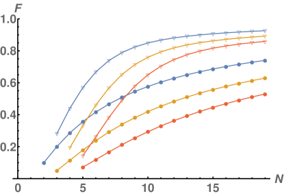
Figure 8: Comparison of the first bound (9) on entanglement fidelity from Theorem 2 in the main text (full circles (full circles, for k=2k=2 marked with Refer to caption, k=3k=3 Refer to caption, k=4k=4 Refer to caption)) with exact values for the qubit case (reversed triangle markers, for k=2k=2 marked with Refer to caption, k=3k=3 Refer to caption, k=4k=4 Refer to caption).

In case of probability of success, using directly the argumentation from Section V, we rewrite expression (66) as:

psucc(N,k)=12Ns=0(12)Nk2minjN!(2s+1)2(N/2j)!(N/2+j+1)!=12Ns=0(12)Nk2N!(2s+1)2(N/2sk/2)!(N/2+s+k/2+1)!.p_{succ}(N,k)=\frac{1}{2^{N}}\sum_{s=0(\frac{1}{2})}^{\frac{N-k}{2}}\min_{j}\frac{N!(2s+1)^{2}}{(N/2-j)!(N/2+j+1)!}=\frac{1}{2^{N}}\sum_{s=0(\frac{1}{2})}^{\frac{N-k}{2}}\frac{N!(2s+1)^{2}}{(N/2-s-k/2)!(N/2+s+k/2+1)!}. (71)

Observing that

N!(N/2sk/2)!(N/2+s+k/2+1)!=1N+1(N+1Nk2s).\frac{N!}{(N/2-s-k/2)!(N/2+s+k/2+1)!}=\frac{1}{N+1}\binom{N+1}{\frac{N-k}{2}-s}. (72)

we get the final form given in by the following equation

psucc(N,k)=12Ns=0(12)Nk21N+1(N+1Nk2s).p_{succ}(N,k)=\frac{1}{2^{N}}\sum_{s=0(\frac{1}{2})}^{\frac{N-k}{2}}\frac{1}{N+1}\binom{N+1}{\frac{N-k}{2}-s}. (73)

In Section D of this appendix we discuss additional properties of probability of success psuccp_{succ}.

Appendix D Bounds for finite number of ports NN

To achieve our goals in this section we have combined in a non-trivial way advanced tools emerging from statistical analysis. Motivated by Berry-Essen Theorem [6, 10], which quantifies the rate of convergence to normal distribution, together with Central Limit Theorem type reasoning we express probability of success in terms of Gaussian integrals. In particular, starting from expression (73) in the finite case, we provide useful lower and upper bounds on probability of success of the perfect transmission in MPBT protocol. We can observe, that it closely resembles the expression for the probability distribution function of the distribution of number of successes in N+1N+1 Bernoulli trials each with p=1/2p=1/2. We start from proving the following:

Proposition 18.

Let k=aN,a(0,2).k=a\sqrt{N},a\in(0,2). Then

2(0x212πe(x+aNN+1)22𝑑xM(N)I1B(N)I2B(N))δB(N)psucc\displaystyle 2\left(\int_{0}^{\infty}x^{2}\frac{1}{\sqrt{2\pi}}\operatorname{e}^{-\frac{(x+a\sqrt{\frac{N}{N+1}})^{2}}{2}}dx-M(N)-I_{1}^{B}(N)-I_{2}^{B}(N)\right)-\delta^{B}(N)\leq p_{succ}\leq 2(0x212πe(x+aNN+1)22𝑑x+M(N)),\displaystyle 2\left(\int_{0}^{\infty}x^{2}\frac{1}{\sqrt{2\pi}}\operatorname{e}^{-\frac{(x+a\sqrt{\frac{N}{N+1}})^{2}}{2}}dx+M(N)\right), (74)

where

M(N)=2eN+112π,I1B(N)=(N+1)3212π,I2B(N)=(N+12π+1)e(N+11)22,δB(N)=4N1/4+11N+1e(N5/81)2N+1.\begin{split}M(N)&=\frac{2}{\operatorname{e}\sqrt{N+1}}\frac{1}{\sqrt{2\pi}},\quad I_{1}^{B}(N)=(N+1)^{-\frac{3}{2}}\frac{1}{\sqrt{2\pi}},\\ I_{2}^{B}(N)&=\left(\frac{\sqrt{N+1}}{\sqrt{2\pi}}+1\right)\operatorname{e}^{-\frac{\left(\sqrt{N+1}-1\right)^{2}}{2}},\\ \delta^{B}(N)&=4N^{-1/4}+11\sqrt{N+1}\operatorname{e}^{-\frac{\left(N^{5/8}-1\right)^{2}}{N+1}}.\end{split} (75)

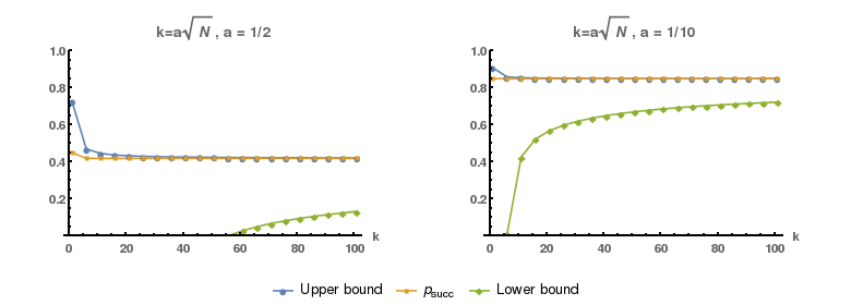
The reasoning above applies to finite number of ports. We can see the convergence of these bounds in Figure 9
Refer to caption
Figure 9: The figures present lower and upper bounds for psuccp_{succ} given in Proposition 18, for two different values of aa, where the number of teleported qubits is given by k=aNk~=~a\sqrt{N}.

Taking the limit NN\rightarrow\infty we can formulate the following

Corollary 19.

The limiting value of psuccp_{succ}, where k=aN,a(0,1),Nk=a\sqrt{N},a\in(0,1),N\rightarrow\infty is

limNpsucc=20x212πe(x+a)22𝑑x.\lim_{N\to\infty}p_{succ}=2\int_{0}^{\infty}x^{2}\frac{1}{\sqrt{2\pi}}\operatorname{e}^{-\frac{(x+a)^{2}}{2}}dx. (76)

When we take k=o(N)k=o(\sqrt{N}), i.e. k/N0k/\sqrt{N}\to 0 when N0N\to 0, we can apply the bounds (131)-(133) substituting aNN+1a\sqrt{\frac{N}{N+1}} with k/Nk/\sqrt{N}, and when we take the limit NN\to\infty we obtain

Corollary 20.

When k=o(N)k=o(\sqrt{N}) then the limit of psuccp_{succ} is

limNpsucc=20x212πex22𝑑x=1.\lim_{N\to\infty}p_{succ}=2\int_{0}^{\infty}x^{2}\frac{1}{\sqrt{2\pi}}\operatorname{e}^{-\frac{x^{2}}{2}}dx=1. (77)
Proof of Proposition 18.

The probability of success in the multi-port teleportation scheme, for even NN can be written as:

ps=1N+1s=0Nk2(2s+1)2Pr(X=Nk2s).p_{s}=\frac{1}{N+1}\sum_{s=0}^{\frac{N-k}{2}}(2s+1)^{2}\operatorname{Pr}\left(X=\frac{N-k}{2}-s\right). (78)

Instead of using discrete probability distribution Pr(Xl)\operatorname{Pr}(X\leq l) we can approximate it by Gaussian distribution Φ(lN+1212N+1)\Phi\left(\frac{l-\frac{N+1}{2}}{\frac{1}{2}\sqrt{N+1}}\right). The error of such estimation is known due to the Berry-Essen Theorem [6, 10], which in our case reads as

l=0,,N+1|Pr(Xl)Φ(lN+1212N+1)|4cN+1.\forall\ l=0,\ldots,N+1\quad\left|\operatorname{Pr}(X\leq l)-\Phi\left(\frac{l-\frac{N+1}{2}}{\frac{1}{2}\sqrt{N+1}}\right)\right|\leq\frac{4c}{\sqrt{N+1}}. (79)

The real constant cc can be analytically bounded from below and due to [11] there is c10+362π0.4097c\geq\frac{\sqrt{10}+3}{6\sqrt{2\pi}}\approx 0.4097. In this paper for our purposes we set c=1/2c=1/2. We can rewrite Φ(lN+1212N+1)\Phi\left(\frac{l-\frac{N+1}{2}}{\frac{1}{2}\sqrt{N+1}}\right) as

Φ(lN+1212N+1)=N12G(0,σ=12N+1,x)dx+i=0lN+i2N+i2+1G(0,12N+1,x)dx.\Phi\left(\frac{l-\frac{N+1}{2}}{\frac{1}{2}\sqrt{N+1}}\right)=\int_{-\infty}^{-\frac{N-1}{2}}G\left(0,\sigma=\frac{1}{2}\sqrt{N+1};x\right)\operatorname{d}x+\sum_{i=0}^{l}\int_{-\frac{N+i}{2}}^{-\frac{N+i}{2}+1}G\left(0,\frac{1}{2}\sqrt{N+1};x\right)\operatorname{d}x. (80)

The first term of the above expression decays to 0 for NN\rightarrow\infty, more precisely we have

N12G(0,σ=12N+1,x)dx=22π(N+1)N12exp(2x2N+1)dx=22π(N+1)N12exp(2x2N+1)dxN+12exp(N+12):=G1(N),\begin{split}\int_{-\infty}^{-\frac{N-1}{2}}G\left(0,\sigma=\frac{1}{2}\sqrt{N+1};x\right)\operatorname{d}x&=\frac{2}{\sqrt{2\pi(N+1)}}\int_{-\infty}^{-\frac{N-1}{2}}\operatorname{exp}\left(-\frac{2x^{2}}{N+1}\right)\operatorname{d}x\\ &=\frac{2}{\sqrt{2\pi(N+1)}}\int_{\frac{N-1}{2}}^{\infty}\operatorname{exp}\left(-\frac{2x^{2}}{N+1}\right)\operatorname{d}x\\ &\leq\sqrt{\frac{N+1}{2}}\operatorname{exp}\left(-\frac{N+1}{2}\right):=G_{1}(N),\end{split} (81)

since the Hoeffding bound states

rexp(c~2x2)dxπc~exp(c~2r2).\int_{r}^{\infty}\operatorname{exp}(-\widetilde{c}^{2}x^{2})\operatorname{d}x\leq\frac{\sqrt{\pi}}{\widetilde{c}}\operatorname{exp}\left(-\widetilde{c}^{2}r^{2}\right). (82)

Notice that factor G1(N)G_{1}(N) decays to 0 for NN\rightarrow\infty. Now, due to (81), we have l=0,,N+1\forall\ l=0,\ldots,N+1

|Pr(Xl)Φ(lN+1212N+1)||Pr(Xl)i=0lN+i2N+i2+1G(0,12N+1,x)dx|+G1(N)=|i=0lPr(X=i)i=0lN+i2N+i2+1G(0,12N+1,x)dx|+G1(N)=i=0l|Pr(X=i)N+i2N+i2+1G(0,12N+1,x)dx|+G1(N).\begin{split}\left|\operatorname{Pr}(X\leq l)-\Phi\left(\frac{l-\frac{N+1}{2}}{\frac{1}{2}\sqrt{N+1}}\right)\right|&\leq\left|\operatorname{Pr}(X\leq l)-\sum_{i=0}^{l}\int_{-\frac{N+i}{2}}^{-\frac{N+i}{2}+1}G\left(0,\frac{1}{2}\sqrt{N+1};x\right)\operatorname{d}x\right|+G_{1}(N)\\ &=\left|\sum_{i=0}^{l}\operatorname{Pr}(X=i)-\sum_{i=0}^{l}\int_{-\frac{N+i}{2}}^{-\frac{N+i}{2}+1}G\left(0,\frac{1}{2}\sqrt{N+1};x\right)\operatorname{d}x\right|+G_{1}(N)\\ &=\sum_{i=0}^{l}\left|\operatorname{Pr}(X=i)-\int_{-\frac{N+i}{2}}^{-\frac{N+i}{2}+1}G\left(0,\frac{1}{2}\sqrt{N+1};x\right)\operatorname{d}x\right|+G_{1}(N).\end{split} (83)

Getting back to probability of success in (78):

2N+1s=0Nk2(2s+1)2Φσ(k2s12,k2s+12)ps=2N+1s=0Nk2(2s+1)2Pr(X=Nk2s)2N+1(s=0Nk2(2s+1)2Φσ(k2s12,k2s+12)s=0Nk2(2s+1)2δs),\begin{split}\frac{2}{N+1}\sum_{s=0}^{\frac{N-k}{2}}(2s+1)^{2}&\Phi_{\sigma}\left(-\frac{k}{2}-s-\frac{1}{2},-\frac{k}{2}-s+\frac{1}{2}\right)\geq\\ p_{s}&=\frac{2}{N+1}\sum_{s=0}^{\frac{N-k}{2}}(2s+1)^{2}\operatorname{Pr}\left(X=\frac{N-k}{2}-s\right)\\ &\geq\frac{2}{N+1}\left(\sum_{s=0}^{\frac{N-k}{2}}(2s+1)^{2}\Phi_{\sigma}\left(-\frac{k}{2}-s-\frac{1}{2},-\frac{k}{2}-s+\frac{1}{2}\right)-\sum_{s=0}^{\frac{N-k}{2}}(2s+1)^{2}\delta_{s}\right),\end{split} (84)

where

δs=|Pr(x=Nk2s)Φσ(k2s12,k2s+12)|,σ=12N+1.\delta_{s}=\left|\operatorname{Pr}\left(x=\frac{N-k}{2}-s\right)-\Phi_{\sigma}\left(-\frac{k}{2}-s-\frac{1}{2},-\frac{k}{2}-s+\frac{1}{2}\right)\right|,\qquad\sigma=\frac{1}{2}\sqrt{N+1}. (85)

The upper bound comes from the Lemma 7.2 from [26]. Since XB(N+1,12)X\sim B(N+1,\frac{1}{2})

Φσ(k2s12,k2s+12)Pr(X=Nk2s)\Phi_{\sigma}\left(-\frac{k}{2}-s-\frac{1}{2},-\frac{k}{2}-s+\frac{1}{2}\right)\geq\operatorname{Pr}\left(X=\frac{N-k}{2}-s\right) (86)

if

N+12+1N+1(Nk2s)\frac{N+1}{2}+1\leq N+1-\left(\frac{N-k}{2}-s\right) (87)

which is equivalent to k+2s1k+2s\geq 1 which clearly holds for kk and ss in question.

At this point we can divide further considerations into two main steps:

  1. 1.

    Showing that 2N+1s=0Nk2(2s+1)2δs0\frac{2}{N+1}\sum_{s=0}^{\frac{N-k}{2}}(2s+1)^{2}\delta_{s}\rightarrow 0 for NN\rightarrow\infty in (84).

  2. 2.

    Evaluating the first term 2N+1s=0Nk2(2s+1)2Φσ(k2s12,k2s+12)\frac{2}{N+1}\sum_{s=0}^{\frac{N-k}{2}}(2s+1)^{2}\Phi_{\sigma}\left(-\frac{k}{2}-s-\frac{1}{2},-\frac{k}{2}-s+\frac{1}{2}\right) from expression (84) in the asymptotic regime NN\rightarrow\infty.

Showing decaying of the second term in (84).
Let us focus on the first point. We write

2N+1s=0Nk2(2s+1)2δs=2N+1s=0m(N)(2s+1)2δsA+2N+1s=m(N)Nk2(2s+1)2δsB.\begin{split}\frac{2}{N+1}\sum_{s=0}^{\frac{N-k}{2}}(2s+1)^{2}\delta_{s}=\underbrace{\frac{2}{N+1}\sum_{s=0}^{m(N)}(2s+1)^{2}\delta_{s}}_{A}+\underbrace{\frac{2}{N+1}\sum_{s=m(N)}^{\frac{N-k}{2}}(2s+1)^{2}\delta_{s}}_{B}.\end{split} (88)

Substituting m(N)=(1/2)(b(N)N1)m(N)=(1/2)(b(N)\sqrt{N}-1), using fact s=0Nk2δs4cN+1\sum_{s=0}^{\frac{N-k}{2}}\delta_{s}\leq\frac{4c}{\sqrt{N+1}} with c=1/2c=1/2, we bound AA as

A2(2m(N)+1)2N+1s=0m(N)δs4b2(N)N(N+1)3/24Nb2(N)N3/2=4N1/4,A\leq\frac{2(2m(N)+1)^{2}}{N+1}\sum_{s=0}^{m(N)}\delta_{s}\leq\frac{4b^{2}(N)N}{(N+1)^{3/2}}\leq\frac{4Nb^{2}(N)}{N^{3/2}}=4N^{-1/4}, (89)

where we choose for example b(N)=N1/8b(N)=N^{1/8} getting demanded asymptotic. For the factor BB, first we write

δsPr(x=Nk2s)+Φσ(k2s12,k2s+12)Pr(xNk2s)+Φσ(k2s+12)exp((k+2s+1)22(N+1))+exp((k+2s1)22(N+1))2exp((k+2s1)22(N+1)).\begin{split}\delta_{s}&\leq\operatorname{Pr}\left(x=\frac{N-k}{2}-s\right)+\Phi_{\sigma}\left(-\frac{k}{2}-s-\frac{1}{2},-\frac{k}{2}-s+\frac{1}{2}\right)\\ &\leq\operatorname{Pr}\left(x\leq\frac{N-k}{2}-s\right)+\Phi_{\sigma}\left(-\frac{k}{2}-s+\frac{1}{2}\right)\\ &\leq\operatorname{exp}\left(-\frac{(k+2s+1)^{2}}{2(N+1)}\right)+\operatorname{exp}\left(-\frac{(k+2s-1)^{2}}{2(N+1)}\right)\\ &\leq 2\operatorname{exp}\left(-\frac{(k+2s-1)^{2}}{2(N+1)}\right).\end{split} (90)

Indeed, for Φσ(k2s+12)\Phi_{\sigma}\left(-\frac{k}{2}-s+\frac{1}{2}\right) we use σ=12N+1\sigma=\frac{1}{2}\sqrt{N+1} and the Hoeffding bound (82):

Φσ(k2s+12)=12πσk2s+12exp(12x2σ2)dxexp(12(k2s+12)2σ2)=exp((k+2s1)22(N+1)),\begin{split}\Phi_{\sigma}\left(-\frac{k}{2}-s+\frac{1}{2}\right)=\frac{1}{\sqrt{2\pi}\sigma}\int_{-\frac{k}{2}-s+\frac{1}{2}}^{\infty}\operatorname{exp}\left(-\frac{1}{2}\frac{x^{2}}{\sigma^{2}}\right)\operatorname{d}x&\leq\operatorname{exp}\left(-\frac{1}{2}\frac{(-\frac{k}{2}-s+\frac{1}{2})^{2}}{\sigma^{2}}\right)\\ &=\operatorname{exp}\left(-\frac{(k+2s-1)^{2}}{2(N+1)}\right),\end{split} (91)

For Pr(xNk2s)\operatorname{Pr}\left(x\leq\frac{N-k}{2}-s\right) we use the Chernoff bound Pr(X<(1δ)μ)eμδ22\operatorname{Pr}(X<(1-\delta)\mu)\leq\operatorname{e}^{-\frac{\mu\delta^{2}}{2}}, with μ=N+1\mu=N+1 and 1δ=Nk2sN+11-\delta=\frac{N-k-2s}{N+1}:

Pr(xNk2s)exp((k+2s+1)22(N+1)).\operatorname{Pr}\left(x\leq\frac{N-k}{2}-s\right)\leq\operatorname{exp}\left(-\frac{(k+2s+1)^{2}}{2(N+1)}\right). (92)

Applying (90) to BB we reduce to

B4N+1s=m(N)Nk2(2s+1)2exp((k+2s1)22(N+1))4(Nk+1)N+1s=m(N)Nk2exp((k+2s1)22(N+1))4(Nk+1)N+1s=m(N)exp((k+2s1)22(N+1))4s=m(N)exp((k+2s1)22(N+1))11N+1exp((k+2m(N)1)22(N+1))11N+1exp(2m2(N)N+1),\begin{split}B\leq\frac{4}{N+1}\sum_{s=m(N)}^{\frac{N-k}{2}}(2s+1)^{2}\operatorname{exp}\left(-\frac{(k+2s-1)^{2}}{2(N+1)}\right)&\leq\frac{4(N-k+1)}{N+1}\sum_{s=m(N)}^{\frac{N-k}{2}}\operatorname{exp}\left(-\frac{(k+2s-1)^{2}}{2(N+1)}\right)\\ &\leq\frac{4(N-k+1)}{N+1}\sum_{s=m(N)}^{\infty}\operatorname{exp}\left(-\frac{(k+2s-1)^{2}}{2(N+1)}\right)\\ &\leq 4\sum_{s=m(N)}^{\infty}\operatorname{exp}\left(-\frac{(k+2s-1)^{2}}{2(N+1)}\right)\\ &\leq\frac{11}{\sqrt{N+1}}\operatorname{exp}\left(-\frac{(k+2m(N)-1)^{2}}{2(N+1)}\right)\\ &\leq 11\sqrt{N+1}\operatorname{exp}\left(-\frac{2m^{2}(N)}{N+1}\right),\end{split} (93)

where in the fourth inequality we use the Hoeffding inequality. Finally, using explicit form of the function m(N)=(1/2)(N5/81)m(N)=(1/2)(N^{5/8}-1) and expression (89) we bound left-hand side of (88) as

2N+1s=0Nk2(2s+1)2δs4N3/2+11N+1exp((N5/81)2N+1)\frac{2}{N+1}\sum_{s=0}^{\frac{N-k}{2}}(2s+1)^{2}\delta_{s}\leq 4N^{-3/2}+11\sqrt{N+1}\operatorname{exp}\left(-\frac{\left(N^{5/8}-1\right)^{2}}{N+1}\right) (94)

which clearly decays to 0 with NN\rightarrow\infty. It means psp_{s} in (84) can be bounded from the below

ps2N+1s=0Nk2(2s+1)2Φσ(k2s12,k2s+12)4N1/411N+1exp((N5/81)2N+1).\begin{split}p_{s}&\geq\frac{2}{N+1}\sum_{s=0}^{\frac{N-k}{2}}(2s+1)^{2}\Phi_{\sigma}\left(-\frac{k}{2}-s-\frac{1}{2},-\frac{k}{2}-s+\frac{1}{2}\right)-4N^{-1/4}-11\sqrt{N+1}\operatorname{exp}\left(-\frac{\left(N^{5/8}-1\right)^{2}}{N+1}\right).\end{split} (95)

Estimation of the first term in (84). We now want to estimate the expression

2N+1(s=0Nk2(2s+1)2Φσ(k2s12,k2s+12)).\frac{2}{N+1}\left(\sum_{s=0}^{\frac{N-k}{2}}(2s+1)^{2}\Phi_{\sigma}\left(-\frac{k}{2}-s-\frac{1}{2},-\frac{k}{2}-s+\frac{1}{2}\right)\right). (96)

First, we can write

2N+1(s=0Nk2(2s+1)2Φσ(k2s12,k2s+12,))=2N+1s=0Nk2(2s+1)2k2s12k2s+1222π(N+1)e2x2N+1dx\displaystyle\frac{2}{N+1}\left(\sum_{s=0}^{\frac{N-k}{2}}(2s+1)^{2}\Phi_{\sigma}\left(-\frac{k}{2}-s-\frac{1}{2},-\frac{k}{2}-s+\frac{1}{2},\right)\right)=\frac{2}{N+1}\sum_{s=0}^{\frac{N-k}{2}}(2s+1)^{2}\int_{-\frac{k}{2}-s-\frac{1}{2}}^{-\frac{k}{2}-s+\frac{1}{2}}\frac{2}{\sqrt{2\pi(N+1)}}\operatorname{e}^{-\frac{2x^{2}}{N+1}}dx (97)
2N+1s=0Nk2(2s+1)222π(N+1)e(k+2s+1)22(N+1)\displaystyle\geq\frac{2}{N+1}\sum_{s=0}^{\frac{N-k}{2}}(2s+1)^{2}\frac{2}{\sqrt{2\pi(N+1)}}\operatorname{e}^{-\frac{(k+2s+1)^{2}}{2(N+1)}} (98)
=22N+1s=0Nk2(1N+1+s2N+1)212πe(1N+1+s2N+1+kN+1)22.\displaystyle=2\frac{2}{\sqrt{N+1}}\sum_{s=0}^{\frac{N-k}{2}}\left(\frac{1}{\sqrt{N+1}}+s\frac{2}{\sqrt{N+1}}\right)^{2}\frac{1}{\sqrt{2\pi}}\operatorname{e}^{-\frac{\left(\frac{1}{\sqrt{N+1}}+s\frac{2}{\sqrt{N+1}}+\frac{k}{\sqrt{N+1}}\right)^{2}}{2}}. (99)

where we replace integral over interval [k2s12,k2s+12][{-\frac{k}{2}-s-\frac{1}{2}},{-\frac{k}{2}-s+\frac{1}{2}}] with local minimum of integrated function multiplied by the length of the interval, which is 11. One can identify the last expression as a Riemann left-sum of function

fN(z)z2e(z+kN+1)22f^{N}(z)\coloneqq z^{2}\operatorname{e}^{\frac{(z+\frac{k}{\sqrt{N+1}})^{2}}{2}} (100)

on the interval [1N+1,NkN+1][\frac{1}{\sqrt{N+1}},\frac{N-k}{\sqrt{N+1}}]. We will transform this sum in the manner depicted in Figure 10. Setting k=aNk=a\sqrt{N} the target function takes form

fN(z)=z2e(z+aNN+1)22.f^{N}(z)=z^{2}\operatorname{e}^{\frac{(z+a\sqrt{\frac{N}{N+1}})^{2}}{2}}. (101)

One can check, that for

0zmNN+1a+NN+1a2+820\leq z\leq m\coloneqq\frac{-\sqrt{\frac{N}{N+1}}a+\sqrt{\frac{N}{N+1}a^{2}+8}}{2} (102)

it is monotonically increasing, while for zmz\geq m it decreases. Therefore it can be split into two components: one consisting of partitions {[1N+1,1+2sN+1],s0,,sm}\{[\frac{1}{\sqrt{N+1}},\frac{1+2s}{\sqrt{N+1}}],s\in 0,\dots,s_{m}\} where 1+2smN+1m\frac{1+2s_{m}}{\sqrt{N+1}}\leq m, and the other consisting of partitions for higher values of ss. Thus we have

2N+1s=0Nk2\displaystyle\frac{2}{\sqrt{N+1}}\sum_{s=0}^{\frac{N-k}{2}} (1N+1+s2N+1)212πe(1N+1+s2N+1+kN+1)22\displaystyle\left(\frac{1}{\sqrt{N+1}}+s\frac{2}{\sqrt{N+1}}\right)^{2}\frac{1}{\sqrt{2\pi}}\operatorname{e}^{-\frac{\left(\frac{1}{\sqrt{N+1}}+s\frac{2}{\sqrt{N+1}}+\frac{k}{\sqrt{N+1}}\right)^{2}}{2}} (103)
=\displaystyle= 22N+1s=0sm(1N+1+s2N+1)212πe(1N+1+s2N+1+kN+1)22\displaystyle 2\frac{2}{\sqrt{N+1}}\sum_{s=0}^{s_{m}}\left(\frac{1}{\sqrt{N+1}}+s\frac{2}{\sqrt{N+1}}\right)^{2}\frac{1}{\sqrt{2\pi}}\operatorname{e}^{-\frac{\left(\frac{1}{\sqrt{N+1}}+s\frac{2}{\sqrt{N+1}}+\frac{k}{\sqrt{N+1}}\right)^{2}}{2}} (104)
+22N+1s=sm+1Nk2(1N+1+s2N+1)212πe(1N+1+s2N+1+kN+1)22\displaystyle+2\frac{2}{\sqrt{N+1}}\sum_{s=s_{m}+1}^{\frac{N-k}{2}}\left(\frac{1}{\sqrt{N+1}}+s\frac{2}{\sqrt{N+1}}\right)^{2}\frac{1}{\sqrt{2\pi}}\operatorname{e}^{-\frac{\left(\frac{1}{\sqrt{N+1}}+s\frac{2}{\sqrt{N+1}}+\frac{k}{\sqrt{N+1}}\right)^{2}}{2}} (105)
=\displaystyle= SLN(1N+1,1+2(sm+1)N+1)+SLN(1+2(sm+1)N+1,NaN+1N+1),\displaystyle S_{L}^{N}\left(\frac{1}{\sqrt{N+1}},\frac{1+2(s_{m}+1)}{\sqrt{N+1}}\right)+S_{L}^{N}\left(\frac{1+2(s_{m}+1)}{\sqrt{N+1}},\frac{N-a\sqrt{N}+1}{\sqrt{N+1}}\right), (106)

where SLN(1N+1,1+2(sm+1)N+1)S_{L}^{N}\left(\frac{1}{\sqrt{N+1}},\frac{1+2(s_{m}+1)}{\sqrt{N+1}}\right) denotes left Riemann sum on the interval [1N+1,1+(2sm+1)N+1][\frac{1}{\sqrt{N+1}},\frac{1+(2s_{m}+1)}{\sqrt{N+1}}]. Setting t=s+1t=s+1, we can write

SLN(1N+1,2sm+1N+1)\displaystyle S_{L}^{N}\left(\frac{1}{\sqrt{N+1}},\frac{2s_{m}+1}{\sqrt{N+1}}\right) =22N+1s=0sm(1N+1+s2N+1)212πe(1N+1+s2N+1+kN+1)22\displaystyle=2\frac{2}{\sqrt{N+1}}\sum_{s=0}^{s_{m}}\left(\frac{1}{\sqrt{N+1}}+s\frac{2}{\sqrt{N+1}}\right)^{2}\frac{1}{\sqrt{2\pi}}\operatorname{e}^{-\frac{\left(\frac{1}{\sqrt{N+1}}+s\frac{2}{\sqrt{N+1}}+\frac{k}{\sqrt{N+1}}\right)^{2}}{2}} (107)
=22N+1t=1tm(1N+1+t2N+1)212πe(1N+1+t2N+1+kN+1)22\displaystyle=2\frac{2}{\sqrt{N+1}}\sum_{t=1}^{t_{m}}\left(-\frac{1}{\sqrt{N+1}}+t\frac{2}{\sqrt{N+1}}\right)^{2}\frac{1}{\sqrt{2\pi}}\operatorname{e}^{-\frac{\left(-\frac{1}{\sqrt{N+1}}+t\frac{2}{\sqrt{N+1}}+\frac{k}{\sqrt{N+1}}\right)^{2}}{2}} (108)
=SRN(1N+1,1+tmN+1).\displaystyle=S_{R}^{N}\left(-\frac{1}{\sqrt{N+1}},\frac{-1+t_{m}}{\sqrt{N+1}}\right). (109)

Thus

SLN(1N+1,1+2(sm+1)N+1)+SLN(1+2(sm+1)N+1,NaN+1N+1)\displaystyle S_{L}^{N}\left(\frac{1}{\sqrt{N+1}},\frac{1+2(s_{m}+1)}{\sqrt{N+1}}\right)+S_{L}^{N}\left(\frac{1+2(s_{m}+1)}{\sqrt{N+1}},\frac{N-a\sqrt{N}+1}{\sqrt{N+1}}\right) (110)
=SRN(1N+1,1+2tmN+1)+SLN(1+2(sm+1)N+1,NaN+1N+1).\displaystyle=S_{R}^{N}\left(-\frac{1}{\sqrt{N+1}},\frac{-1+2t_{m}}{\sqrt{N+1}}\right)+S_{L}^{N}\left(\frac{1+2(s_{m}+1)}{\sqrt{N+1}},\frac{N-a\sqrt{N}+1}{\sqrt{N+1}}\right). (111)

We can observe, that we shifted the first left sum by 2N+1-\frac{2}{\sqrt{N+1}}, which corresponds to single partition interval, turning it into right sum. Supplementing the upper bound of the "missing middle term" 2N+1m212πe(m+kN+1)22\frac{2}{\sqrt{N+1}}m^{2}\frac{1}{\sqrt{2\pi}}\operatorname{e}^{-\frac{\left(m+\frac{k}{\sqrt{N+1}}\right)^{2}}{2}}, we obtain the following restriction

SRN(1N+1,1+2tmN+1)+SLN(1+2(sm+1)N+1,NaN+1N+1)+2N+1m212πe(m+kN+1)22dx\displaystyle S_{R}^{N}\left(-\frac{1}{\sqrt{N+1}},\frac{-1+2t_{m}}{\sqrt{N+1}}\right)+S_{L}^{N}\left(\frac{1+2(s_{m}+1)}{\sqrt{N+1}},\frac{N-a\sqrt{N}+1}{\sqrt{N+1}}\right)+\frac{2}{\sqrt{N+1}}m^{2}\frac{1}{\sqrt{2\pi}}\operatorname{e}^{-\frac{\left(m+\frac{k}{\sqrt{N+1}}\right)^{2}}{2}}dx (112)
1N+1NaN+1N+1x212πe(x+aNN+1)22𝑑x\displaystyle\geq\int_{-\frac{1}{\sqrt{N+1}}}^{\frac{N-a\sqrt{N}+1}{\sqrt{N+1}}}x^{2}\frac{1}{\sqrt{2\pi}}\operatorname{e}^{-\frac{(x+a\sqrt{\frac{N}{N+1}})^{2}}{2}}dx (113)
1N+1NaN+1N+1x212πe(x+aNN+1)22𝑑x.\displaystyle\geq\int_{\frac{1}{\sqrt{N+1}}}^{\frac{N-a\sqrt{N}+1}{\sqrt{N+1}}}x^{2}\frac{1}{\sqrt{2\pi}}\operatorname{e}^{-\frac{(x+a\sqrt{\frac{N}{N+1}})^{2}}{2}}dx. (114)

These three sums are depicted in Figure 10.
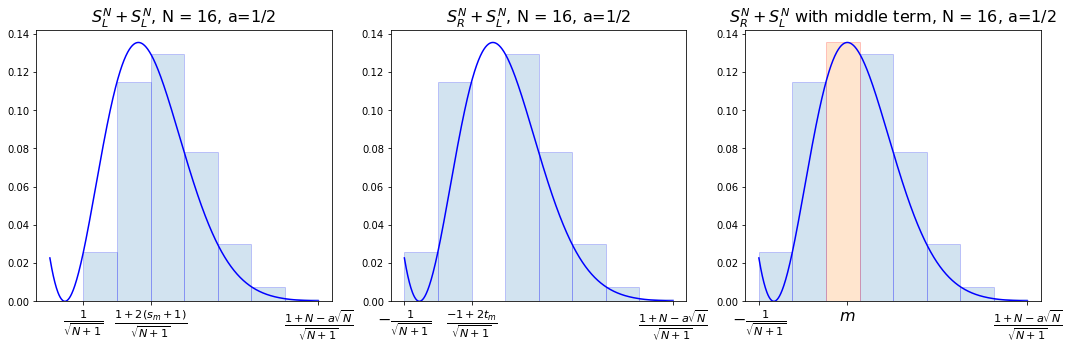
Refer to caption
Figure 10: Three Riemann sums: (110), (111) and (112).

Thus the initial Riemann sum (110) is bounded by

2N+1s=0Nk2\displaystyle\frac{2}{\sqrt{N+1}}\sum_{s=0}^{\frac{N-k}{2}} (1N+1+s2N+1)212πe(1N+1+s2N+1+kN+1)22\displaystyle\left(\frac{1}{\sqrt{N+1}}+s\frac{2}{\sqrt{N+1}}\right)^{2}\frac{1}{\sqrt{2\pi}}\operatorname{e}^{-\frac{\left(\frac{1}{\sqrt{N+1}}+s\frac{2}{\sqrt{N+1}}+\frac{k}{\sqrt{N+1}}\right)^{2}}{2}} (115)
=SLN(1N+1,2sm+3N+1)+SLN(2sm+3N+1,NaN+1N+1)\displaystyle=S_{L}^{N}\left(\frac{1}{\sqrt{N+1}},\frac{2s_{m}+3}{\sqrt{N+1}})+S_{L}^{N}(\frac{2s_{m}+3}{\sqrt{N+1}},\frac{N-a\sqrt{N}+1}{\sqrt{N+1}}\right) (116)
=SRN(1N+1,2sm+1N+1)+SLN(2sm+3N+1,NaN+1N+1)\displaystyle=S_{R}^{N}\left(-\frac{1}{\sqrt{N+1}},\frac{2s_{m}+1}{\sqrt{N+1}})+S_{L}^{N}(\frac{2s_{m}+3}{\sqrt{N+1}},\frac{N-a\sqrt{N}+1}{\sqrt{N+1}}\right) (117)
1N+1NaN+1N+1x212πe(x+aNN+1)22𝑑x2N+1m212πe(m+kN+1)22\displaystyle\geq\int_{\frac{1}{\sqrt{N+1}}}^{\frac{N-a\sqrt{N}+1}{\sqrt{N+1}}}x^{2}\frac{1}{\sqrt{2\pi}}\operatorname{e}^{-\frac{(x+a\sqrt{\frac{N}{N+1}})^{2}}{2}}dx-\frac{2}{\sqrt{N+1}}m^{2}\frac{1}{\sqrt{2\pi}}\operatorname{e}^{\frac{\left(m+\frac{k}{\sqrt{N+1}}\right)^{2}}{2}} (118)
1N+1NaN+1N+1x212πe(x+aNN+1)22𝑑x2N+1m212πem22\displaystyle\geq\int_{\frac{1}{\sqrt{N+1}}}^{\frac{N-a\sqrt{N}+1}{\sqrt{N+1}}}x^{2}\frac{1}{\sqrt{2\pi}}\operatorname{e}^{-\frac{(x+a\sqrt{\frac{N}{N+1}})^{2}}{2}}dx-\frac{2}{\sqrt{N+1}}m^{2}\frac{1}{\sqrt{2\pi}}\operatorname{e}^{\frac{m^{2}}{2}} (119)
1N+1NaN+1N+1x212πe(x+aNN+1)22𝑑x4eN+112π\displaystyle\geq\int_{\frac{1}{\sqrt{N+1}}}^{\frac{N-a\sqrt{N}+1}{\sqrt{N+1}}}x^{2}\frac{1}{\sqrt{2\pi}}\operatorname{e}^{-\frac{(x+a\sqrt{\frac{N}{N+1}})^{2}}{2}}dx-\frac{4}{\operatorname{e}\sqrt{N+1}}\frac{1}{\sqrt{2\pi}} (120)
1N+1NaN+1N+1x212πe(x+aNN+1)22𝑑x2N+112π\displaystyle\geq\int_{\frac{1}{\sqrt{N+1}}}^{\frac{N-a\sqrt{N}+1}{\sqrt{N+1}}}x^{2}\frac{1}{\sqrt{2\pi}}\operatorname{e}^{-\frac{(x+a\sqrt{\frac{N}{N+1}})^{2}}{2}}dx-\frac{2}{\sqrt{N+1}}\frac{1}{\sqrt{2\pi}} (121)

and thus (96) admits the following restriction

2N+1\displaystyle\frac{2}{N+1} (s=0Nk2(2s+1)2Φσ(k2s12,k2s+12))\displaystyle\left(\sum_{s=0}^{\frac{N-k}{2}}(2s+1)^{2}\Phi_{\sigma}\left(-\frac{k}{2}-s-\frac{1}{2},-\frac{k}{2}-s+\frac{1}{2}\right)\right) (122)
22N+1s=0Nk2(1N+1+s2N+1)212πe(1N+1+s2N+1+kN+1)22\displaystyle\geq 2\frac{2}{\sqrt{N+1}}\sum_{s=0}^{\frac{N-k}{2}}\left(\frac{1}{\sqrt{N+1}}+s\frac{2}{\sqrt{N+1}}\right)^{2}\frac{1}{\sqrt{2\pi}}\operatorname{e}^{-\frac{\left(\frac{1}{\sqrt{N+1}}+s\frac{2}{\sqrt{N+1}}+\frac{k}{\sqrt{N+1}}\right)^{2}}{2}} (123)
2(1N+1NaN+1N+1x212πe(x+aNN+1)22𝑑x2N+112π).\displaystyle\geq 2\left(\int_{\frac{1}{\sqrt{N+1}}}^{\frac{N-a\sqrt{N}+1}{\sqrt{N+1}}}x^{2}\frac{1}{\sqrt{2\pi}}\operatorname{e}^{-\frac{(x+a\sqrt{\frac{N}{N+1}})^{2}}{2}}dx-\frac{2}{\sqrt{N+1}}\frac{1}{\sqrt{2\pi}}\right). (124)

Equivalent reasoning can be used to obtain the upper bound of (96). Thus, for finite NN one obtains

21N+1NaN+1N+1x212πe(x+aNN+1)22𝑑x+2Mpsucc21N+1NaN+1N+1x212πe(x+aNN+1)22𝑑x2Ms=0Nk2(2s+1)2δs,\displaystyle\displaystyle 2\int_{\frac{1}{\sqrt{N+1}}}^{\frac{N-a\sqrt{N}+1}{\sqrt{N+1}}}x^{2}\frac{1}{\sqrt{2\pi}}\operatorname{e}^{-\frac{(x+a\sqrt{\frac{N}{N+1}})^{2}}{2}}dx+2M\geq p_{succ}\geq 2\int_{\frac{1}{\sqrt{N+1}}}^{\frac{N-a\sqrt{N}+1}{\sqrt{N+1}}}x^{2}\frac{1}{\sqrt{2\pi}}\operatorname{e}^{-\frac{(x+a\sqrt{\frac{N}{N+1}})^{2}}{2}}dx-2M-\sum_{s=0}^{\frac{N-k}{2}}(2s+1)^{2}\delta_{s}, (125)

where M=2N+112πM=\frac{2}{\sqrt{N+1}}\frac{1}{\sqrt{2\pi}}. This bound can be further refined. On the one hand, clearly

1N+1NaN+1N+1x212πe(x+aNN+1)22𝑑x+M0x212πe(x+aNN+1)22𝑑x+M.\displaystyle\int_{\frac{1}{\sqrt{N+1}}}^{\frac{N-a\sqrt{N}+1}{\sqrt{N+1}}}x^{2}\frac{1}{\sqrt{2\pi}}\operatorname{e}^{-\frac{(x+a\sqrt{\frac{N}{N+1}})^{2}}{2}}dx+M\leq\displaystyle\int_{0}^{\infty}x^{2}\frac{1}{\sqrt{2\pi}}\operatorname{e}^{-\frac{(x+a\sqrt{\frac{N}{N+1}})^{2}}{2}}dx+M. (126)

On the other hand

1N+1NaN+1N+1x212πe(x+aNN+1)22dxMs=0Nk2(2s+1)2δs=0x212πe(x+aNN+1)22dxMs=0Nk2(2s+1)2δs01N+1x212πe(x+aNN+1)22dxNaN+1N+1x212πe(x+aNN+1)22dx=0x212πe(x+aNN+1)22dxMs=0Nk2(2s+1)2δsI1I2.\begin{split}&\int_{\frac{1}{\sqrt{N+1}}}^{\frac{N-a\sqrt{N}+1}{\sqrt{N+1}}}x^{2}\frac{1}{\sqrt{2\pi}}\operatorname{e}^{-\frac{(x+a\sqrt{\frac{N}{N+1}})^{2}}{2}}dx-M-\sum_{s=0}^{\frac{N-k}{2}}(2s+1)^{2}\delta_{s}=\\ &\int_{0}^{\infty}x^{2}\frac{1}{\sqrt{2\pi}}\operatorname{e}^{-\frac{(x+a\sqrt{\frac{N}{N+1}})^{2}}{2}}dx-M-\sum_{s=0}^{\frac{N-k}{2}}(2s+1)^{2}\delta_{s}-\int_{0}^{\frac{1}{\sqrt{N+1}}}x^{2}\frac{1}{\sqrt{2\pi}}\operatorname{e}^{-\frac{(x+a\sqrt{\frac{N}{N+1}})^{2}}{2}}dx-\int_{\frac{N-a\sqrt{N}+1}{\sqrt{N+1}}}^{\infty}x^{2}\frac{1}{\sqrt{2\pi}}\operatorname{e}^{-\frac{(x+a\sqrt{\frac{N}{N+1}})^{2}}{2}}dx=\\ &\int_{0}^{\infty}x^{2}\frac{1}{\sqrt{2\pi}}\operatorname{e}^{-\frac{(x+a\sqrt{\frac{N}{N+1}})^{2}}{2}}dx-M-\sum_{s=0}^{\frac{N-k}{2}}(2s+1)^{2}\delta_{s}-I_{1}-I_{2}.\end{split} (127)

One has

I1=01N+1x212πe(x+aNN+1)22𝑑x01N+1x212πex22𝑑x01N+11N+112π𝑑x=(N+1)3212πI_{1}=\int_{0}^{\frac{1}{\sqrt{N+1}}}x^{2}\frac{1}{\sqrt{2\pi}}\operatorname{e}^{-\frac{(x+a\sqrt{\frac{N}{N+1}})^{2}}{2}}dx\leq\int_{0}^{\frac{1}{\sqrt{N+1}}}x^{2}\frac{1}{\sqrt{2\pi}}\operatorname{e}^{-\frac{x^{2}}{2}}dx\leq\int_{0}^{\frac{1}{\sqrt{N+1}}}\frac{1}{N+1}\frac{1}{\sqrt{2\pi}}dx=(N+1)^{-\frac{3}{2}}\frac{1}{\sqrt{2\pi}} (128)

and having definition of the complementary error function erfc(x):=1erf(x)\operatorname{erfc}(x):=1-\operatorname{erf}(x), where erf(x):=2π0xet2dt\operatorname{erf}(x):=\frac{2}{\sqrt{\pi}}\int_{0}^{x}\operatorname{e}^{-t^{2}}dt is the error function we write

I2=NaN+1N+1x212πe(x+aNN+1)22dxNaN+1N+1x212πex22dxbx212πex22dx=beb222π+12erfc(b2)=beb222π+1πb2ex22dxbeb222π+eb22,\begin{split}I_{2}=\int_{\frac{N-a\sqrt{N}+1}{\sqrt{N+1}}}^{\infty}x^{2}\frac{1}{\sqrt{2\pi}}\operatorname{e}^{-\frac{(x+a\sqrt{\frac{N}{N+1}})^{2}}{2}}dx\leq\int_{\frac{N-a\sqrt{N}+1}{\sqrt{N+1}}}^{\infty}x^{2}\frac{1}{\sqrt{2\pi}}\operatorname{e}^{-\frac{x^{2}}{2}}dx\coloneqq\int_{b}^{\infty}x^{2}\frac{1}{\sqrt{2\pi}}\operatorname{e}^{-\frac{x^{2}}{2}}dx=\\ \frac{b\operatorname{e}^{-\frac{b^{2}}{2}}}{\sqrt{2\pi}}+\frac{1}{2}\operatorname{erfc}\left(\frac{b}{\sqrt{2}}\right)=\frac{b\operatorname{e}^{-\frac{b^{2}}{2}}}{\sqrt{2\pi}}+\frac{1}{\sqrt{\pi}}\int_{\frac{b}{\sqrt{2}}}^{\infty}\operatorname{e}^{-\frac{x^{2}}{2}}dx\leq\frac{b\operatorname{e}^{-\frac{b^{2}}{2}}}{\sqrt{2\pi}}+\operatorname{e}^{-\frac{b^{2}}{2}},\\ \end{split} (129)

where in (129) we use Hoeffiding bound, i.e. tecx2dxπcec2t2\int_{t}^{\infty}\operatorname{e}^{-cx^{2}}dx\leq\frac{\sqrt{\pi}}{c}\operatorname{e}^{-c^{2}t^{2}} and b=N+1aNN+1=N+1aNN+1b=\frac{N+1-a\sqrt{N}}{\sqrt{N+1}}=\sqrt{N+1}-a\sqrt{\frac{N}{N+1}}. Furthermore

beb222π+eb22=((N+1aNN+1)2π+1)e(N+1aNN+1)22((N+1aNN+1)2π+1)e(N+11)22(N+12π+1)e(N+11)22.\begin{split}\frac{b\operatorname{e}^{-\frac{b^{2}}{2}}}{\sqrt{2\pi}}+\operatorname{e}^{-\frac{b^{2}}{2}}=\left(\frac{\left(\sqrt{N+1}-a\sqrt{\frac{N}{N+1}}\right)}{\sqrt{2\pi}}+1\right)\operatorname{e}^{-\frac{\left(\sqrt{N+1}-a\sqrt{\frac{N}{N+1}}\right)^{2}}{2}}\leq\\ \left(\frac{\left(\sqrt{N+1}-a\sqrt{\frac{N}{N+1}}\right)}{\sqrt{2\pi}}+1\right)\operatorname{e}^{-\frac{\left(\sqrt{N+1}-1\right)^{2}}{2}}\leq\left(\frac{\sqrt{N+1}}{\sqrt{2\pi}}+1\right)\operatorname{e}^{-\frac{\left(\sqrt{N+1}-1\right)^{2}}{2}}.\end{split} (130)

Finally, taking into account (94), we can for a given NN and k=aN,a(0,1)k=a\sqrt{N},a\in(0,1) formulate the following lower and upper bounds for psuccp_{succ}:

2(0x212πe(x+aNN+1)22𝑑x+2eN+112π)psucc\displaystyle 2\left(\int_{0}^{\infty}x^{2}\frac{1}{\sqrt{2\pi}}\operatorname{e}^{-\frac{(x+a\sqrt{\frac{N}{N+1}})^{2}}{2}}dx+\frac{2}{\operatorname{e}\sqrt{N+1}}\frac{1}{\sqrt{2\pi}}\right)\geq p_{succ}\geq (131)
2(0x212πe(x+aNN+1)22𝑑x2eN+112π(N+12π+1)e(N+11)22(N+1)3212π)+\displaystyle 2\left(\int_{0}^{\infty}x^{2}\frac{1}{\sqrt{2\pi}}\operatorname{e}^{-\frac{(x+a\sqrt{\frac{N}{N+1}})^{2}}{2}}dx-\frac{2}{\operatorname{e}\sqrt{N+1}}\frac{1}{\sqrt{2\pi}}-\left(\frac{\sqrt{N+1}}{\sqrt{2\pi}}+1\right)\operatorname{e}^{-\frac{\left(\sqrt{N+1}-1\right)^{2}}{2}}-(N+1)^{-\frac{3}{2}}\frac{1}{\sqrt{2\pi}}\right)+ (132)
2N+1(4N1/4+11N+1e(N5/81)2N+1).\displaystyle-\frac{2}{N+1}\left(4N^{-1/4}+11\sqrt{N+1}\operatorname{e}^{-\frac{\left(N^{5/8}-1\right)^{2}}{N+1}}\right). (133)

References

  • Adin and Roichman [2014] Ron M. Adin and Yuval Roichman. Enumeration of standard young tableaux, 2014. URL https://arxiv.org/abs/1408.4497.
  • Aitken [1943] A. C. Aitken. Xxvi.—the monomial expansion of determinantal symmetric functions. Proceedings of the Royal Society of Edinburgh. Section A. Mathematical and Physical Sciences, 61(3):300–310, 1943. doi: 10.1017/S0080454100006312.
  • Banchi et al. [2020] Leonardo Banchi, Jason Pereira, Seth Lloyd, and Stefano Pirandola. Convex optimization of programmable quantum computers. npj Quantum Information, 6(1):42, May 2020. ISSN 2056-6387. doi: 10.1038/s41534-020-0268-2.
  • Beigi and König [2011] Salman Beigi and Robert König. Simplified instantaneous non-local quantum computation with applications to position-based cryptography. New Journal of Physics, 13(9):093036, 2011. ISSN 1367-2630. doi: 10.1088/1367-2630/13/9/093036.
  • Bennett et al. [1993] Charles H. Bennett, Gilles Brassard, Claude Crépeau, Richard Jozsa, Asher Peres, and William K. Wootters. Teleporting an unknown quantum state via dual classical and Einstein-Podolsky-Rosen channels. Physical Review Letters, 70(13):1895–1899, March 1993. doi: 10.1103/PhysRevLett.70.1895.
  • Berry [1941] Andrew C. Berry. The accuracy of the gaussian approximation to the sum of independent variates. Transactions of the American Mathematical Society, 49(1):122–136, 1941. doi: https://doi.org/10.1090/S0002-9947-1941-0003498-3.
  • Buhrman et al. [2016] Harry Buhrman, Łukasz Czekaj, Andrzej Grudka, Michał Horodecki, Paweł Horodecki, Marcin Markiewicz, Florian Speelman, and Sergii Strelchuk. Quantum communication complexity advantage implies violation of a Bell inequality. Proceedings of the National Academy of Sciences, 113(12):3191–3196, March 2016. ISSN 0027-8424, 1091-6490. doi: 10.1073/pnas.1507647113.
  • Chiribella and Ebler [2019] Giulio Chiribella and Daniel Ebler. Quantum speedup in the identification of cause-effect relations. Nature Communications, 10:1472, Apr 2019. doi: 10.1038/s41467-019-09383-8.
  • Christandl et al. [2021] Matthias Christandl, Felix Leditzky, Christian Majenz, Graeme Smith, Florian Speelman, and Michael Walter. Asymptotic performance of port-based teleportation. Communications in Mathematical Physics, 381(1):379–451, Jan 2021. ISSN 1432-0916. doi: 10.1007/s00220-020-03884-0.
  • Esseen [1942] Carl-Gustav Esseen. On the liapunoff limit of error in the theory of probability. Arkiv för Matematik, Astronomi och Fysik A28, pages 1–19, 1942.
  • Esseen [1956] Carl-Gustav Esseen. A moment inequality with an application to the central limit theorem. Scandinavian Actuarial Journal, 1956(2):160–170, 1956. doi: 10.1080/03461238.1956.10414946.
  • Fulton [1997] W. Fulton. Young Tableaux. With Applications to Representation Theory and Geometry. Cambridge University Press, New York, 1997.
  • Fulton and Harris [1991] W. Fulton and J. Harris. Representation Theory - A first Course. Springer-Verlag, New York, 1991.
  • Ishizaka and Hiroshima [2008] Satoshi Ishizaka and Tohya Hiroshima. Asymptotic Teleportation Scheme as a Universal Programmable Quantum Processor. Physical Review Letters, 101(24):240501, December 2008. doi: 10.1103/PhysRevLett.101.240501.
  • Ishizaka and Hiroshima [2009] Satoshi Ishizaka and Tohya Hiroshima. Quantum teleportation scheme by selecting one of multiple output ports. Physical Review A, 79(4):042306, April 2009. doi: 10.1103/PhysRevA.79.042306.
  • Jeong et al. [2020] Kabgyun Jeong, Jaewan Kim, and Soojoon Lee. Generalization of port-based teleportation and controlled teleportation capability. Phys. Rev. A, 102:012414, Jul 2020. doi: 10.1103/PhysRevA.102.012414.
  • Mozrzymas et al. [2014] Marek Mozrzymas, Michał Horodecki, and Michał Studziński. Structure and properties of the algebra of partially transposed permutation operators. Journal of Mathematical Physics, 55(3):032202, March 2014. ISSN 0022-2488, 1089-7658. doi: 10.1063/1.4869027.
  • Mozrzymas et al. [2018a] Marek Mozrzymas, Michał Studziński, and Michał Horodecki. A simplified formalism of the algebra of partially transposed permutation operators with applications. Journal of Physics A Mathematical General, 51(12):125202, Mar 2018a. doi: 10.1088/1751-8121/aaad15.
  • Mozrzymas et al. [2018b] Marek Mozrzymas, Michał Studziński, Sergii Strelchuk, and Michał Horodecki. Optimal port-based teleportation. New Journal of Physics, 20(5):053006, May 2018b. doi: 10.1088/1367-2630/aab8e7.
  • Mozrzymas et al. [2021] Marek Mozrzymas, Michał Studziński, and Piotr Kopszak. Optimal Multi-port-based Teleportation Schemes. Quantum, 5:477, June 2021. ISSN 2521-327X. doi: 10.22331/q-2021-06-17-477.
  • Murao et al. [1999] M. Murao, D. Jonathan, M. B. Plenio, and V. Vedral. Quantum telecloning and multiparticle entanglement. Phys. Rev. A, 59:156–161, Jan 1999. doi: 10.1103/PhysRevA.59.156.
  • Nielsen and Chuang [1997] M. A. Nielsen and Isaac L. Chuang. Programmable quantum gate arrays. Phys. Rev. Lett., 79:321–324, Jul 1997. doi: 10.1103/PhysRevLett.79.321.
  • Pereira et al. [2021] Jason Pereira, Leonardo Banchi, and Stefano Pirandola. Characterising port-based teleportation as universal simulator of qubit channels. 54(20):205301, apr 2021. doi: 10.1088/1751-8121/abe67a.
  • Pirandola et al. [2019] Stefano Pirandola, Riccardo Laurenza, Cosmo Lupo, and Jason L. Pereira. Fundamental limits to quantum channel discrimination. npj Quantum Information, 5:50, Jun 2019. doi: 10.1038/s41534-019-0162-y.
  • Quintino et al. [2019] Marco Túlio Quintino, Qingxiuxiong Dong, Atsushi Shimbo, Akihito Soeda, and Mio Murao. Reversing unknown quantum transformations: Universal quantum circuit for inverting general unitary operations. Phys. Rev. Lett., 123:210502, Nov 2019. doi: 10.1103/PhysRevLett.123.210502.
  • Schulz [2016] Jona Schulz. The optimal Berry-Esseen constant in the binomial case. PhD thesis, University of Trier, 2016. URL https://ubt.opus.hbz-nrw.de/opus45-ubtr/frontdoor/deliver/index/docId/732/file/Dissertation_Schulz.pdf.
  • Sedlák et al. [2019] Michal Sedlák, Alessandro Bisio, and Mário Ziman. Optimal Probabilistic Storage and Retrieval of Unitary Channels. \prl, 122(17):170502, May 2019. doi: 10.1103/PhysRevLett.122.170502.
  • Strelchuk et al. [2013] Sergii Strelchuk, Michał Horodecki, and Jonathan Oppenheim. Generalized Teleportation and Entanglement Recycling. Physical Review Letters, 110(1):010505, January 2013. doi: 10.1103/PhysRevLett.110.010505.
  • Studziński et al. [2017] Michał Studziński, Sergii Strelchuk, Marek Mozrzymas, and Michał Horodecki. Port-based teleportation in arbitrary dimension. Scientific Reports, 7:10871, Sep 2017. doi: 10.1038/s41598-017-10051-4.
  • Studziński et al. [2020] Michał Studziński, Marek Mozrzymas, Piotr Kopszak, and Michał Horodecki. Efficient multi-port teleportation schemes, 2020. URL https://arxiv.org/abs/2008.00984.
  • Studziński et al. [2021] Michał Studziński, Marek Mozrzymas, and Piotr Kopszak. Degradation of the resource state in port-based teleportation scheme, 2021. URL https://arxiv.org/abs/2105.14886.