Supercell-core software: a useful tool to generate an optimal supercell for vertically stacked nanomaterials

Abstract

Vertically oriented materials, such as van der Waals heterostructures, that have novel hybrid properties are crucial for fundamental scientific research and the design of new nano-devices. Currently, most available theoretical methods require applying a supercell approach with periodic boundary conditions to explore the electronic properties of such nanomaterials. Herein, we present supercell-core software, which provides a way to determine the supercell of non-commensurate lattices, in particular, van der Waals heterostructures. Although this approach is very common, most of the reported work still uses supercells that are constructed “by hand” and on a temporary basis. The developed software is designed to facilitate finding and constructing optimised supercells (i.e., with small size and minimal strain accumulation in adjacent layers) of vertically stacked lattices.

I Introduction

When a 2D crystal is placed on top of another layer (substrate) it can either adjust its position (e.g., by rotating to follow the periodic potential of the substrate), resulting in a commensurate state, or the layers can exhibit a small lattice mismatch, in which case, the interlayer binding energy (via weak van der Waals forces) can compensate for the increase in the elastic energy. Both of these occurrences may lead to experimentally observed superperiodic structures, which are commonly known as moiré patterns. Such moiré superlattices have been widely studied in the context of many different systems, including bilayer graphene Cisternas, Flores, and Vargas (2008); Ohta et al. (2012); Hunt et al. (2013); Cao et al. (2018a), trilayer graphene Zhu et al. (2020), and bilayer black phosphorus Kang et al. (2017), as well as for many heterostructures, such as graphene on hexagonal boron nitride (hBN) Decker et al. (2011); Woods et al. (2014), or bilayer transition metal dichalcogenides (TMDC) Kang et al. (2013); Alexeev et al. (2019).

Hybrid structures consisting of different types of layers connected via weak van der Waals forces represent a new class of hybrid crystals known as van der Waals heterostructures Geim (2013). These structures are of broad interest to many researchers throughout the world, due to the novel hybrid properties arising in these materials, which are distinct from their individual layer components Kunstmann et al. (2018); Cao et al. (2018b); Birowska et al. (2019). Many of these properties can be precisely controlled by rotating the two stacked atomic layers with respect to one another Cao et al. (2018b, a); Kang et al. (2017), highlighting the fact that manipulating this unique "twist angle" degree of freedom can allow for control of the nanoscale properties of such nanomaterials Carr et al. (2017); Cao et al. (2018b).

The strain itself is the subject of a new research field in solid state physics, called straintronics Bukharaev et al. (2018), in which strain engineering methods are used to develop next-generation devices for information, sensor, and energy-saving technologies. The strain-induced physical effects in nanolayers or heterostructures, such as changes in the band structure, or electronic, optical, or magnetic properties Hu, Zhou, and Dong (2017); Tamleh, Rezaei, and Jalilian (2018); Milowska, Birowska, and Majewski (2011), are fundamentally important. Understanding these relationships is a prerequisite for developing new technologies using such nanomaterials. The strain distribution can be investigated experimentally using a variety of experimental methods Woods et al. (2014); Xue et al. (2011), such as atomic force microscopy (AFM), scanning tunnelling microscopy (STM), and/or Raman spectroscopy.

Proper modelling is required in order to better understand the phenomena and underlying physics behind the structure-properties relationships. The modelling of this type of nanomaterials mostly focuses on electronic band structure calculations, and one of the most accurate ab initio methods is based on density functional theory (DFT). Widely-used software packages, such as VASP Kresse and Müller (1996); Kresse and Hafner (1993), Quantum Espresso Giannozzi and Stefano (2009), and SIESTA Soler et al. (2002), are limited in terms of their supercell approaches, because only a few hundred atoms can be considered. However, stacking adjacent layers with different lattice parameters or different lateral crystal symmetries may allow appropriate modelling of superperiodicty in very large lateral cells, or detection of aperiodic structures. Incommensurate lattices are outside the scope of the present paper. One approach directed towards describing aperiodic layered structures can be found in reference Zhu et al. (2020). In the current work, we discuss a developed approach based on commensurate lattices. We propose a supercell software capable of finding the optimal supercell, i.e., those with small size and low strain distribution. Specifically, we have developed a software package that searches through all possible superperiodicities arising from multiples of primary cells for a given rotation angle between the top and bottom 2D lattices. The software allows determination of the optimal "magic angles" between the adjacent vertically-stacked layers and the resulting moiré patterns.

There are few available builders that can handle the construction of supercells. To the best of our knowledge, those which are freely available, such as VESTA Momma and Izumi (2008), only enable ad hoc construction by hand, without finding the optimal supercell. The other capable programs, such as Quantum Wise Smidstrup et al. (2020), which has an appropriately implemented builder, must be purchased. Herein, we present the package, supercell-core, which is free of charge and allows the user to find the optimal supercell for a given twist angle and "n" number of layers constituting the van der Waals structures. To the best of our knowledge, none of the above mentioned codes, calculate the strain distribution of adjacent layers for a particular angle between the layers.

In this article, we first present the mathematical background for the software, along with explanations of the applied algorithms and discussion of relevant technical details. Then, the code is briefly described, focusing on its functionalities. Finally, we present the practical applications of the software and provide several examples.

II Computational methodology

II.1 Mathematical description

Our methodology is based on a commensurability condition, which requires long-range order in the sets of lattice planes at the interfaces of $n$ vertically stacked layers.

In order to formulate this condition mathematically, we can consider two planar lattices: A (bottom layer; substrate) and B (top layer), where lattice B is placed on top of lattice A. We denote the unit vectors of both lattices as $\mathbf{a}_{i}$ and $\mathbf{b}_{i}$, respectively, where $i\in\{1,2\}$. The task is to find two new vectors, $\mathbf{c}_{i}$, that are commensurate to both $\mathbf{a}_{i}$ and $\mathbf{b}_{i}$ Wolf and Yip (1992), such that,

$$\exists\,m_{ij}\in\mathbb{Z}\,\land\,\exists\,n_{ij}\in\mathbb{Z}:\;\mathbf{c}_{i}=\sum_{j=1}^{2}(m_{ij})^{T}\mathbf{a}_{j}=\sum_{j=1}^{2}(n_{ij})^{T}R_{\theta}\mathbf{b}_{j},$$ (1)

where $R_{\theta}$ is the 2D rotation matrix based on the rotation angle between layers, $\theta$ (Fig. 1a). Depending on the specific case, $\theta$ might be fixed, or it might be a free parameter. The angle, $\theta$, is hereafter referred to as the twist angle.

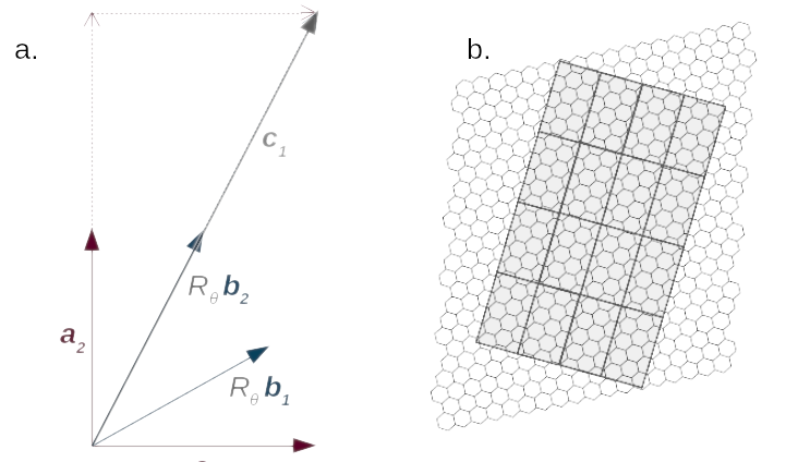
Figure 1: a. Schematic construction of a superlattice vector, $\mathbf{c}_{1}=2\mathbf{a}_{2}+\mathbf{a}_{1}=2R_{\theta}\mathbf{b}_{2}$. b. Example of two incommensurate lattices (hexagonal and rectangular).

In principle, there may be no set of integers, $m_{ij}$, $n_{ij}$, which satisfies both of the above equations, even if $\theta$ is treated as a free parameter (Fig. 1b). Thus, the commensurability condition is enforced by applying strain to the top layer. This corresponds to a linear transformation of the B lattice’s elementary cell. Note that layer A (the substrate) is always unstrained. The new task is to find the linear transformation that introduces minimal strain into the system.

For now, let us consider a fixed value of $\theta$. We denote the modified vectors of the rotated lattice B as $\mathbf{\tilde{b}}_{i}$. Then, we can define its strain tensor, $\varepsilon$, as a 2D matrix:

$$\sum_{j=1}^{2}(\varepsilon+I)^{ij}R_{\theta}\mathbf{b}_{j}=\mathbf{\tilde{b}}_{i}.$$ (2)

The $m_{ij}$ coefficients can easily be calculated given the $n_{ij}$ and $\mathbf{\tilde{b}}_{j}$ values. We must find a matrix, $\tilde{B}$, for every set of four numbers, $n_{ij}$, such that $\tilde{B}(\mathbf{b_{i}})=\mathbf{\tilde{b}}_{i}$. Then, from all sets of $n_{ij}$, we choose the one with minimal strain. To quantify the strain, we define the norm $L_{(1,1)}(\varepsilon)$, which is equal to $\sum_{ij}|\varepsilon_{ij}|$.

Note that, to find a nearly unstrained supercell for a given value of $\theta$, the software searches all possible values of $n_{ij}$ (up to some maximum value, defined by the max_el parameter in the code) in order to be certain that the optimal supercell is determined. However, this approach (hereafter referred to as the Direct algorithm), has a time complexity of $O(N^{4})$, where $N$ is the upper limit of $n_{ij}$ that is considered. However, the problem of finding a nearly unstrained supercell can be greatly simplified. It is important to note that, when the strain is zero, then $\mathbf{b}_{i}=\mathbf{\tilde{b}}_{i}$ (see Eq. 2). For every pair of $n_{i1},n_{i2}$, it is possible to write independent linear equations for $m_{i1},m_{i2}$:

$$\begin{pmatrix}\mathbf{a}_{1}&\mathbf{a}_{2}\end{pmatrix}^{-1}\begin{pmatrix}\cos\theta&-\sin\theta\\ \sin\theta&\cos\theta\end{pmatrix}\begin{pmatrix}\mathbf{b}_{1}&\mathbf{b}_{2}\end{pmatrix}\begin{pmatrix}m_{1}\\ m_{2}\end{pmatrix}=\begin{pmatrix}n_{1}\\ n_{2}\end{pmatrix}$$ (3)

The "quality" of each $n_{ij}$ pair can be assessed by taking a measure of how far the corresponding $m_{ij}$ value is from an integer solution: $\frac{\mathbf{v}-\mathrm{round}(\mathbf{v})}{||\mathbf{v}||}$, where $\mathbf{v}=\begin{pmatrix}m_{1}\\ m_{2}\end{pmatrix}$. This algorithm, known as the Fast algorithm, effectively describes $O(N^{2})$ in time complexity, and gives the same results as a direct search for cases where an optimal supercell’s strain is zero or near-zero. It can be used to find the moiré patterns or nearly unstrained unit cells. However, the Fast algorithm does not guarantee an optimal solution for cases where an optimised supercell is significantly strained. Our analysis indicates that both algorithms give the same results when the norm $L_{(1,1)}(\varepsilon)$ does not exceed a value of 0.015 (see Fig. 2). Thus, it guarantees that the strain calculated with the Fast algorithm is not overestimated.

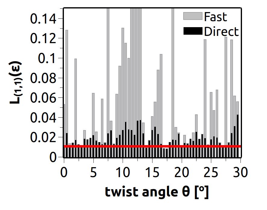
Figure 2: Comparison of the Fast and Direct algorithms implemented in the supercell-core software. The norm of the strain tensor is calculated for an optimal supercell for a phosphorene$/$graphene heterostructure as a function of the twist angle, $\theta$. The red line indicates the value of $L_{(1,1)}(\varepsilon)$=0.015, for which both algorithms give the same results. Note that, for the highly-strained lattices, the discrepancy between the algorithms can be substantial, and in those cases, use of the Direct algorithm is recommended.

These problems trivially extend to cases where $\theta$ is a free parameter, by treating it as an additional degree of freedom when searching the parameter space. When considering multiple layers, B₁, B₂, etc., we can exploit the fact that all lattices must ultimately be commensurate, and we do not modify lattice A at all. Effectively, each layer can be fit to the same lattice A supercell. Therefore, we can repeat most of the above steps for each layer independently, and record the calculated "qualities" of every set of $m_{ij}$ values for each layer. To select the final supercell (which is determined by its $m_{ij}$ coefficients), we then use the criterion of the lowest sum of the norm $L_{(1,1)}(\varepsilon)$ for all B_i layers.

II.2 Implementation

The code is implemented as a Python package using the Python numerical library, NumPy Virtanen et al. (2020). Every 2D crystal and every heterostructure is represented by a Python object. Optimisation of the strain for the given values of the twist angle, $\theta$, for each layer is carried out by first preparing a list of all possible combinations of those values. Then, for each combination, an array of all possible vectors of the supercell in the substrate lattice vectors basis is prepared, which generates an $N\times N\times 2$ array, where each two-dimensional vector stored in that array is a grid point in the substrate lattice vector basis. The value of $N$ describes the extent to which we check $N=2n+1$ (where $n$ is the highest integer that can be accepted as the $n_{ij}$ coefficient). Certain basic symmetries are utilised to decrease the number of required calculations (decreasing the number of $n_{ij}$ values, e.g., the symmetry with respect to interchanges $\overrightarrow{c_{1}}$ and $\overrightarrow{c_{1}}$, rotation about 180^∘).

In the Fast algorithm ("fast" option), the strain tensor is calculated for all possible $\mathbf{c}_{i}$ vectors, and the $L_{(1,1)}(\varepsilon)$ is analysed to assess the quality of the specific configuration in a vectorised operation. Ultimately, for a given combination of interlayer angles, the configuration that gives the lowest strain is chosen. In the minimisation process, smaller, less narrow cells are treated preferentially. If the Direct algorithm is applied by the user, the procedure follows the mathematical description of our solution for cases in which the desired strain is near-zero (see Eq. (3)).

For drawings, the code uses the MatPlotLib Python library Virtanen et al. (2020). An optional dependency of the library is pandas pandas development team (2020), which is applied if the user wants to log intermediate steps of the strain minimisation procedure.

III Description of the code

The software is available in the official Python package index as supercell_core. Assuming that a distribution of Python software is installed, a user can download the package with the command: pip install supercell_core. The recommended way to use the package in a Python script, Python console, or Jupyter notebook is via an import supercell_core as sc statement. The source code is also available from git (2020) in the form of a Git repository. The repository contains examples files, described in the next section in the supercell_core/examples subdirectory, and a README file with usage examples and a link to online documentation. The package documentation is also provided interactively in the Python console via Python’s built-in help function.

The software enables the user to find the optimal configuration for an arbitrary number of vertically stacked layers, and for any set of acceptable interlayer angles between them. The parameter, $L_{\max}(A)=\max|m_{ij}|$, can be used to control the trade-off between computational cost, the quality of the resulting supercell, and its size (max$\_$el in the code, referrers to the substrate layer denoted as A). Supercell-core accepts definitions of the lattices either performed manually using the lattice function, or read from a VASP POSCAR file with the read_POSCAR command. For convenience, users are encouraged to use supercell-core with a Jupyter notebook or an interactive Python console.

The user can control the positions of the layers in the $z$-direction by changing the $z$-components of the unit cell vectors of the layers. Note, that the strain distribution is only calculated in lateral coordinates. This software stacks unit cells of the layers directly on top of each other. For example, if one layer with unit cell vectors $(a,b,0),(c,d,0),(0,0,h)$ contains an atom at position $(x,y,z_{1})$, and the layer directly above it contains an atom at $(x,y,z_{2})$, then the distance between these atoms in the calculated heterostructure will be $h-z_{1}+z_{2}$.

It is important to note that the inclusion of different stacking configurations in primary cells of the layers can be achieved by translating the atoms via a corresponding vector in one of the cells. The described approach constructs the supercell independent of the stacking configurations of the layers, since it is only based on the lattice vectors. Thus, the atomic positions are correspondingly scaled and translated in a new supercell.

Supercell optimisation and strain calculation methods can be performed on a Heterostructure object. Choices related to the optimisation algorithm, the maximum $n_{ij}$ value, and whether to store intermediate results for each combination of interlayer angles in a log, are conducted by specific arguments in the opt method. All results of these calculations are stored in Result objects. Saving results to XCrysDen XSF and/or VASP POSCAR files is possible using methods for the Lattice object. Every Result object contains a superlattice method, which returns a Lattice corresponding to the heterostructure (containing the correct positions of atoms in all layers of the new supercell). If logging is enabled, the log can be saved to a CSV file. When this option is used, for each twist angle the code lists in the order the following details: twist angles "theta_0" etc. in radian unit (at the end in ^∘); the sum of norm $L_{(1,1)}(\varepsilon)$ "max$\_$strain"; lateral size in Ų "supercell_size"; matrices describing the vectors of the supercell on the basis of substrate and Cartesian coordinates denoted as "M", "N" etc.; "supercell$\_$vectors" ( $\vec{c_{1}}$=(supercell$\_$vectors$\_$11, supercel$\_$vectors$\_$21), $\vec{c_{2}}$=(supercell$\_$vectors$\_$12, supercel$\_$vectors$\_$22) given in Å); strain tensor $\varepsilon_{ij}$ denoted as "strain$\_$tensor$\_$layer" for each layer B_i and number of atoms "atom$\_$count". If there are multiple layers, the user obtains a table with a row for every combination of twist angles. The list takes the form of a pandas.DataFrame file, which makes it easy to view, transform, and save the data (e.g., to CSV format).

The package is also able to draw the positions of atoms in the supercell (projected onto an xy plane) using the Matplotlib plotting library.

IV Examples

Here, we present three examples that demonstrate the capabilities of the developed software and verify the correctness of the obtained results. Specifically, A. bilayer graphene (BG), B. trilayer graphene (TG) and hBN/graphene/phosphorene are considered.

The examples included in this section are available in the code’s GitHub repository in the examples directory git (2020).

IV.1 Moiré patterns in bilayer graphene (BG)

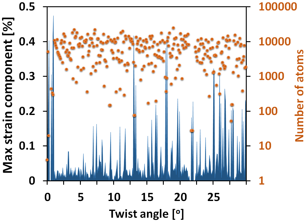
Figure 3: Absolute value of the maximum strain tensor component and number of atoms are presented for the supercells of bilayer graphene as a function of the twist angle. All supercells are generated using the developed software with resolution angle, $\Delta\theta=0.1^{\circ}$ up to $30^{\circ}$ and an $L_{\max}(A)\leq$ 20 parameter. For clarity, only the results with maximum strain component $\leq$ 0.5 $\%$ are presented. Visible dips in the blue bar plot correspond to configurations with moiré patterns. Note that there are many twist angles for which the number of atoms is in the hundreds.

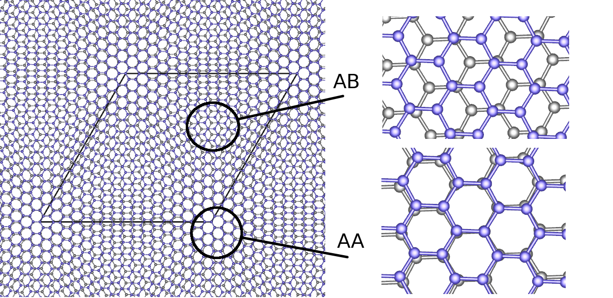
Figure 4: The moiré pattern forms on the bilayer graphene with a relative rotation angle (twist angle) between the layers equal to $\theta=6^{\circ}$. A unit cell determined by the software supercell-core is marked in blue and contains 364 atoms. Various local stacking configurations are clearly visible. AA and AB stackings are shown in zoom on the right side of the picture. Grey and violet points indicate the carbon atoms from the bottom and top layers, respectively.

Table 1: Structural information corresponding to bilayer graphene supercells generated by supercell-core software. The results are presented for the optimal supercells (small system size and nearly unstrained layers) and for particular twist angles between the graphene layers. The supercells of the bilayer graphene have been generated with twist angle resolution 0.1 ^∘, and $L_{\max}(A)\leq 20$ parameters. Note, that the supercell vectors can be calculated from $\vec{c_{1}}=m_{11}\vec{a_{1}}+m_{21}\vec{a_{2}}$ and $\vec{c_{2}}=m_{12}\vec{a_{1}}+m_{22}\vec{a_{2}}$ or from 2D rotation matrix and $n_{ij}$ parameters (see Eq. 1). The $m_{ij}$, $n_{ij}$, $\varepsilon_{ij}$ matrices are taken from log files. Only maximal strain tensor component is presented.

. Twist angle $\theta[^{\circ}]$ substrate layer (A) $M=(m_{ij})$ $\in\mathbb{Z}^{2x2}$ top layer (B) $N=(n_{ij})$ $\in\mathbb{Z}^{2x2}$ supercell size [Ų] $|\vec{c}_{1}|\times|\vec{c}_{2}|\times\sin(\measuredangle(\mathbf{c}_{1},\mathbf{c}_{2}))$ max. strain component (B₁) $\varepsilon_{ji}=(\varepsilon_{ij})^{T}$ supercell no. atoms 1.1 $\begin{pmatrix}30&60\\ -60&-29\end{pmatrix}$ $\begin{pmatrix}29&60\\ -60&-30\end{pmatrix}$ $127.8$ Å$\times 127.8$Å$\times\sin(61.1^{\circ})$ $\varepsilon_{xx}=\varepsilon_{yy}=0.027\%$ 10920 2.0 $\begin{pmatrix}50&33\\ -49&-16\end{pmatrix}$ $\begin{pmatrix}49&33\\ -50&-17\end{pmatrix}$ 121.8Å$\times$ 70.3Å$\times\sin(30^{\circ})$ $\varepsilon_{xy}=-0.01\%,\varepsilon_{yx}=0.01\%$ 3268 3.9 $\begin{pmatrix}9&17\\ -17&-8\end{pmatrix}$ $\begin{pmatrix}8&17\\ -17&-9\end{pmatrix}$ 36.2Å$\times$ 36.2Å$\times\sin(60^{\circ})$ $\varepsilon_{xy}=0.019\%,\varepsilon_{yx}=-0.019\%$ 868 6.0 $\begin{pmatrix}12&37\\ 21&57\end{pmatrix}$ $\begin{pmatrix}21&62\\ 12&31\end{pmatrix}$ 130.7Å$\times$ 107.5Å$\times\sin(1.9^{\circ})$ $\varepsilon_{xy}=-0.019\%,\varepsilon_{yx}=0.019\%$ 364 17.9 $\begin{pmatrix}12&37\\ 21&57\end{pmatrix}$ $\begin{pmatrix}21&62\\ 12&31\end{pmatrix}$ 71.2Å$\times$ 201.7Å$\times\sin(1.9^{\circ})$ $\varepsilon_{yx}=-0.006\%$ 372 21.8 $\begin{pmatrix}59&55\\ 13&12\end{pmatrix}$ $\begin{pmatrix}73&68\\ -16&-15\end{pmatrix}$ 163.5Å$\times$ 152.2Å$\times\sin(0.1^{\circ})$ $\varepsilon_{yx}=-0.025\%$ 28 27.8 $\begin{pmatrix}9&11\\ 42&47\end{pmatrix}$ $\begin{pmatrix}33&38\\ 21&23\end{pmatrix}$ 116Å$\times$ 131.2Å$\times\sin(0.8^{\circ})$ $\varepsilon_{xy}=-0.008\%$ 156 29.4 $\begin{pmatrix}19&49\\ -14&-31\end{pmatrix}$ $\begin{pmatrix}14&39\\ -19&-46\end{pmatrix}$ 42Å$\times$ 105.6Å$\times\sin(6.6^{\circ})$ $\varepsilon_{yx}=-0.028\%$ 388

Here we examine the construction of the supercell of bilayer graphene, which is a prototypical example of a bilayer system. For this reason, we use a two-atom unit cell of graphene with lattice vectors, $\vec{a}_{1}=(\frac{\sqrt{3}a}{2},\frac{-a}{2})$ and $\vec{a}_{2}=(\frac{\sqrt{3}a}{2},\frac{a}{2})$, assumed for both layers, where $a=2.46$ Åis a lattice constant of graphene. One of the graphene layers can be rotated with respect to the other by a relative angle, $\theta$ (twist angle). Supposing we want to find the twist angles that lead to the appearance of moiré patterns, we can use the Heterostructure.opt method from the code, and set the algorithm parameter to moire. It is also recommended to increase the value of the $L_{max}(A)$ (e.g., max_el to 20 or 50) in order to catch patterns that are only visible at long distance, and to use a small step for the values of $\theta$ (e.g., 0.025^∘). Then, the user can apply the log functionality to assess which angles are most promising (for details see section III).

In this example we set max$\_$el to 20 and the range for the twist angle as $\theta\in(0^{\circ},30^{\circ})$, with the step equal to 0.1^∘. The optimal supercells were found by applying these parameters, and the maximum strain tensor components of these supercells are presented in Fig. 3. Particular angles exist when the supercells are small (tens to hundreds of atoms) and have low strain values ($<0.03\%$). Some of the lowest-strain angles are collected in Table 1. In the case where two identical layers with a twist angle equal to $0^{\circ}$ are considered, the strain tensor is exactly zero, and the generated supercell is identical to the primary cell. Because of this obvious result, we do not include this case in Table 1. Note that the lattice mismatch is commonly calculated as the difference between the lattice constants, even for rotated layers with strain distributions that are different from those determined by this simple approximation. Therefore, supercells resulting from construction of such twisted layers are assumed to exhibit low strain values, although, in fact, the strain components (e.g., shear strains) can be substantial, and can influence the material’s electronic properties. The number of atoms in the substrate layer can be calculated using the equation, $det(M)\,\times N_{at}$, where $N_{at}$ is the number of atoms in primary cell, and M is equal to $M=(m_{ij})$. The number of atoms in other layers can be calculated in an analogous manner.

The results (Table 1) demonstrate that, for small twist angles, the size of the supercell is large and the number of atoms is high, whereas for large twist angles, the situation is reversed. These results confirm a well-known fact observed for twisted bilayer structures where the relevant length scale is on the order of $1/\theta$ Trambly de Laissardière, Mayou, and Magaud (2010). In particular, for small twist angles such as $1.1^{\circ}$ or $2^{\circ}$, the periodicity becomes large enough that it cannot be handled as lattice inputs for DFT codes. However, other potential approaches, such as tight binding methods (TB) Pyt (2020), can be used instead. Moreover, our supercell-core software successfully identifies the angles that have been reported previously based on STM experiments, specifically the $21.8\%$ Cisternas, Flores, and Vargas (2008) and $1.1\%$ Cao et al. (2018b) for bilayer systems. In addition, we present the visualisation of the optimal supercell generated for the twist angle of $6^{\circ}$ as shown in Fig. 4, where the moiré pattern is clearly visible along with various stacking configurations. The different stacking configurations of the bilayer graphene and theirs crucial impact on the electronic properties have been highlighted in many papers so far (see i.e. Ref.Birowska, Milowska, and Majewski (2011)), however, for a twisted layers many stacking configurations are automatically included within one supercell (see e.g. Fig. 4).

Table 2: Structural information corresponding to the optimal supercells generated by supercell-core software for the trilayer systems: trilayer graphene (TG) and hexagonal boron nitride/graphene/phosphorene (hBN/G/P). The supercells of the trilayer graphene have been generated with twist angle resolution equl to 0.1 ^∘, and $L_{\max}(A)\leq 80$. Only maximal strain tensor component is presented. The twist angles $\theta_{1}$, $\theta_{2}$ correspond to relative rotation of the graphene and phosphorene layers in respect to the hBN layer, respectively. For the clarity of presentation, only one of the maximal strain components is presented, however, in some of the cases presented here the $|\varepsilon_{xy}|=|\varepsilon_{yx}|$ or $|\varepsilon_{xx}|=|\varepsilon_{yy}|$.

System $L_{max}(A)$	Twist angles $\theta_{1}[^{\circ}],\theta_{2}[^{\circ}]$	bottom layer (A) $M=(m_{ij})$ $\in\mathbb{Z}^{2x2}$	middle layer (B1) $N=(n_{ij})$ $\in\mathbb{Z}^{2x2}$	top layer (B2) $N^{\prime}=(n^{\prime}_{ij})$ $\in\mathbb{Z}^{2x2}$	supercell size [$\AA^{2}$] $|\vec{c}_{1}|\times|\vec{c}_{2}|\times\sin(\measuredangle(\mathbf{c}_{1},\mathbf{c}_{2}))$	max. strain component layer B1; layer B2 ($\%$)	No. atoms
TG	$0,21.8$	$\begin{pmatrix}12&19\\ 3&3\end{pmatrix}$	$\begin{pmatrix}12&19\\ 3&3\end{pmatrix}$	$\begin{pmatrix}15&23\\ -3&-6\end{pmatrix}$	$33.8$Å$\times 50.8$Å$\times Sin(3.7^{\circ})$	0$\%$; $\varepsilon_{yx}=-0.005\%$	126
TG	$21.8,17.9$	$\begin{pmatrix}19&16\\ 10&-3\end{pmatrix}$	$\begin{pmatrix}26&17\\ -1&-9\end{pmatrix}$	$\begin{pmatrix}25&17\\ 1&-8\end{pmatrix}$	62.8Å$\times$ 36.2Å$\times Sin(30^{\circ})$	$\varepsilon_{yx}=-0.03\%$; $\varepsilon_{yx}=-0.005\%$	1302
TG	$6.0,27.9$	$\begin{pmatrix}17&11\\ -16&-5\end{pmatrix}$	$\begin{pmatrix}16&11\\ -17&-6\end{pmatrix}$	$\begin{pmatrix}11&10\\ -19&-9\end{pmatrix}$	40.6Å$\times$ 23.5Å$\times Sin(30^{\circ})$	$\varepsilon_{xy}=-0.019\%$; $\varepsilon_{yx}=-0.2\%$	546
hBN/G/P $L_{max}(A)\leq 10$	$6.7,0.8$	$\begin{pmatrix}4&6\\ -10&3\end{pmatrix}$	$\begin{pmatrix}3&7\\ -10&2\end{pmatrix}$	$\begin{pmatrix}-4&6\\ -4&-1\end{pmatrix}$	21.8Å$\times$ 19.9Å$\times Sin(115.7^{\circ})$	$\varepsilon_{xx}$=1.7$\%$; $\varepsilon_{yx}$=-1.9$\%$	403
hBN/G/P $L_{max}(A)\leq 10$	$10.9,29.9$	$\begin{pmatrix}6&6\\ -3&6\end{pmatrix}$	$\begin{pmatrix}6&8\\ -4&4\end{pmatrix}$	$\begin{pmatrix}0&7\\ -3&-3\end{pmatrix}$	13Å$\times$ 26Å$\times Sin(60^{\circ})$	$\varepsilon_{xx}$=0.11$\%$; $\varepsilon_{xy}$=-1.31$\%$	302
hBN/G/P $L_{max}(A)\leq 10$	$11.5,29.8$	$\begin{pmatrix}8&6\\ 9&-3\end{pmatrix}$	$\begin{pmatrix}11&6\\ 6&-4\end{pmatrix}$	$\begin{pmatrix}10&0\\ -4&-3\end{pmatrix}$	36.9Å$\times$ 13 Å$\times Sin(62^{\circ})$	$\varepsilon_{yy}$=-0.92$\%$; $\varepsilon_{yx}$=0.23$\%$	437
hBN/G/P $L_{max}(A)\leq 40$	$23.1,4.4$	$\begin{pmatrix}13&17\\ 17&-30\end{pmatrix}$	$\begin{pmatrix}23&6\\ 6&-29\end{pmatrix}$	$\begin{pmatrix}20&-10\\ 0&-13\end{pmatrix}$	65.2Å$\times$ 65.2 Å$\times Sin(120^{\circ})$	$\varepsilon_{xx}$=0.03$\%$; $\varepsilon_{yy}$=0.09$\%$	3802

IV.2 Trilayer systems: trilayer graphene (TG) and hBN/graphene/phosphorene

The natural extension of the bilayer system is to simply add another layer. In principle, our code allows the user to find the optimal supercell for $n$ layers exhibiting different types of symmetry.

Thus, in this example, we consider a trilayer van der Waals heterostructure consisting of hexagonal boron nitride, graphene, and phosphorene. This structure is significantly more complicated than the previous example. Although graphene and hBN share the same hexagonal symmetry and have similar lattice constants ($2.46$ Åand $2.52$Å, respectively), phosphorene has a rectangular lateral cell with lattice constants equal to $a=3.26$ Åand $b=4.35$ Å(optimised lattice constants obtained in LDA approximation for monolayer taken from Birowska et al. (2019), (see Fig. 6). These differences between the layers makes finding an optimal supercell more difficult.

The supercell-core software can be used to find the optimal configuration for this example with any combination of twist angles. The layer strains resulting from the generated supercells are presented in Fig. 5 as a function of two twist angles, $\theta_{1}$ and $\theta_{2}$. These angles ($\theta_{1}$, $\theta_{2}$) correspond to the relative rotation of the graphene (layer $B_{1}$) and phosporene (layer $B_{2}$) layers with respect to the hBN layer (layer A), respectively. The dark navy blue regions in Fig. 5 indicate the set of angles that correspond to supercells with relatively low strains. Table 2 provides the details regarding a few generated supercells that contain hundreds of atoms. The results clearly show that the strains in these supercells are relatively high. This is because we constrained the supercell size ($L_{max}(A)\leq 10$) so that the number of atoms is less than one thousand, while our system is composed of three incommensurate lattices. This is a fundamental problem of the system, and not a problem of the program. To find better supercells, one can loosen the constraints on the supercell size, although this introduces the risk of finding supercells that are too big for DFT calculations. In order to minimise the strain, it is recommended that the user increases the value of the $L_{max}(A)$ parameter. By increasing this parameter, one directly enlarges the supercell size considered, and thus, minimises the strain (see the last raw results in Table 2). Increasing the resolution of the twist angle may also help, in principle, but there is little chance that an optimal supercell would not be found with a resolution on the order of $0.1^{\circ}$.

In the Table 2, we also present selected supercells for trilayer graphene (TG). Note, that whenever one of the twist angles is zero, the results correspond to bilayer system (first raw in Table 2 for $\theta_{1}=0^{\circ}$, $\theta_{2}=21.8^{\circ}$). However, the software found different result than presented for bilayer system (see Table 1 for $\theta_{1}=21.8^{\circ}$). When supercell-core finds a true moiré pattern, any parallelogram with vertices on the repeated patterns’ nodes is a zero-strain supercell. The program should then find the smallest of such supercells. However, the calculated strain for each of those supercell is non-zero because of floating point errors. When choosing the optimal supercell, the program has some fixed tolerancy (epsilon) of the variation in the strain value but sometimes it happens to be too low to find the smallest supercell from a set of equally good supercells. A potential solution is to re-run the calculations for low-strain supercells with lower value of the $L_{max}(A)$ parameter.

Generally, for cases where $n>3$, it is difficult to obtain the commensurability condition for a relatively small system size, especially one with different types of layers that exhibit different symmetries.

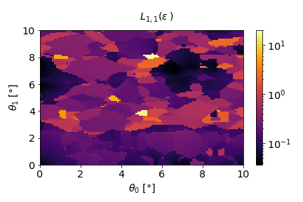
Figure 5: Strain distribution for an hBN/graphene/phosphorene heterostructure as a function of the twist angles, $\theta_{0}$ and $\theta_{1}$. For the clarity of the presentation, each angle is presented within the range ($0^{\circ},10^{\circ}$) and step size of $0.1^{\circ}$. The black colour indicates for the range of angles with the least amount of strain.

.

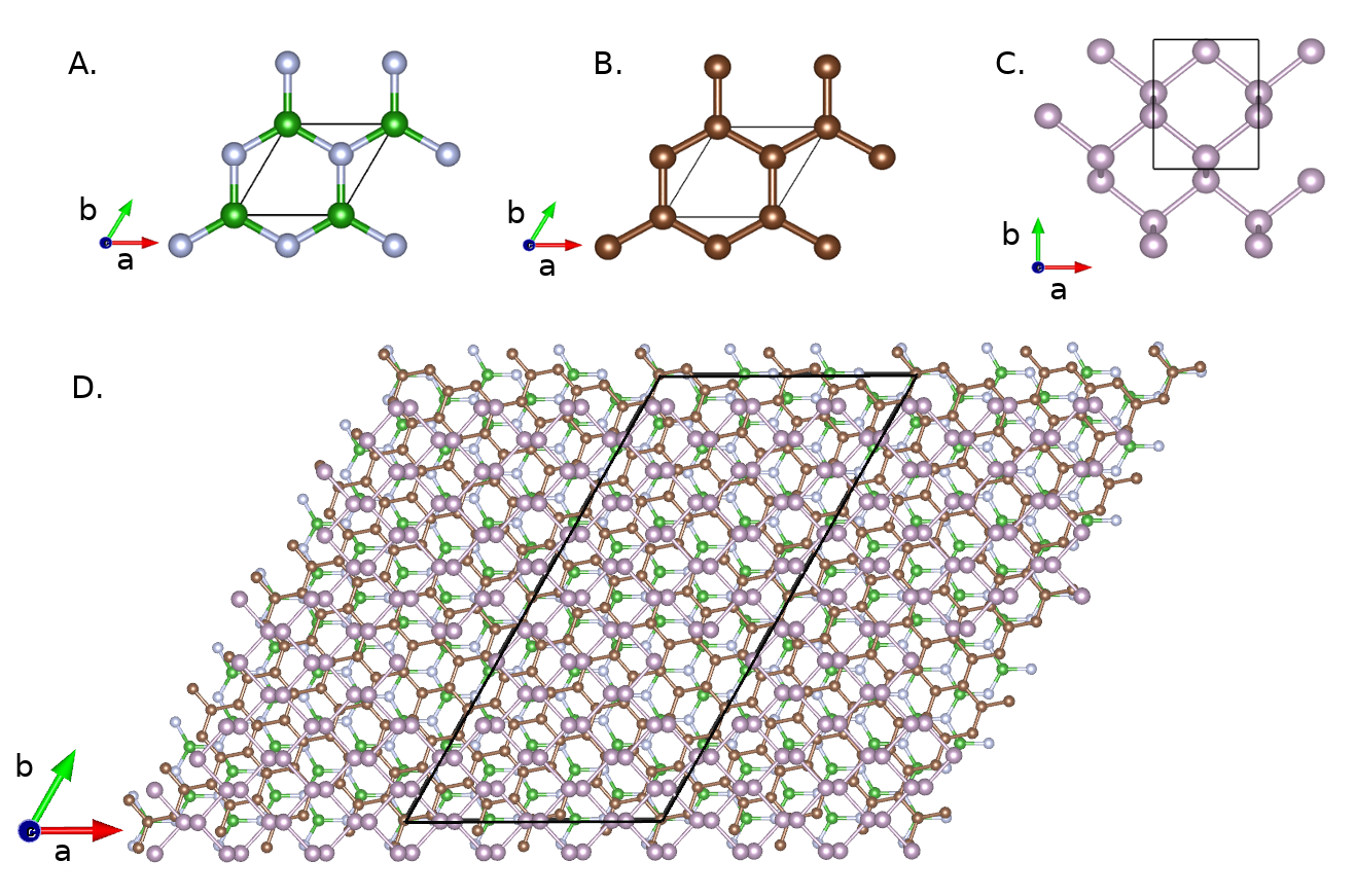
Figure 6: The primary cells of the A. hBN, B. graphene, and C. phoshorene layers used for constructing the optimal van der Waals trilayer hBN/G/P supercell and D. an example of an optimal supercell for a twisted trilayer hBN/G/P structure with twist angles equal to $\theta_{1}=10.9^{\circ}$ and $\theta_{2}=29.9^{\circ}$, corresponding to graphene and phosphorene rotations with respect to the hBN layer.

V CONCLUSIONS

In this report, we present the novel supercell-core software which has been developed to facilitate construction and analysis of vertically-aligned 2D layers. In principle, the code is designed to handle structures comprised of "n" different types of layers exhibiting different lateral symmetries. The developed software allows the user to find the optimal supercell, with the smallest number of atoms and lowest strains experienced by adjacent layers. The methodology is based on a commensurability condition, which implies long-range crystalline order in the sets of lattice planes that make up the van der Waals heterostructure. This condition is enforced by applying strain to the top layers of the structures. In the described approach, the bottom layer is always unstrained.

The software works with POSCAR files, and it is therefore compatible with the DFT software, VASP, and with the widely-used visualisation software, VESTA. In addition, there are two algorithms that are implemented, namely Direct and Fast. The former spans all possible configurations from which the supercells can be constructed, while the latter is more efficient and designed to search for unstrained configurations (e.g., those exhibiting moiré patterns). The former is more hefty and resource-intensive, while the latter is a more efficient algorithm.

Depending on the user’s requirements, the developed software also enables construction of the optimal supercells based on the twist angle(s) between the layers. It also allows users to study strained supercells in order to examine the impact of the strain distribution on the various properties of van der Waals heterostructures. Both types of results can be used as structural inputs for further calculations based on an ab initio approach (using DFT software, such as VASP, Quantum Espresso, or SIESTA). Particularly for cases of large supercells containing thousands of atoms, the results provided by our software can be used as structural inputs for software based on tight binding methods.

References

- Cisternas, Flores, and Vargas (2008) E. Cisternas, M. Flores, and P. Vargas, “Superstructures in arrays of rotated graphene layers: Electronic structure calculations,” Phys. Rev. B 78, 125406 (2008).
- Ohta et al. (2012) T. Ohta, J. T. Robinson, P. J. Feibelman, A. Bostwick, E. Rotenberg, and T. E. Beechem, “Evidence for interlayer coupling and moiré periodic potentials in twisted bilayer graphene,” Phys. Rev. Lett. 109, 186807 (2012).
- Hunt et al. (2013) B. Hunt, J. D. Sanchez-Yamagishi, A. F. Young, M. Yankowitz, B. J. LeRoy, K. Watanabe, T. Taniguchi, P. Moon, M. Koshino, P. Jarillo-Herrero, and R. C. Ashoori, “Massive dirac fermions and hofstadter butterfly in a van der waals heterostructure,” Science 340, 1427–1430 (2013), https://science.sciencemag.org/content/340/6139/1427.full.pdf .
- Cao et al. (2018a) Y. Cao, V. Fatemi, A. Demir, S. Fang, S. L. Tomarken, J. Y. Luo, J. D. Sanchez-Yamagishi, K. Watanabe, T. Taniguchi, E. Kaxiras, R. C. Ashoori, and P. Jarillo-Herrero, “Correlated insulator behaviour at half-filling in magic-angle graphene superlattices,” Nature 556, 80–84 (2018a).
- Zhu et al. (2020) Z. Zhu, P. Cazeaux, M. Luskin, and E. Kaxiras, “Modeling mechanical relaxation in incommensurate trilayer van der waals heterostructures,” Phys. Rev. B 101, 224107 (2020).
- Kang et al. (2017) P. Kang, W.-T. Zhang, V. Michaud-Rioux, X.-H. Kong, C. Hu, G.-H. Yu, and H. Guo, “Moiré impurities in twisted bilayer black phosphorus: Effects on the carrier mobility,” Phys. Rev. B 96, 195406 (2017).
- Decker et al. (2011) R. Decker, Y. Wang, V. W. Brar, W. Regan, H.-Z. Tsai, Q. Wu, W. Gannett, A. Zettl, and M. F. Crommie, “Local electronic properties of graphene on a bn substrate via scanning tunneling microscopy,” Nano Letters 11, 2291–2295 (2011).
- Woods et al. (2014) C. R. Woods, L. Britnell, A. Eckmann, R. S. Ma, J. C. Lu, H. M. Guo, X. Lin, G. L. Yu, Y. Cao, R. . V. Gorbachev, A. V. Kretinin, J. Park, L. A. Ponomarenko, M. I. Katsnelson, Y. N. Gornostyrev, K. Watanabe, T. Taniguchi, C. Casiraghi, H.-J. Gao, A. K. Geim, and K. . S. Novoselov, “Commensurate-incommensurate transition in graphene on hexagonal boron nitride,” Nature Physics 10, 451–456 (2014).
- Kang et al. (2013) J. Kang, J. Li, S.-S. Li, J.-B. Xia, and L.-W. Wang, “Electronic structural moiré pattern effects on mos2/mose2 2d heterostructures,” Nano Letters 13, 5485–5490 (2013).
- Alexeev et al. (2019) E. M. Alexeev, D. A. Ruiz-Tijerina, M. Danovich, M. J. Hamer, D. J. Terry, P. K. Nayak, S. Ahn, S. Pak, J. Lee, J. I. Sohn, M. R. Molas, M. Koperski, K. Watanabe, T. Taniguchi, K. S. Novoselov, R. V. Gorbachev, H. S. Shin, V. I. Fal’ko, and A. I. Tartakovskii, “Resonantly hybridized excitons in moiré superlattices in van der waals heterostructures,” Nature 567, 81–86 (2019).
- Geim (2013) I. V. Geim, A. K.and Grigorieva, “Van der waals heterostructures,” Nature 499, 419–425 (2013).
- Kunstmann et al. (2018) J. Kunstmann, F. Mooshammer, P. Nagler, Rodolfo, A. Chaves, F. Stein, N. Paradiso, G. Plechinger, C. Strunk, C. Schüller, G. Seifert, D. R. Reichman, and T. Korn, “Momentum-space indirect interlayer excitons in transition-metal dichalcogenide van der waals heterostructures,” Nature Physics 14 (2018), 10.1038/s41567-018-0123-y.
- Cao et al. (2018b) Y. Cao, V. Fatemi, S. Fang, K. Watanabe, T. Taniguchi, E. Kaxiras, and P. Jarillo-Herrero, “Unconventional superconductivity in magic-angle graphene superlattices,” Nature 556, 43–50 (2018b).
- Birowska et al. (2019) M. Birowska, J. Urban, M. Baranowski, D. K. Maude, P. Plochocka, and N. G. Szwacki, “The impact of hexagonal boron nitride encapsulation on the structural and vibrational properties of few layer black phosphorus,” Nanotechnology 30, 195201 (2019).
- Carr et al. (2017) S. Carr, D. Massatt, S. Fang, P. Cazeaux, M. Luskin, and E. Kaxiras, “Twistronics: Manipulating the electronic properties of two-dimensional layered structures through their twist angle,” Phys. Rev. B 95, 075420 (2017).
- Bukharaev et al. (2018) A. A. Bukharaev, A. K. Zvezdin, A. P. Pyatakov, and Y. K. Fetisov, “Straintronics: a new trend in micro- and nanoelectronics and materials science,” Physics-Uspekhi 61, 1175–1212 (2018).
- Hu, Zhou, and Dong (2017) T. Hu, J. Zhou, and J. Dong, “Strain induced new phase and indirect–direct band gap transition of monolayer inse,” Phys. Chem. Chem. Phys. 19, 21722–21728 (2017).
- Tamleh, Rezaei, and Jalilian (2018) S. Tamleh, G. Rezaei, and J. Jalilian, “Stress and strain effects on the electronic structure and optical properties of scn monolayer,” Physics Letters A 382, 339 – 345 (2018).
- Milowska, Birowska, and Majewski (2011) K. Milowska, M. Birowska, and J. A. Majewski, “Mechanical, electrical, and magnetic properties of functionalized carbon nanotubes,” AIP Conference Proceedings 1399, 827–828 (2011).
- Xue et al. (2011) J. Xue, J. Sanchez-Yamagishi, D. Bulmash, P. Jacquod, A. Deshpande, K. Watanabe, T. Taniguchi, P. Jarillo-Herrero, and B. J. LeRoy, “Scanning tunnelling microscopy and spectroscopy of ultra-flat graphene on hexagonal boron nitride,” Nature Materials 10, 282–285 (2011).
- Kresse and Müller (1996) G. Kresse and J. F. Müller, “Efficiency of ab-initio total energy calculations for metals and semiconductors using a plane-wave basis set,” Computational Materials Science 6, 15 – 50 (1996).
- Kresse and Hafner (1993) G. Kresse and J. Hafner, “Ab initio,” Phys. Rev. B 47, 558–561 (1993).
- Giannozzi and Stefano (2009) P. Giannozzi and B. Stefano, “Quantum espresso: a modular and open-source software project for quantum simulations of materials,” Journal of Physics: Condensed Matter 21, 395502 (2009).
- Soler et al. (2002) J. M. Soler, E. Artacho, J. D. Gale, A. García, J. Junquera, P. Ordejón, and D. Sánchez-Portal, “The SIESTA method forab initioorder-nmaterials simulation,” Journal of Physics: Condensed Matter 14, 2745–2779 (2002).
- Momma and Izumi (2008) K. Momma and F. Izumi, “VESTA: a three-dimensional visualization system for electronic and structural analysis,” Journal of Applied Crystallography 41, 653–658 (2008).
- Smidstrup et al. (2020) S. Smidstrup, T. Markussen, P. Vancraeyveld, J. Wellendorff, J. Schneider, T. Gunst, B. Verstichel, D. Stradi, P. A. Khomyakov, U. G. Vej-Hansen, et al., “Quantumatk: An integrated platform of electronic and atomic-scale modelling tools,” J. Phys: Condens. Matter 32, 015901 (2020).
- Wolf and Yip (1992) D. Wolf and S. Yip, Materials Interfaces. Atomic-level structure and properties, 1st ed. (Chapman & Hall, 1992).
- Virtanen et al. (2020) P. Virtanen, R. Gommers, T. E. Oliphant, M. Haberland, T. Reddy, D. Cournapeau, E. Burovski, P. Peterson, W. Weckesser, J. Bright, S. J. van der Walt, M. Brett, J. Wilson, K. Jarrod Millman, N. Mayorov, A. R. J. Nelson, E. Jones, R. Kern, E. Larson, C. Carey, İ. Polat, Y. Feng, E. W. Moore, J. Vand erPlas, D. Laxalde, J. Perktold, R. Cimrman, I. Henriksen, E. A. Quintero, C. R. Harris, A. M. Archibald, A. H. Ribeiro, F. Pedregosa, P. van Mulbregt, and S. . . Contributors, “SciPy 1.0: Fundamental Algorithms for Scientific Computing in Python,” Nature Methods 17, 261–272 (2020).
- pandas development team (2020) T. pandas development team, “pandas-dev/pandas: Pandas,” (2020).
- git (2020) "https://github.com/tnecio/supercell-core" (2020), accessed 2020-03-11.
- Trambly de Laissardière, Mayou, and Magaud (2010) G. Trambly de Laissardière, D. Mayou, and L. Magaud, “Localization of dirac electrons in rotated graphene bilayers,” Nano Letters 10, 804–808 (2010).
- Pyt (2020) "https://www.physics.rutgers.edu/pythtb/index.html" (2020), python Tight Binding (PythTB).
- Birowska, Milowska, and Majewski (2011) M. Birowska, K. Milowska, and J. A. Majewski, “Van Der Waals Density Functionals for Graphene Layers and Graphite,” Acta Physica Polonica A 120, 845–848 (2011).