Galactic extinction laws: II. Hidden in plain sight, a new interstellar absorption band at 7700 Å broader than any known DIB

Abstract

We have detected a broad interstellar absorption band centred close to 7700 Å and with a FWHM of 176.6$\pm$3.9 Å. This is the first such absorption band detected in the optical range and is significantly wider than the numerous diffuse interstellar bands (DIBs). It remained undiscovered until now because it is partially hidden behind the A telluric band produced by O₂. The band was discovered using STIS@HST spectra and later detected in a large sample of stars of diverse type (OB stars, BA supergiants, red giants) using further STIS and ground-based spectroscopy. The EW of the band is measured and compared with our extinction and K i $\lambda\lambda$7667.021,7701.093 measurements for the same sample. The carrier is ubiquitous in the diffuse and translucent Galactic ISM but is depleted in the environment around OB stars. In particular, it appears to be absent or nearly so in sightlines rich in molecular carbon. This behaviour is similar to that of the $\sigma$-type DIBs, which originate in the low/intermediate-density UV-exposed ISM but are depleted in the high-density UV-shielded molecular clouds. We also present an update on our previous work on the relationship between $E(4405-5495)$ and $R_{5495}$ and incorporate our results into a general model of the ISM.

1 Introduction

 The ISM imprints a large number of absorption lines in the optical range of stellar spectra. A few lines are well identified and their origin ascribed to atomic (e.g. Na i $\lambda\lambda$5891.583,5897.558) or molecular (e.g. CH $\lambda$4301.523) species but many of them are grouped under the term “diffuse interstellar bands” (DIBs) and their origin is debated, with just a few of them having had their carriers identified (Campbell et al., 2015; Cordiner et al., 2019). DIBs were discovered almost one century ago by Heger (1922) and the “diffuse” in the name refers to their larger intrinsic widths compared to atomic and molecular lines. They are typically divided into narrow (FWHM around 1 Å) and broad (FWHM from several Å up to 40 Å, e.g. Maíz Apellániz et al. 2015).

In the UV the situation is different, with many atomic ISM lines but no confirmed DIBs (Seab & Snow, 1985; Clayton et al., 2003), and the most significant absorption structure is the broad 2175 Å absorption band, which is much wider and stronger than any optical DIB (Bless & Savage, 1970; Savage, 1975). In the near infrared no broad absorption bands have been reported (but a few weak DIBs have) and in the mid infrared several broad absorption bands are seen and have been ascribed to silicates, H₂O, CO, CO₂, and aliphates (Fritz et al. 2011 and references therein).

In the optical range no clearly defined absorption bands have been reported until now but several very broad band structures have been detected with sizes of $\sim$1000 Å and larger (Whitford, 1958; Whiteoak, 1966; York, 1971; Massa et al., 2020), sometimes qualifying them as “knees” in the extinction law. As most previous families of extinction laws (e.g. Cardelli et al. 1989; Fitzpatrick 1999; Maíz Apellániz et al. 2014) are based on broad-band photometric data, those structures have been included to some extent in their analysis. However, Cardelli et al. (1989) used a polynomial interpolation in wavelength using as reference the Johnson filters and this led to artificial structures and incorrect results when using Strömgren photometry. The issue was addressed by Maíz Apellániz et al. (2014) by switching to spline interpolation.

This is the second paper of a series on Galactic extinction laws (but as Maíz Apellániz & Barbá 2018 is extensively cited in the text, it will be referred to as paper 0) that plans to cover the UV-optical-IR ranges. In paper I (Maíz Apellániz et al., 2020) we analysed the behaviour of extinction laws in the NIR using 2MASS data. Here we report the discovery of the first optical broad (FWHM $>$ 100 Å, broader than broad DIBs, see above) absorption band, centred at 7700 Å. We start describing the discovery of the new absorption band, then discuss the methods used to measure it, continue with our results and analysis, and finish with a summary and future plans. As the 7400–8000 Å wavelength range has been seldom explored spectroscopically relative to other parts of the optical spectrum, we include two appendices with the ISM and stellar lines that we have found in the data.

2 How did we find the new absorption band?

 Our first encounter with the new absorption band took place when preparing the spectral library for Maíz Apellániz & Weiler (2018). In that paper we produced a new photometric calibration for Gaia DR2 that was needed because of the presence of small colour terms when one compared the existing calibrations with good-quality spectrophotometry. Existing libraries that had been used for previous calibrations such as NGSL (Maíz Apellániz, 2017) had different issues so we built a new stellar library combining Hubble Space Telescope (HST) Space Telescope Imaging Spectrograph (STIS) G430L+G750L wide-slit low-resolution spectroscopy from different sources, mostly CALSPEC (Bohlin et al., 2019), HOTSTAR (Khan & Worthey, 2018), and the Massa library (Massa et al., 2020). When analysing the new spectral library, we noticed a broad absorption band close to 7700 Å in the spectra of extinguished OB stars. The intensity of the band was correlated with the amount of extinction and was much broader than any of the DIBs analysed in that region or indeed any DIBs (see e.g. Jenniskens & Desert 1994; Hobbs et al. 2008, 2009; Maíz Apellániz et al. 2015).

The Maíz Apellániz & Weiler (2018) stellar library includes only stars with weak extinction ($\mbox{$E(4405-5495)$}\lesssim 1$, see Maíz Apellániz 2004, 2013a to understand why monochromatic quantities should be used to define the amount or type of extinction), so the absorption band was relatively weak in those stars. We have recently started HST GO program 15 816 to extend the CALSPEC library to very red stars and in that way improve the Gaia photometric calibration for objects with large $G_{\rm BP}$$-$$G_{\rm RP}$, which are mostly high-extinction red giants (see paper I). In the first visit of that program we observed two such extinguished red giants (2MASS J16140974$-$5147147 and 2MASS J16141189$-$5146516) and we easily detected the absorption band there with the same central wavelength and similar FWHM, but clearly deeper. This confirmed the reality of the absorption band and its association with interstellar extinction.

Table 1: Spectrographs used, sample size observed with each, and associated EW₇₇₀₀ random uncertainties.

telesc. / aper. spectrograph spectral type # unc. observ. (m) resol. (Å) HST 2.4 STIS 800 long slit 26 0.4 LT 2.0 FRODOspec 2200 IFU 30 0.6 CAHA 3.5 CARMENES 95 000 échelle 26 0.6 La Silla 2.2 FEROS 46 000 échelle 55 1.8 NOT 2.5 FIES 25 000 échelle 49 2.0 67 000 échelle 7 2.0 Mercator 1.2 HERMES 85 000 échelle 44 0.9

Why was not this absorption band found earlier? The main reason is that its short-wavelength side is located in the deep O₂ telluric A band (7595–7715 Å), with the strongest absorption in the short-wavelength part of that range (a much weaker H₂O telluric band is present around 7900 Å). That is why the absorption band was identified in the few existing HST spectra rather than in the much more common ground-based data. Note that Massa et al. (2020) included this region in their study and that some of their stars overlap with our sample, clearly showing the absorption band but the authors missed it. It also appears in Fig. 7 of Callingham et al. (2020) but was not identified as an ISM absorption band there. Once we knew where to look it was not difficult to find the absorption band in ground-based data. For that purpose we used two types of spectra of OB stars and A supergiants. The first type is échelle data from four spectrographs (CARMENES@CAHA-3.5m, FEROS@La Silla 2.2 m, FIES@NOT, and HERMES@Mercator, see Table 1) that we have collected over the years for the LiLiMaRlin project (Library of Libraries of Massive-Star High-Resolution Spectra, Maíz Apellániz et al. 2019b) with the purposes of studying spectroscopic binaries (MONOS, Multiplicity Of Northern O-type Spectroscopic Systems, Maíz Apellániz et al. 2019c) and the intervening ISM (CollDIBs, Collection of DIBs, Maíz Apellániz 2015). We also analyzed data from two other spectrographs: CAFÉ@CAHA-2.2 m and UVES@VLT but ended up not using them. In the first case we discarded it because of the existence of several gaps between orders in the wavelength region of interest and in the second one because of the poor order stitching in most spectra. The second type of spectra was acquired with the dual-beam FRODOspec spectrograph at the Liverpool Telescope (LT) for the Galactic O-Star Spectroscopic Survey (GOSSS, Maíz Apellániz et al. 2011) at a spectral resolution of 2200 at 7700 Å. The band is seen in both the échelle and the single-order spectra, especially when one excludes the wavelength region where the telluric absorption is strongest. The comparison between the two types of spectra produced an insight into a possible additional reason why the absorption band had not been discovered earlier. Échelle spectrographs are commonly used nowadays due to their high dispersion, which in our case is useful because it allows us to more easily subtract the contribution from the telluric, stellar (see Appendix B), and ISM (e.g K i $\lambda\lambda$7667.021,7701.093) lines that are present in the data. However, the high-resolution comes with a problem: broad-wavelength structures such as the one we are interested in are dispersed in two or more orders and the blaze-function correction can introduce effects at the 1–2% level that can bias results or even mask the structure altogether. In this respect, single-order spectrographs such as FRODOspec have the advantage of permitting a more accurate spectral rectification at the expense of a lower spectral resolution. As explained in the next section, our combination of both techniques has allowed us to study the new absorption band in a large sample of stars.

3 Methods

 In the previous section we described how we discovered the new absorption band. Here we describe how we selected our sample and how we have measured the band. The measurement process takes a different (and more complicated) route because of the different properties of the spectroscopy we use (space- or ground-based; low, intermediate or high spectral resolution; single-order or échelle), the different types of stars present in the sample (mostly hot stars but also two red giants), and the need to take into account the different narrow lines present (telluric, stellar, and ISM).

3.1 Getting rid of those pesky absorption and emission lines

 Our spectra contain not only the absorption band we are interested in but also other ISM absorption, stellar absorption and emission, and (for ground-based data) telluric absorption lines. With respect to the first two types we provide two appendices where we list our results for them. Those results are not the main topic of this paper but undoubtedly are of interest for other pursuits, especially considering that this wavelength region has been studied in less detail than others in the optical.

We start with the telluric lines. First, we modified our pipelines for both LiLiMaRlin (high resolution) and LT (intermediate resolution) to rectify the spectra without using any points in the region around the absorption band. Both pipelines automatically fit O₂ and H₂O telluric absorption in this region using the Gardini et al. (2013) models and adjusting the spectral resolution, intensity, and velocity. As the O₂ lines are very deep, the central part of their cores can be difficult to be properly fit in the high-resolution data. However, as for many of our stars we have more than one epoch and as the telluric lines change in position with respect to the astrophysical ones throughout the year, in those cases we combine different observations of the same target selecting in each case the wavelength regions that are less affected by the telluric absorption. Nevertheless, the wavelength region with the highest telluric O₂ absorption (7595–7650 Å) cannot be properly corrected in most cases so we exclude it from our analysis.

With respect to the ISM lines there are several DIBs (see Appendix A) that can be ignored as they either fall outside the critical region of 7650–7750 Å where the absorption band is deeper or they are too weak to contribute significantly to our measurements. However, the K i $\lambda\lambda$7667.021,7701.093 doublet falls in the critical region and needs to be accounted for. To correct it, we have measured the two lines in the high resolution data and used the result to subtract Gaussian profiles of the proper equivalent width, velocity, and spectral resolution in the low- and intermediate-resolution spectra (note that the lines are unresolved in those data). In the high resolution data we simply interpolate between the adjacent wavelengths to eliminate the K i $\lambda\lambda$7667.021,7701.093 doublet.

Finally, different stellar lines are seen as a function of spectral type (see Appendix B). The most ubiquitous strong stellar line in our data is He ii $\lambda$7594.844, which appears in absorption for O stars of all subtypes and becomes stronger for the earlier subtypes. However, we can safely ignore it for most purposes and simply exclude it in our fitting of the line in the Gaia DR2 STIS sample, as it falls away from the critical 7650–7750 Å region. For the ground-based data most of the line is in any case overwhelmed by the head of the O₂ telluric A band. A similar case is the O i $\lambda\lambda\lambda$7774.083,7776.305,7777.527 triplet seen in absorption in the late-B and early-O supergiants in our sample, as we can also exclude that region from our fits for those stars. On the other hand, there are three lines seen in emission in early-to-mid O stars that fall in the critical region so for those targets we followed a process analogous to the one for the K i $\lambda\lambda$7667.021,7701.093 doublet to correct for their influence (but here fitting emission lines as opposed to absorption ones, see Appendix B for details).

3.2 Determination of the properties of the absorption band from the Gaia STIS samples

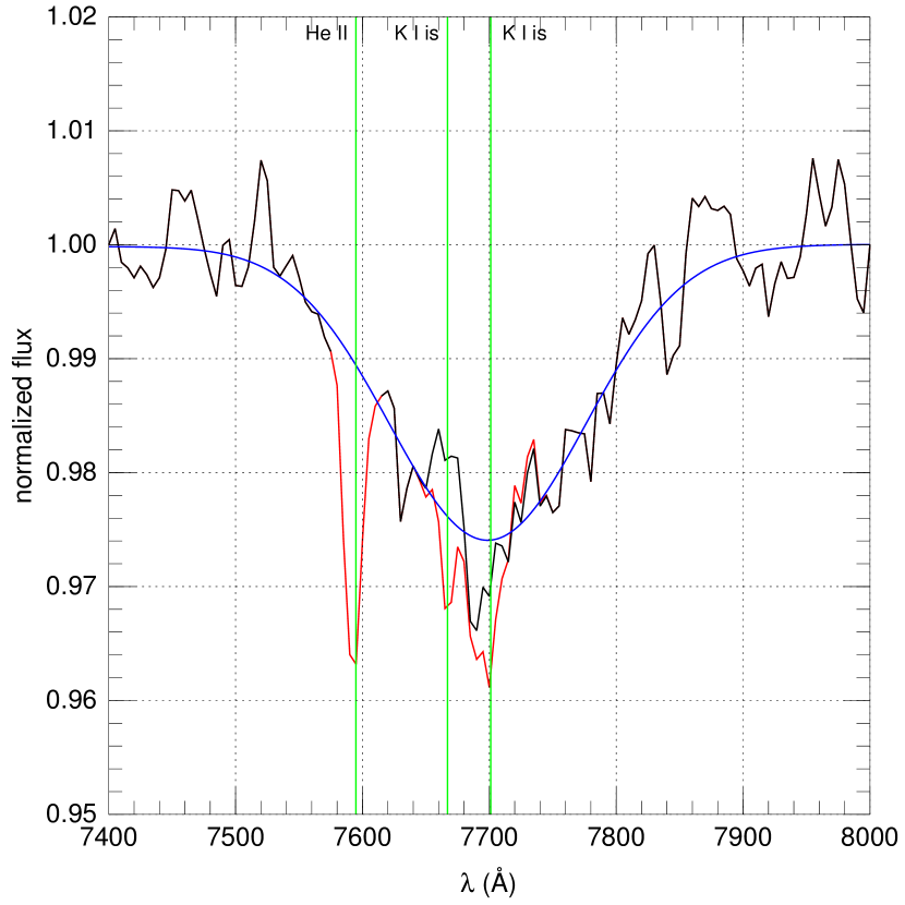
Figure 1: Combined weighted profile of the 7700 Å band generated from 24 O4–B1-type G750L STIS spectra. The black line is the profile itself, the red line is the profile without subtracting the absorption/emission lines and without blocking the He ii $\lambda$7594.844 line, the blue line is the fitted Gaussian, and the green lines mark the position of the three main absorption lines.

 We combined the STIS samples we used for our analysis of Gaia DR1 (Maíz Apellániz, 2017) and DR2 (Maíz Apellániz & Weiler, 2018) photometry, selecting the stars with O4–B1 spectral types from GOSSS, with good-quality NIR photometry, not affected by visual binarity, and for which we have good-quality high-resolution spectra. There are 24 such stars. For them we make an initial measurement of the absorption band by fitting an unrestricted Gaussian profile to each spectrum after (a) rectifying it, (b) correcting it for emission/absorption lines as described in the previous subsection, and (c) shifting it to an ISM velocity frame as defined by the K i $\lambda$7701.093 velocity (the latter effect being very small due to the low spectral resolution of the STIS data). Then, a combined profile is obtained by merging the 24 spectra weighed by their equivalent widths (Fig. 1). Finally, a Gaussian profile is fitted to the combined profile excluding the He ii $\lambda$7594.844 absorption line from the fit.

The Gaussian fit yields a central wavelength of 7699.2$\pm$1.3 Å (vacuum) and a FWHM of 176.6$\pm$3.9 Å, which we take as our preferred values for the absorption band. The fit is of good quality within the S/N, which is not very high (Fig. 2) because of the relatively short exposure times of the HST spectroscopy. We also fit a profile without subtracting the emission/absorption lines (still excluding the He ii $\lambda$7594.844 absorption line from the fit) and in that case we obtain a central wavelength of 7695.1$\pm$1.1 Å and a FWHM of 164.1$\pm$3.1 Å, indicating that the effect of such lines (especially K i $\lambda\lambda$7667.021,7701.093, as the emission lines are relatively weak in the STIS O4–B1 sample) introduces a significant bias if left uncorrected. The effect of not excluding the He ii $\lambda$7594.844 absorption line would be even greater, but in that case the profile would clearly deviate from a Gaussian. Therefore, from now on we refer to the absorption band by its approximate central wavelength of 7700 Å.

Once we determined the FWHM of the profile, we fit a Gaussian profile of fixed width (see above) to each of the stars in the STIS O4–B1 sample to measure their equivalent widths (EW₇₇₀₀, see below for the results). The main source of uncertainty for the EW in a relatively weak and broad absorption feature such as this one is the rectification of the spectrum. To determine it, we performed Monte Carlo simulations of the continuum around the line with the appropriate S/N and determined the scatter in the measured EW₇₇₀₀ after rectifying each simulation, arriving at values between 0.3 Å and 0.5 Å. Therefore, we adopt an uncertainty of 0.4 Å for the measurements of the STIS O4–B1 sample. See Fig. 2 for three sample spectra.

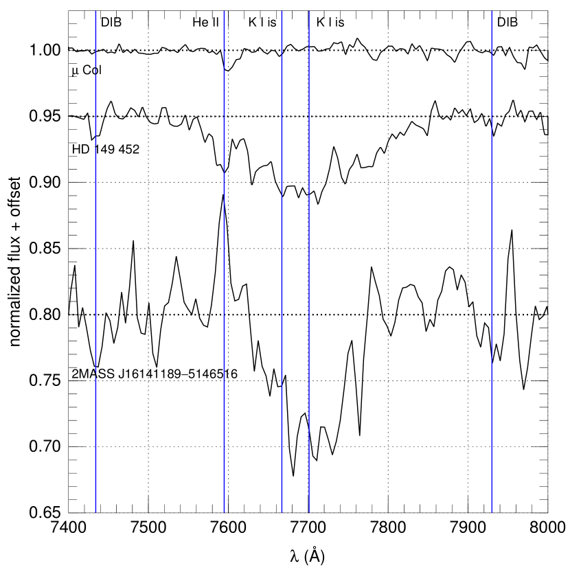
Figure 2: Three sample G750L STIS spectra sorted by EW₇₇₀₀ from non-detection to one of the red giants. The main stellar and ISM absorption lines have been left in place marked with blue vertical lines.

3.3 Extending the sample to the high extinction regime

 The O4–B1 STIS sample is relatively small and, more importantly, of low extinction (all objects have $\mbox{$E(4405-5495)$}<1$ mag). As we are studying an ISM absorption feature, we need to extend our extinction range to higher values to properly study its behaviour. As already mentioned, we have done this with the two high-extinction red giants observed with STIS and by extending our sample to 120 OBA stars with ground-based data and with a wide range of values of $E(4405-5495)$. The two red giants from HST GO program 15 816 had to be treated differently from the OB stars observed with STIS (note they were not used to determine the profile in the previous subsection). We first estimated their temperature by comparing their rectified spectra with models from the previously mentioned Maíz Apellániz (2013b) grid for red giants obtained from the MARCS models of Gustafsson et al. (2008) and obtained a value of 3800 K. As late-type stars have a multitude of absorption lines that cannot be seen at the low STIS resolution, we divided each spectra by that of the MARCS SED with the proper distance and extinction using the Maíz Apellániz et al. (2014) extinction laws (see below). For those two stars we also have to subtract the effect of the K i $\lambda\lambda$7667.021,7701.093 but we do not have high-resolution spectroscopy to do so. Therefore, we used the results from Appendix A to determine average EWs for K i $\lambda\lambda$7667.021,7701.093 for their extinctions and subtract the appropriate profiles in the STIS spectra. After doing that, we fit a Gaussian profile of fixed width as we previously did for the rest of the STIS sample and we obtain values of 14.0$\pm$1.3 Å for 2MASS J16140974$-$5147147 and 13.5$\pm$1.3 Å for 2MASS J16141189$-$5146516.

For the STIS sample we are limited by the relatively scarce sample available in the HST archive. For the ground-based data, on the other hand, we have a sample of over 1000 targets observed with FRODOspec and of 2000 targets in LiLiMaRlin to choose from. To build the sample we used several criteria:

• Good S/N (Fig. 4) and, if possible, observed with two or three telescopes for cross-calibration purposes.

• Inclusion of all stars in the STIS O4–B1 sample.

• Targets with multiple epochs are favoured to facilitate the elimination of telluric lines.

• Objects with different values of extinction are included but preference is given to those with high $E(4405-5495)$ or high $R_{5495}$ (Maíz Apellániz, 2013b), which are absent in the STIS O4–B1 sample.

• Most selected stars are of O spectral type but we have included some B stars that are of special interest as they have been previously used for ISM studies (e.g. Cyg OB2-12 and HT Sge) and one A supergiant (CE Cam).

As previously mentioned, in all ground-based spectra we first correct the telluric lines. Then, in the FRODOspec (intermediate resolution) spectra the stellar and ISM lines are corrected using Gaussian profiles and in the LiLiMaRlin (high resolution) the stellar lines are corrected in the same way and the K i $\lambda\lambda$7667.021,7701.093 doublet is interpolated from neighbour wavelengths. Finally, we fit a Gaussian profile of fixed width blocking regions with strong telluric lines and defects.

3.4 Cross-calibration of the data

 Before using the values of EW₇₇₀₀ band from the three different types of spectra in this paper (STIS long-slit low-resolution, FRODOspec IFU intermediate-resolution, and échelle high-resolution from different spectrographs) it is necessary to compare them to (a) identify and correct systematic biases between them and (b) properly characterize random uncertainties. In other words, to ensure that they are accurate and that we are using the right precision.

We have already determined that the random uncertainty of the EW₇₇₀₀ for the STIS O4–B1 sample is 0.4 Å. We also judge that there is no systematic bias in those measurements for two reasons: the high quality of the spectrophotometric calibration of STIS in absolute terms (Bohlin et al., 2019) and compared to Gaia DR2 (Maíz Apellániz & Weiler, 2018) and the fact that for the stars with negligible extinction we measure values of zero for EW₇₇₀₀.

For the rest of the spectrographs we first selected the sample in common between each one of them and the STIS O4–B1 sample and calculated the average and dispersion between the raw EW₇₇₀₀ for each spectrograph pair. We used the average to correct the systematic bias and the dispersion to estimate the random uncertainty of the measurements of each spectrograph (Table 1). We then compared the results from each spectrograph to verify the results. Table 1 indicates that the lowest uncertainties are those of LT (FRODOspec being a single-order spectrograph does not require order stitching) and, especially, CARMENES (a spectrograph of exquisite stability designed for planet hunting with extreme precision). Once the EW₇₇₀₀ from different sources are obtained in this way, the values for objects with multiple sources are combined using their weighted means (Table 2). Sample ground-based data are shown in Figs. 3 and 4.

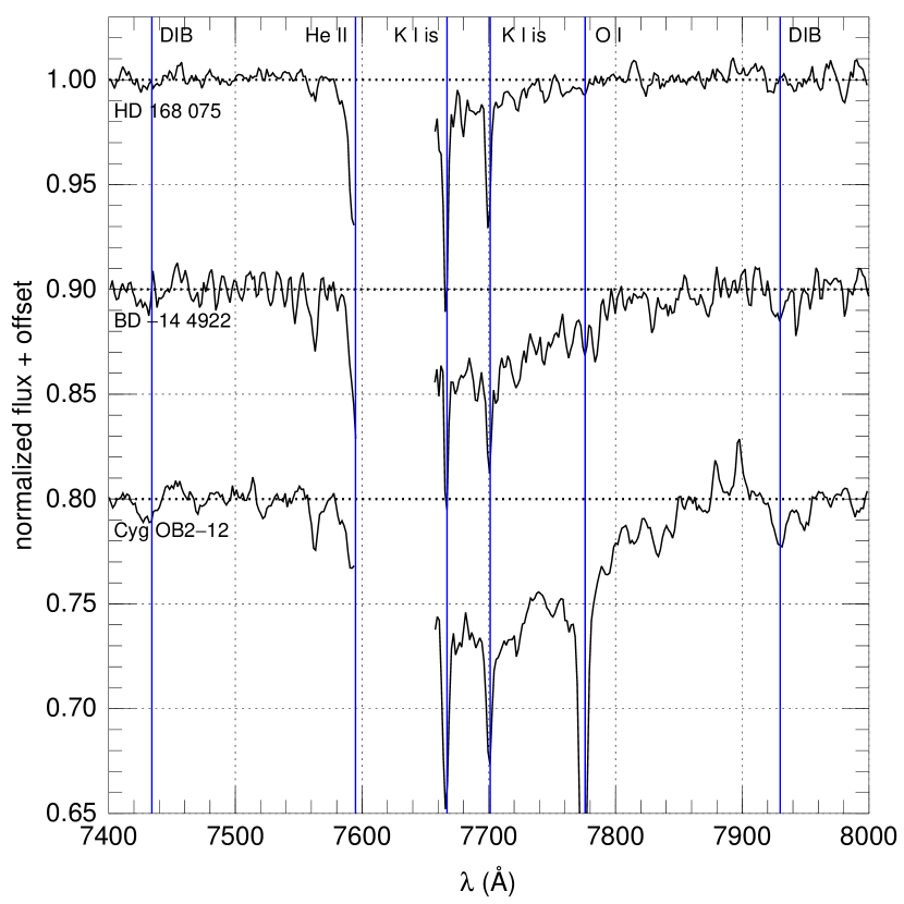
Figure 3: Three sample LT spectra sorted by EW₇₇₀₀. The main stellar and ISM absorption lines have been left in place marked with blue vertical lines but the wavelength region with the strongest O₂ telluric absorption has been eliminated.

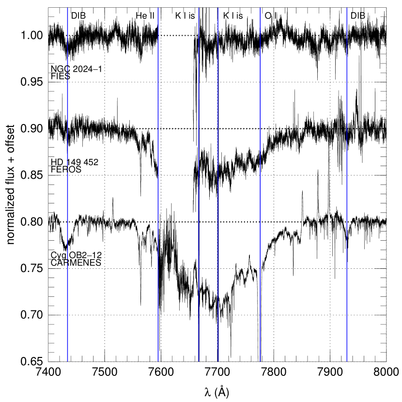
Figure 4: Three sample échelle spectra sorted by EW₇₇₀₀. The main stellar and ISM absorption lines have been left in place marked with blue vertical lines but the wavelength region with the strongest O₂ telluric absorption has been eliminated for the first two spectra. For the third spectrum we have maintained that region due to two exceptional circumstances: CARMENES is a highly stable spectrograph and the shown spectrum is a combination of 73 different epochs. As the telluric lines shift in wavelength with respect to the heliocentric frame of reference at different times of the year, we can combine the different epochs to minimize their effect even in a region with strong telluric absorption such as the O₂ A band.

Table 2: Results for the 7700 Å absorption band for OBA stars.

star code RA dec EW (J2000) (J2000) (Å) $\delta$ Ori Aa,Ab CFH 05:32:00.398 $-$00:17:56.69 0.8$\pm$ 0.5 $\mu$ Col SNH 05:45:59.895 $-$32:18:23.18 0.0$\pm$ 0.4 $\lambda$ Lep SH 05:19:34.525 $-$13:10:36.43 0.1$\pm$ 0.4 15 Mon Aa,Ab LCH 06:40:58.656 $+$09:53:44.71 0.3$\pm$ 0.4 $\rho$ Leo A,B SLH 10:32:48.671 $+$09:18:23.71 0.8$\pm$ 0.3 $\theta^{1}$ Ori Ca,Cb LCFNH 05:35:16.463 $-$05:23:23.18 1.1$\pm$ 0.4 $\sigma$ Ori Aa,Ab,B LCF 05:38:44.765 $-$02:36:00.25 1.8$\pm$ 0.4 HD 93 028 SF 10:43:15.340 $-$60:12:04.21 2.3$\pm$ 0.4 $\theta^{2}$ Ori A CFNH 05:35:22.900 $-$05:24:57.80 0.8$\pm$ 0.5 NU Ori SH 05:35:31.365 $-$05:16:02.60 4.4$\pm$ 0.4 $\sigma$ Sco Aa,Ab LFH 16:21:11.313 $-$25:35:34.09 4.5$\pm$ 0.5 $\lambda$ Ori A CFH 05:35:08.277 $+$09:56:02.96 1.2$\pm$ 0.5 HD 164 402 SLN 18:01:54.380 $-$22:46:49.06 2.8$\pm$ 0.3 HD 46 966 Aa,Ab SH 06:36:25.887 $+$06:04:59.47 0.6$\pm$ 0.4 HD 93 205 F 10:44:33.740 $-$59:44:15.46 0.0$\pm$ 1.8 9 Sgr A,B SFH 18:03:52.446 $-$24:21:38.64 2.3$\pm$ 0.4 $\alpha$ Cam SC 04:54:03.011 $+$66:20:33.58 1.4$\pm$ 0.3 $\zeta$ Oph FNH 16:37:09.530 $-$10:34:01.75 2.1$\pm$ 0.7 CPD $-$59 2591 SF 10:44:36.688 $-$59:47:29.63 4.6$\pm$ 0.4 HD 34 656 CH 05:20:43.080 $+$37:26:19.23 2.4$\pm$ 0.5 Herschel 36 LFN 18:03:40.333 $-$24:22:42.74 2.0$\pm$ 0.5 V662 Car F 10:45:36.318 $-$59:48:23.37 10.0$\pm$ 1.8 CE Cam LCH 03:29:54.746 $+$58:52:43.51 5.7$\pm$ 0.4 HD 93 162 F 10:44:10.389 $-$59:43:11.09 0.1$\pm$ 1.8 HD 192 639 SLNH 20:14:30.429 $+$37:21:13.83 5.2$\pm$ 0.3 HD 93 250 A,B SF 10:44:45.027 $-$59:33:54.67 2.6$\pm$ 0.4 BD $-$16 4826 N 18:21:02.231 $-$16:01:00.94 8.2$\pm$ 2.0 HD 46 150 SCF 06:31:55.519 $+$04:56:34.27 4.2$\pm$ 0.3 CPD $-$59 2626 A,B F 10:45:05.794 $-$59:45:19.60 1.0$\pm$ 1.8 HD 149 452 SF 16:37:10.514 $-$47:07:49.85 9.4$\pm$ 0.4 HD 93 129 Aa,Ab F 10:43:57.462 $-$59:32:51.27 1.1$\pm$ 1.8 HD 93 161 A F 10:44:08.840 $-$59:34:34.49 5.4$\pm$ 1.8 HDE 326 329 F 16:54:14.106 $-$41:50:08.48 5.1$\pm$ 1.8 HD 48 279 A SLF 06:42:40.548 $+$01:42:58.23 3.2$\pm$ 0.3 HDE 322 417 F 16:58:55.392 $-$40:14:33.34 3.1$\pm$ 1.8 AE Aur SCH 05:16:18.149 $+$34:18:44.33 3.0$\pm$ 0.3 CPD $-$47 2963 A,B F 08:57:54.620 $-$47:44:15.71 3.4$\pm$ 1.8 $\lambda$ Cep SLNH 22:11:30.584 $+$59:24:52.25 2.0$\pm$ 0.3 HD 199 216 SLH 20:53:52.404 $+$49:32:00.33 2.8$\pm$ 0.3 NGC 2024-1 CN 05:41:37.853 $-$01:54:36.48 2.0$\pm$ 0.6 ALS 15 210 F 10:44:13.199 $-$59:43:10.33 0.0$\pm$ 1.8 HD 46 223 CH 06:32:09.306 $+$04:49:24.73 4.0$\pm$ 0.5 HDE 319 702 F 17:20:50.610 $-$35:51:45.97 3.7$\pm$ 1.8 ALS 19 613 A CN 18:20:29.902 $-$16:10:44.33 15.8$\pm$ 0.6 Cyg OB2-11 N 20:34:08.513 $+$41:36:59.42 14.9$\pm$ 2.0 HDE 319 703 A F 17:19:46.156 $-$36:05:52.34 9.1$\pm$ 1.8 HT Sge LCFH 19:27:26.565 $+$18:17:45.19 10.3$\pm$ 0.4 ALS 2063 F 10:58:45.475 $-$61:10:43.01 6.8$\pm$ 1.8 Cyg OB2-1 A N 20:31:10.543 $+$41:31:53.47 14.8$\pm$ 2.0 Cyg OB2-15 N 20:32:27.666 $+$41:26:22.08 12.5$\pm$ 2.0 ALS 4962 FN 18:21:46.166 $-$21:06:04.42 7.4$\pm$ 1.3 Cyg OB2-20 N 20:31:49.665 $+$41:28:26.51 14.9$\pm$ 2.0 BD $+$36 4063 N 20:25:40.608 $+$37:22:27.07 5.6$\pm$ 2.0 ALS 19 693 F 17:25:29.167 $-$34:25:15.74 6.8$\pm$ 1.8 BD $-$13 4930 SLF 18:18:52.674 $-$13:49:42.60 5.6$\pm$ 0.3 HD 156 738 A,B F 17:20:52.656 $-$36:04:20.54 6.2$\pm$ 1.8 CPD $-$49 2322 F 09:15:52.787 $-$50:00:43.82 5.0$\pm$ 1.8 BD $-$14 5014 N 18:22:22.310 $-$14:37:08.46 6.8$\pm$ 2.0 W 40 OS 1a C 18:31:27.837 $-$02:05:23.66 3.3$\pm$ 0.6 NGC 1624-2 N 04:40:37.248 $+$50:27:40.96 7.6$\pm$ 2.0 Codes: S,STIS; L,FRODOspec; C, CARMENES;  Codes: F, FEROS; N, FIES; H, HERMES.

Table 2: (continued).

star code RA dec EW (J2000) (J2000) (Å) HD 207 198 SLCH 21:44:53.278 $+$62:27:38.04 2.0$\pm$ 0.3 BD $-$12 4979 CF 18:18:03.112 $-$12:14:34.28 10.0$\pm$ 0.6 Cyg OB2-B18 H 20:34:57.858 $+$41:43:54.22 13.5$\pm$ 0.9 BD $+$60 513 SN 02:34:02.530 $+$61:23:10.87 5.7$\pm$ 0.4 HD 217 086 SLNH 22:56:47.194 $+$62:43:37.60 5.2$\pm$ 0.3 Cyg OB2-4 B LN 20:32:13.117 $+$41:27:24.25 13.8$\pm$ 0.6 BD $-$14 4922 LN 18:11:58.104 $-$14:56:08.97 9.7$\pm$ 0.6 HDE 319 703 Ba,Bb F 17:19:45.050 $-$36:05:47.00 11.5$\pm$ 1.8 Tyc 8978-04440-1 F 12:11:18.531 $-$62:29:43.53 5.3$\pm$ 1.8 HD 168 076 A,B F 18:18:36.421 $-$13:48:02.38 3.7$\pm$ 1.8 HD 168 112 A,B LFN 18:18:40.868 $-$12:06:23.39 6.8$\pm$ 0.5 LS I $+$61 303 N 02:40:31.667 $+$61:13:45.53 5.0$\pm$ 2.0 LS III $+$46 12 NH 20:35:18.566 $+$46:50:02.90 4.9$\pm$ 0.8 HD 194 649 A,B LNH 20:25:22.124 $+$40:13:01.07 6.4$\pm$ 0.5 HDE 323 110 F 17:21:15.794 $-$37:59:09.58 9.2$\pm$ 1.8 BD $-$14 5040 N 18:25:38.896 $-$14:45:05.70 5.3$\pm$ 2.0 MY Ser Aa,Ab FN 18:18:05.895 $-$12:14:33.29 6.6$\pm$ 1.3 Cyg OB2-8 A NH 20:33:15.078 $+$41:18:50.51 10.6$\pm$ 0.8 BD $+$61 487 LN 02:50:13.632 $+$62:05:30.81 8.5$\pm$ 0.6 BD $-$11 4586 CF 18:18:03.344 $-$11:17:38.83 9.0$\pm$ 0.6 Cyg OB2-5 A,B LNH 20:32:22.422 $+$41:18:18.91 10.0$\pm$ 0.5 HD 168 075 SLCFN 18:18:36.043 $-$13:47:36.46 4.8$\pm$ 0.3 Tyc 7370-00460-1 FN 17:18:15.396 $-$34:00:05.94 12.7$\pm$ 1.3 Cyg OB2-7 NH 20:33:14.115 $+$41:20:21.86 8.2$\pm$ 0.8 V479 Sct FN 18:26:15.045 $-$14:50:54.33 4.7$\pm$ 1.3 BD $-$13 4923 LFN 18:18:32.732 $-$13:45:11.88 6.0$\pm$ 0.5 Sh 2-158 1 NH 23:13:34.435 $+$61:30:14.73 15.0$\pm$ 0.8 HD 166 734 LF 18:12:24.656 $-$10:43:53.04 6.5$\pm$ 0.6 BD $+$62 2078 N 22:25:33.579 $+$63:25:02.62 6.5$\pm$ 2.0 LS III $+$46 11 LNH 20:35:12.642 $+$46:51:12.12 6.1$\pm$ 0.5 ALS 18 748 F 17:19:04.436 $-$38:49:04.87 13.0$\pm$ 1.8 Pismis 24-1 A,B FH 17:24:43.502 $-$34:11:56.96 9.6$\pm$ 0.8 Cyg OB2-A11 NH 20:32:31.543 $+$41:14:08.21 14.8$\pm$ 0.8 Cyg X-1 CN 19:58:21.677 $+$35:12:05.81 5.0$\pm$ 0.6 BD $-$13 4929 F 18:18:45.857 $-$13:46:30.83 1.3$\pm$ 1.8 ALS 15 108 A,B H 20:33:23.460 $+$41:09:13.02 14.8$\pm$ 0.9 HD 15 570 SCH 02:32:49.422 $+$61:22:42.07 4.6$\pm$ 0.3 ALS 19 307 N 19:50:01.087 $+$26:29:34.36 15.5$\pm$ 2.0 Cyg OB2-3 A,B NH 20:31:37.509 $+$41:13:21.01 15.5$\pm$ 0.8 ALS 15 133 N 20:31:18.330 $+$41:21:21.66 19.7$\pm$ 2.0 Cyg OB2-73 N 20:34:21.930 $+$41:17:01.60 16.1$\pm$ 2.0 NGC 3603 HST-5 F 11:15:07.640 $-$61:15:17.56 11.0$\pm$ 1.8 Cyg OB2-22 A H 20:33:08.760 $+$41:13:18.62 13.1$\pm$ 0.9 Cyg OB2-B17 N 20:30:27.302 $+$41:13:25.31 12.5$\pm$ 2.0 THA 35-II-42 F 10:25:56.505 $-$57:48:43.50 7.4$\pm$ 1.8 ALS 15 131 N 20:33:02.922 $+$41:17:43.13 16.3$\pm$ 2.0 HD 17 603 CH 02:51:47.798 $+$57:02:54.46 5.2$\pm$ 0.5 Bajamar star LCNH 20:55:51.255 $+$43:52:24.67 0.5$\pm$ 0.4 Cyg OB2-22 C N 20:33:09.598 $+$41:13:00.54 17.0$\pm$ 2.0 BD $+$66 1674 LNH 00:02:10.236 $+$67:25:45.21 5.4$\pm$ 0.5 Cyg OB2-27 A,B N 20:33:59.528 $+$41:17:35.48 10.8$\pm$ 2.0 BD $+$66 1675 LNH 00:02:10.287 $+$67:24:32.22 4.2$\pm$ 0.5 Cyg OB2-12 LCH 20:32:40.959 $+$41:14:29.29 14.4$\pm$ 0.4 BD $-$13 4927 F 18:18:40.091 $-$13:45:18.57 2.0$\pm$ 1.8 Cyg OB2-9 N 20:33:10.733 $+$41:15:08.21 18.0$\pm$ 2.0 V889 Cen F 13:26:59.834 $-$62:01:49.34 10.7$\pm$ 1.8 Tyc 4026-00424-1 CH 00:02:19.027 $+$67:25:38.55 3.2$\pm$ 0.5 HDE 326 775 F 17:05:31.316 $-$41:31:20.12 4.1$\pm$ 1.8 V747 Cep NH 00:01:46.870 $+$67:30:25.13 5.4$\pm$ 0.8 KM Cas N 02:29:30.477 $+$61:29:44.14 8.4$\pm$ 2.0 Codes: S:STIS; L:FRODOspec; C, CARMENES;  Codes: F, FEROS; N, FIES; H, HERMES.

3.5 Measuring the ISM properties

 To analyse the behaviour of the 7700 Å band we need to compare the measurements of EW₇₇₀₀ with other measurements of the ISM in the sightline. We use four types of data, one of a qualitative type and three quantitative ones.

The qualitative data that we use to analyse the behaviour of the 7700 Å band are the possible presence of an H ii region and its associated molecular gas around each object in a manner similar to what we did in paper 0. In particular, we will consider whether the star is located in a bright part of an H ii region and whether the associated dust lanes are located between the star and us or not.

The first quantitative data are the EWs of the K i $\lambda$7701.093 ISM line coupled with the other quantities we have measured for the absorption doublet. As previously mentioned, Appendix A gives the details of how we have measured the relevant quantities and results are given in Table 10.

The second quantitative data are the EW of the $Q$(2) (3,0) C₂ Phillips band line at 7724.221 Å, which is an indicator of the existence of molecular gas in the sightline. See Appendix A and Table 6.

The last quantitative data are the amount [$E(4405-5495)$] and type [$R_{5495}$] of extinction as measured from optical/NIR photometry with the code CHORIZOS (Maíz Apellániz, 2004), fixing the effective temperature and luminosity class from the spectral classification using the procedure described in paper 0. More specifically, in that paper we calculated $E(4405-5495)$ and $R_{5495}$ for 86 of the OBA stars in our sample here using 2MASS $JHK_{\rm s}$, Gaia DR1 $G$, and several more optical photometric systems (including Johnson $UBV$) applying the family of extinction laws of Maíz Apellániz et al. (2014). Here we use those results and apply a slightly modified version of the same procedure (substituting Gaia DR1 $G$ for Gaia DR2 $G$ and using only Johnson $UBV$ as the additional photometric system) to calculate $E(4405-5495)$ and $R_{5495}$ for the rest of our OBA sample (Table 3) and, in that way, have homogeneous measurements of the amount and type of extinction for each star. As the process is fraught with potential pitfalls, we list some important details here:

Table 3: Results for the new CHORIZOS runs for OBA stars.

star $E(4405-$ $R_{5495}$ $A_{5495}$ $\chi^{2}_{\rm red}$ $\;\;\;5495)$ (mag) (mag) $\lambda$ Lep 0.004$\pm$ 0.006 4.531$\pm$ 1.730 0.019$\pm$ 0.021 0.49 $\rho$ Leo A,B 0.038$\pm$ 0.008 6.109$\pm$ 1.240 0.231$\pm$ 0.023 0.58 HD 164 402 0.189$\pm$ 0.016 4.210$\pm$ 0.486 0.796$\pm$ 0.032 0.78 $\sigma$ Sco Aa,Ab 0.327$\pm$ 0.020 4.335$\pm$ 0.383 1.419$\pm$ 0.046 1.02 NU Ori 0.486$\pm$ 0.015 5.274$\pm$ 0.188 2.560$\pm$ 0.027 0.78 BD $-$13 4930 0.519$\pm$ 0.014 3.341$\pm$ 0.122 1.733$\pm$ 0.026 0.78 CE Cam 0.573$\pm$ 0.023 3.546$\pm$ 0.222 2.033$\pm$ 0.080 1.48 HD 199 216 0.661$\pm$ 0.014 2.918$\pm$ 0.085 1.929$\pm$ 0.026 0.98 BD $-$13 4929 0.876$\pm$ 0.034 3.703$\pm$ 0.159 3.243$\pm$ 0.030 0.53 BD $+$61 487 0.883$\pm$ 0.039 4.167$\pm$ 0.197 3.680$\pm$ 0.031 1.32 LS I $+$61 303 1.028$\pm$ 0.029 4.015$\pm$ 0.124 4.129$\pm$ 0.030 1.78 ALS 15 210 1.057$\pm$ 0.018 4.909$\pm$ 0.092 5.190$\pm$ 0.027 2.13 BD $-$14 4922 1.088$\pm$ 0.038 3.365$\pm$ 0.123 3.662$\pm$ 0.031 2.34 BD $-$13 4923 1.097$\pm$ 0.015 4.162$\pm$ 0.066 4.564$\pm$ 0.023 1.17 KM Cas 1.250$\pm$ 0.020 3.349$\pm$ 0.057 4.185$\pm$ 0.023 0.88 HT Sge 1.293$\pm$ 0.023 3.206$\pm$ 0.069 4.146$\pm$ 0.036 1.87 V889 Cen 1.383$\pm$ 0.021 3.562$\pm$ 0.065 4.927$\pm$ 0.034 0.34 Tyc 8978-04440-1 1.415$\pm$ 0.016 3.641$\pm$ 0.043 5.152$\pm$ 0.030 1.78 Cyg OB2-20 1.417$\pm$ 0.034 3.055$\pm$ 0.071 4.327$\pm$ 0.020 3.35 ALS 4962 1.424$\pm$ 0.021 3.231$\pm$ 0.053 4.601$\pm$ 0.026 0.89 Cyg OB2-15 1.425$\pm$ 0.021 3.208$\pm$ 0.049 4.570$\pm$ 0.019 2.05 Cyg OB2-4 B 1.438$\pm$ 0.030 2.859$\pm$ 0.061 4.112$\pm$ 0.022 0.43 NGC 3603 HST-5 1.513$\pm$ 0.083 3.941$\pm$ 0.201 5.963$\pm$ 0.041 0.79 ALS 19 307 1.620$\pm$ 0.036 3.086$\pm$ 0.065 4.999$\pm$ 0.023 3.60 NGC 2024-1 1.752$\pm$ 0.033 4.716$\pm$ 0.086 8.263$\pm$ 0.030 0.73 Cyg OB2-1 A 1.772$\pm$ 0.056 3.110$\pm$ 0.087 5.510$\pm$ 0.030 5.78 Cyg OB2-3 A,B 1.857$\pm$ 0.029 3.350$\pm$ 0.051 6.220$\pm$ 0.034 2.53 ALS 15 131 2.272$\pm$ 0.028 3.062$\pm$ 0.034 6.957$\pm$ 0.024 3.83 ALS 15 133 2.309$\pm$ 0.026 3.059$\pm$ 0.031 7.062$\pm$ 0.023 4.22 W 40 OS 1a 2.440$\pm$ 0.111 4.469$\pm$ 0.183 10.903$\pm$ 0.071 2.79 Cyg OB2-B18 2.599$\pm$ 0.073 3.178$\pm$ 0.076 8.262$\pm$ 0.047 1.30 ALS 19 613 A 2.736$\pm$ 0.027 3.849$\pm$ 0.035 10.532$\pm$ 0.028 6.70 Cyg OB2-12 3.486$\pm$ 0.056 3.080$\pm$ 0.090 10.739$\pm$ 0.204 2.90 Bajamar star 3.522$\pm$ 0.071 2.957$\pm$ 0.047 10.413$\pm$ 0.051 11.85

• 2MASS photometry is highly uniform and has well-defined zero points (Maíz Apellániz & Pantaleoni González, 2018). Still, one has to consider the cases where it is unclear how many visual components are included and correct for the effect, if needed. Also, very bright sources are saturated (leading to large uncertainties) and should be substituted by an alternative if possible (e.g. Ducati 2002).

• Gaia photometry is extremely uniform but one should differentiate between the DR1 calibration (Maíz Apellániz, 2017) in the paper 0 results and the DR2 calibration (Maíz Apellániz & Weiler, 2018) for the new stars, as each one has its own passbands, zero points, and corrections. For some objects we have summed the fluxes from two nearby sources for consistency with the $UBVJHK_{\rm s}$ magnitudes. We do not use the $G_{\rm BP}$ and $G_{\rm RP}$ bands here, as their measurements are problematic for a number of our stars given the existence of multiple sources within the aperture used to obtain their photometry.

• Johnson $UBV$ magnitudes are the most heterogeneous ones. Whenever possible, we use data from large databases or surveys such as Mermilliod et al. (1997) or Henden et al. (2015). For the photometric calibration, see Maíz Apellániz (2006, 2007).

• As input SEDs we use the Maíz Apellániz (2013b) effective temperature-luminosity class grid with Milky Way metallicity. The optical SEDs are from the TLUSTY OSTAR2002 (Lanz & Hubeny, 2003), TLUSTY BSTAR2006 (Lanz & Hubeny, 2007), and Munari et al. (2005) grids in decreasing order of effective temperature of the stars in our OBA sample. At longer wavelengths the Munari or Kurucz models are used as the TLUSTY grid does not yield the correct colours (this was independently discovered by two of the authors here, J.M.A. and R.C.B., see Bohlin et al. 2017).

For the two red giants we apply in principle the same idea as for the OBA stars and use CHORIZOS to calculate their extinction parameters. However, there is a problem: their Gaia DR2 $G$ and 2MASS $JHK_{\rm s}$ magnitudes are of high quality but the available Johnson $BV$ data is poor and Johnson $U$ is just non-existent. We solved that problem by doing synthetic photometry for $BV$ using the STIS spectra themselves (in the wavelength range of Johnson $U$ the S/N is too low to provide a precise measurement) and combining it with the previously mentioned values for $GJHK_{\rm s}$. In that way and assuming 3800 K giant SEDs, for the two red giants we obtain values for $E(4405-5495)$ of 2.974$\pm$0.029 mag and 2.704$\pm$0.029 mag, for $R_{5495}$ of 2.729$\pm$0.026 and 2.797$\pm$0.028, and for $A_{5495}$ of 8.117$\pm$0.028 mag and 7.562$\pm$0.026 mag. That is, both red giants are indeed heavily extinguished with a similar and low $R_{5495}$ and with the first one (2MASS J16140974$-$5147147) being more extinguished than the second one by $\sim$10% in $E(4405-5495)$. The $\chi^{2}_{\rm red}$ in both cases are high so the uncertainties are likely underestimated, something that will be discussed in the next section.

4 Results and analysis

4.1 The $E(4405-5495)$-$R_{5495}$ plane

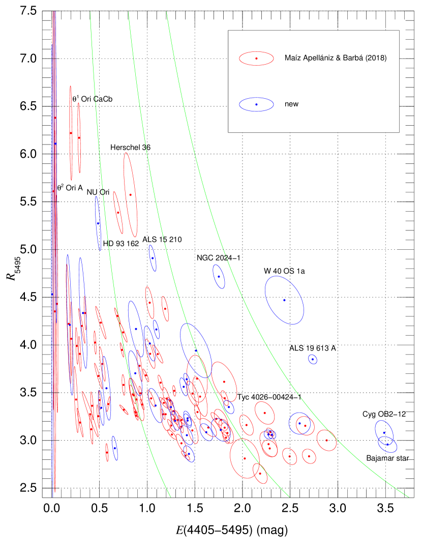
Figure 5: $R_{5495}$ as a function of $E(4405-5495)$ for the sample of 120 OBA stars in this paper. The colour coding indicates whether the data are from paper 0 or new. Some targets discussed in the text are labelled. Green lines correspond (from left to right) to the values of $A_{5495}$ of 3, 6, and 9 mag.

 Before we analyse our results for the 7700 Å absorption band, we start with a discussion on the general optical-NIR extinction of our sample, which is relevant to what will be studied later. In subsection 3.3 of paper 0 we analysed the distribution of extinguished OB stars in the $E(4405-5495)$-$R_{5495}$ plane. Here we follow up on those results with the new values calculated for OBA stars, which are given in Table. 3, along with those for the sample in common between the two papers. Fig. 5 is the equivalent to Fig. 9 in paper 0 but with a different choice of representation. Rather than plotting the error bars for $E(4405-5495)$ and $R_{5495}$ for each star we plot now the uncertainty ellipse, including the correlation between the two quantities as derived by CHORIZOS. As noted in Appendix C of paper 0, the values of $E(4405-5495)$ and $R_{5495}$ derived from optical+IR photometry are usually anticorrelated and that is clearly seen in Fig. 5. As the ellipses are elongated in a direction close to the one defined locally by the line of constant $A_{5495}$, the result is that the relative uncertainty in $A_{5495}$ is usually less than that of $E(4405-5495)$ or $R_{5495}$. In other words, the CHORIZOS calculation constraints $A_{5495}$ better than either $E(4405-5495)$ or $R_{5495}$.

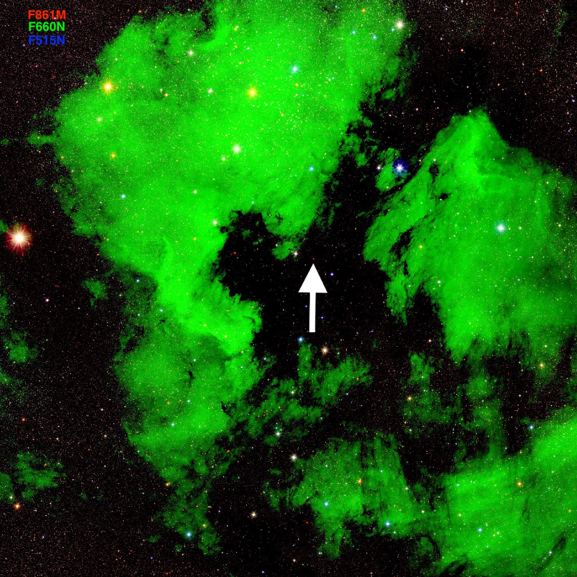
Figure 6: The North America and Pelican nebulae as imaged by the GALANTE survey (Maíz Apellániz et al., 2019a; Lorenzo-Gutiérrez et al., 2019). The Bajamar star, responsible for most of the ionizing photons, is the red object indicated by the arrow, hidden behind the molecular cloud that creates the Atlantic Ocean and Gulf of Mexico and that also obscures the unseen nebulosity and background stars. Most of the stars in the bright part of the nebulae have little extinction. The three-filter combination is composed of a Calcium triplet band (red), H$\alpha$ (green), and narrow-$V$ (blue). The field size is 3.2${}^{\rm o}\times$3.2^o (40 pc $\times$ 40 pc for a distance of 714 pc, Maíz Apellániz et al. submitted to A&A) and is composed of several GALANTE fields, whose detector has a size of 1.4${}^{\rm o}\times$1.4^o. North is up and East is left.

   

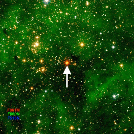
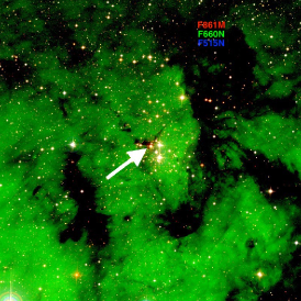
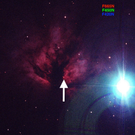
Figure 7: Three objects in our sample imaged by the GALANTE survey (Maíz Apellániz et al., 2019a; Lorenzo-Gutiérrez et al., 2019). [left] Cyg OB2-12 in Cyg OB2, where other stars in our sample are also located. Cyg OB2-12 has some additional extinction with respect to the rest of the association, visible in the image as a dimming of the pervasive but diffuse nebular emission and by the distinct redder colour of the star. [center] Tyc 4026-00424-1 in Berkeley 59, which also contains other stars in our sample. Tyc 4026-00424-1 sits behind a dust lane and is redder than the surrounding OB stars. [right] NGC 2024-1 in the Flame nebula is in the bright part of the H ii region but adjacent to the dust lane that completely blocks its optical emission towards the East. The extremely bright source is $\zeta$ Ori, which contains two O stars and one of B type (Hummel et al., 2013; Maíz Apellániz et al., 2018a) and is actually at a similar distance as the Flame nebula (Zari et al., 2019), which demonstrates the effect of differential extinction. The three fields are 29′$\times$29′, which corresponds to linear sizes of 14.5 pc, 9.4 pc, and 3.4 pc, respectively. North is up and East is left. The first two panels use the same filter combination as Fig. 6 while the third one is a combination of H$\alpha$ continuum (red), continuum between H$\gamma$ and H$\beta$ (green) and continuum between H$\delta$ and H$\gamma$ (blue). The nebulosity seen originating in NGC 2024 corresponds to a mixture of nebular continuum and some weak lines such as He i $\lambda$6680. Arrows indicate the object in each panel.

There are two main novelties in Fig. 5 with respect to paper 0. The first one is the presence of two stars at higher $E(4405-5495)$ (Bajamar star, Fig. 6, and Cyg OB2-12, Fig. 7) than any of the ones there. Both objects follow the trend discussed in paper 0 and also followed by the majority of the stars here, for which the average $R_{5495}$ per $E(4405-5495)$ bin decreases as $E(4405-5495)$ increases, with the highest bins having averages close to $R_{5495}$ = 3.0. On the other hand, there are three new stars that break that trend (NGC 2024-1, Fig. 7; W 40 OS 1a; and ALS 19 613 A) and appear in the previously empty region with $\mbox{$E(4405-5495)$}>1.7$ mag and $\mbox{$R_{5495}$}>3.8$ i.e. they are objects with simultaneously large values of $E(4405-5495)$ and $R_{5495}$. What do these three objects have in common? They are all in the nebular-bright part of H ii regions (NGC 2024, W 40, and M17, respectively) but with a line of sight that passes close to the molecular cloud. Indeed, other objects located towards the left and upwards from them in the plot (ALS 15 210, HD 93 162, and Herschel 36, the first two in the Carina nebula and the third in M8) share the same characteristic. Continuing in that direction in Fig. 5 towards lower values of $E(4405-5495)$ we find three of the stars in the Orion nebula ($\theta^{1}$ Ori Ca,Cb and $\theta^{2}$ Ori A) and the nearby M43 (NU Ori). These nine stars that depart from the general $E(4405-5495)$-$R_{5495}$ trend will be referred in the next subsection as the high-$R_{5495}$ subsample. This reinforces our conclusion from paper 0: regions with high levels of UV radiation have large values of $R_{5495}$. The novelty here is that we have apparently found the condition required for large amounts of high-$R_{5495}$ dust to exist: there must be a nearby molecular cloud to act as a source. As we proposed in Maíz Apellániz 2015 and in paper 0, the grains that were originally in the protected molecular environment are exposed to the intense UV radiation from the nearby O star(s) and the small grains (mostly PAHs, Tielens 2008) are selectively destroyed, leaving behind the large grains responsible for the high values of $R_{5495}$.

Objects with very high values of $A_{5495}$ in Table 3 have large values of $\chi^{2}_{\rm red}$. This is likely a sign that for $A_{5495}$$\sim$10 mag the Maíz Apellániz et al. (2014) family of extinction laws is starting to lose its accuracy, something that was expected, and that signals the need for an improved family of optical extinction laws, an issue that we will tackle in future papers of this series. For our immediate needs, we can consider that the uncertainties in the extinction parameters in Table 3 are likely underestimated by a factor of 2–3 for the four stars with $A_{5495}$$\sim$10 mag.

4.2 The 7700 Å absorption band

 We start our analysis of the 7700 Å absorption band by plotting its EW as a function of $A_{5495}$ (Fig. 8) and of EW${}_{{\rm K\,I\,}\lambda 7701.093}$ (Fig. 9), two different measurements of the amount of intervening material in the ISM along the line of sight. In both cases there is a significant correlation but it is readily apparent that it is stronger for $A_{5495}$ than for EW${}_{{\rm K\,I\,}\lambda 7701.093}$. In some stars the different saturation levels of the line for different ISM kinematics may be at play for EW${}_{{\rm K\,I\,}\lambda 7701.093}$ (see Appendix A) but this effect cannot be the whole story, as even for relatively narrow lines (W${}_{90}<$ 0.6 Å) the Pearson correlation coefficient is just 0.601. On the other hand, the Pearson correlation coefficient between $A_{5495}$ and EW₇₇₀₀ is 0.633 for the sample of 120 OBA stars and if we exclude the 12 named stars in Fig. 8 it goes up to 0.814. The twelve excluded stars are the nine that depart from the general trend in Fig. 5, the two objects with the highest $E(4405-5495)$ there (see previous subsection), and Tyc 4026-00424-1 (below we describe their special circumstances). This is a first sign that the 7700 Å absorption band is possibly related to the dust that extinguishes the stellar continuum but the existence of some outliers indicates that there must be at least one difference between its carrier and dust particles in general.

Something else we can notice in Fig. 8 is that the two red giants appear to follow the same general trend as the OBA stars, a sign that the carrier appears to be in the general ISM and not in clouds specifically associated with OBA stars. Of course, two objects are a small sample that needs to be increased to confirm whether that hypothesis is correct (we have GO 15 816 observations pending so we should confirm this in the near future). Another, perhaps more important, effect can also be seen in Fig. 8, where we have colour-coded objects by their membership to a given region. With a few exceptions, what we see is that for a given region there is little variation in EW₇₇₀₀ despite large changes in $A_{5495}$, i.e. the correlation between $A_{5495}$ and EW₇₇₀₀ disappears when only objects in the same region are considered. For example, targets in Cyg OB2 (Fig. 7) have values of $A_{5495}$ between $\sim$4 mag and $\sim$11 mag but EW₇₇₀₀ is close to 15 Å for most objects and the two at the extremes of the EW₇₇₀₀ distribution have intermediate values of $A_{5495}$. Even more extremely, stars in Orion span an extinction range from close to zero to more than 8 mag in $A_{5495}$ while keeping EW₇₇₀₀ around 1–2 Å with the single exception of the intermediate extinction NU Ori, the only one with a slightly higher value. This prompts our hypothesis with respect to the carrier of the 7700 Å band: it is strongly depleted in the ISM associated with young star-forming regions such as the ones where OB stars are usually located.

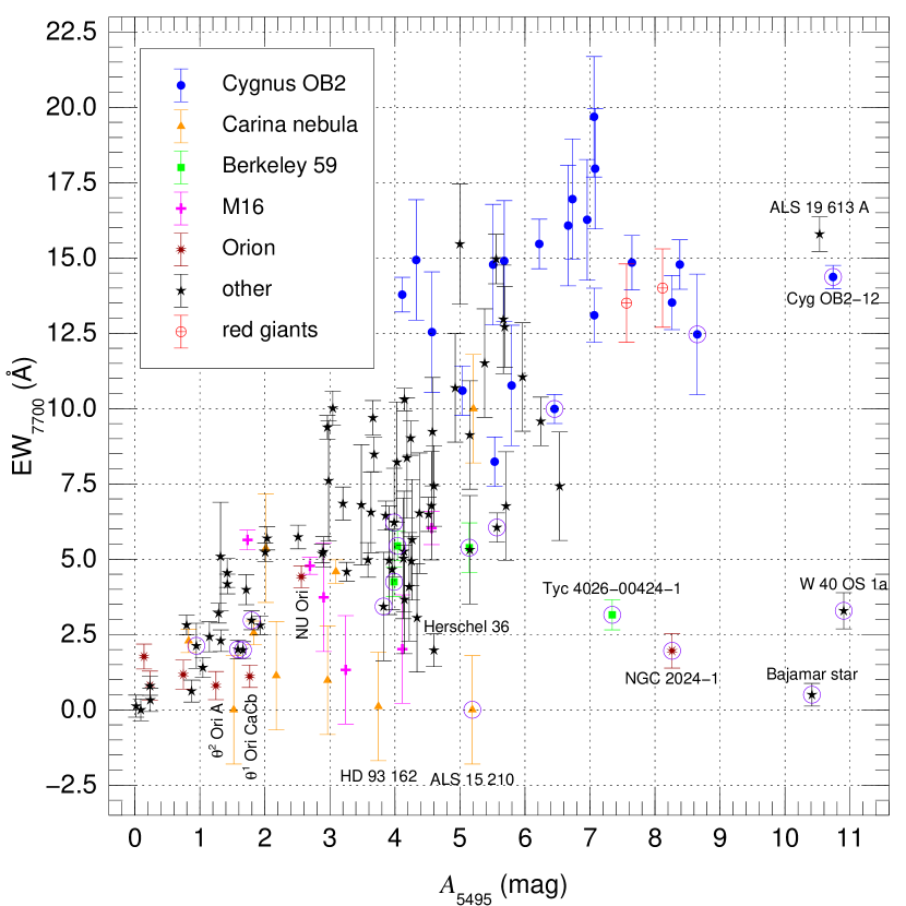
Figure 8: EW₇₇₀₀ as a function of $A_{5495}$ for the full sample in this paper. The colour coding indicates specific regions in the sky and the two red giants. In addition, objects with a purple circle around them have C₂ in absorption detected in Table 6. Orion refers to the whole region (e.g. Zari et al. 2019), not to the Orion nebula alone. Some targets discussed in the text are labelled.

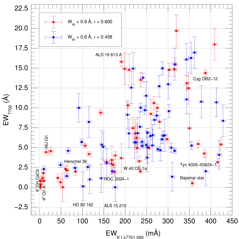
Figure 9: EW₇₇₀₀ as a function of EW${}_{{\rm K\,I\,}\lambda 7701.093}$ for the sample of 120 OBA stars in this paper. Symbols are colour-coded by W₉₀ for K i $\lambda$7701.093. Pearson correlation coefficients for the two subsets are given in the legend. Some targets discussed in the text are labelled.

In order to verify that hypothesis we now turn to another one of our measured quantities, that of the (3,0) C₂ Phillips band lines. As shown in the Appendix (Table 6), we have only detected them in 18 of our 120 OBA stars (15% of the sample), indicating that most sightlines do not have significant amounts of molecular carbon and that most of the dust is associated with low/intermediate density regions in the ISM. However, those 18 detections include the four objects that depart more clearly from the general trend in Fig. 8, i.e. those with $A_{5495}$ $>$ 6 mag and EW₇₇₀₀ $<$ 5 Å: Tyc 4026-00424-1, NGC 2024-1, Bajamar star, W 40 OS 1a. Furthermore, W 40 OS 1a is the target with the highest measured C₂ line intensity in our sample and with one of the two highest departures from the general trend in Fig. 8 and all four of them are among the highest EWs in Table 6. In general, the 18 detections, shown with purple circles in Fig. 8, are located towards the right with respect to the general trend in that plot. Therefore, there is a clear correlation between the departure of EW₇₇₀₀ from its expected value for a given amount of extinction and the EW for the $Q$(2) (3,0) C₂ Phillips band line. This allows us to refine the hypothesis about the carrier of the 7700 Å band: it is strongly depleted in the molecular clouds rich in C₂ in young star-forming regions.

Let us analyse the circumstances of the four stars mentioned in the previous paragraph. They all share two characteristics: (a) they are relatively close to the Sun compared to the sample average (Tyc 4026-00424-1 is the most distant one, at $\sim$1.1 kpc, most targets in our sample such as those in Cyg OB2, the Carina nebula, or M16 are beyond that) and (b) when nearby stars have been measured they show considerably lower extinctions, e.g. most stars in the Orion region or in the bright parts of the North America nebula have low values of $E(4405-5495)$. That combination implies that they are affected mostly by local extinction but that most of the sightline towards each star is relatively dust-free. Indeed, that is what the GALANTE images in Figs. 6 and 7 show (see Herczeg et al. 2019 for the similar W 40 circumstances): the four stars are either behind dust lanes (where C₂ is likely to reside) or close to them, which likely means that due to projection effects the sightline crosses both the bright nebulosity and the molecular gas. This reinforces our hypothesis regarding the carrier of the 7700 Å band.

What about the other stars with strong C₂ absorptions? Two of them are Cyg OB2-12 and Cyg OB2-B17. They are the most extinguished stars from Cyg OB2 in our sample but their values of EW₇₇₀₀ are average for the association. The most likely explanation is that there is a large extinction dispersed along the sightline (which coincides with the Cygnus arm) that affects all of the association but that those two stars have nearby molecular gas (see Fig. 7 for Cyg OB2-12) that introduces the extra extinction and the C₂ lines without contributing significantly to EW₇₇₀₀. Also, all four stars in Berkeley 59 (the previously mentioned Tyc 4026-00424-1 but also BD $+$66 1674, BD $+$66 1675, and V747 Cep) have intense C₂ absorption. We already pointed out in paper 0 that this cluster had a very high extinction for its distance and that it was likely that “most of the extinction common to the four sightlines is coming from a molecular cloud that affects all sightlines”, a prediction that we confirm here with this detection. An additional star with a strong C₂ absorption is LS III $+$46 11 in Berkeley 90, which was analysed in detail in Maíz Apellániz et al. (2015). They proposed there (Fig. 4 in that paper) that the star experiences a local additional extinction that does not affect the nearby LS III $+$46 12 (where we do not detect C₂ absorption) and that is caused by the core of a cloud that is typical of a $\zeta$-type DIB sightline. Such clouds are shielded from UV radiation, as opposed to those of $\sigma$-type sightlines, which are exposed to UV radiation (Krełowski et al., 1997; Cami et al., 1997). This also reinforces our hypothesis, as the values of EW₇₇₀₀ for those two stars in Berkeley 90 are just $\sim$1 sigma apart from each other, indicating that the local additional extinction that affects LS III $+$46 11 produces little effect in the 7700 Å band.

The Berkeley 90 study by Maíz Apellániz et al. (2015) prompts us to look into the relationship between the 7700 Å band and DIBs. As we previously mentioned, the band is much wider that any known DIB but it is worth noting that close to its central wavelength Jenniskens & Desert (1994) describe a DIB with central wavelength of 7711.8 Å (vacuum) and a FWHM of 33.5 Å (five and a half times narrower than our measurement). It is likely that this DIB was the central part of the 7700 Å band with the rest flattened by the spectrum rectification. The more recent compilations of Sonnentrucker et al. (2018) and Fan et al. (2019) do not include any broad DIBs in the vicinity. At a more general level, the characteristics we have described in the previous paragraphs indicate that the behaviour of the 7700 Å band is similar to that of $\sigma$-type DIBs. That is, it originates in a carrier present in the low/intermediate density regions of the ISM exposed to UV radiation but is depleted in the dense, shielded regions. We leave for a future study an analysis of this relationship between $\zeta$+$\sigma$ DIBs and the 7700 Å band with a large sample. Here we simply point to the behaviour of EW₇₇₀₀ in the two prototype sightlines (from whose Bayer Greek letter receive their names): $\sigma$ Sco Aa,Ab (a complex multiple system dominated by a B1 III star, Morgan et al. 1953; Grellmann et al. 2015) and $\zeta$ Oph (a runaway late-O star, Hoogerwerf et al. 2001; Maíz Apellániz et al. 2018b). Both have similar values of $E(4405-5495)$ but $\sigma$ Sco Aa,Ab has an EW₇₇₀₀ approximately double that of $\zeta$ Oph. Therefore, the current data indicate a similar behaviour for the 7700 Å band and $\sigma$-type DIBs and, hence, a possible common carrier. Another line of study that we plan to pursue in the future is the relationship between the 7700 Å band and the so-called C₂-DIBs (Thorburn et al., 2003; Elyajouri et al., 2018), which appear to be associated with high column densities of molecular carbon.

4.3 An ISM model

 Here we analyse the relationship between the 7700 Å band and $R_{5495}$. We recall that in the previous section we identified nine stars that depart from the general $E(4405-5495)$-$R_{5495}$ trend (the high-$R_{5495}$ subsample). Eight of those stars follow a nearly-horizontal trend in Fig. 8 and include two of the four extreme objects in the lower right corner of that figure. This suggests a connection between the 7700 Å band and dust grain size, with the carrier being depleted in regions of high $R_{5495}$. The relationship is not perfect, though, as two stars in the lower right corner of the figure (Tyc 4026-00424-1 and Bajamar star) have normal values of $R_{5495}$ and ALS 19 613 A has simultaneously high $R_{5495}$ and normal EW₇₇₀₀ values. A hypothesis that fits the data describes the five objects in our sample with high extinction in H ii regions by dividing them in three groups: [a] stars where the sightline places them behind the parent molecular cloud (Tyc 4026-00424-1 and Bajamar star), [b] stars with a mixed sightline or in a transition region with high $R_{5495}$ and low EW₇₇₀₀ (NGC 2024-1 and W 40 OS 1a), and [c] stars with high $R_{5495}$ and normal EW₇₇₀₀ (ALS 19 613 A). Objects in the first group experience “molecular-cloud extinction” with low $R_{5495}$, little or no carrier of the 7700 Å band, and C₂ absorption. For those in the second group destruction of small grains has started (increasing $R_{5495}$) but C₂ is still present and the production of the carrier of the 7700 Å band has not started. Finally, in the third group the carrier of the 7700 Å band already exists and C₂ is likely destroyed, producing an “H ii-region extinction” with high $R_{5495}$, presence of the 7700 Å-band carrier, and no molecular carbon. Away from H ii regions we have the general trend in $E(4405-5495)$-$R_{5495}$ that goes from $R_{5495}$ of 4.0-4.5 for low $E(4405-5495)$ (with a high dispersion) to values of 3.0 for high $E(4405-5495)$. In paper 0 we proposed that this trend is an effect of the increasing density and decreasing UV radiation field as one goes from the diffuse to the translucent ISM (e.g. Fig. 1 in Snow & McCall 2006) that dominates extinction for most Galactic sightlines. That “typical” extinction has no C₂ and the 7700 Å band is present throughout, either in the high-$R_{5495}$ environment of the Local Bubble and similar diffuse ISM regions or in the denser clouds that produce an $R_{5495}$ close to 3.0.

The model described in the previous paragraph should be tested with better data, especially with high-extinction stars in H ii regions. For the stars in H ii regions in the high-$R_{5495}$ subsample not mentioned there we can assign such a classification (molecular-cloud, intermediate, or H ii-region extinctions) based on their location in Fig. 8, with HD 93 162, Herschel 36, and ALS 15 210 (for which we indeed detect C₂ in absorption) in the second group; NU Ori in the third; and $\theta^{1}$ Ori Ca,Cb and $\theta^{2}$ Ori A in either the second or third. Spectra with higher S/N (the values in our current data change significantly from star to star) are required to better detect C₂ and observations of more stars are needed to test the model. However, we expect the real world to be more complicated. In a real sightline, extinction is produced not in a single phase of the ISM but in a combination of them. While absorption structures (whether atomic, molecular, DIB, or the new band) can be superimposed on a spectrum being present in just one of the phases (and diluted in the rest if the carrier is not present there), the value of $R_{5495}$ is a weighted average of the individual values of each phase of the ISM (see Appendix C of Maíz Apellániz et al. (2014), note this is true for families of extinction laws of the form $A_{\lambda}/\mbox{$A_{5495}$}=a(\lambda)+b(\lambda)/\mbox{$R_{5495}$}$). Therefore, as information from different phases is preserved (although diluted) in the absorption structures but simply combined into $R_{5495}$ to give an average, it should be possible to combine ISM phases to build two sightlines with identical $R_{5495}$ but different absorption spectra. $R_{5495}$ can be correlated with values derived from ISM absorption lines but the correlation can never be perfect (Fig. 5 in Maíz Apellániz 2015). The identity of the carrier of the 7700 Å band is unknown at this time but we know it is abundant in typical ISM sightlines and depleted in those with abundant molecular gas and that is possibly the same as that of the $\sigma$-type DIBs.

5 Summary and future work

 In this work we report the discovery of a broad interstellar band centred around 7700 Å that had remained hidden behind an O₂ telluric band. Its equivalent width correlates well with the amount of extinction but deviates from the correlation for some sightlines, particularly those that are rich in molecular carbon, where its values are lower. A similar depletion of its carrier in such dense environments also takes place for $\sigma$-type DIBs, pointing towards a possible common origin for both types of ISM absorption features. We also extend the model of paper 0 to describe the different types of extinction that take place in star-forming regions with two extreme types: a “molecular-cloud extinction” with low $R_{5495}$, low EW₇₇₀₀, and C₂ absorption and an “H ii-region extinction” with high $R_{5495}$, high EW₇₇₀₀, and no C₂ absorption, with some sightlines falling between the two extremes. Away from star-forming regions, the 7700 Å band is ubiquitous, C₂ is absent, and $R_{5495}$ decreases as the density of the medium increases and the UV radiation field decreases. Our results are based on 26, 30, and 120 stars observed with low-resolution long-slit space-based STIS, intermediate-resolution IFU ground-based FRODOspec, and high-resolution échelle ground-based spectroscopy, respectively. In future papers we plan to address the detailed behaviour of the extinction law in the optical range using spectrophotometry, connect the optical and IR extinction laws, and analyse a large sample of interstellar absorption lines to produce a better understanding of the relationship between extinction and the different phases of the ISM.

Data availability

 This paper uses observations made with the ESA/NASA Hubble Space Telescope, obtained from the data archive at the Space Telescope Science Institute. STScI is operated by the Association of Universities for Research in Astronomy, Inc. under NASA contract NAS 5-26 555. The ground-based spectra in this paper have been obtained with the 2.2 m Observatorio de La Silla Telescope, the 3.5 m Telescope at the Observatorio de Calar Alto (CAHA), and three telescopes at the Observatorio del Roque de los Muchachos (ORM): the 1.2 m Mercator Telescope (MT), the 2.0 m Liverpool Telescope (LT), and the 2.5 m Nordic Optical Telescope (NOT). Some of the MT and NOT data were obtained from the IACOB spectroscopic database (Simón-Díaz et al., 2011a; Simón-Díaz et al., 2011b, 2015). The GALANTE images were obtained with the JAST/T80 telescope at the Observatorio Astrofísico de Javalambre, Teruel, Spain (owned, managed, and operated by the Centro de Estudios de Física del Cosmos de Aragón). No reflective surface with a size of 4 m or larger was required to write this paper. The derived data generated in this research will be shared on reasonable request to the corresponding author for those cases where no proprietary rights exist.

Appendix A ISM lines in the 7400–8000 Å range

Table 4: Main ISM absorption lines in the 7400–8000 Å region (vacuum wavelengths). The last column indicates whether it is a new line (yes), an old one (no), or an old one with new measurements (meas). BIB stands for Broad Interstellar Band.

type $\lambda_{\rm c}$ FWHM new? ($\AA$) ($\AA$) DIB 7434. 1(0.2) 19. 6(0.2) meas K i 7667. 021 — no BIB 7700. 0(1.3) 179. 9(3.8) yes K i 7701. 093 — no DIB 7708. 88(0.03) 0. 71(0.04) meas DIB 7710. 20(0.03) 0. 65(0.03) meas C₂ $R$(6) 7716. 698 — no C₂ $R$(4) 7717. 067 — no C₂ $R$(8) 7717. 539 — no C₂ $R$(2) 7718. 652 — no C₂ $R$(10) 7719. 594 — no C₂ $R$(0) 7721. 454 — no DIB 7722. 58(0.07) 3. 70(0.09) meas DIB 7724. 03(0.01) 0. 79(0.01) meas C₂ $Q$(2) 7724. 221 — no C₂ $Q$(4) 7726. 345 — no C₂ $P$(2) 7727. 945 — no C₂ $Q$(6) 7729. 684 — no C₂ $P$(4) 7733. 791 — no C₂ $Q$(8) 7734. 245 — no C₂ $Q$(10) 7740. 033 — no C₂ $P$(6) 7740. 867 — no C₂ $P$(8) 7749. 169 — no DIB 7929. 9(0.1) 9. 8(0.3) meas

Table 5: Results for the ISM absorption line K i $\lambda$7701.093.

star code EW $v$ W₉₀ $\frac{{\rm EW}_{7701.093}}{{\rm EW}_{7667.021}}$ (mÅ) (km/s) (Å) $\delta$ Ori Aa,Ab H 1$\pm$ 1 — — — $\mu$ Col NH 1$\pm$ 1 — — — $\lambda$ Lep H 2$\pm$ 2 — — — 15 Mon Aa,Ab H 2$\pm$ 2 — — — $\rho$ Leo A,B H 3$\pm$ 3 — — — $\theta^{1}$ Ori Ca,Cb FNH 7$\pm$ 3 $+$19.5$\pm$ 0.3 0.30 0.620$\pm$ 0.398 $\sigma$ Ori Aa,Ab,B CF 9$\pm$ 4 $+$21.9$\pm$ 0.3 0.34 0.398$\pm$ 0.205 HD 93 028 F 10$\pm$ 5 $+$4.2$\pm$ 0.4 0.62 0.270$\pm$ 0.200 $\theta^{2}$ Ori A FH 10$\pm$ 4 $+$19.4$\pm$ 0.3 0.38 0.484$\pm$ 0.289 NU Ori H 15$\pm$ 5 $+$23.9$\pm$ 0.4 0.28 0.392$\pm$ 0.234 $\sigma$ Sco Aa,Ab F 26$\pm$ 5 $-$6.6$\pm$ 0.4 0.37 0.631$\pm$ 0.314 $\lambda$ Ori A CFH 42$\pm$ 3 $+$24.8$\pm$ 0.3 0.28 0.477$\pm$ 0.043 HD 164 402 N 49$\pm$ 5 $-$9.5$\pm$ 0.4 0.70 0.557$\pm$ 0.132 HD 46 966 Aa,Ab H 49$\pm$ 5 $+$18.3$\pm$ 0.4 0.50 0.522$\pm$ 0.117 HD 93 205 F 54$\pm$ 5 $+$4.1$\pm$ 0.4 0.55 0.548$\pm$ 0.117 9 Sgr A,B FH 60$\pm$ 4 $-$6.9$\pm$ 0.3 0.42 0.609$\pm$ 0.064 $\alpha$ Cam C 63$\pm$ 5 $-$4.5$\pm$ 0.4 0.63 0.521$\pm$ 0.090 $\zeta$ Oph FN 64$\pm$ 4 $-$15.0$\pm$ 0.3 0.24 0.723$\pm$ 0.082 CPD $-$59 2591 F 67$\pm$ 5 $+$1.1$\pm$ 0.4 0.71 0.522$\pm$ 0.086 HD 34 656 C 83$\pm$ 5 $+$5.4$\pm$ 0.4 0.64 0.625$\pm$ 0.096 Herschel 36 FN 84$\pm$ 4 $-$5.4$\pm$ 0.3 0.30 0.727$\pm$ 0.063 V662 Car F 92$\pm$ 5 $-$6.3$\pm$ 0.4 0.85 0.478$\pm$ 0.054 CE Cam CH 98$\pm$ 4 $-$9.8$\pm$ 0.3 0.60 0.506$\pm$ 0.028 HD 93 162 F 101$\pm$ 5 $-$9.2$\pm$ 0.4 0.98 0.553$\pm$ 0.063 HD 192 639 NH 106$\pm$ 4 $-$13.2$\pm$ 0.3 0.41 0.676$\pm$ 0.043 HD 93 250 A,B F 113$\pm$ 5 $-$5.8$\pm$ 0.4 0.78 0.537$\pm$ 0.054 BD $-$16 4826 N 115$\pm$ 5 $-$4.7$\pm$ 0.4 0.73 0.519$\pm$ 0.049 HD 46 150 F 115$\pm$ 5 $+$23.6$\pm$ 0.4 0.48 0.592$\pm$ 0.063 CPD $-$59 2626 A,B F 117$\pm$ 5 $-$0.2$\pm$ 0.4 1.01 0.626$\pm$ 0.068 HD 149 452 F 143$\pm$ 5 $-$15.8$\pm$ 0.4 0.51 0.578$\pm$ 0.048 HD 93 129 Aa,Ab F 144$\pm$ 5 $-$7.5$\pm$ 0.4 1.08 0.594$\pm$ 0.050 HD 93 161 A F 145$\pm$ 5 $-$1.8$\pm$ 0.4 0.81 0.632$\pm$ 0.056 HDE 326 329 F 149$\pm$ 5 $-$4.9$\pm$ 0.4 0.90 0.634$\pm$ 0.055 HD 48 279 A F 156$\pm$ 5 $+$24.4$\pm$ 0.4 0.54 0.736$\pm$ 0.069 HDE 322 417 F 157$\pm$ 5 $-$12.9$\pm$ 0.4 0.87 0.602$\pm$ 0.048 AE Aur H 168$\pm$ 5 $+$14.7$\pm$ 0.4 0.37 0.771$\pm$ 0.070 CPD $-$47 2963 A,B F 169$\pm$ 5 $+$19.8$\pm$ 0.4 0.29 0.771$\pm$ 0.070 $\lambda$ Cep NH 170$\pm$ 4 $-$15.1$\pm$ 0.3 0.87 0.649$\pm$ 0.025 HD 199 216 H 172$\pm$ 5 $-$12.3$\pm$ 0.4 0.29 0.795$\pm$ 0.073 NGC 2024-1 N 175$\pm$ 5 $+$27.6$\pm$ 0.4 0.43 0.730$\pm$ 0.061 ALS 15 210 F 177$\pm$ 5 $-$12.5$\pm$ 0.4 0.79 0.658$\pm$ 0.050 HD 46 223 H 177$\pm$ 5 $+$25.1$\pm$ 0.4 0.37 0.711$\pm$ 0.057 HDE 319 702 F 191$\pm$ 5 $-$5.4$\pm$ 0.4 0.48 0.665$\pm$ 0.047 ALS 19 613 A C 191$\pm$ 5 $-$3.9$\pm$ 0.4 0.57 0.621$\pm$ 0.041 Cyg OB2-11 N 199$\pm$ 5 $-$10.4$\pm$ 0.4 0.58 0.588$\pm$ 0.036 HDE 319 703 A F 205$\pm$ 5 $-$4.8$\pm$ 0.4 0.72 0.654$\pm$ 0.042 HT Sge FH 206$\pm$ 4 $-$3.8$\pm$ 0.3 0.57 0.715$\pm$ 0.025 ALS 2063 F 209$\pm$ 5 $+$12.3$\pm$ 0.4 1.13 0.564$\pm$ 0.032 Cyg OB2-1 A N 209$\pm$ 5 $-$6.9$\pm$ 0.4 0.53 0.687$\pm$ 0.045 Cyg OB2-15 N 214$\pm$ 5 $-$10.3$\pm$ 0.4 0.60 0.672$\pm$ 0.043 ALS 4962 F 218$\pm$ 5 $-$2.1$\pm$ 0.4 0.41 0.756$\pm$ 0.052 Cyg OB2-20 N 219$\pm$ 5 $-$7.3$\pm$ 0.4 0.61 0.685$\pm$ 0.043 BD $+$36 4063 N 222$\pm$ 5 $-$14.0$\pm$ 0.4 0.64 0.706$\pm$ 0.045 ALS 19 693 F 223$\pm$ 5 $-$5.9$\pm$ 0.4 0.49 0.746$\pm$ 0.050 BD $-$13 4930 F 225$\pm$ 5 $-$8.5$\pm$ 0.4 0.66 0.638$\pm$ 0.037 HD 156 738 A,B F 226$\pm$ 5 $-$5.7$\pm$ 0.4 0.50 0.661$\pm$ 0.039 CPD $-$49 2322 F 228$\pm$ 5 $+$18.1$\pm$ 0.4 0.32 0.778$\pm$ 0.053 BD $-$14 5014 N 229$\pm$ 5 $-$5.2$\pm$ 0.4 1.04 0.639$\pm$ 0.036 W 40 OS 1a C 233$\pm$ 5 $-$9.6$\pm$ 0.4 0.32 0.777$\pm$ 0.051 NGC 1624-2 N 234$\pm$ 5 $-$9.4$\pm$ 0.4 1.11 0.648$\pm$ 0.036 Codes: C, CARMENES; F, FEROS; N, FIES; H, HERMES.

Table 5: (continued).

   star code EW $v$ W₉₀ $\frac{{\rm EW}_{7701.093}}{{\rm EW}_{7667.021}}$ (mÅ) (km/s) (Å) HD 207 198 CH 236$\pm$ 4 $-$14.0$\pm$ 0.3 0.37 0.762$\pm$ 0.025 BD $-$12 4979 CF 236$\pm$ 4 $-$1.9$\pm$ 0.3 0.75 0.638$\pm$ 0.018 Cyg OB2-B18 H 236$\pm$ 5 $-$12.3$\pm$ 0.4 0.45 0.771$\pm$ 0.050 BD $+$60 513 N 239$\pm$ 5 $-$13.7$\pm$ 0.4 0.81 0.580$\pm$ 0.029 HD 217 086 NH 240$\pm$ 4 $-$19.5$\pm$ 0.3 0.67 0.617$\pm$ 0.016 Cyg OB2-4 B N 242$\pm$ 5 $-$8.6$\pm$ 0.4 0.64 0.669$\pm$ 0.037 BD $-$14 4922 N 246$\pm$ 5 $+$2.4$\pm$ 0.4 0.92 0.589$\pm$ 0.029 HDE 319 703 Ba,Bb F 249$\pm$ 5 $-$3.6$\pm$ 0.4 0.67 0.637$\pm$ 0.033 Tyc 8978-04440-1 F 249$\pm$ 5 $-$22.0$\pm$ 0.4 0.95 0.657$\pm$ 0.035 HD 168 076 A,B F 252$\pm$ 5 $-$5.7$\pm$ 0.4 0.72 0.663$\pm$ 0.035 HD 168 112 A,B FN 252$\pm$ 4 $-$0.1$\pm$ 0.3 0.83 0.664$\pm$ 0.018 LS I $+$61 303 N 252$\pm$ 5 $-$13.4$\pm$ 0.4 1.28 0.688$\pm$ 0.038 LS III $+$46 12 NH 256$\pm$ 4 $-$16.0$\pm$ 0.3 0.60 0.721$\pm$ 0.020 HD 194 649 A,B NH 259$\pm$ 4 $-$17.4$\pm$ 0.3 0.98 0.648$\pm$ 0.016 HDE 323 110 F 260$\pm$ 5 $-$8.4$\pm$ 0.4 0.56 0.660$\pm$ 0.034 BD $-$14 5040 N 263$\pm$ 5 $+$0.6$\pm$ 0.4 0.70 0.777$\pm$ 0.046 MY Ser Aa,Ab F 264$\pm$ 5 $-$1.1$\pm$ 0.4 0.73 0.701$\pm$ 0.037 Cyg OB2-8 A NH 267$\pm$ 4 $-$9.2$\pm$ 0.3 0.55 0.694$\pm$ 0.018 BD $+$61 487 N 268$\pm$ 5 $-$19.4$\pm$ 0.4 1.43 0.619$\pm$ 0.029 BD $-$11 4586 CF 274$\pm$ 4 $-$4.5$\pm$ 0.3 0.75 0.655$\pm$ 0.016 Cyg OB2-5 A,B NH 275$\pm$ 4 $-$9.6$\pm$ 0.3 0.45 0.758$\pm$ 0.021 HD 168 075 FN 276$\pm$ 4 $-$5.2$\pm$ 0.3 0.74 0.686$\pm$ 0.017 Tyc 7370-00460-1 FN 279$\pm$ 4 $-$6.3$\pm$ 0.3 0.78 0.723$\pm$ 0.019 Cyg OB2-7 NH 280$\pm$ 4 $-$9.9$\pm$ 0.3 0.56 0.712$\pm$ 0.018 V479 Sct FN 282$\pm$ 4 $+$2.4$\pm$ 0.3 0.61 0.722$\pm$ 0.018 BD $-$13 4923 FN 286$\pm$ 4 $-$3.1$\pm$ 0.3 0.85 0.629$\pm$ 0.014 Sh 2-158 1 NH 287$\pm$ 4 $-$26.9$\pm$ 0.3 1.41 0.557$\pm$ 0.011 HD 166 734 F 289$\pm$ 5 $-$6.8$\pm$ 0.4 0.67 0.742$\pm$ 0.038 BD $+$62 2078 N 292$\pm$ 5 $-$16.0$\pm$ 0.4 0.62 0.729$\pm$ 0.036 LS III $+$46 11 NH 297$\pm$ 4 $-$15.6$\pm$ 0.3 0.55 0.714$\pm$ 0.017 ALS 18 748 F 301$\pm$ 5 $-$22.7$\pm$ 0.4 1.08 0.623$\pm$ 0.026 Pismis 24-1 A,B F 302$\pm$ 5 $-$10.6$\pm$ 0.4 1.46 0.713$\pm$ 0.034 Cyg OB2-A11 NH 303$\pm$ 4 $-$9.3$\pm$ 0.3 0.46 0.796$\pm$ 0.021 Cyg X-1 N 308$\pm$ 5 $-$12.0$\pm$ 0.4 0.75 0.698$\pm$ 0.032 BD $-$13 4929 F 310$\pm$ 5 $-$5.8$\pm$ 0.4 0.65 0.725$\pm$ 0.034 ALS 15 108 A,B H 315$\pm$ 5 $-$10.6$\pm$ 0.4 0.42 0.814$\pm$ 0.042 HD 15 570 CH 316$\pm$ 4 $-$12.8$\pm$ 0.3 1.11 0.686$\pm$ 0.015 ALS 19 307 N 316$\pm$ 5 $-$5.5$\pm$ 0.4 0.88 0.665$\pm$ 0.028 Cyg OB2-3 A,B NH 317$\pm$ 4 $-$6.3$\pm$ 0.3 0.51 0.745$\pm$ 0.017 ALS 15 133 N 319$\pm$ 5 $-$8.4$\pm$ 0.4 0.57 0.715$\pm$ 0.032 Cyg OB2-73 N 343$\pm$ 5 $-$11.7$\pm$ 0.4 0.70 0.804$\pm$ 0.037 NGC 3603 HST-5 F 343$\pm$ 5 $-$9.6$\pm$ 0.4 0.70 0.703$\pm$ 0.029 Cyg OB2-22 A H 344$\pm$ 5 $-$9.9$\pm$ 0.4 0.45 0.765$\pm$ 0.034 Cyg OB2-B17 N 348$\pm$ 5 $-$8.4$\pm$ 0.4 0.57 0.762$\pm$ 0.033 THA 35-II-42 F 350$\pm$ 5 $+$3.0$\pm$ 0.4 0.54 0.774$\pm$ 0.034 ALS 15 131 N 354$\pm$ 5 $-$7.8$\pm$ 0.4 0.66 0.845$\pm$ 0.040 HD 17 603 CH 355$\pm$ 4 $-$22.5$\pm$ 0.3 1.23 0.666$\pm$ 0.013 Bajamar star CNH 357$\pm$ 3 $-$12.5$\pm$ 0.3 0.46 0.818$\pm$ 0.013 Cyg OB2-22 C N 362$\pm$ 5 $-$9.1$\pm$ 0.4 0.65 0.716$\pm$ 0.028 BD $+$66 1674 NH 370$\pm$ 4 $-$16.5$\pm$ 0.3 0.51 0.769$\pm$ 0.016 Cyg OB2-27 A,B N 378$\pm$ 5 $-$9.3$\pm$ 0.4 0.73 0.704$\pm$ 0.026 BD $+$66 1675 NH 385$\pm$ 4 $-$16.6$\pm$ 0.3 0.52 0.777$\pm$ 0.016 Cyg OB2-12 CH 387$\pm$ 4 $-$9.0$\pm$ 0.3 0.50 0.809$\pm$ 0.017 BD $-$13 4927 F 388$\pm$ 5 $-$3.6$\pm$ 0.4 0.61 0.763$\pm$ 0.030 Cyg OB2-9 N 409$\pm$ 5 $-$9.7$\pm$ 0.4 0.58 0.729$\pm$ 0.026 V889 Cen F 413$\pm$ 5 $-$29.3$\pm$ 0.4 1.32 0.680$\pm$ 0.023 Tyc 4026-00424-1 CH 416$\pm$ 4 $-$16.9$\pm$ 0.3 0.50 0.843$\pm$ 0.017 HDE 326 775 F 420$\pm$ 5 $-$21.2$\pm$ 0.4 0.97 0.670$\pm$ 0.022 V747 Cep NH 424$\pm$ 4 $-$17.3$\pm$ 0.3 0.58 0.758$\pm$ 0.013 KM Cas N 429$\pm$ 5 $-$24.0$\pm$ 0.4 1.52 0.699$\pm$ 0.023 Codes: C, CARMENES; F, FEROS; N, FIES; H, HERMES.

 We list in Table 4 the relevant ISM lines that we have found in the 7400–8000 Å range in our spectra. The most significant contaminant for the measurement of the broad absorption band at 7700 Å is the K i $\lambda\lambda$7667.021,7701.093 doublet. We have measured those two lines in the combined LiLiMaRlin spectra for each star and telescope (as mentioned in the text, different epochs of the same star with the same telescope are used when available to alleviate the effect of telluric lines) and the results are given in Table 5. Given the variety of data and the need to accurately eliminate telluric lines, each line has been measured with an interactive program that allows us to set the continuum and integrating regions. No profiles have been fit, as many stars show multiple kinematic components. Instead, the lines have been integrated to derive their equivalent widths (EWs, used for sorting in the table), central velocities ($v$), and width that contains 90% of the flux (W₉₀). The latter value is selected because, given the complexity of the profiles, it captures the width of the line better than smaller percentages and higher ones may be subject to larger systematic effects for low values of the EW. In Table 5 we show the values for K i $\lambda$7701.093 and the equivalent width ratio with K i $\lambda$7667.021 instead of the opposite for two reasons. First, K i $\lambda$7701.093 is the weaker line (in the high S/N, low intensity regime the equivalent width ratio should be 0.33) so it saturates later and choosing it as the reference allows for a larger dynamic range in the EW. Second and most importantly, K i $\lambda$7667.021 is more affected by O₂ telluric lines and is, therefore, more prone to systematic errors. The uncertainties in all quantities have been calculated from the comparison of the measurements of the same star using different telescopes and they encompass both random and systematic effects but the latter are the dominant ones. When in doubt, we have erred on the side of caution e.g. the uncertainties in the EW are likely overestimated for the stars with low values. For the sample in common with Welty & Hobbs (2001) we find a good agreement for the EWs. The value of W₉₀ for measurements with FEROS (code F in the table) and FIES (code N) have been reduced by 0.05 Å and 0.10 Å, respectively, to account for the lower spectral resolution of those spectrographs. The correction values were determined empirically by comparing stars observed with those spectrographs and with the higher resolution CARMENES (code C) or HERMES (code H).

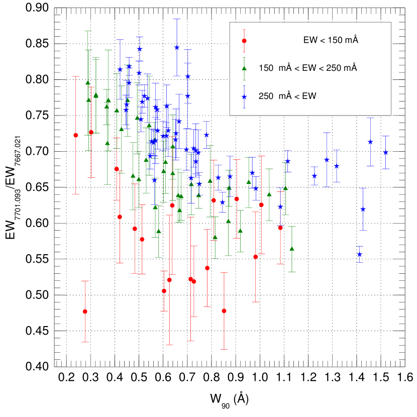
Figure 10: Equivalent-width ratio for the K i doublet as a function of W₉₀ for K i $\lambda$7701.093. Symbols are colour-coded by equivalent width. Objects with uncertainties in the vertical axis greater than 0.1 are not plotted.

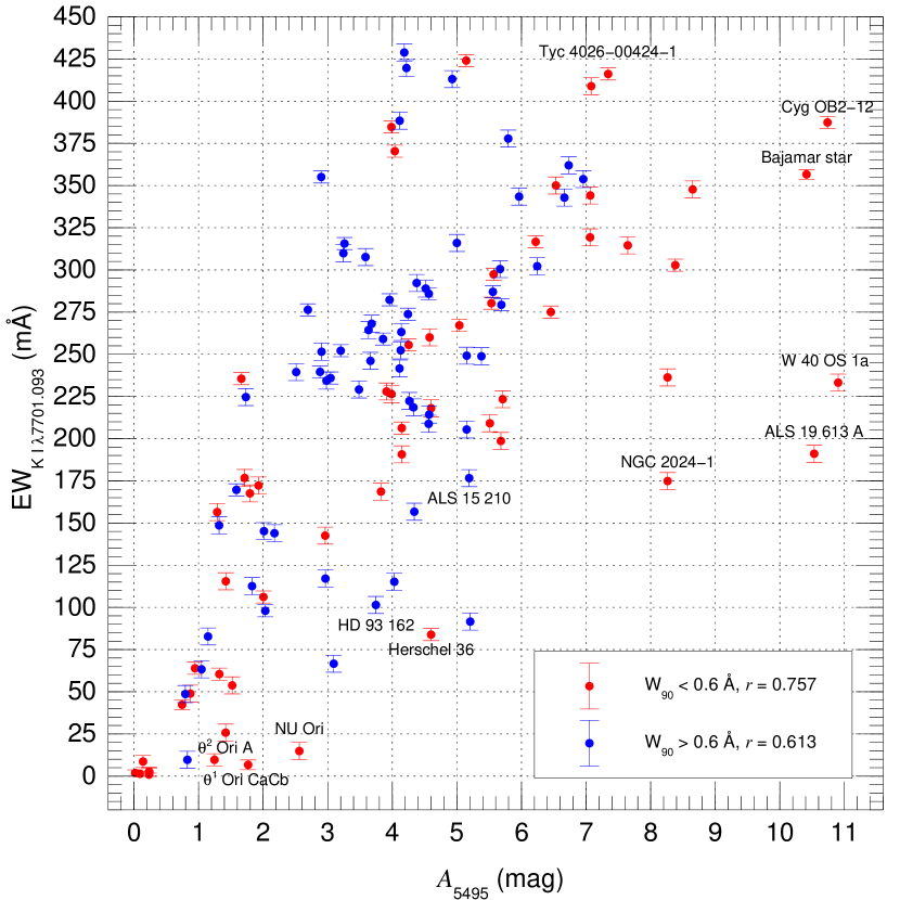
Figure 11: EW${}_{{\rm K\,I\,}\lambda 7701.093}$ as a function of $A_{5495}$. Symbols are colour-coded by W₉₀ for K i $\lambda$7701.093. Pearson correlation coefficients for the two subsets are given in the legend. Some targets discussed in the text are labelled.

Table 5 shows a large range of EW${}_{{\rm K\,I\,}\lambda 7701.093}$, from difficult to detect to more than 0.4 Å. In Fig. 10 we show the relationship between EW${}_{{\rm K\,I\,}\lambda 7701.093}$, W₉₀ for K i $\lambda$7701.093, and the EW ratio. As EW${}_{{\rm K\,I\,}\lambda 7701.093}$ increases, the points move towards the upper right as a result of the increase in saturation of the lines. On the one hand, the flattening at the bottom of the line increases its width and, on the other hand, saturation appears first in K i $\lambda$7667.021 and increases the EW ratio (a curve of growth effect). Within a colour group in Fig. 5, the range of values in W₉₀ corresponds to the different kinematics of the intervening gas: sightlines with single components are located towards the left and those with multiple components towards the right. This has two consequences: the same EW${}_{{\rm K\,I\,}\lambda 7701.093}$ does not correspond to the same amount of intervening material (which is larger for smaller W₉₀ at constant EW${}_{{\rm K\,I\,}\lambda 7701.093}$) and the EW ratio increases for smaller W₉₀, as the two lines are moved towards a flatter part of the curve of growth in the absence of multiple components.

In Fig. 11 we compare EW${}_{{\rm K\,I\,}\lambda 7701.093}$ with the extinction $A_{5495}$ (see main text for its calculation). The two quantities are correlated but there is a significant spread. If we restrict the sample to those objects with “narrow” profiles (W${}_{90}<$ 0.6 Å) the correlation improves, as for wider profiles EW${}_{{\rm K\,I\,}\lambda 7701.093}$ can depend heavily on the particular gas kinematics (many of those sightlines have multiple kinematic components, significantly those in the Carina nebula, see Walborn 1982). However, variations in the column density ratios of dust and K i must also exist, as evident from the existence of some sightlines prominently poor in K i. Several of those cases are in H ii regions so we are likely observing an ionization effect (Welty & Hobbs, 2001), as the ionization potential of potassium is low. In general, EW${}_{{\rm K\,I\,}\lambda 7701.093}$ is not a very good predictor of extinction, especially if the line is narrow. In our sample we have stars with EW${}_{{\rm K\,I\,}\lambda 7701.093}$ of $\approx$ 200 mÅ with $A_{5495}$ from less than 2 mag to more than 10 mag. Conversely, $A_{5495}$ is not a good predictor of the EW${}_{{\rm K\,I\,}\lambda 7701.093}$, especially if the line is wide.

Table 6: EWs for the $Q$(2) (3,0) C₂ Phillips band line at 7724.221 Å.

star code EW notes (mÅ) AE Aur C 1.8$\pm$ 1.2 (2,0) detection by F94 ALS 15 210 F 2.2$\pm$ 1.2 BD $+$66 1674 NH 8.6$\pm$ 0.8 BD $+$66 1675 NH 8.9$\pm$ 0.8 (2,0) detection by v89 Bajamar star CNH 9.4$\pm$ 0.7 CPD $-$47 2963 A,B F 2.2$\pm$ 1.2 Cyg OB2-12 CH 9.0$\pm$ 0.8 detections by v89, G94 Cyg OB2-5 A,B H 4.4$\pm$ 1.2 (1,0) detection by G94 Cyg OB2-B17 N 9.1$\pm$ 1.2 HD 156 738 A,B F 2.3$\pm$ 1.2 not detected by v89 HD 207 198 CH 0.9$\pm$ 0.8 (2,0) detection by v89 LS III $+$46 11 H 6.4$\pm$ 1.2 NGC 2024-1 C 8.5$\pm$ 1.2 Tyc 4026-00424-1 CH 9.3$\pm$ 0.8 V747 Cep NH 9.0$\pm$ 0.8 W 40 OS 1a C 19.6$\pm$ 1.2 $\lambda$ Cep N 0.6$\pm$ 0.6 (2,0) detection by v89 $\zeta$ Oph NH 0.5$\pm$ 0.5 (2,0) detection by v89 Codes: C, CARMENES; F, FEROS; N, FIES; H, HERMES. v89: van Dishoeck & Black (1989). F94: Federman et al. (1994). G94: Gredel & Münch (1994).

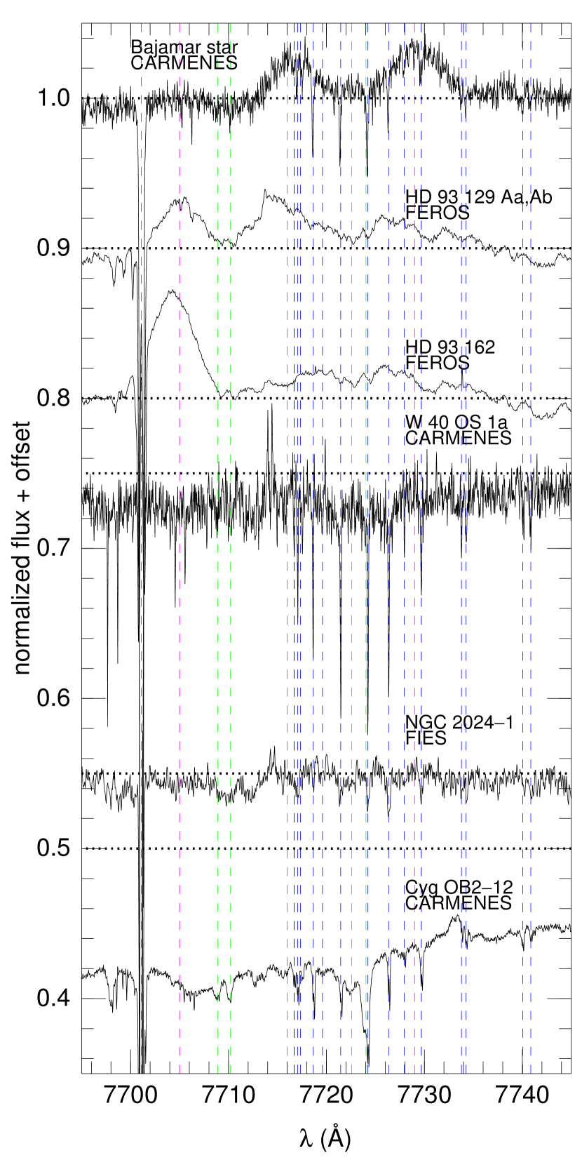
Figure 12: Sample échelle spectra to showcase the rich ISM and stellar spectra in the 7695–7745 Å region. Red, blue, green, and magenta mark the position of atomic, molecular, DIB, and stellar lines, respectively, the first three (ISM) lines in absorption and the last (stellar) in emission. The thick dashed horizontal lines mark the position of the continua (note that Cyg OB2-12 has a deep 7700 Å absorption band, see Fig. 4). All spectra have been shifted to the K i $\lambda$7701.093 (which is deep in all cases) but note that the Carina stars have complex profiles.

Another ISM contaminant in our spectra is the (3,0) Phillips band of C₂ (van Dishoeck & Black, 1984, 1986; Kaźmierczak et al., 2010; Iglesias-Groth, 2011). The band is much weaker than the K i $\lambda\lambda$7667.021,7701.093 doublet and, indeed, it can only be clearly seen in a few objects after subtracting the (weak) telluric O₂ lines in that wavelength region. For some stars the C₂ lines are seen superimposed on stellar emission lines and weak DIBs (see below), which are much broader than the components of the molecular band. Except maybe for W40 OS 1a, the (3,0) Phillips band is not strong enough to make a significant addition to the measured EW of the broad absorption band studied in this paper. For the purpose of using it as a reference for the presence of C₂ in the line of sight we have only measured the EW for the $Q(2)$ $\lambda$7724.221 line (Table 6), whose value is about one quarter of the total for the band (see e.g. Fig. 1 in van Dishoeck & Black 1986). We suspect the C₂ band is present in some of the other stars in the sample other than those listed in Table 6 but close to the noise level. We have chosen not to list those one-to-two sigma detections there except for the objects that had been previously detected.

In addition to the K i doublet and the C₂ band, we have also searched for DIBs in the region that could be strong enough to interfere with our measurement of the broad absorption band. There are several listed in the literature but the majority of them are too weak to produce a significant relative contribution. Two of the DIBs listed by Jenniskens & Desert (1994) are strong enough to have significantly large EWs and they are centred at 7434.1$\pm$0.2 Å and 7929.9$\pm$0.1 Å, respectively. In those two cases we have fitted Gaussian profiles to our high resolution spectra for the stars where they are detected, which are the majority of our sample. Assuming they are produced at the same velocity as the K i doublet to correct for their Doppler shifts, we have combined the results to obtain the average properties of the two DIBs (Table 4). In both cases we obtain FWHMs slightly smaller than Jenniskens & Desert (1994) but similar central wavelengths (converting our results to air wavelengths). In any circumstance, both DIBs are located at the edges of the region analysed, far from where they can interfere with our measurements of the broad absorption band, so they can be ignored for its analysis. As discussed in the text, a different issue is that of the DIB listed by Jenniskens & Desert (1994) as having a central wavelength of 7709.7 Å (air) and a FWHM of 33.5 Å, as we think that DIB is just the central region of the broad absorption band.

There are two additional DIBs around 7709–7710 Å and another two around 7722–7724 Å that are narrower and that deserve our attention for a different reason. They are located within the broad absorption band but their EWs are too small to make a significant dent in its measurement. However, they interfere with three stellar emission lines (and with some C₂ absorption lines), as they are located in the valleys between them. We have measured their properties to ensure that their contribution to them is small and we list their central wavelengths and FWHM in Table 4. The first two DIBs are in the Hobbs et al. (2008) list and the last two in the Jenniskens & Desert (1994) compilation. The central wavelengths and FWHM we measure for the two DIBs around 7709–7710 Å are essentially the same (once they are converted from vacuum wavelengths to air ones) as the ones measured by Hobbs et al. (2008) for a single star (HD 204 827). The same is true for the comparison between the 7724.03 Å DIB and its Jenniskens & Desert (1994) equivalent but for the last DIB (the one centred at 7722.58 Å) we obtain a significantly larger FWHM.

Appendix B Stellar lines in the 7400–8000 Å range

Table 7: OB stellar lines in the 7400–8000 Å region (vacuum wavelengths) discussed in this paper.

ion $\lambda_{\rm c}$ type$\dagger$ stellar type notes ($\AA$) He ii 7594. 844 abs O strong N iv? 7705 em early O SGs FWHM $\approx$5 Å O iv? 7716 em early/mid O FWHM $\approx$6 Å C iv? 7729 em early/mid O FWHM $\approx$5 Å O i 7774. 083 abs late B/early A SGs strong triplet O i 7776. 305 abs late B/early A SGs strong triplet O i 7777. 527 abs late B/early A SGs strong triplet $\dagger$ abs: absorption, em: emission.

Table 8: Results for the stellar emission lines. Stars are sorted by supergiants/non-supergiants first and by spectral subtype second.

star spectral type $\lambda$7705 EW_λ7705 $\lambda$7716 EW_λ7716 $\lambda$7729 EW_λ7729 code (Å) code (Å) code (Å) HD 93 129 Aa,Ab O2 If* + O2 If* +OB? F 0.18$\pm$ 0.01 F 0.12$\pm$ 0.02 F 0.09$\pm$ 0.02 THA 35-II-42 O2 If*/WN5 F 0.21$\pm$ 0.01 F 0.10$\pm$ 0.02 F 0.09$\pm$ 0.02 HD 93 162 O2.5 If*/WN6 + OB F 0.38$\pm$ 0.01 F 0.10$\pm$ 0.02 F 0.10$\pm$ 0.02 Cyg OB2-22 A O3 If* H 0.13$\pm$ 0.01 H 0.17$\pm$ 0.02 H 0.13$\pm$ 0.02 Cyg OB2-7 O3 If* NH 0.22$\pm$ 0.01 NH 0.05$\pm$ 0.02 NH 0.08$\pm$ 0.01 LS III $+$46 11 O3.5 If* + O3.5 If* — — H 0.11$\pm$ 0.02 H 0.14$\pm$ 0.02 ALS 15 210 O3.5 If* Nwk F 0.09$\pm$ 0.01 F 0.07$\pm$ 0.02 F 0.12$\pm$ 0.02 Pismis 24-1 A,B O3.5 If* FH 0.07$\pm$ 0.01 FH 0.16$\pm$ 0.02 FH 0.15$\pm$ 0.01 HD 15 570 O4 If CH 0.09$\pm$ 0.01 CH 0.10$\pm$ 0.02 CH 0.13$\pm$ 0.01 CPD $-$47 2963 A,B O5 Ifc — — F 0.06$\pm$ 0.02 F 0.04$\pm$ 0.02 ALS 4962 ON5 Ifp F 0.08$\pm$ 0.01 F 0.12$\pm$ 0.02 F 0.06$\pm$ 0.02 ALS 2063 O5 Ifp F 0.07$\pm$ 0.01 F 0.04$\pm$ 0.02 F 0.11$\pm$ 0.02 HD 192 639 O7.5 Iabf — — NH 0.08$\pm$ 0.02 NH 0.06$\pm$ 0.01 HD 34 656 O7.5 II(f) — — C 0.02$\pm$ 0.02 C 0.02$\pm$ 0.02 ALS 19 613 A O2/4 Vp — — CN 0.29$\pm$ 0.02 CN 0.24$\pm$ 0.01 Sh 2-158 1 O3.5 V((fc)) + O9.5: V — — H 0.17$\pm$ 0.02 H 0.10$\pm$ 0.02 Bajamar star O3.5 III(f*) + O8: CH 0.02$\pm$ 0.01 CNH 0.16$\pm$ 0.01 CNH 0.18$\pm$ 0.01 HD 93 205 O3.5 V((f)) + O8 V F 0.01$\pm$ 0.01 F 0.21$\pm$ 0.02 F 0.17$\pm$ 0.02 HD 46 223 O4 V((f)) C 0.04$\pm$ 0.01 C 0.06$\pm$ 0.02 C 0.10$\pm$ 0.02 HD 168 076 A,B O4 IV(f) F 0.06$\pm$ 0.01 F 0.10$\pm$ 0.02 F 0.10$\pm$ 0.02 9 Sgr A,B O4 V((f)) FH 0.05$\pm$ 0.01 FH 0.10$\pm$ 0.02 FH 0.14$\pm$ 0.01 HD 93 250 A,B O4 IV(fc) F 0.03$\pm$ 0.01 F 0.12$\pm$ 0.02 F 0.13$\pm$ 0.02 BD $-$13 4923 O4 V((f)) + O7.5 V — — FN 0.07$\pm$ 0.02 FN 0.07$\pm$ 0.01 LS III $+$46 12 O4.5 IV(f) H 0.09$\pm$ 0.01 NH 0.16$\pm$ 0.02 NH 0.14$\pm$ 0.01 HD 168 112 A,B O5 IV(f) + O6: IV: — — F 0.07$\pm$ 0.02 F 0.04$\pm$ 0.02 HD 46 150 O5 V((f))z C 0.03$\pm$ 0.01 CF 0.06$\pm$ 0.02 CF 0.10$\pm$ 0.01 BD $-$16 4826 O5.5 V((f))z — — N 0.10$\pm$ 0.02 N 0.14$\pm$ 0.02 $\theta^{1}$ Ori Ca,C O7 f?p var — — CH 0.04$\pm$ 0.02 CH 0.05$\pm$ 0.01 15 Mon Aa,Ab O7 V((f))z + B1: Vn — — C 0.04$\pm$ 0.02 C 0.02$\pm$ 0.02 $\lambda$ Ori A O8 III((f)) — — C 0.06$\pm$ 0.02 C 0.02$\pm$ 0.02 Codes: C, CARMENES; F, FEROS; N, FIES; H, HERMES.

 We list in Table 7 the most relevant stellar lines that we have found in the 7400–8000 Å range in the OB stars in our sample. As discussed in the text, the main goal in this paper is to accurately measure the broad interstellar absorption band and to fulfil it we need to include the effect of the stellar lines in our spectra as measured in the high-resolution spectra, as the lines are difficult or impossible to identify in the low-resolution STIS data. Nevertheless, in this Appendix we also list some of the characteristics of the stellar lines for their intrinsic interest, as this is a relatively unexplored part of the optical spectrum for OBA stars.

The two strongest multiplets detected in our spectra are the He ii $\lambda$7594.844 singlet and the O i $\lambda\lambda\lambda$7774.083,7776.305,7777.527 triplet, both seen in absorption, the first one for O stars and the second one for late B/early A supergiants. The He ii $\lambda$7594.844 line is difficult to see in ground-based data because it is located close to the head of the O₂ telluric band. The O i $\lambda\lambda\lambda$7774.083,7776.305,7777.527 triplet, on the other hand, is easy to detect in our ground-based spectra. In both cases they are located away from the centre of the absorption band and they do not interfere much with its measurement. Also, both lines have well-studied equivalents in other parts of the spectrum and, therefore, do not provide much new information about their stars.

We detect three broad emission lines in the spectra of early- and mid-O stars in the 7700-7735 region with approximate central wavelengths of 7705 Å, 7716 Å, and 7729 Å, respectively (Fig. 12). The determination of the precise central wavelengths is complicated because broad emission lines in O stars originate in strong winds and their value may depend on the specific circumstances of each star. For a significant fraction of the stars with emission lines we only have FEROS spectroscopy, which typically has residual effects from the flat-field correction left from the pipeline processing. We have measured the equivalent widths of the three lines for the objects that show them and list the results is Table 8.

The behaviour of the 7705 Å line differs significantly from those of the other two. It appears only in spectral types O5 and earlier and is strong in supergiants and weak in objects of lower luminosity classes. The object with the strongest emission in our sample is HD 93 162, a “hot-slash” star (Sota et al., 2014), see Fig. 12. We have searched in the Atomic Line List and the most likely identification for the line is that it originates in N iv.

The other two lines have similar behaviours, appearing in spectral subtypes from O2 to O8 (stronger in earlier subtypes) and with no strong dependence on luminosity class. However, given the relatively low S/N of some of the spectra and the issues with FEROS data previously mentioned, that statement should be taken with care. In some cases (e.g. Bajamar star, Fig. 12) the two lines are strong, similar in intensity, and with well-defined central wavelengths but in others it may be possible that the lines are actually more than two. We have searched in the Atomic Line List and our best candidate for the 7716 Å line is a couple of O iv lines while for the 7729 Å line we have found a group of C iv lines in the 7726-7730 Å range. Other authors have identified the latter line as originating in C iv in WR stars (Callingham et al., 2020). Better data are needed to provide a more thorough identification.

References

- Bless & Savage (1970) Bless R. C., Savage B. D., 1970, in Muller R., Houziaux L., Butler H. E., eds, IAU Symposium Vol. 36, Ultraviolet Stellar Spectra and Related Ground-Based Observations. p. 28
- Bohlin et al. (2017) Bohlin R. C., Mészáros S., Fleming S. W., Gordon K. D., Koekemoer A. M., Kovács J., 2017, AJ, 153, 234
- Bohlin et al. (2019) Bohlin R. C., Deustua S. E., de Rosa G., 2019, AJ, 158, 211
- Callingham et al. (2020) Callingham J. R., Crowther P. A., Williams P. M., Tuthill P. G., Han Y., Pope B. J. S., Marcote B., 2020, MNRAS, 495, 3323
- Cami et al. (1997) Cami J., Sonnentrucker P., Ehrenfreund P., Foing B. H., 1997, A&A, 326, 822
- Campbell et al. (2015) Campbell E. K., Holz M., Gerlich D., Maier J. P., 2015, Nature, 523, 322
- Cardelli et al. (1989) Cardelli J. A., Clayton G. C., Mathis J. S., 1989, ApJ, 345, 245
- Clayton et al. (2003) Clayton G. C., et al., 2003, ApJ, 592, 947
- Cordiner et al. (2019) Cordiner M. A., et al., 2019, ApJL, 875, L28
- Ducati (2002) Ducati J. R., 2002, VizieR Online Data Catalog, 2237
- Elyajouri et al. (2018) Elyajouri M., et al., 2018, A&A, 616, A143
- Fan et al. (2019) Fan H., et al., 2019, ApJ, 878, 151
- Federman et al. (1994) Federman S. R., Strom C. J., Lambert D. L., Cardelli J. A., Smith V. V., Joseph C. L., 1994, ApJ, 424, 772
- Fitzpatrick (1999) Fitzpatrick E. L., 1999, PASP, 111, 63
- Fritz et al. (2011) Fritz T. K., et al., 2011, ApJ, 737, 73
- Gardini et al. (2013) Gardini A., Maíz Apellániz J., Pérez E., Quesada J. A., Funke B., 2013, in HSA 7. pp 947–947 (arXiv:1209.2266)
- Gredel & Münch (1994) Gredel R., Münch G., 1994, A&A, 285, 640
- Grellmann et al. (2015) Grellmann R., Ratzka T., Köhler R., Preibisch T., Mucciarelli P., 2015, A&A, 578, A84
- Gustafsson et al. (2008) Gustafsson B., Edvardsson B., Eriksson K., Jørgensen U. G., Nordlund Å., Plez B., 2008, A&A, 486, 951
- Heger (1922) Heger M. L., 1922, Lick Observatory Bulletin, 10, 146
- Henden et al. (2015) Henden A. A., Levine S., Terrell D., Welch D. L., 2015, in American Astronomical Society Meeting Abstracts #225. p. 336.16
- Herczeg et al. (2019) Herczeg G. J., et al., 2019, ApJ, 878, 111
- Hobbs et al. (2008) Hobbs L. M., et al., 2008, ApJ, 680, 1256
- Hobbs et al. (2009) Hobbs L. M., et al., 2009, ApJ, 705, 32
- Hoogerwerf et al. (2001) Hoogerwerf R., de Bruijne J. H. J., de Zeeuw P. T., 2001, A&A, 365, 49
- Hummel et al. (2013) Hummel C. A., Rivinius T., Nieva M.-F., Stahl O., van Belle G., Zavala R. T., 2013, A&A, 554, A52
- Iglesias-Groth (2011) Iglesias-Groth S., 2011, MNRAS, 411, 1857
- Jenniskens & Desert (1994) Jenniskens P., Desert F.-X., 1994, A&AS, 106, 39
- Kaźmierczak et al. (2010) Kaźmierczak M., Schmidt M. R., Bondar A., Krełowski J., 2010, MNRAS, 402, 2548
- Khan & Worthey (2018) Khan I., Worthey G., 2018, A&A, 615, A115
- Krełowski et al. (1997) Krełowski J., Schmidt M., Snow T. P., 1997, PASP, 109, 1135
- Lanz & Hubeny (2003) Lanz T., Hubeny I., 2003, ApJS, 146, 417
- Lanz & Hubeny (2007) Lanz T., Hubeny I., 2007, ApJS, 169, 83
- Lorenzo-Gutiérrez et al. (2019) Lorenzo-Gutiérrez A., et al., 2019, MNRAS, 486, 966
- Maíz Apellániz (2004) Maíz Apellániz J., 2004, PASP, 116, 859
- Maíz Apellániz (2006) Maíz Apellániz J., 2006, AJ, 131, 1184
- Maíz Apellániz (2007) Maíz Apellániz J., 2007, in Sterken C., ed., ASP Conf. Series Vol. 364, The Future of Photometric, Spectrophotometric and Polarimetric Standardization. p. 227
- Maíz Apellániz (2013a) Maíz Apellániz J., 2013a, in HSA 7. pp 583–589 (arXiv:1209.2560)
- Maíz Apellániz (2013b) Maíz Apellániz J., 2013b, in HSA 7. pp 657–657 (arXiv:1209.1709)
- Maíz Apellániz (2015) Maíz Apellániz J., 2015, MmSAI, 86, 553
- Maíz Apellániz (2017) Maíz Apellániz J., 2017, A&A, 608, L8
- Maíz Apellániz & Barbá (2018) Maíz Apellániz J., Barbá R. H., 2018, A&A, 613, A9
- Maíz Apellániz & Pantaleoni González (2018) Maíz Apellániz J., Pantaleoni González M., 2018, A&A, 616, L7
- Maíz Apellániz & Weiler (2018) Maíz Apellániz J., Weiler M., 2018, A&A, 619, A180
- Maíz Apellániz et al. (2011) Maíz Apellániz J., Sota A., Walborn N. R., Alfaro E. J., Barbá R. H., Morrell N. I., Gamen R. C., Arias J. I., 2011, in HSA 6. pp 467–472 (arXiv:1010.5680)
- Maíz Apellániz et al. (2014) Maíz Apellániz J., et al., 2014, A&A, 564, A63
- Maíz Apellániz et al. (2015) Maíz Apellániz J., Barbá R. H., Sota A., Simón-Díaz S., 2015, A&A, 583, A132
- Maíz Apellániz et al. (2018a) Maíz Apellániz J., Barbá R. H., Simón-Díaz S., Sota A., Trigueros Páez E., Caballero J. A., Alfaro E. J., 2018a, A&A, 615, A161
- Maíz Apellániz et al. (2018b) Maíz Apellániz J., Pantaleoni González M., Barbá R. H., Simón-Díaz S., Negueruela I., Lennon D. J., Sota A., Trigueros Páez E., 2018b, A&A, 616, A149
- Maíz Apellániz et al. (2019a) Maíz Apellániz J., et al., 2019a, in HSA 10. pp 346–352 (arXiv:1810.12192)
- Maíz Apellániz et al. (2019b) Maíz Apellániz J., Trigueros Páez E., Jiménez Martínez I., Barbá R. H., Simón-Díaz S., Pellerin A., Negueruela I., Souza Leão J. R., 2019b, in HSA 10. p. 420 (arXiv:1810.10943)
- Maíz Apellániz et al. (2019c) Maíz Apellániz J., et al., 2019c, A&A, 626, A20
- Maíz Apellániz et al. (2020) Maíz Apellániz J., Pantaleoni González M., Barbá R. H., García-Lario P., Nogueras-Lara F., 2020, MNRAS, 496, 4951
- Massa et al. (2020) Massa D., Fitzpatrick E. L., Gordon K. D., 2020, ApJ, 891, 67
- Mermilliod et al. (1997) Mermilliod J.-C., Mermilliod M., Hauck B., 1997, A&AS, 124, 349
- Morgan et al. (1953) Morgan W. W., Whitford A. E., Code A. D., 1953, ApJ, 118, 318
- Munari et al. (2005) Munari U., Sordo R., Castelli F., Zwitter T., 2005, A&A, 442, 1127
- Savage (1975) Savage B. D., 1975, ApJ, 199, 92
- Seab & Snow (1985) Seab C. G., Snow T. P. J., 1985, ApJ, 295, 485
- Simón-Díaz et al. (2011a) Simón-Díaz S., Garcia M., Herrero A., Maíz Apellániz J., Negueruela I., 2011a, in Stellar Clusters & Associations: A RIA Workshop on Gaia. pp 255–259 (arXiv:1109.2665)
- Simón-Díaz et al. (2011b) Simón-Díaz S., Castro N., García M., Herrero A., 2011b, in IAUS. pp 310–312 (arXiv:1009.3750), doi:10.1017/S1743921311010714
- Simón-Díaz et al. (2015) Simón-Díaz S., et al., 2015, in HSA 8. pp 576–581 (arXiv:1504.04257)
- Snow & McCall (2006) Snow T. P., McCall B. J., 2006, ARA&A, 44, 367
- Sonnentrucker et al. (2018) Sonnentrucker P., York B., Hobbs L. M., Welty D. E., Friedman S. D., Dahlstrom J., Snow T. P., York D. G., 2018, ApJS, 237, 40
- Sota et al. (2014) Sota A., Maíz Apellániz J., Morrell N. I., Barbá R. H., Walborn N. R., Gamen R. C., Arias J. I., Alfaro E. J., 2014, ApJS, 211, 10
- Thorburn et al. (2003) Thorburn J. A., et al., 2003, ApJ, 584, 339
- Tielens (2008) Tielens A. G. G. M., 2008, ARA&A, 46, 289
- Walborn (1982) Walborn N. R., 1982, ApJS, 48, 145
- Welty & Hobbs (2001) Welty D. E., Hobbs L. M., 2001, ApJS, 133, 345
- Whiteoak (1966) Whiteoak J. B., 1966, ApJ, 144, 305
- Whitford (1958) Whitford A. E., 1958, AJ, 63, 201
- York (1971) York D. G., 1971, ApJ, 166, 65
- Zari et al. (2019) Zari E., Brown A. G. A., de Zeeuw P. T., 2019, A&A, 628, A123
- van Dishoeck & Black (1984) van Dishoeck E. F., Black J. H., 1984, The Messenger, 38, 16
- van Dishoeck & Black (1986) van Dishoeck E. F., Black J. H., 1986, ApJ, 307, 332
- van Dishoeck & Black (1989) van Dishoeck E. F., Black J. H., 1989, ApJ, 340, 273