Asteroseismology of two $Kepler$ detached eclipsing binaries

The present work contains light curve, spectroscopic and asteroseismic analyses for KIC 04851217 and KIC 10686876. These systems are detached eclipsing binaries hosting a pulsating component of $\delta$ Scuti type and have been observed with the unprecedented accuracy of the $Kepler$ space telescope. Using ground based spectroscopic observations, the spectral types of the primary components of the systems were estimated as A6V and A5V for KIC 04851217 and KIC 10686876, respectively, with an uncertainty of one subclass. The present spectral classification together with literature radial velocities curves were used to model the light curves of the systems and, therefore, to calculate the absolute parameters of their components with higher certainty. The photometric data were analysed using standard eclipsing binary modeling techniques, while their residuals were further analysed using Fourier transformation techniques in order to extract the pulsation frequencies of their host $\delta$ Scuti stars. The oscillation modes of the independent frequencies were identified using theoretical models of $\delta$ Scuti stars. The distances of the systems were calculated using the relation between the luminosity and the pulsation period for $\delta$ Scuti stars. The physical and the oscillation properties of the pulsating components of these systems are discussed and compared with others of the same type. Moreover, using all the currently known cases of $\delta$ Scuti stars in detached binaries, updated correlations between orbital and dominant pulsation periods and between $\log g$ and pulsation periods were derived. It was found that the proximity of the companion plays significant role to the evolution of the pulsational frequencies.

1 Introduction

The $\delta$ Scuti stars are fast and multiperiodic oscillating variables. They pulsate in radial and low-order non-radial pulsations due to $\kappa$-mechanism (c.f. AER10; BAL15). They also pulsate in high-order non-radial modes which may be attributed to the turbulent pressure in the Hydrogen convective zone as suggested by ANT14 and GRA15. They have masses between 1.5-2.5 $M_{\sun}$ (AER10), their spectral types range between A-F, and they extend from the main-sequence dwarfs up to giants lying mostly inside the classical instability strip. UYT11 used a sample of 750 A-F type stars, observed by $Kepler$ mission (BOR10; KOC10), and found that $63\%$ are either $\delta$ Scuti or $\gamma$ Doradus or hybrid stars. BOW18, based on two large $Kepler$ ensembles of $\delta$ Scuti stars, explored the relations between their pulsational and stellar parameters, as well as their distribution within the classical instability strip. ZIA19 determined a period-luminosity relation for $\delta$ Scuti stars using $GAIA$ parallaxes (GAI16), assuming that their dominant oscillation mode is radial. MUR19, using $Gaia$ DR2 parallaxes of 15,000 A-F stars and their respective $Kepler$ light curves, derived a sample of 2000 genuine $\delta$ Scuti stars, based on which they recalculated the boundaries of the classical instability strip on the Hertzsprung-Russell diagram. ANT19 published the first asteroseismic results for $\delta$ Scuti and $\gamma$ Doradus stars observed by the Transiting Exoplanet Survey Satellite mission (TESS; RIC09; RIC15). JAY20 identified approximately 8400 $\delta$ Scuti stars among the data of the All-Sky Automated Survey for Supernovae (ASAS-SN; SHA14) and, by using distances from $Gaia$ DR2 parallaxes, derived pulsation period-luminosity relations for pulsators that oscillate in fundamental and overtone modes in specific wavelength bands.

The eclipsing binaries (hereafter EBs) are ultimate tools for the estimation of the physical parameters (e.g. masses, radii, luminosities) and the evolutionary status of their components, especially, when their light curves (hereafter LCs) and radial velocities curves (hereafter RVs) are combined in the analysis. Moreover, another powerful tool of the EBs is the ‘Eclipse Timing Variations’ (ETV) method, which allows to detect orbital period modulating mechanisms (e.g. mass transfer, tertiary component etc).

The topic of $\delta$ Scuti stars in EBs can be considered as very interesting because it includes two totally different astrophysical subjects. Specifically, it combines the light variability due to geometric reasons (i.e. eclipses) with the intrinsic variability due to oscillations of the stellar interior and atmosphere. Therefore, in general, the pulsating stars in EBs are extremely important because their absolute parameters and their pulsating properties can be directly derived and compared with the respective theoretical models in order to check the validity of the stellar evolution theory. Moreover, the study of cases of close binaries (i.e. short period EBs) with strong interactions and mass transfer opens a new path to the exploration of the influence of the proximity effects due to binarity in the stellar interiors.

Table 1: Known cases of binaries with a $\delta$ Scuti component observed by the $Kepler$ and $K2$ missions categorized according to their Roche geometry.

KIC No	ToV	Ref.	KIC No	ToV	Ref.	KIC No	ToV	Ref.	KIC No	ToV	Ref.
Detached			9592855	SB2+EB	14	6220497	EB	24	5783368	EB	30
3858884	SB2+EB	1	9651065	O–C	11	6669809	EB	25	5872506	el	30
4142768	SB2+EB	2	9851944	SB2+EB	15	8553788	SB1+EB	26	6381306	SB3	28, 29
4150611	SB2+EB	3	10080943	SB2+el	16	8840638	EB	27	6541245	el	30
4544587	SB2+EB	4	10661783	SB2+EB	17	10581918	SB2+EB	25	7756853	SB2	28, 29
4851217	SB2+EB	pw	10686876	SB1+EB	18, pw	10619109	SB2+EB	25	8975515	SB2	28, 30
6629588	EB	5	10736223	SB2+EB	19	11175495	EB	25	9775454	SB1	28, 31
8087799	EB	6	10989032	SB1+EB	6	Unknown			10537907	SB1	28, 32
8113154	EB	7	10990452	O–C	11	4480321	SB3	28, 29	11572666	SB2	28, 33
8197761	SB1+EB	8, 9	11401845	EB	20	4570326	el	30	11973705	SB2+el	34
8262223	SB2+EB	10	11754974	SB1+O–C	21	4739791	EB	31	202843107	EB	35
8264492	O–C	11	201534540	SB1+EB	22	5197256	EB	32	245932119	EB	36
8569819	E	12	Semi detached			5219533	SB3	28, 29	246899376	SB2+EB	37
9285587	SB1+EB	13	6048106	EB	23	5709664	SB2	33

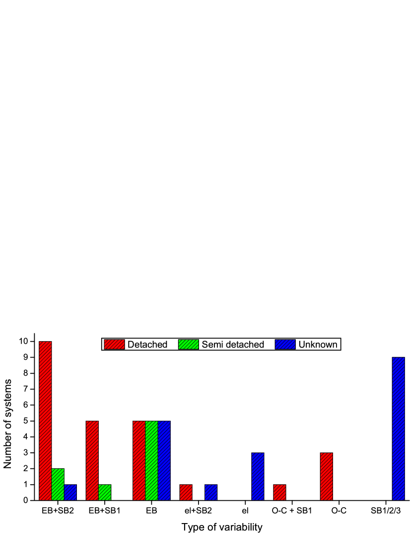
Figure 1: Demographics of the published cases of binaries with a $\delta$ Scuti component observed by the $Kepler$ and $K2$ missions according to their Roche geometry and type of variability.

MKR02 introduced for first time the term ‘$oEA\leavevmode\nobreak\ stars$’ (oscillating eclipsing binaries of Algol type) for characterizing the EBs with a $\delta$ Scuti mass accretor component of (B)A-F spectral type. The influence of mass accretion to the pulsational behaviour is one of the major questions of this particular topic of Asteroseismology and up to date there has been a lot discussion about it (e.g. TKA09; MKR18; BOW19). SOY06a announced the first connection between orbital ($P_{\rm orb}$) and dominant pulsation ($P_{\rm pul}$) periods for systems hosting a $\delta$ Scuti member. LIA12, after a six year observational survey, published a catalogue including 74 cases and updated correlations between fundamental parameters. ZHA13 made the first theoretical attempt for the $P_{\rm pul}-P_{\rm orb}$ correlation. LIAN15; LIAN16 noticed for the first time a possible boundary between $P_{\rm pul}-P_{\rm orb}$ beyond that these two quantities can be considered uncorrelated ($P_{\rm orb}\sim 13$ d). LIAN17 published the most complete catalogue for these systems to date (available online), which also includes updated correlations between fundamental parameters according to the geometrical status of the systems and the accuracy of their absolute parameters. A few months later, KAH17 almost doubled the threshold of $P_{\rm orb}$ by taking into account only the eclipsing systems. MUR18 published a review for binaries with pulsating components including also those with $\delta$ Scuti members. QIA18, using the LAMOST spectra of more than 760 $\delta$ Scuti stars, found that 88 of them are possibly members of binary or multiple systems.

$Kepler$ (BOR10; KOC10) and $K2$ (HOW14) missions are fairly considered as a benchmark for asteroseismology, although the first one was designed for exoplanet transits. They have offered a great amount of high accuracy data (order of tenths of mmag) allowing the detection of extremely low amplitude frequencies (order of a few $\upmu$mag; MUR13; BOW18). Moreover, the continuous recording of the targets eliminates the alias effects that are produced from the ground-based nightly-operated telescopes (BRE00). The time resolutions (short cadence $\sim 1$ min; long cadence $\sim 30$ min) of these space missions are extremely useful for the study of both EBs and short and long period pulsating stars. The easy access on the publicly available data from the $Kepler$ mission provided the means for astronomers to work at the same time in different topics. Especially for the EBs, a database hosting all the identified cases, namely ‘$Kepler$ Eclipsing Binary Catalog’ ($KEBC$, PRS11), has been developed and provides the detrended data and preliminary information (e.g. ephemerides, magnitudes, temperatures) for a few thousands of EBs.

The catalogue of LIAN17 includes 17 cases of $Kepler$ EBs with a $\delta$ Scuti component. However, today, this sample has been tripled. In particular, up to date, there have been published in total eight oEA stars, 25 detached systems, and 19 systems with unclassified Roche geometry. All these systems are listed in Table 1 along with their type of variability ($ToV$) and a corresponding reference, while their demographics are shown in Fig. 1. For the majority of these systems (i.e. the eclipsing and the ellipsoidal cases), the absolute parameters of the pulsating component(s) have been calculated using either LCs only or both LCs and RVs.

The present paper is a continuation of the systematic study on EBs with a $\delta$ Scuti component (see also LIA09; LIA13; LIA14; LIAN16; LIA17; LIA18) and aims to enrich the current sample of this kind of systems. Preliminary results have been published for KIC 10686876 (LIAN17), regarding its dominant pulsational frequencies, and together with KIC 04851217 were selected for detailed analyses for first time. The selected sample of binaries consists the $\sim 2.7\%$ of the 73 currently known detached binaries with a $\delta$ Scuti component (LIAN17, and subsequent individual publications as given in Table LABEL:tab:DEBsUPD) and the $\sim 4.9\%$ of those with $P_{\rm orb}<13$ days. Moreover, the present sample increases the sample of such systems observed by $Kepler$ (i.e. with detailed asteroseismic modeling) by $\sim 10.5\%$.

The results from the personal ground based spectroscopic observations, which allowed the estimation of the spectral types of the primary components of both studied systems, are given in Section 3. Section 4 includes the combined analysis of the $Kepler$ LCs and the spectroscopic data, which results in accurate modelings and estimations of the absolute parameters of the components of these systems. The further analyses of the LCs residuals, using Fourier transformation techniques, and the pulsational characteristics of the $\delta$ Scuti stars are presented in Section 5. The evolutionary status and the properties of the pulsating components of these systems are discussed and compared with other similar ones in Section LABEL:sec:Evol. Discussion, summary and conclusions are presented in Section LABEL:sec:Dis.

2 History of the selected systems

2.1 KIC 04851217

This system (HD 225524) has a period of $\sim 2.47$ d and a slightly eccentric orbit. Its first reference can be found in the Henry Draper extension catalogue (CAN36). Its first LC was obtained by HAR04 during the HATNET Variability Survey, while it was also observed by the ASAS survey (PIG09). ARM14 estimated the temperature of the system as 7022 K, while spectra obtained by LAMOST survey classified it between A5IV-A9V spectral types (GRA16; FRA16; QIA18). GIE15 calculated through an ETV analysis that the orbital period of the system increases with a rate $\sim 1.71\times 10^{-6}$ yr${}^{-1}$. RVs for both components have been obtained by MAT17 and HEL19. In the latter work, the masses of the components were calculated based also on the $Kepler$ LCs.

2.2 KIC 10686876

KIC 10686876 (TYC 3562-961-1) has an orbital period of $\sim 2.62$ d. Its first LC was obtained by the Trans-atlantic exoplanet survey (TrES; DEV08), while its temperature has been determined in the range 7944-8167 K (SLA11; CHR12; HUB14). GIE15, ZAS15, and BOR16 performed ETV analysis of the system and found a long term periodic term, which was attributed to the existence of a tertiary component. ZAS15 determined the period of the third body as $\sim 6.7$ yr and its mass function as $f$($m_{3}$)=0.021 $M_{\sun}$. In the same study, a preliminary LC modeling was also performed assuming a mass ratio of 1, resulting in a third light contribution of $\sim 5\%$. DAV16 listed it among the $Kepler$ systems exhibiting flare activity. LIAN17 included the system in their catalogue, mentioning also the dominant frequency of its $\delta$ Scuti component (21.02 d${}^{-1}$). MAT17 performed spectroscopic observations and measured the RVs of the primary component ($K_{1}$=67 km s${}^{-1}$).

3 Ground based Spectroscopy

The spectroscopic observations aimed to derive the spectral types of the primary components of the selected systems. The spectra of the KIC targets were obtained with the 2.3 m Ritchey-Cretien ‘Aristarchos’ telescope at Helmos Observatory in Greece in August and October 2016. The Aristarchos Transient Spectrometer (ATS) instrument (BOU04) using the low resolution grating (600 lines mm${}^{-1}$) was employed for the observations. This set-up provided a resolution of $\sim 3.2$ Å pixel${}^{-1}$ and a spectral coverage between approximately 4000-7260 Å. The spectral classification is based on a spectral line correlation technique between the spectra of the variables and standard stars, which were observed with the same set-up. In Table 2 are listed: The name of the system (KIC), the dates of observations, the exposure time used (E.T.), and the orbital phase of the system when the spectrum was obtained ($\Phi_{\rm orb}$). All spectra were calibrated (bias, dark, flat-field corrections) using the MaxIm DL software. The data reduction (wavelength calibration, cosmic rays removal, spectra normalization, sky background removal) was made with the RaVeRe v.2.2c software (NEL09).

The correlation method was presented in detail in LIA17, but is described here also in brief. The Balmer and the strong metallic lines between 4000-6800 Å were used for the comparison between the spectra of the KIC systems and the standards. The differences of spectral line depths between each standard star and the variables derive sums of squared residuals in each case, with the least squares sums to indicate the best fit. This method works very well in cases of binaries with large luminosity difference between the components, where the primary star dominates the total spectrum. However, in order to check possible contribution of the secondaries to the observed spectra, which would lead to an underestimation of the temperatures of the primary stars, another method was applied. Specifically, using the standard stars spectra, all possible combinations (i.e. combined spectra; sum of spectra) between spectral types A, F, G, and K were calculated. Moreover, for each spectra combination, the individual spectra were given weights, that are related to the light contribution of the components. The starting value for the contribution of the primary component was 0.5 and the step was 0.05. For each spectra combination, ten sub-combinations with different light contributions of the components were calculated. Each combined spectrum was compared with those of the variables deriving sums of squared residuals. Similarly to the direct comparison method, the least squares sums lead to the best match.

The light contribution of the primary of KIC 10686876 was found more than $95\%$, hence, its spectrum was compared directly with those of the standards. The components of KIC 04851217 were found to contribute almost equally to the observed spectrum, and, moreover, to be of the same spectral type. Therefore, practically, the combined spectrum was the same with that of a single star. The sum of squared residuals against the spectral type for these systems is plotted in Fig. 2. The best fit for the spectrum of KIC 04851217 was found with that of an A6V standard star, and that of KIC 10686876 with an A5V standard star. The spectra of both systems along with those of best-fit standard stars are given in Fig. 3. Table 2 includes also the spectral classification of the primary component of each system and the corresponding temperature values ($T_{\rm eff}$) according to the relations between effective temperatures and spectral types of COX00. A formal error of one sub-class is adopted and is propagated also in the temperature determination. The present results come in very good agreement with those of previous studies within the error ranges (see Sections 2.1-2.2).

Table 2: Spectroscopic observations log and results for the primary components of the studied systems. The errors are given in parentheses alongside values and correspond to the last digit(s).

KIC No	Date	E.T.	$\Phi_{\rm orb}$	Spectral	$T_{\rm eff}$
		(min)		type	(K)
04851217	17/8/16	10	0.67	A6V	8000(250)
10686876	16/8/16	10	0.22	A5V	8200(250)

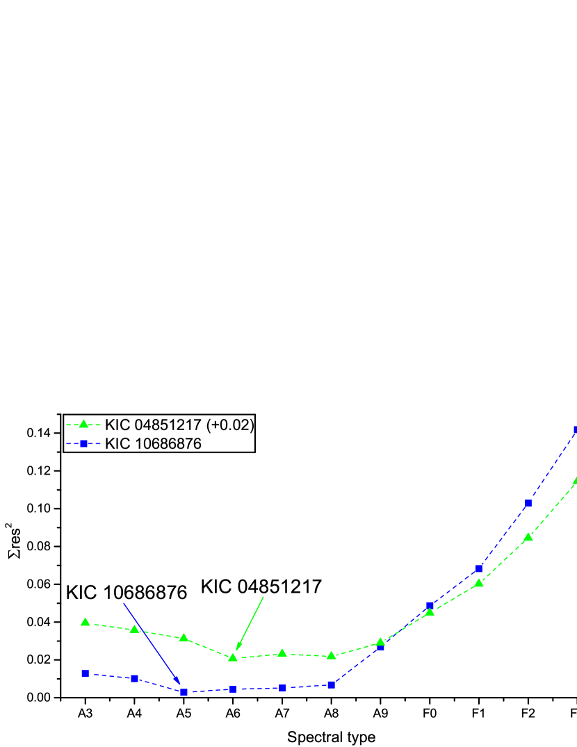
Figure 2: Spectral type-search plots for KIC 04851217 and KIC 10686876. The points of KIC 04851217 are shifted vertically for better viewing. The arrows show the adopted spectral type for the primary component of each system. The comparison is shown only between A3-F3 spectral types due to scaling reasons.

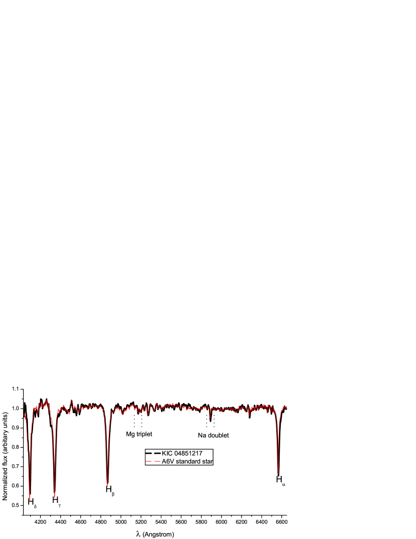
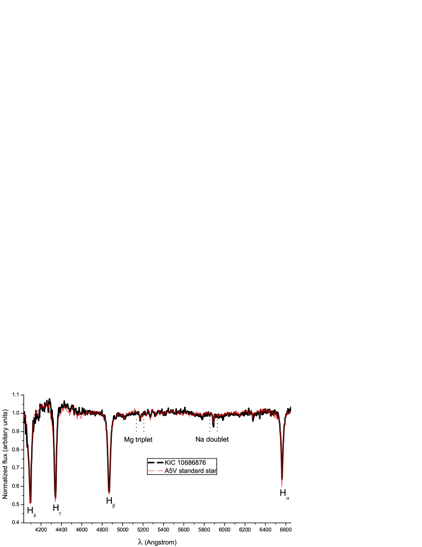
Figure 3: Comparison spectra of the studied systems (black lines) and standard stars (red lines) with the closest spectral types. The Balmer and some strong metallic lines are also indicated.

4 Light curve modelling and absolute parameters calculation

The selected systems were observed during many quarters of the $Kepler$ mission in long cadence mode. Additionally, both of them were also observed in short cadence mode during two or more quarters. Given that the primary objective of this work is the asteroseismic analysis of the pulsating stars of these systems (i.e. derivation of their oscillation frequencies and mode identification), only the short cadence data (downloaded from the $KEBC$; PRS11) were used for the subsequent analyses. The log of observations is given in Table 3, which includes: The level of light contamination ($light\leavevmode\nobreak\ contam.$), the total points, the number of days that data cover, and the number of the fully covered LCs. For both systems, the total covering time of observations is more than 1.8 years, which can be considered extremely sufficient for the study of short-period pulsations (i.e. order of hours) and more than enough for LC modelling. The short cadence $Kepler$ data of approximately 40 days of observations for each system are plotted in Fig. 4. The phases and the flux to magnitude conversions of both systems were calculated using the ephemerides ($T_{0},P_{\rm orb}$) and the $K_{\rm p}$ magnitudes, respectively, as given in $KEBC$ (PRS11, see also Table 4).

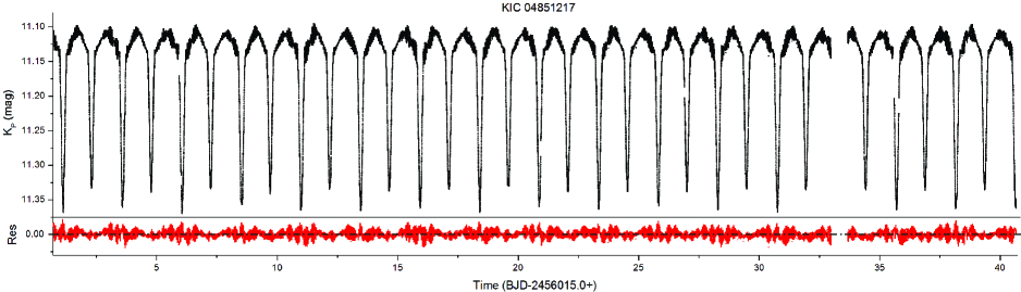
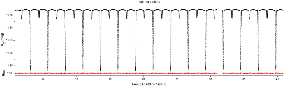
Figure 4: Short cadence LCs (black points) for the studied systems and their residuals (red points) after the subtraction of the LC models. The plotted data concern only 40 days of observations, while the rest are not shown for scaling reasons.

Table 3: Log of short cadence observations from the $Kepler$ mission for the studied systems.

KIC	Short cadence	$light\leavevmode\nobreak\ contam.$	Points	days	LCs
	quarter	($\times 10^{-3}$)	($\times 10^{5}$)
04851217	2, 4, 9, 13, 15-17	3	6.21	1360	164
10686876	3, 10	17	1.70	677	46

The LCs analyses were made with the PHOEBE v.0.29d software (PRS05) that is based on the 2003 version of the Wilson-Devinney code (WIL71; WIL79; WIL90). Temperatures of the primaries were assigned values derived from the present spectral classification (see Section 3 and Table 2) and were kept fixed during the analysis, while the temperatures of the secondaries $T_{2}$ were adjusted. Initially, for both systems, the albedos, $A_{1}$ and $A_{2}$, and gravity darkening coefficients, $g_{1}$ and $g_{2}$, were given values according to the spectral types of the components (RUC69; ZEI24; LUC67). The (linear) limb darkening coefficients, $x_{1}$ and $x_{2}$, were taken from the tables of HAM93. The synchronicity parameters $F_{1}$ and $F_{2}$ were initially left free, but since they did not show any significant change during the iterations, they were given a value of 1 (tidal locking). The dimensionless potentials $\Omega_{1}$ and $\Omega_{2}$, the fractional luminosity of the primary component $L_{1}$, and the inclination of the system $i$ were set as adjustable parameters. The third light contribution $l_{3}$ was also set as adjustable parameter for the system which either has significant light contamination or there is information about possible tertiary component. For the present sample of systems, $l_{3}$ was taken into account only for KIC 10686876 (see Section 4.2 for details), while for KIC 04851217 the light contamination is negligible ($<$0.3%). At this point, it should to be noted that since the CCD sensors of $Kepler$ have effective wavelength response between approx. 410-910 nm with a peak at $\sim 588$ nm, the $R$ filter (Bessell photometric system–range between 550-870 nm and with a transmittance peak at 597 nm) was selected as the best representative for the filter depended parameters (i.e. $x$ and $L$).

As described in the previous works (LIA17; LIA18), the analyses of EBs observed by $Kepler$ LCs need some special attention due to light variations between successive LCs. Therefore, in order to avoid a super simplified model including all data points folded into the $P_{\rm orb}$, the method of one model per LC (using normal points) or one model per a group of successive LCs folded into the $P_{\rm orb}$ was followed. The reasons for this are: a) the brightness changes from cycle to cycle due to magnetic activity and b) the asymmetries due to the pulsations (i.e. superimpositions or damping of the various frequency modes). It should be noticed that the derived LC residuals should exclude as much as possible the proximity and other stellar effects (e.g. magnetic activity) in order to perform subsequently an accurate frequency analysis (see next Section). The one model per LC or per a group of successive LCs technique provides also the means to derive more realistic errors for the adjusted parameters and minimize the widely known ‘unrealistic’ error estimation of PHOEBE. The final LC model of a system includes the average values of the respective parameters from all the individual models, while their errors are the standard deviations of them. The LC analyses were applied in modes 2 (detached system), 4 (semi-detached system with the primary component filling its Roche lobe) and 5 (conventional semi-detached binary). Neither of these systems could converge in any semi-detached mode, therefore, both of them can be plausibly considered as detached EBs. The method described above is general and additional information for the analysis of each system is given in the following subsections.

Table 4: Modeling and absolute parameters for the studied systems. The errors are given in parentheses alongside values and correspond to the last digit(s).

System:	KIC 04851217	KIC 10686876
	System parameters
$K_{\rm p}^{(1)}$ (mag)	11.11	11.73
$T_{0}^{(1)}$ (BJD)	2454953.90(5)	2454953.95(3)
$P_{\rm orb}^{(1)}$ (d)	2.470280(4)	2.618427(4)
$q$ ($m_{2}$/$m_{1}$)	1.14(4)	0.44(1)
$i$ ($\degr$)	76.7(1)	86.4(1)
$e$	0.036(1)	-
$\omega$ ($\degr$)	2.64(1)	-
	Components parameters
$T_{1}$ (K)	8000(250)${}^{(2)}$	8200(250)${}^{(2)}$
$T_{2}$ (K)	7890(98)	4740(115)
$\Omega_{1}$	5.94(1)	6.14(1)
$\Omega_{2}$	6.26(1)	7.00(8)
$K_{1}$ (km s${}^{-1}$)	131(2.6)${}^{(3)}$	67(2)${}^{(4)}$
$K_{2}$ (km s${}^{-1}$)	114.6(2.7)${}^{(3)}$	-
$A_{1}$	1	1
$A_{2}$	1	1
$g_{1}$	1	1
$g_{2}$	1	0.32
$x_{1}$	0.439	0.377
$x_{2}$	0.444	0.500
$L_{1}$/$L_{\rm T}$	0.585(2)	0.948(1)
$L_{2}$/$L_{\rm T}$	0.415(1)	0.023(2)
$L_{3}$/$L_{\rm T}$	-	0.029(1)
$r_{1,\leavevmode\nobreak\ \rm pole}$	0.209(1)	0.175(1)
$r_{2,\leavevmode\nobreak\ \rm pole}$	0.217(1)	0.077(1)
$r_{1,\leavevmode\nobreak\ \rm point}$	0.216(1)	0.177(1)
$r_{2,\leavevmode\nobreak\ \rm point}$	0.223(1)	0.077(1)
$r_{1,\leavevmode\nobreak\ \rm side}$	0.212(1)	0.176(1)
$r_{2,\leavevmode\nobreak\ \rm side}$	0.219(1)	0.077(1)
$r_{1,\leavevmode\nobreak\ \rm back}$	0.215(1)	0.177(1)
$r_{2,\leavevmode\nobreak\ \rm back}$	0.222(1)	0.077(1)
	Absolute parameters
$M_{1}\leavevmode\nobreak\$($M_{\sun}$)	1.92(10)	2.0(2)
$M_{2}\leavevmode\nobreak\$($M_{\sun}$)	2.19(18)	0.88(9)
$R_{1}\leavevmode\nobreak\$($R_{\sun}$)	2.61(5)	2.00(7)
$R_{2}\leavevmode\nobreak\$($R_{\sun}$)	2.68(5)	0.88(9)
$L_{1}\leavevmode\nobreak\$($L_{\sun}$)	25(3)	16(2)
$L_{2}\leavevmode\nobreak\$($L_{\sun}$)	25(3)	0.3(1)
$\log g_{1}$ (cm s${}^{-2}$)	3.89(3)	4.14(5)
$\log g_{2}$ (cm s${}^{-2}$)	3.92(4)	4.50(10)
$a_{1}$ ($R_{\sun}$)	6.6(1)	3.5(1)
$a_{2}$ ($R_{\sun}$)	5.7(1)	7.9(3)
$M_{\rm bol,\leavevmode\nobreak\ 1}$ (mag)	1.26(6)	1.73(8)
$M_{\rm bol,\leavevmode\nobreak\ 2}$ (mag)	1.26(4)	5.9(1)

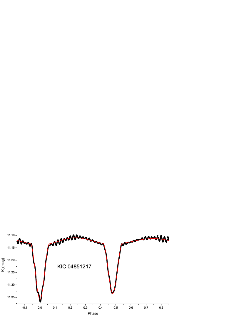
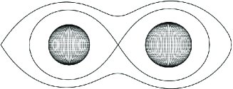
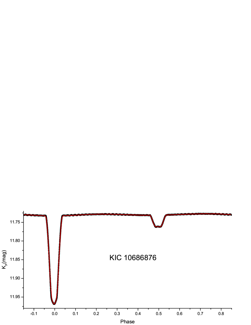
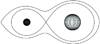
Figure 5: Theoretical (solid lines) over observed (points) LCs (one cycle) and two-dimensional representations of the Roche geometry at orbital phase 0.75 for the studied systems.

4.1 KIC 04851217

For this system there are two spectroscopic studies regarding the RVs of its components in the literature. As mentioned in Section 2.1, MAT17 calculated the amplitudes of the RVs as $K_{1}$=$115$ km s${}^{-1}$ and $K_{2}$=107 km s${}^{-1}$, for the primary and the secondary components, respectively, while HEL19 found $K_{1}$=131 km s${}^{-1}$ and $K_{2}$=115 km s${}^{-1}$. In the latter study, the authors, additionally to their personal observations, they also used data from the Trans-atlantic Exoplanet Survey (TrES; ALO04) and Apache Point Observatory Galactic Evolution Experiment (APOGEE; MAJ17). Therefore, that work is considered as more complete and reliable, given the larger data set used, hence, their results were adopted for the present study. According to these $K_{1}$ and $K_{2}$ values, a mass ratio ($q$) of 1.14$\pm$0.04 was calculated. This value was initially assigned in PHOEBE, but during the iterations it was left free to adjust inside its error range. Moreover, due to the displacement of the secondary minimum from the phase 0.5, the eccentricity $e$ and the argument of periastron $\omega$ were also left free to adjust. Given that no brightness changes due to magnetic activity were detected, one model per approximately six successive LCs folded into the $P_{\rm orb}$ was derived, resulting in total in 27 individual LC models.

4.2 KIC 10686876

The analysis of this system was revealed as the most complicated in comparison with the previous one. First of all, using the findings of MAT17, who measured the RV1 and calculated $K_{1}$=67$\pm$2 km s${}^{-1}$, and according to the present results about the spectral type of the primary component (A5V), the analysis was constrained in the range $0.4<q<0.5$ (c.f. WAN19). In this regime, the expected mass of the primary ranges between 1.5-2.5 $M_{\sun}$. However, following exactly the same method likely for the previous EB regarding the fixed parameters and by adopting spots to fit the asymmetries, no sufficient solution was found in this $q$ range. Therefore, the iterations continued beyond this range and the best solution was found for $q\sim 0.28$. The LC solution for this $q$ value derives $M_{1}$=6 $M_{\sun}$, $M_{2}$=1.72 $M_{\sun}$ and $T_{2}\sim 4800$ K. Although, that was the best numerical solution based on the sum of squared residuals, however, there was not any physical meaning regarding the parameters of the components. Therefore, the modelling started again in the $q$ range 0.4-0.5, with the difference that $A_{2}$ was set to 1, which can be interpreted as reflection from the much hotter primary component. KIC 10686876 presents significant brightness changes due to magnetic activity (listed also as system exhibiting flare activity by DAV16), hence, hot and cool spots on the surface of the secondary component were adopted. In addition, $l_{3}$ was also adjusted because the system a) has a light contamination of 1.7$\%$ (Table 3) and b) possibly hosts a tertiary component (GIE15; ZAS15; BOR16).

The LCs modeling results for both systems are given in the upper and middle parts of Table 4. Examples of LC modeling and the Roche geometry of each system are illustrated in Fig. 5.The LCs residuals after the subtraction of the individual models are shown below the observed LCs in Fig. 4. In addition, the parameters of the spots for each LC (cycle) of KIC 10686876 (Table LABEL:tab:spots) are given in appendix LABEL:sec:App2. The variations of the parameters of the spots over time and various 2D representations showing the positions of the spots on the surface of the secondary component for two different dates of observations are plotted in Fig. LABEL:fig:spotKIC106.

Using the RVs curves for these systems, the absolute parameters of their components can be fairly formed. However, given that for KIC 10686876 only the RV1 has been measured, the mass of its primary was inferred from its spectral type according to the spectral type-mass correlations of COX00 for main-sequence stars. A fair mass error value of 10$\%$ was also adopted. The secondary’s mass follows from the determined mass ratio. The semi-major axes $a$, which fix the absolute mean radii, can then be derived from Kepler’s third law. The luminosities ($L$), the gravity acceleration ($\log g$), and the bolometric magnitudes values ($M_{\rm bol}$) were calculated using the standard definitions. The absolute parameters were calculated with the software AbsParEB (LIA15) and they are given in the lower part of Table 4.

5 Pulsation frequencies analysis

The results from spectroscopy and LCs modelling (Sections 3 and 4) indicate that for KIC 10686876 only the primary component fits well to the profiles of the $\delta$ Scuti type stars (i.e. mass and temperature). On the other hand, the components of KIC 04851217 show similar physical properties, therefore, additional search was needed in order to reveal the pulsating component (see Section LABEL:sec:KIC048freqdetails). The pulsation frequencies analysis was performed with the software PERIOD04 v.1.2 (LEN05) that is based on classical Fourier analysis. The typical frequencies range of $\delta$ Scuti stars is 4-80 d${}^{-1}$ (BRE00; BOW18), hence, the search should had been made for this range. However, an extensive range between 0-80 d${}^{-1}$ was selected for the search, since $\delta$ Scuti stars in binary systems may also present $g$-mode pulsations that are connected to their $P_{\rm orb}$ or present hybrid behaviour of $\gamma$ Doradus- $\delta$ Scuti type. For these analyses, the LCs residuals of each system (i.e. after the subtraction of the LCs models) were used (Fig. 4). A 4$\upsigma$ limit (S/N$=4$; recommended by LEN05) regarding the reliability of the detected frequencies was adopted. Hence, after the first frequency computation the residuals were subsequently pre-whitened for the next one until the detected frequency had S/N$\sim$4. The Nyquist frequency and the frequency resolution according to the Rayleigh-Criterion (i.e. 1/$T$, where $T$ is the observations time range in days) are 733 d${}^{-1}$ and 0.0007 d${}^{-1}$ for KIC 04851217, and 732 d${}^{-1}$ and 0.001 d${}^{-1}$ for KIC 10686876, respectively.

After the frequencies search, the relation of BRE00 was used for the calculation of the pulsation constants ($Q$) of the independent frequencies:

$$\log Q=-\log f+0.5\log g+0.1M_{\rm bol}+\log T_{\rm eff}-6.456,\\$$ (1)

where $f$ is the frequency of the pulsation mode, while $\log g$, $M_{\rm bol}$, and $T_{\rm eff}$ denote the standard quantities (see Section 4). Subsequently, using the pulsation constant - density relation:

$$Q=f_{\rm dom}^{-1}\sqrt{\rho_{\rm pul}/\rho_{\sun}},\\$$ (2)

where $f_{\rm dom}$ is the frequency of the dominant pulsation mode (i.e. that with the largest amplitude), the density of the pulsator $\rho_{\rm pul}$ in solar units was also calculated. The results for the aforementioned quantities for each pulsator are given in Table 5. It should be noticed that the $Q$ values for all modes of both pulsators, except one for KIC 10686876, lie within the typical range of $\delta$ Scuti stars (i.e. $0.015<Q<0.035$; BRE00). Moreover, it should to be noted that the majority of $\delta$ Scuti stars exhibit intrinsic amplitude modulation (BOW16; BAR20), hence, $f_{\rm dom}$ may differ from time to time. Therefore, the present calculated densities might be not that accurate. However, they can be considered as rather representatives, since the respective calculations for the other pulsation modes for both systems yield very similar values.

The mode identification (i.e. $l$-degrees and the type of each oscillation) was made using the theoretical MAD models for $\delta$ Scuti stars (MON07) in the FAMIAS software v.1.01 (ZIM08). These models have a grid step 0.05-0.1 $M_{\sun}$ in the mass range 1.6-2.2 $M_{\sun}$, which is sufficient for the studied systems. The models ($l$-degrees) of the detected independent frequencies that corresponded to the parameters ($\log g$, $M$, and $T_{\rm eff}$) of the pulsators were adopted as the most probable oscillation modes. Moreover, $P_{\rm pul}$/$P_{\rm orb}$ ratios for all frequencies were also calculated and found below 0.07, except for $f_{7}$ of KIC 10686876, indicating that they are probably of $p$-mode type (ZHA13).

The results for the independent frequencies for both systems as well as their mode identification are given also in Table 5. The frequency values $f_{\rm i}$ with the respective amplitudes $A$, phases $\Phi$, and S/N are listed along with the $Q$, $\rho_{\rm pul}$, $P_{\rm pul}$/$P_{\rm orb}$, $l$-degrees, and modes. Similarly, the parameters of the dependent (combination) frequencies are given in Tables LABEL:tab:DepFreqKIC048-LABEL:tab:DepFreqKIC106 in appendix LABEL:sec:App1. The periodograms of the systems, on which the independent frequencies and the stronger frequencies that are connected to their $P_{\rm orb}$ are indicated, as well as the distributions of the frequencies are given in Fig. LABEL:fig:FS. Examples of the Fourier fitting on the observed points for both systems are given in Fig. LABEL:fig:FF. Comments and information for the individual analysis of each system are given in the following subsections.

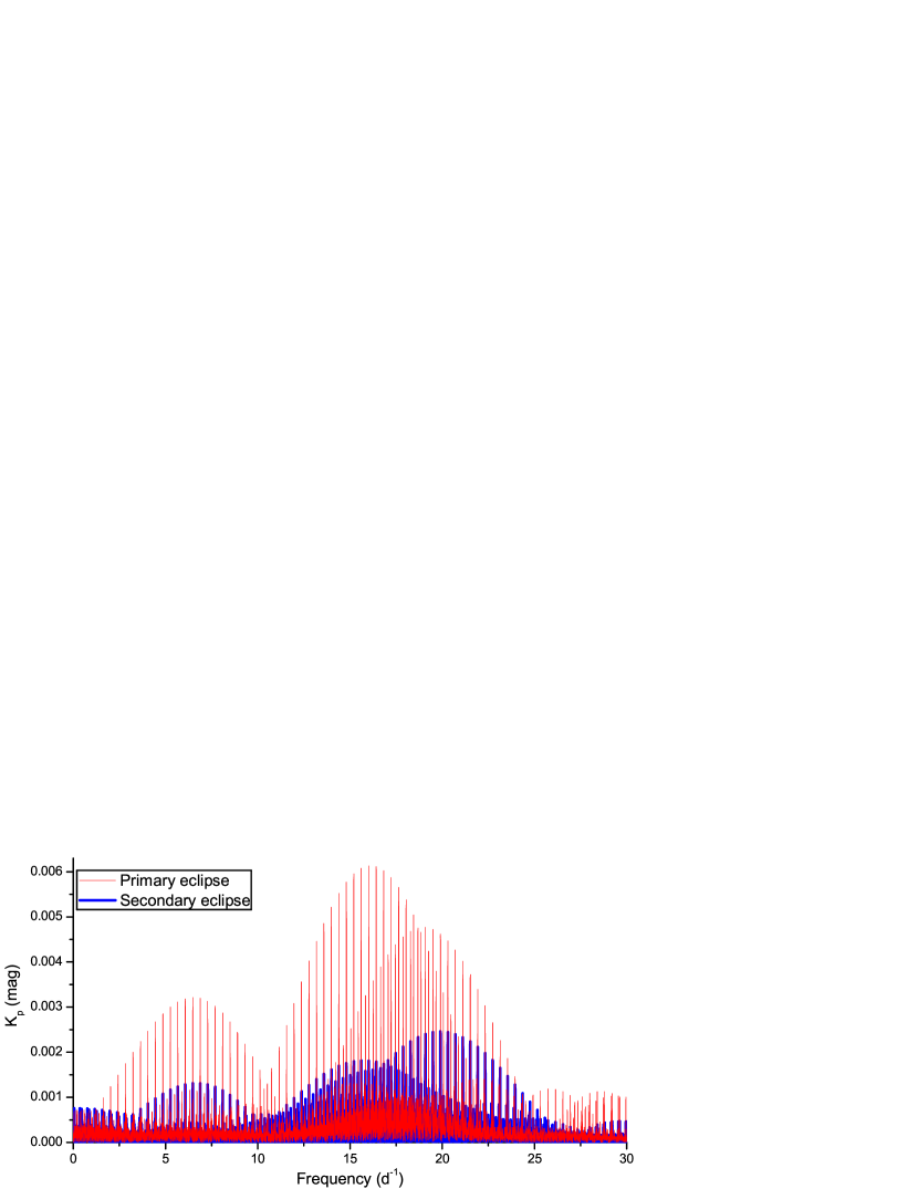
Figure 6: Periodograms for the data during the eclipses (red=primary; blue=secondary) of KIC 04851217. The amplitudes of the frequencies during the primary eclipse are almost tripled indicating that the pulsating member of the system is the secondary component.

Table 5: Independent oscillation frequencies and mode identification for the pulsating components of both systems. The errors are given in parentheses alongside values and correspond to the last digit(s).

$i$	$f_{\rm i}$	$A$	$\Phi$	S/N	$Q$	$\rho_{\rm pul}$	$P_{\rm pul}$/	$l$-degree	Pulsation mode
	(d-1)	(mmag)	(°)		(d)	(ρ☉)
KIC04851217
1	19.092413(1)	3.765(7)	310.8(1)	205.8	0.018