On the Resolution Probability of Conditional and Unconditional Maximum Likelihood DoA Estimation

Abstract

After decades of research in Direction of Arrival (DoA) estimation, today Maximum Likelihood (ML) algorithms still provide the best performance in terms of resolution capabilities. At the cost of a multidimensional search, ML algorithms achieve a significant reduction of the outlier production mechanism in the threshold region, where the number of snapshots per antenna and/or the signal to noise ratio (SNR) are low. The objective of this paper is to characterize the resolution capabilities of ML algorithms in the threshold region. Both conditional and unconditional versions of the ML algorithms are investigated in the asymptotic regime where both the number of antennas and the number of snapshots are large but comparable in magnitude. By using random matrix theory techniques, the finite dimensional distributions of both cost functions are shown to be Gaussian distributed in this asymptotic regime, and a closed form expression of the corresponding asymptotic covariance matrices is provided. These results allow to characterize the asymptotic behavior of the resolution probability, which is defined as the probability that the cost function evaluated at the true DoAs is smaller than the values that it takes at the positions of the other asymptotic local minima.

I Introduction

The determination of the direction of arrival (DoA) of one or multiple far-field sources continues to be a highly relevant problem in multiple fields, such as radar, sonar, seismology or radioastronomy. Among all the DoA determination methods available today, classical Maximum Likelihood (ML) procedures remain to be the ones that offer the best performance in terms of both precision and spatial resolution. The extraordinary performance of ML methods comes at the expense of an increased computational complexity, since they require a non-linear multi-dimensional search instead of a one-dimensional one (as it is the case in subspace-based algorithms). However, ML methods still represent the only valid alternative in challenging scenarios with closely located and/or highly correlated sources. They are also the most attractive solution in offline processing applications.

Several alternatives have been proposed in the literature in order to alleviate the high computational complexity associated with the non-linear multidimensional search of ML methods. One can differentiate between algorithms that try to simplify the local search procedure and algorithms that aim to simplify the global search. Among the first group, we can include the alternating projection method [1], the IQML algorithm for Uniform Linear Arrays (ULA) [2], some methods based on large sample volume approximations of the ML objective function (such as MODE [3] or related alternatives [4, 5]), and some recently proposed approximate ML methods for the specific case where only two closely spaced sources are present in the scenario [6, 7]. All these methods achieve a significant reduction of the computational complexity at the expense of a certain performance loss, caused by the fact that the ML objective function is in fact approximated. The second family of ML-based DoA detection algorithms are aimed at simplifying the global multidimensional search, avoiding the computational burden associated with an evaluation of the ML objective function in a uniform multidimensional fine grid. One may include here genetic algorithms for global search [8, 9], or two-stage methods that first select a set of candidate DoAs with simpler one-dimensional search methods and then refine these initial estimations by a multidimensional ML search procedure [10, 11]. The aim of all these global search methods is to avoid convergence to a local extremum of the ML objective function while avoiding the need to evaluate this function at a high number of points in the multi-dimensional grid.

One must point out that there exist two alternative ML DoA estimation procedures with different objective functions, depending on whether the signals are modeled as stochastic or as unknown deterministic parameters. The Unconditional ML (UML) method is based on the assumption that the source signals are temporally white Gaussian random variables [12, 13], whereas the Conditional ML (CML) method simply treats them as unknown deterministic parameters that need to be estimated. It was early recognized [14] that the UML method asymptotically outperforms CML when the number of samples tends to infinity for a fixed array dimension. In fact, it was shown in [15] that, contrary to UML, the CML method is statistically inefficient, in the sense that the algorithm does not achieve the Cramér-Rao Bound (CRB) corresponding to the deterministic signal assumption. This effect is caused by the fact that the total number of parameters that need to be estimated by the CML method increases with the sample size, whereas this is not the case in the UML algorithm. On the other hand, it was demonstrated in [16] that CML and UML are in fact equivalent at large signal to noise ratio (SNR), meaning that the difference between their estimates converges to zero in probability, even for finite values of the sample volume.

All of the above performance results for CML and UML are only valid in the small error regime, that is when the estimated DoAs are very close to the true ones, either because of a relatively large sample volume with respect to the array dimension [14] or a relatively low noise power level with respect to the source signals [17, 16]. Unfortunately, none of the above insights carry over to the more relevant case where the number of samples is comparable to the array dimension and the SNR is moderately low. Note that this is precisely the regime where ML offers the main advantages with respect to other one-dimensional DoA estimation techniques, such as more conventional subspace based approaches. The main objective of this paper will be the performance characterization of the CML and UML techniques in this “threshold region”, whereby both the number of samples per antenna and the SNR take moderate values. This region is typically characterized by a systematic appearance of outliers in the DoA estimates, which are mainly caused by the incapability of resolving closely spaced sources.

Unfortunately, the performance of CML and UML DoA estimation methods in this threshold region has received less attention in the literature. One of the most relevant contributions in this direction was the work by Athley in [18], which characterized the probability of resolving closely spaced sources for finite values of the sample size and SNR. Some additional insights into the problem were given in [19], where the outlier production mechanism was related to the asymptotic eigendecomposition of the observation covariance matrix. Recently, the approach in [18] has been used to study the resolution probability of both CML and UML in the multi-frequency case [20]. In this paper, we also follow the approach in [18] and characterize the resolution probability of these two ML methods by studying the stochastic behavior of the CML and UML objective functions under the assumption that the observations are Gaussian random variables. Our approach will be asymptotic in both the number of antennas and the number of samples, although we will always assume that both the SNR and the number of samples per antenna are finite and bounded quantities. In practice, this asymptotic regime models the situation where the number of antennas is of the same order of magnitude as the number of available snapshots.

The approach followed by Athley in [18] conforms to the classical Method of Interval Errors (MIE), which predicts the threshold region performance of estimation methods based on minimizing a certain cost function. This method has also been used in [21] to characterize the threshold performance of the Capon method and in [22] to study the threshold of the ML estimation method corresponding to one signal in spatially colored noise. The main idea is that the mean squared error (MSE) of the estimated parameters can be decomposed into a sum of two weighted terms, a local error term (the small-error variance), and an outlier term for global errors (outliers), that is

$$MSE=P_{res}MSE_{\text{small}}+(1-P_{res})MSE_{\text{large}}$$ (1)

where $MSE_{\text{small}}$ is the small error MSE (usually the Cramér-Rao Bound), $MSE_{\text{large}}$ is the large error MSE (typically approximated as the average MSE under a uniformly distributed parameter choice) and $P_{res}$ is the resolution probability. In order to characterize the resolution probability, the MIE identifies all the local minima of the asymptotic (deterministic) cost function. Clearly, only one of these local minima will be associated to the true value of the parameters (the global minimum, assuming consistency), whereas the rest will contain the typical values taken by outliers, which can all be associated to other local minima. The resolution probability is defined as the probability that the value of the cost function at the position of the deterministic global minima (true DoAs) is smaller than the values at the rest of the local ones. Observe that the global behavior of the random cost function is summarized as the behavior in a finite set of deterministic points.

The rest of the paper is structured as follows. Section II introduces the conditional and unconditional ML DoA estimation methods and presents the two main results of the paper, namely (i) almost sure convergence of the ML cost functions and (ii) convergence in law of the associated finite dimensional distributions. The proof of these two main results is given in Section III and Section IV respectively. Section V provides a numerical evaluation of the asymptotic probability of resolution that is established according to the results in Section II and finally Section VI concludes the paper.

II DoA ML Methods and Main Asymptotic Results

Let us denote by $\mathbf{y}(n)\in\mathbb{C}^{M\times 1}$ a column vector that contains the complex samples received by an array of $M$ elements at the $n$th time instant. This signal contains the contribution from $K<M$ far field sources with DoAs $\bar{\theta}=\left[\bar{\theta}(1),\ldots,\bar{\theta}(K)\right]^{T}$, so that we can express $\mathbf{y}(n)$ as

$$\mathbf{y}(n)=\mathbf{A}(\bar{\theta})\mathbf{s}(n)+\mathbf{n}(n).$$

In this expression, $\mathbf{s}(n)$ $\in\mathbb{C}^{K\times 1}\,$ is a column vector with the source signal samples, $\mathbf{A}(\bar{\theta})$ $\in\mathbb{C}^{M\times N}$ is a matrix that contains as columns the steering vectors corresponding to the different directions of arrival and $\mathbf{n}(n)\in\mathbb{C}^{M\times 1}$ is a column vector with background noise entries, assumed independent and identically distributed (i.i.d.) according to a circularly symmetric Gaussian law with with zero mean and unknown variance $\sigma^{2}$. Assume that $N$ different snapshots or realizations of $\mathbf{y}(n)$ are available, and denote $\mathbf{Y}=\left[\mathbf{y}(1),\ldots,\mathbf{y}(N)\right]$. As mentioned above, two different ML methods for the estimation of $\bar{\theta}$ can be derived depending on the nature of the signal vectors $\mathbf{s}(n)$. In both cases, the minimization is carried out in a multidimensional compact domain $\Theta_{K}\subset\mathbb{R}^{K}$ for which $\mathbf{A}(\theta)$ has full column rank, for example

$$\Theta_{K}=\{\theta_{1}<\ldots<\theta_{K},\theta_{k}\geq\theta_{k-1}+\varepsilon,\theta_{1}\geq-\pi+\varepsilon,\theta_{K}\leq\pi-\varepsilon\}$$ (2)

for some small $\varepsilon>0$.

II-A Conditional ML

In the conditional model, the signals are assumed to be deterministic unknown parameters, denoted by $\mathbf{S=}\left[\mathbf{s}(1),\ldots,\mathbf{s}(N)\right]$. The corresponding ML estimator is the minimizer of the normalized negative log-likelihood

$$L_{C}\left(\sigma^{2},\mathbf{S,}\theta\right)=M\log\sigma^{2}+\frac{1}{N\sigma^{2}}\left\|\mathbf{Y-A}(\theta)\mathbf{S}\right\|_{F}^{2}$$

where $\left\|\text{{\textperiodcentered}}\right\|_{F}$ is the Frobenius norm and where we constrain $\sigma^{2}>0$. The minimum is achieved at $\mathbf{\hat{S}(}\theta)=(\mathbf{A}^{H}(\theta)\mathbf{A}(\theta))^{-1}\mathbf{A}^{H}(\theta)\mathbf{Y}$ and, regardless of $\sigma^{2}$, the CML estimator of $\theta$ is obtained by minimizing the cost function $L_{C}(\sigma^{2},\mathbf{\hat{S}}(\theta)\mathbf{,}\theta)$ or, equivalently, the function

$$\hat{\eta}_{C}\left(\theta\right)=\frac{1}{M}\operatorname*{tr}\left[\mathbf{P}_{A}^{\perp}(\theta)\mathbf{\hat{R}}\right]$$ (3)

where $\mathbf{\hat{R}}$ is the sample covariance matrix, i.e. $\mathbf{\hat{R}}=\frac{1}{N}\mathbf{YY}^{H}$, and $\mathbf{P}_{A}^{\perp}(\theta)$ is the orthogonal projection matrix onto the null column space of $\mathbf{A}(\theta)$, namely $\mathbf{P}_{A}^{\perp}(\theta)=\mathbf{I}_{M}-\mathbf{P}_{A}(\theta)$, where

$$\mathbf{P}_{A}(\theta)=\mathbf{A}(\theta)\left(\mathbf{A}^{H}(\theta)\mathbf{A}(\theta)\right)^{-1}\mathbf{A}^{H}(\theta).$$

II-B Unconditional ML

The unconditional model assumes the signals $\mathbf{s}(n)$ are independent circularly symmetric Gaussian vectors with zero mean and unknown covariance matrix $\mathbf{P}_{s}=\mathbb{E}\left[\mathbf{s}(n)\mathbf{s}^{H}(n)\right]$. In this case, the ML estimator can be formulated as the minimizer of normalized negative log-likelihood

$$L_{U}\left(\mathbf{P}_{s},\sigma^{2},\theta\right)=\log\det\mathbf{R}\left(\mathbf{P}_{s},\sigma^{2},\theta\right)+\mathrm{tr}\left[\mathbf{R}^{-1}\left(\mathbf{P}_{s},\sigma^{2},\theta\right)\mathbf{\hat{R}}\right]$$

where here again $\mathbf{\hat{R}}$ is the sample covariance matrix defined above and where $\mathbf{R}\left(\mathbf{P}_{s},\sigma^{2},\theta\right)=\mathbf{\mathbf{A}}(\theta\mathbf{)P}_{s}\mathbf{A}^{H}(\theta)+\sigma^{2}\mathbf{I}_{M}$. The above minimization is carried with the constraints $\mathbf{P}_{s}\geq 0,$ $\sigma^{2}>0$ and $\theta\in\Theta_{K}$. The solution to the above optimization problem can be formulated as follows. Let us denote by $\hat{\alpha}_{1}(\theta\mathbf{)}\leq\ldots\leq\hat{\alpha}_{K}(\theta\mathbf{)}$ the eigenvalues of the $K\times K$ matrix $\mathbf{U}_{A}^{H}(\theta)\mathbf{\hat{R}\mathbf{U}}_{A}(\theta)$, where $\mathbf{U}_{A}(\theta)=\mathbf{A}(\theta)(\mathbf{A}^{H}(\theta)\mathbf{A}(\theta))^{-1/2}$ and let $\mathbf{\hat{q}}_{1}(\theta),\ldots,\mathbf{\hat{q}}_{K}(\theta)$ denote the associated eigenvectors. For $k=1,\ldots,K$, denote by $\hat{\Lambda}_{k}(\theta)$ a $k\times k$ diagonal matrix that contains the $k$ highest eigenvalues and let $\mathbf{\hat{Q}}_{k}(\theta)$ be defined as a $K\times k$ matrix that contains the associated eigenvectors, that is $\hat{\Lambda}_{k}(\theta)=\mathrm{diag}(\hat{\alpha}_{K-k+1}(\theta),\ldots,\hat{\alpha}_{K}(\theta))$ and $\mathbf{\hat{Q}}_{k}(\theta)=[\mathbf{\hat{q}}_{K-k+1}(\theta),\ldots,\mathbf{\hat{q}}_{K}(\theta)]$. Furthermore, we define $\hat{\sigma}_{k}^{2}(\theta)$ as

$$\hat{\sigma}_{k}^{2}(\theta)=\frac{1}{M-k}\mathrm{tr}\left[\mathbf{\hat{R}}\left(\mathbf{I}-\mathbf{U}_{A}(\theta)\mathbf{\hat{Q}}_{k}(\theta)\mathbf{\hat{Q}}_{k}^{H}(\theta)\mathbf{\mathbf{U}}_{A}^{H}(\theta)\right)\right].$$

Now, let $m$ denote the maximum integer such that $\hat{\Lambda}_{m}(\theta)>\hat{\sigma}_{m}^{2}(\theta)\mathbf{I}_{m}$. If there does not exist such an integer (meaning that $\hat{\alpha}_{K}(\theta\mathbf{)}<\hat{\sigma}_{1}^{2}(\theta)$) then the optimum is achieved at $\mathbf{P}_{s}=0$ and $\sigma^{2}=\frac{1}{M}\mathrm{tr}\mathbf{\hat{R}}$. Otherwise, the function $L_{U}(\mathbf{P}_{s},\sigma^{2},\theta)$ reaches its minimum at $\sigma^{2}=\hat{\sigma}_{m}^{2}(\theta)$ and $\mathbf{P}_{s}=\mathbf{\hat{P}}_{s}^{(m)}$, where

$$\mathbf{\hat{P}}_{s}^{(m)}=\left(\mathbf{A}^{H}(\theta)\mathbf{A}(\theta)\right)^{-1/2}\mathbf{\hat{Q}}_{m}(\theta)\left(\hat{\Lambda}_{m}(\theta)-\hat{\sigma}_{m}^{2}(\theta)\mathbf{I}_{m}\right)\mathbf{\hat{Q}}_{m}^{H}(\theta)\left(\mathbf{A}^{H}(\theta)\mathbf{A}(\theta)\right)^{-1/2}.$$

Furthermore, the corresponding negative log-likelihood takes the minimum value

$$L_{U}\left(\mathbf{\hat{P}}_{s}^{(m)},\hat{\sigma}_{m}^{2}(\theta),\theta\right)=\left(M-m\right)\log\hat{\sigma}_{m}^{2}(\theta)+\log\det\hat{\Lambda}_{m}(\theta)+M.$$

The UML estimator can therefore be obtained by exploring the above cost function over the domain $\Theta_{K}$. The problem here is that every time we need to evaluate the above expression at a particular $\theta$ we need to find the full eigendecomposition of the matrix $\mathbf{U}_{A}^{H}(\theta)\mathbf{\hat{R}\mathbf{U}}_{A}(\theta)$, so finding the true UML estimator is quite complex from the computational complexity. For this reason, typical implementations of the UML DoA estimator assume that $N>K$ and $\hat{\alpha}_{1}(\theta\mathbf{)}>\hat{\sigma}_{K}^{2}(\theta)$ [12, 13], implying that $m=K$ and turning the problem into the minimization of

$$\hat{\eta}_{U}\left(\theta\right)=\frac{M-K}{M}\log\hat{\sigma}_{K}^{2}(\theta)+\frac{1}{M}\log\det\left(\mathbf{U}_{A}^{H}(\theta)\mathbf{\hat{R}\mathbf{U}}_{A}(\theta)\right)$$ (4)

where

$$\hat{\sigma}_{K}^{2}\left(\theta\right)=\frac{1}{M-K}\operatorname*{tr}\left[\mathbf{P}_{A}^{\perp}(\theta)\mathbf{\hat{R}}\right].$$ (5)

By using the identity $\det(\mathbf{I}+\mathbf{AB})=\det(\mathbf{I}+\mathbf{BA})$ (valid for matrices of compatible dimensions), this cost function can also be expressed in the more conventional form

$$\hat{\eta}_{U}\left(\theta\right)=\frac{1}{M}\log\det\left[\hat{\sigma}_{K}^{2}(\theta)\mathbf{P}_{A}^{\perp}(\theta)+\mathbf{P}_{A}(\theta)\mathbf{\hat{R}P}_{A}(\theta)\right]$$ (6)

which can be evaluated without the need of computing an eigendecomposition at each $\theta$. Furthermore, this cost function is well defined with probability one even if $\hat{\alpha}_{1}(\theta\mathbf{)}\leq\hat{\sigma}_{K}^{2}(\theta)$ (because $\hat{\alpha}_{1}(\theta\mathbf{)}>0$ almost surely). For this reason, the minimizer of the above cost function is usually taken to be, by definition, the UML estimator.

When $N<K$ (undersampled regime), we will always have $\hat{\alpha}_{1}(\theta\mathbf{)}=\ldots=\hat{\alpha}_{K-N}(\theta\mathbf{)}=0$ and therefore the cost function in (4)-(6) is not well defined. Noting however that $\hat{\alpha}_{K-N+1}(\theta\mathbf{)}>0$ with probability one, we can instead assume that $\hat{\alpha}_{K-N+1}(\theta\mathbf{)}\geq\hat{\sigma}_{N}^{2}(\theta)$, implying that $m=N$ in the original UML problem, which can readily be turned into the minimization of

$$\hat{\eta}_{U}\left(\theta\right)=\frac{M-N}{M}\log\hat{\sigma}_{N}^{2}(\theta)+\frac{1}{M}\log\det\left(\frac{\mathbf{Y}^{H}\mathbf{P}_{A}(\theta)\mathbf{Y}}{N}\right)$$

with $\hat{\sigma}_{N}^{2}(\theta)$ being expressible as in (5) simply replacing $K$ by $N$. This cost function can also be evaluated without the need for eigenvalue decompositions and is always well defined even if the hypothesis $\hat{\alpha}_{K-N+1}(\theta\mathbf{)}\geq\hat{\sigma}_{N}^{2}(\theta)$ does not hold. For this reason, this is the natural extension of the simplified UML cost function to the undersampled regime ($N<K$). From now on, we will consider this natural extension of the UML method to the undersampled regime.

In conclusion, for both undersampled and oversampled regimes, we will assume that the the minimum positive eigenvalue of $\mathbf{U}_{A}^{H}(\theta)\mathbf{\hat{R}\mathbf{U}}_{A}(\theta)$ is larger than the associated noise power estimate, taken to be $\hat{\sigma}_{\tilde{K}}^{2}\left(\theta\right)$ as defined in (5) with $K$ replaced with $\tilde{K}=\min\left(K,N\right)$. In both cases, this assumption allows to evaluate the corresponding cost function without the need for a parameter-dependent eigenvalue decomposition.

As it can be readily seen, both CML and UML methods are based on the minimization of highly nonlinear multidimensional objective functions $\hat{\eta}_{C}\left(\theta\right)$, $\hat{\eta}_{U}\left(\theta\right)$ that typically present multiple local minima. In order to obtain the ML estimators, one should first identify all the local minima in the parameter space $\Theta_{K}$ and then select the lowest one as the corresponding estimated DoAs. The randomness of these ML cost functions will lead to fluctuations of the local minima, which will generate a loss in both precision and resolution. Fluctuations in the position of the global minimum around the true DoAs $\bar{\theta}$ will result in a loss of precision, which will lead to fluctuations of the estimated DoAs around the true ones $\bar{\theta}$. The objective of this paper is the characterization of this effect, following the approach established in [18].

II-C First order asymptotic behavior

In order to overcome the difficulties in the statistical characterization of the ML cost functions, we will take an asymptotic approach and characterize the behavior of the two ML cost functions when both sample size ($N$) and array dimension ($M$) are large but comparable in magnitude. Furthermore, we will assume that the source signals follow the unconditional model, as formalized in the following.

$\mathbf{(As1)}$ The number of elements of the array depends on the sample size, $M=M(N)$ and $M(N)\rightarrow\infty$ when $N\rightarrow\infty$. Furthermore, the quotient $M/N$ converges to a positive constant as $N\rightarrow\infty$, namely $M/N\rightarrow c$, $0<c<\infty$. From now on the expressions “large $N$” and “large $M$” will be indistinctly used to refer to this asymptotic regime.

$\mathbf{(As2)}$ The observations $\mathbf{y}(n)$, $n=1,\ldots,N$, are complex, circularly symmetric, independent and identically distributed Gaussian random variables with zero mean and covariance matrix $\mathbf{R}$. Furthermore, the eigenvalues of $\mathbf{R}$ are allowed to fluctuate with increasing $M$ but are always located inside a compact interval of $\mathbb{R}_{\star}^{+}$ (the real positive axis) independent of $M.$

$\mathbf{(As3)}$ The number of sources $K$ is strictly lower than the number of sensors, that is $K<M$. Furthermore, $K$ may increase with $N$, so that we can either have

$$0\leq\liminf\frac{K}{N}\leq\limsup\frac{K}{N}<1$$ (7)

(oversampled regime) or

$$1<\liminf\frac{K}{N}\leq\limsup\frac{K}{N}<\infty$$ (8)

(undersampled regime).

We consider here a family of $L$ sequences ($L$ fixed and independent of $M$) of $K$-dimensional points in $\Theta_{K}$, which will be denoted by $\{\theta_{M}^{(\ell)}\}_{\ell=1,\ldots,L}$. Our objective is to characterize the asymptotic behavior of the CML and the UML cost functions evaluated at these $L$ distinct point sequences. Observe that according to $\mathbf{(As3)}$ the dimensionality of these points will scale up with the array dimension. Consider the $M\times M$ deterministic matrix

$$\mathbf{R}_{A}^{(\ell)}=\mathbf{P}_{A}\left(\theta_{M}^{(\ell)}\right)\mathbf{RP}_{A}\left(\theta_{M}^{(\ell)}\right)$$

and note that this matrix is always singular due to the fact that $K<M$. We will denote by $\bar{M}_{\ell}+1$ the total number of distinct eigenvalues of this matrix, which will be written as $0=\gamma_{0}^{(\ell)}<\gamma_{1}^{(\ell)}<\ldots<\gamma_{\bar{M}_{\ell}}^{(\ell)}$. The multiplicity of the $m$th positive eigenvalue is denoted as $K_{m}^{(\ell)}$, so that, assuming that $\mathbf{A}(\theta_{M}^{(\ell)})$is full column rank, we will have $K_{0}^{(\ell)}=M-K$, and $\sum_{m=1}^{\bar{M}_{\ell}}K_{m}^{(\ell)}=K$. Note that, for the sake of notational simplicity, we omit the dependence on the observation dimension $M$ in all these quantities. The following assumption is not really needed for the derivations in this paper, but greatly simplifies the exposition and derivation of the results. It basically ensures that all the matrices $\mathbf{R}_{A}^{(\ell)}$ have exactly $K$ positive eigenvalues. Thanks to $\mathbf{(As2)}$, it is sufficient to ensure that the $\mathbf{A}(\theta_{M}^{(\ell)})$ is full column rank at all $\theta_{M}^{(\ell)}$ uniformly in $M$.

$\mathbf{(As4)}$ For each $\ell=1,\ldots,L$, the sequence of points $\{\theta_{M}^{(\ell)}\}$ is such that the minimum eigenvalue of $\mathbf{A}^{H}(\theta_{M}^{(\ell)})\mathbf{A}(\theta_{M}^{(\ell)})$ is bounded away from zero uniformly in $M$.

We are now ready to introduce the first result of the paper, which characterizes the first order behavior of the UML and the CML cost functions.

Theorem 1

Under $\mathbf{(As1)}$–$\mathbf{(As4)}$, and for each $\ell=1,\ldots,L$, we have $|\hat{\eta}_{C}(\theta_{M}^{(\ell)})-\bar{\eta}_{C}(\theta_{M}^{(\ell)})|\rightarrow 0$ and $|\hat{\eta}_{U}(\theta_{M}^{(\ell)})-\bar{\eta}_{U}(\theta_{M}^{(\ell)})|\rightarrow 0$ almost surely as $N\rightarrow\infty$, where $\bar{\eta}_{C}\left(\theta\right)$ and $\bar{\eta}_{U}\left(\theta\right)$ are two deterministic equivalent objective functions, defined as follows. For the CML method, we define $\bar{\eta}_{C}\left(\theta\right)=M^{-1}\mathrm{tr}[\mathbf{P}_{A}^{\perp}(\theta)\mathbf{R]}$. For the UML method, we must distinguish between undersampled and oversampled scenarios. More specifically, if (7) holds, we have

$$\bar{\eta}_{U}\left(\theta\right)=\frac{1}{M}\log\det\left[\bar{\sigma}^{2}\left(\theta\right)\mathbf{P}_{A}^{\perp}(\theta)+\mathbf{P}_{A}(\theta)\mathbf{RP}_{A}(\theta)\right]+\frac{N-K}{M}\log\left(\frac{N}{N-K}\right)-\frac{K}{M}$$ (9)

where

$$\bar{\sigma}_{K}^{2}\left(\theta\right)=\frac{1}{M-K}\operatorname*{tr}\left[\mathbf{P}_{A}^{\perp}(\theta)\mathbf{R}\right].$$

Conversely, when (8) holds, we have

$$\bar{\eta}_{U}\left(\theta\right)=\frac{1}{M}\log\det\left[\left|\phi_{0}(\theta)\right|\mathbf{I}_{M}+\mathbf{P}_{A}(\theta)\mathbf{RP}_{A}(\theta)\right]+\frac{M-N}{M}\log\bar{\sigma}_{N}^{2}\left(\theta\right)-\frac{M-N}{M}\log\left|\phi_{0}(\theta)\right|-\frac{N}{M}$$ (10)

where $\phi_{0}(\theta)$ is the only negative solution to the following equation in $\phi$

$$\frac{1}{N}\operatorname*{tr}\left[\mathbf{P}_{A}(\theta)\mathbf{RP}_{A}(\theta)\left(\mathbf{P}_{A}(\theta)\mathbf{RP}_{A}(\theta)-\phi\mathbf{I}_{M}\right)^{-1}\right]=1.$$ (11)

Proof:

See Section III.∎

In the light of the above theorem, one may clearly establish a different asymptotic behavior for the CML and the UML cost functions. The CML cost function is asymptotically equivalent to its large-sample approximation $M^{-1}\operatorname*{tr}\left[\mathbf{P}_{A}^{\perp}(\theta)\mathbf{R}\right]$, whereas the behavior of the UML cost function is somewhat different. In the oversampled situation, the UML cost function is asymptotically close to the large sample equivalent (the first term in (9)) plus a constant factor that does not play any role in the parameter optimization process. In the undersampled case, however, the UML cost function presents quite a different behavior, in the sense that it becomes equivalent to a cost function that does not appear to bear any similarity with its large sample approximation. We can see, however, that in all these cases, the maximum of the objective function is achieved at the true DoAs, as formally established in the following lemma.

Lemma 1

Assume that the array does not present ambiguities, so that whenever $\mathbf{A}(\theta_{1})=\mathbf{A}(\theta_{2})\mathbf{T}$ with $\mathbf{T}$ an invertible matrix, we have $\theta_{1}=\theta_{2}$. Then, regardless of whether $N>K$ or $N<K$, both $\bar{\eta}_{C}\left(\theta\right)$ and $\bar{\eta}_{U}\left(\theta\right)$ achieve their minimum at the true DoAs, namely

$$\bar{\theta}=\arg\min_{\theta\in\Theta_{K}}\bar{\eta}_{C}\left(\theta\right)=\arg\min_{\theta\in\Theta_{K}}\bar{\eta}_{U}\left(\theta\right)$$

where $\Theta_{K}$ is as defined above.

Proof:

See Appendix A.∎

The fact that both ML cost functions are asymptotically close some deterministic functions with a global minimum at the true parameters $\bar{\theta}$ supports the conjecture that both methods provide consistent estimates even under a finite number of samples per observation dimension. However, this is not formally proven here, since it would require extending the above pointwise convergence result to uniform convergence on the parameter space $\Theta_{K}$. In this paper, we are more interested in the behavior of the cost functions themselves, and more specifically in their fluctuations around their deterministic equivalents, which will eventually lead to the presence of outliers. As mentioned above, the presence of outliers is typically a consequence of the cost function achieving its minimum at a local extremum that is far away from the one associated with the true parameters. In the next subsection, we will further characterize this effect by investigating the nature of the fluctuations of the CML and the UML cost functions at these local minima.

II-D Second order behavior

In this subsection, we will prove that the two ML cost functions asymptotically fluctuate around their deterministic equivalents as Gaussian random variables. We define the two $L\times 1$ column vectors

$$\underline{\hat{\eta}}_{C} =\left[\hat{\eta}_{C}\left(\theta_{M}^{(1)}\right),\ldots,\hat{\eta}_{C}\left(\theta_{M}^{(L)}\right)\right]^{T}$$

$$\underline{\bar{\eta}}_{C} =\left[\bar{\eta}_{C}\left(\theta_{M}^{(1)}\right),\ldots,\bar{\eta}_{C}\left(\theta_{M}^{(L)}\right)\right]^{T}$$

and take equivalent definitions for the UML cost function. We will assume that the $K$-dimensional points $\theta_{M}^{(\ell)}$ are such that the asymptotic covariance is uniformly invertible. In order to formulate this point more precisely, let us define (for $\ell=1,\ldots,L$) the matrix

$$\mathcal{Q}_{\ell}=\mathbf{R}^{1/2}\mathbf{A}_{\ell}\left[\mathbf{A}_{\ell}^{H}\left(\mathbf{R}-\phi_{0}^{(\ell)}\mathbf{I}_{M}\right)\mathbf{A}_{\ell}\right]^{-1}\mathbf{A}_{\ell}^{H}\mathbf{R}^{1/2}$$ (12)

where $\phi_{0}^{(\ell)}$ is the only non-positive solution to the equation in (11) when $\theta=\theta_{M}^{(\ell)}$ and $\mathbf{A}_{\ell}\mathbf{=A}(\theta_{M}^{(\ell)}).$

$\mathbf{(As5)}$ Given the $L$ sequences of $K$-dimensional points $\{\theta_{M}^{(\ell)}\}$ we consider two $L\times L$ matrices $\mathbf{W}_{P}$ and $\mathbf{W}_{Q}$ with $(i,j)$th entry respectively defined as

$$\left\{\mathbf{W}_{P}\right\}_{i,j} =\frac{1}{N}\mathrm{tr}\left[\mathbf{P}_{A}^{\perp}\left(\theta_{M}^{(i)}\right)\mathbf{P}_{A}^{\perp}\left(\theta_{M}^{(j)}\right)\right]$$ (13)

$$\left\{\mathbf{W}_{Q}\right\}_{i,j} =\frac{1}{N}\mathrm{tr}\left[\mathcal{Q}_{i}\mathcal{Q}_{j}\right]$$ (14)

where $\mathcal{Q}_{i}$ is as in (12). We assume that the minimum eigenvalue of both $\mathbf{W}_{P}$ and $\mathbf{W}_{Q}$ is bounded away from zero uniformly in $M$.

Under the above set of assumptions, it is possible to characterize the asymptotic pointwise convergence of the two ML cost functions, which we summarize in the following result. The following result establishes the fact that $\underline{\hat{\eta}}_{C}$ and $\underline{\hat{\eta}}_{U}$ asymptotically fluctuate around their deterministic equivalents as Gaussian random vectors. We formulate the result so that it holds for both the undersampled ($N<K$) and the oversampled ($N>K$) regimes.

Theorem 2

Consider the quantity $\sigma_{\ell}^{2}=(M-\widetilde{K})^{-1}\mathrm{tr}[\mathbf{P}_{A}^{\perp}(\theta_{M}^{(\ell)})\mathbf{R]}$ where $\widetilde{K}=\min(K,N)$ and define the $M\times M$ matrices

$$\mathcal{P}_{\ell}=\mathbf{R}^{1/2}\mathbf{P}_{A}\left(\theta_{M}^{(\ell)}\right)\mathbf{R}^{1/2}\quad\mathcal{P}_{\ell}^{\perp}=\mathbf{R}^{1/2}\mathbf{P}_{A}^{\perp}\left(\theta_{M}^{(\ell)}\right)\mathbf{R}^{1/2}.$$

Under $\mathbf{(As1)-(As5)}$, and as $N\rightarrow\infty$, the random vectors $M\Gamma_{C}^{-1/2}(\underline{\hat{\eta}}_{C}-\underline{\bar{\eta}}_{C})$ and $M\Gamma_{U}^{-1/2}(\underline{\hat{\eta}}_{U}-\underline{\bar{\eta}}_{U})$ converge in law to a multivariate standardized Gaussian distribution, where

$$\left\{\Gamma_{C}\right\}_{\ell,m}=\frac{1}{N}\operatorname*{tr}\left[\mathcal{P}_{\ell}^{\perp}\mathcal{P}_{m}^{\perp}\right]$$

and

$$\left\{\Gamma_{U}\right\}_{\ell,m} =\frac{1}{\sigma_{\ell}^{2}\sigma_{m}^{2}}\frac{1}{N}\operatorname*{tr}\left[\mathcal{P}_{\ell}^{\perp}\mathcal{P}_{m}^{\perp}\right]+\frac{1}{\sigma_{m}^{2}}\frac{1}{N}\operatorname*{tr}\left[\mathcal{P}_{m}^{\perp}\mathcal{Q}_{\ell}\right]$$

$$+\frac{1}{\sigma_{\ell}^{2}}\frac{1}{N}\operatorname*{tr}\left[\mathcal{P}_{\ell}^{\perp}\mathcal{Q}_{m}\right]-\log\left|1-\frac{1}{N}\operatorname*{tr}\left[\mathcal{Q}_{\ell}\mathcal{Q}_{m}\right]\right|$$

with $\mathcal{Q}_{\ell}\,$ denoting the matrix defined in (12).

Proof:

See Section IV. ∎

The above results provide a means of establishing the asymptotic probability of resolution of the UML and the CML methods. Before turning to its proof, let us draw some conclusions that can be derived from it. First of all, it is interesting to observe that when $M,N\rightarrow\infty$, the two cost functions are asymptotically close to the two deterministic counterparts $\bar{\eta}_{C}\left(\theta\right)$ and $\bar{\eta}_{U}\left(\theta\right)$. Even if the two asymptotic equivalents present a single global minimum at the true value of the DoAs, these functions are in practice highly multimodal, i.e. they present several local minima. As shown in Lemma 1, one of these local minima will coincide with the true DoAs, namely $\bar{\theta}$. Let $L\,\$denote the number of additional local minima inside the feasibility region, other than $\bar{\theta}$, and let $\theta_{M}^{(1)},\ldots,\theta_{M}^{(L)}$ denote the $K$-dimensional points where these minima are achieved. In general, both $L$ and the points $\theta_{M}^{(\ell)}$ may be different in $\bar{\eta}_{C}\left(\theta\right)$ and $\bar{\eta}_{U}\left(\theta\right)$. The probability of resolution is defined as the probability that the original cost functions $\hat{\eta}_{C}\left(\theta\right)$ and $\hat{\eta}_{U}\left(\theta\right)$ at any of these additional local minima takes a lower value than the corresponding function at $\bar{\theta}$, namely

$$P_{res}^{CML}=\mathbb{P}\left[\bigcap\limits_{\ell=1}^{L}\left\{\hat{\eta}_{C}\left(\theta_{M}^{\text{(}\ell)}\right)>\hat{\eta}_{C}\left(\bar{\theta}\right)\right\}\right]$$ (15)

and equivalently for $\hat{\eta}_{U}$. As explained above, this definition of the resolution probability provides a very accurate description of both the breakdown effect and the expected mean squared error (MSE) of the DoA estimation process. Unfortunately, in our ML setting, (15) is difficult to analyze for finite values of $M,N$ due to the complicated structure of the cost functions (3)-(6). For this reason, previous studies [18, 21, 22] focused instead on the union bound of the complementary of (15), i.e. the outlier probability, obtained by assuming independent events. Theorem 2 provides a very simple way of approximating (15), by simply using the asymptotic distributions (as $M,N\rightarrow\infty$) instead of the actual ones. It will be shown below via simulations that the result provides a very accurate description of the actual probability, even for very low $M,N$.

It should be mentioned here that the above results are merely concerned with finite dimensional distributions and do not formally imply convergence of the resolution probability of the CML and UML methods. This is because the number of local minima $L$ of $\bar{\eta}\left(\theta\right)$ may in practice increase with $M$, and this substantially complicates the asymptotic behavior of (15). We conjecture that this will be the case for reasonably well behaved $\mathbf{A}(\theta)$, but a more rigorous study of this problem is left for future research.

III Proof of Theorem 1

The proof is based on the study of the eigenvalues of matrices of the type $\mathbf{\hat{R}}_{A}^{(\ell)}=\mathbf{P}_{A}(\theta_{M}^{(\ell)})\mathbf{\hat{R}P}_{A}(\theta_{M}^{(\ell)})$ and strongly relies on random matrix theory techniques. In order to introduce these methods, consider the complex random function $\hat{m}_{\ell}(z)$, $\ell=1,\ldots,L$, $z\in\mathbb{C}^{+}=\left\{z\in\mathbb{C}:\operatorname{Im}z>0\right\}$, defined as

$$\hat{m}_{\ell}(z)=\frac{1}{M}\operatorname*{tr}\left[\left(\mathbf{\hat{R}}_{A}^{(\ell)}-z\mathbf{I}_{M}\right)^{-1}\right].$$ (16)

This function is the Stieltjes transform of the empirical distribution function of the eigenvalues of $\mathbf{\hat{R}}_{A}^{(\ell)}$, and it is extremely important in order to characterize the asymptotic behavior of the eigenvalues of this matrix. We will also identify $\mathbf{\hat{R}}_{A}^{(0)}=\mathbf{\hat{R}}$ and therefore denote $\hat{m}_{0}(z)$ as the Stieltjes transform of the empirical eigenvalue distribution of $\mathbf{\hat{R}}$, that is

$$\hat{m}_{0}(z)=\frac{1}{M}\operatorname*{tr}\left[\left(\mathbf{\hat{R}}-z\mathbf{I}_{M}\right)^{-1}\right].$$

The Stieltjes transforms defined above allow to characterize a number of quantities that bear some dependence with the eigenvalues through the Cauchy integration formula. For example, one can readily express the CML objective function as

$$\hat{\eta}_{C}\left(\theta_{M}^{(\ell)}\right)=\frac{1}{2\pi\operatorname*{j}}{\displaystyle\oint\nolimits_{\mathcal{C}_{0}^{-}}}z\hat{m}_{0}(z)dz-\frac{1}{2\pi\operatorname*{j}}{\displaystyle\oint\nolimits_{\mathcal{C}_{\ell}^{-}}}z\hat{m}_{\ell}(z)dz$$ (17)

where $\mathcal{C}_{\ell}^{-}$ ($\ell\geq 0$) is a negatively (clockwise) oriented contour enclosing all the positive eigenvalues of $\mathbf{\hat{R}}_{A}^{(\ell)}$ and not zero. Hence, we can easily study the asymptotic behavior of $\hat{\eta}_{C}(\theta_{M}^{(\ell)})$ by examining the asymptotic behavior of the function $\hat{m}_{\ell}(z)$. A similar observation is possible for the UML cost function. Indeed, we can express $\hat{\eta}_{U}\left(\theta\right)$ in (6) as

$$\hat{\eta}_{U}\left(\theta_{M}^{(\ell)}\right)=\frac{M-\widetilde{K}}{M}\log\hat{\sigma}_{\widetilde{K}}^{2}\left(\theta_{M}^{(\ell)}\right)+\frac{1}{M}\log\operatorname*{pdet}\left[\mathbf{\hat{R}}_{A}^{(\ell)}\right]$$

where $\widetilde{K}=\min(K,N)$ and where $\operatorname*{pdet}\left(\text{\textperiodcentered}\right)$ here denotes the pseudo-determinant (product of positive eigenvalues), so that the above expression makes sense even if $\mathbf{\hat{R}}_{A}^{(\ell)}$ is singular. By using the definition of the Stieltjes transform in (16), we may write

$$\hat{\eta}_{U}\left(\theta_{M}^{(\ell)}\right)=\frac{M-\widetilde{K}}{M}\log\left[\frac{M}{M-\widetilde{K}}\hat{\eta}_{C}\left(\theta_{M}^{(\ell)}\right)\right]+\frac{1}{2\pi\operatorname*{j}}{\displaystyle\oint\nolimits_{\mathcal{C}_{\ell}^{-}}}\log z~{}\hat{m}_{\ell}(z)dz$$ (18)

where now $\log z$ is the principal branch of the complex logarithm, analytic on $\mathbb{C}\backslash\mathbb{R}^{\mathbb{-}}$, and where $\mathcal{C}_{\ell}^{-}$ is as defined above. In particular, since $\mathcal{C}_{\ell}^{-}$ encloses the positive eigenvalues of $\mathbf{\hat{R}}_{A}^{(\ell)}$ and not zero, the above representation is valid for both $N>K$ and $N<K$. Hence, we conclude here again that we can infer the asymptotic properties of $\hat{\eta}_{U}(\theta_{M}^{(\ell)})$ from the asymptotic behavior of $\hat{m}_{\ell}(z)$.

It is well known [23, 24] that, under $\mathbf{(As1)-(As4)}$ the positive eigenvalues of $\mathbf{\hat{R}}_{A}^{(\ell)}$ are almost surely located inside a fixed compact interval $\mathcal{S}_{\ell}\subset\mathbb{R}_{\star}^{+}$ for all $N$ large enough. This implies that for sufficiently large $N$ we can fix the contour $\mathcal{C}_{\ell}^{-}$ in (17)-(18) so that it does not depend either on $N$ or the realization of the eigenvalues of $\mathbf{\hat{R}}_{A}^{(\ell)}$, while still enclosing $\mathcal{S}_{\ell}$ and not $\left\{0\right\}$. This means that, for all $N$ large enough, the only source of randomness in (17)-(18) is through the integrand function $\hat{m}_{\ell}(z)$, which has been well studied in the random matrix theory literature. In particular, the following result establishes that this function is asymptotically close to a deterministic counterpart, which will be referred to as the asymptotic deterministic equivalent. We will use a uniform notation for $\mathbf{R}_{A}^{(\ell)}$ and $\mathbf{R}$ by identifying $\mathbf{R=R}_{A}^{(0)}$ and defining $\bar{M}_{0}+1$ as the total number of different eigenvalues of $\mathbf{R}$, which will be denoted by $0<\gamma_{0}^{(0)}<\ldots<\gamma_{\bar{M}_{0}}^{(0)}$. The $m$th eigenvalue of $\mathbf{R}$ will have multiplicity $K_{m}^{(0)}$, so that in particular $M=\sum_{m=0}^{\bar{M}_{0}}K_{m}^{(0)}$.

Theorem 3

[25, 26] Let $z\in\mathbb{C}^{\mathbb{+}}$ and assume that $\mathbf{(As1)-(As4)}$ hold. Then, for $\ell=0,\ldots,L$, $|\hat{m}_{\ell}(z)-\bar{m}_{\ell}(z)|\rightarrow 0$ almost surely as $N\rightarrow\infty$, where $\bar{m}_{\ell}(z)$ is a deterministic complex function defined as

$$\bar{m}_{\ell}(z)=\frac{\omega_{\ell}\left(z\right)}{z}\frac{1}{M}\sum_{m=0}^{\bar{M}_{\ell}}K_{m}^{(\ell)}\frac{1}{\gamma_{m}^{(\ell)}-\omega_{\ell}\left(z\right)}$$ (19)

where the complex function $\omega_{\ell}\left(z\right)$ is defined as the unique solution in $\mathbb{C}^{\mathbb{+}}$ of the polynomial equation

$$z=\omega_{\ell}\left(z\right)\left(1-\frac{1}{N}\sum_{m=0}^{\bar{M}_{\ell}}K_{m}^{(\ell)}\frac{\gamma_{m}^{(\ell)}}{\gamma_{m}^{(\ell)}-\omega_{\ell}\left(z\right)}\right).$$ (20)

By using the analycity and boundedness of the function $\left|\hat{m}_{\ell}(z)-\bar{m}_{\ell}(z)\right|$ on the set $\mathbb{C}\backslash\mathcal{S}_{\ell}\mathcal{\cup}\left\{0\right\}$ one may invoke Montel’s theorem to establish uniform convergence on compact sets in $\mathbb{C}\backslash\mathcal{S}_{\ell}\mathcal{\cup}\left\{0\right\}$. In this case, the definition of the function $\omega_{\ell}\left(z\right)$ is extended by conventional analytical continuation. In particular, one can establish that $\sup_{z\in\mathcal{C}_{\ell}}\left|\hat{m}_{\ell}(z)-\bar{m}_{\ell}(z)\right|\rightarrow 0$ with probability one. Let us now define $\bar{\eta}_{C}(\theta_{M}^{(\ell)})$ and $\bar{\eta}_{U}(\theta_{M}^{(\ell)})$ as in (17)-(18) but replacing $\hat{m}_{\ell}(z)$ by $\bar{m}_{\ell}(z)$, $\ell\geq 0$. By the Dominated Convergence Theorem (DCT) together with Theorem 3 we can readily see that $|\hat{\eta}_{C}(\theta_{M}^{(\ell)})-\bar{\eta}_{C}(\theta_{M}^{(\ell)})|\rightarrow 0$. Regarding the UML cost function, we can write

$$\hat{\eta}_{U}\left(\theta_{M}^{(\ell)}\right)-\bar{\eta}_{U}\left(\theta_{M}^{(\ell)}\right)=\frac{1}{2\pi\operatorname*{j}}{\displaystyle\oint\nolimits_{\mathcal{C}_{\ell}^{-}}}\log z~{}\left[\hat{m}_{\ell}(z)-\bar{m}_{\ell}(z)\right]dz+\frac{M-\widetilde{K}}{M}\log\left[1+\frac{\hat{\eta}_{C}\left(\theta_{M}^{(\ell)}\right)-\bar{\eta}_{C}\left(\theta_{M}^{(\ell)}\right)}{\bar{\eta}_{C}\left(\theta_{M}^{(\ell)}\right)}\right].$$ (21)

The first term of the above equation converges almost surely to zero by the DCT and Theorem 3. Regarding the second term, one can clearly see that by $\mathbf{(As4)}$ $\inf_{M}\bar{\eta}_{C}(\theta_{M}^{(\ell)})>0$ so that by convergence of $\hat{\eta}_{C}(\theta_{M}^{(\ell)})-\bar{\eta}_{C}(\theta_{M}^{(\ell)})$ to zero and the bound $\log\left(1+x\right)<x$ for $\left|x\right|<1$ we can establish the same result.

At this point, it only remains to prove that the CML and UML deterministic cost functions defined by direct substitution of $\hat{m}_{\ell}(z)$ by $\bar{m}_{\ell}(z)$, $\ell\geq 0$, in (17)-(18) correspond to those in the statement of the theorem. In other words, it remains to solve the corresponding integrals. To do this, we consider the change of variables $z\mapsto\omega=\omega_{\ell}\left(z\right)$, where $\omega_{\ell}\left(z\right)$ is as defined in (20), and observe that

$$\omega_{\ell}^{\prime}\left(z\right)=\left(1-\frac{1}{N}\sum_{m=1}^{\bar{M}_{\ell}}K_{m}^{(\ell)}\left(\frac{\gamma_{m}^{(\ell)}}{\gamma_{m}^{(\ell)}-\omega_{\ell}\left(z\right)}\right)^{2}\right)^{-1}.$$ (22)

If we denote $\mathcal{C}_{\omega_{\ell}}^{-}=\omega_{\ell}\left(\mathcal{C}_{\ell}^{-}\right)$, we can express $\bar{\eta}_{C}\left(\theta_{M}^{(\ell)}\right)$ as

$$\bar{\eta}_{C}\left(\theta_{M}^{(\ell)}\right)=\frac{1}{M}\operatorname*{tr}\left[\mathbf{R}\right]-\frac{1}{2\pi\operatorname*{j}}{\displaystyle\oint\nolimits_{\mathcal{C}_{\omega_{\ell}}^{-}}}\frac{1}{M}\sum_{m=0}^{\bar{M}_{\ell}}K_{m}^{(\ell)}\frac{\omega}{\gamma_{m}^{(\ell)}-\omega}\frac{1}{\omega_{\ell}^{\prime}}d\omega$$

where we have used the definition of $\bar{m}_{\ell}(z)$ in (19) together with the $z\mapsto\omega$ change of variables, and where $\omega_{\ell}^{\prime}$ should be understood as the derivative defined in (22) as a function of $\omega$. It was shown in [27] that, for $\ell=1,\ldots,L$, the contour $\mathcal{C}_{\omega_{\ell}}^{-}$ encloses all the positive eigenvalues of $\mathbf{R}_{A}^{(\ell)}$, namely $\gamma_{1}^{(\ell)}<\ldots<\gamma_{\bar{M}_{\ell}}^{(\ell)}$, which are the unique singularities of the above integrand ($\gamma_{0}^{(\ell)}=0$ is not a singularity). Hence, by conventional Cauchy integration, we obtain $\bar{\eta}_{C}\left(\theta_{M}^{(\ell)}\right)=M^{-1}\operatorname*{tr}\left[\mathbf{R}\right]-M^{-1}\operatorname*{tr}\left[\mathbf{R}_{A}^{(\ell)}\right]$ as we wanted to show. Regarding $\bar{\eta}_{U}\left(\theta\right)$, we only need to solve the integral corresponding to the second term in (18), namely

$$\mathcal{I}_{\ell} \triangleq\frac{1}{2\pi\operatorname*{j}}{\displaystyle\oint\nolimits_{\mathcal{C}_{\ell}^{-}}}\log z\bar{m}_{\ell}(z)dz$$

$$=\frac{1}{2\pi\operatorname*{j}}{\displaystyle\oint\nolimits_{\mathcal{C}_{\ell}^{-}}}\frac{\log z}{z}\frac{1}{M}\sum_{m=1}^{\bar{M}_{\ell}}\frac{K_{m}^{(\ell)}\omega_{\ell}\left(z\right)}{\gamma_{m}^{(\ell)}-\omega_{\ell}\left(z\right)}dz$$

$$=\frac{1}{2\pi\operatorname*{j}}{\displaystyle\oint\nolimits_{\mathcal{C}_{\omega_{\ell}}^{-}}}\frac{\mathcal{L}_{\ell}(\omega)\frac{1}{M}\sum_{m=1}^{\bar{M}_{\ell}}K_{m}^{(\ell)}\frac{1}{\gamma_{m}^{(\ell)}-\omega}}{1-\frac{1}{N}\sum_{m=1}^{\bar{M}_{\ell}}K_{m}^{(\ell)}\frac{\gamma_{m}^{(\ell)}}{\gamma_{m}^{(\ell)}-\omega}}\frac{d\omega}{\omega_{\ell}^{\prime}}$$

for $\ell=1,\ldots,L$, where in the first identity we used the definition of $\bar{m}_{\ell}(z)$ in (19) together with the fact that $z=0$ is not enclosed by $\mathcal{C}_{\ell}^{-}$ (so we can drop the sum term in $m=0$), and where the second identity follows from the change of variables $z\mapsto\omega$ and the definition

$$\mathcal{L}_{\ell}(\omega)=\log\left[\omega\left(1-\frac{1}{N}\sum_{m=1}^{\bar{M}_{\ell}}K_{m}^{(\ell)}\frac{\gamma_{m}^{(\ell)}}{\gamma_{m}^{(\ell)}-\omega}\right)\right].$$ (23)

The following proposition establishes the value of this integral.

Proposition 1

For every $\ell\geq 1$, the integral $\mathcal{I}_{\ell}$ takes the value

$$\mathcal{I}_{\ell}=\frac{1}{M}\sum_{k=1}^{\bar{M}_{\ell}}K_{k}^{(\ell)}\log\gamma_{k}^{(\ell)}+\frac{N-K}{M}\log\frac{N}{N-K}-\frac{K}{M}$$

when $N>K$ (oversampled regime), whereas

$$\mathcal{I}_{\ell}=\frac{1}{M}\sum_{k=1}^{\bar{M}_{\ell}}K_{k}^{(\ell)}\log\left(\gamma_{k}^{(\ell)}-\phi_{0}^{(\ell)}\right)+\frac{N-K}{M}\log\left|\phi_{0}^{(\ell)}\right|-\frac{N}{M}$$

when $N<K$ (undersampled regime), where $\phi_{0}^{(\ell)}$ is the only negative solution to the equation in (11) for $\theta=\theta_{M}^{(\ell)}$.

Proof:

See Appendix B.∎

In order to conclude the proof of Theorem 1, we need to ensure that the above integral makes sense even in $N\rightarrow\infty$. In particular, we need to show that $\inf_{N,\ell}|\phi_{0}^{(\ell)}|>0$ in the undersampled regime, so that the logarithm in the above expression is well defined for all large $N$. From the definition of $\phi_{0}^{(\ell)}$, we can write

$$\frac{K}{N}-1=\frac{\phi_{0}^{(\ell)}}{N}\sum_{m=1}^{\bar{M}_{\ell}}K_{m}^{(\ell)}\frac{1}{\phi_{0}^{(\ell)}-\gamma_{m}^{(\ell)}}$$

from where it follows that

$$\left|\phi_{0}^{(\ell)}\right|\geq\left(\frac{1}{N}\sum_{m=1}^{\bar{M}_{\ell}}K_{m}^{(\ell)}\left(\gamma_{m}^{(\ell)}\right)^{-1}\right)^{-1}\left|\frac{K}{N}-1\right|$$

and consequently $\inf_{N,\ell}|\phi_{0}^{(\ell)}|>0$ as a consequence of ($\mathbf{As3}$) and ($\mathbf{As4}$).

IV Proof of Theorem 2

Following the same approach as in the proof of Theorem 1, we see that we are able to express

$$M\left(\hat{\eta}_{C}\left(\theta_{M}^{(\ell)}\right)-\bar{\eta}_{C}\left(\theta_{M}^{(\ell)}\right)\right)=\frac{1}{2\pi\operatorname*{j}}{\displaystyle\oint\nolimits_{\mathcal{C}_{0}^{-}}}zM\left(\hat{m}_{0}(z)-\bar{m}_{0}(z)\right)dz-\frac{1}{2\pi\operatorname*{j}}{\displaystyle\oint\nolimits_{\mathcal{C}_{\ell}^{-}}}zM\left(\hat{m}_{\ell}(z)-\bar{m}_{\ell}(z)\right)dz$$

where $\mathcal{C}_{0}^{-}$ and $\mathcal{C}_{\ell}^{-}$ respectively enclose all the positive eigenvalues of $\mathbf{R}$ and $\mathbf{R}_{A}^{(\ell)}$, and not zero. On the other hand, using (21), we can also write

$$M\left(\hat{\eta}_{U}\left(\theta_{M}^{(\ell)}\right)-\bar{\eta}_{U}\left(\theta_{M}^{(\ell)}\right)\right)=\frac{M-\widetilde{K}}{\bar{\eta}_{C}\left(\theta_{M}\right)}\left(\hat{\eta}_{C}\left(\theta_{M}^{(\ell)}\right)-\bar{\eta}_{C}\left(\theta_{M}^{(\ell)}\right)\right)+\frac{1}{2\pi\operatorname*{j}}{\displaystyle\oint\nolimits_{\mathcal{C}^{-}}}\log z~{}M\left[\hat{m}_{\ell}(z)-\bar{m}_{\ell}(z)\right]dz+\epsilon_{M}^{(\ell)}$$ (24)

where we have defined the error term

$$\epsilon_{M}^{(\ell)}=\left(M-\widetilde{K}\right)\log\left[1+\frac{\hat{\eta}_{C}\left(\theta_{M}^{(\ell)}\right)-\bar{\eta}_{C}\left(\theta_{M}^{(\ell)}\right)}{\bar{\eta}_{C}\left(\theta_{M}^{(\ell)}\right)}\right]-\left(M-\widetilde{K}\right)\frac{\hat{\eta}_{C}\left(\theta_{M}^{(\ell)}\right)-\bar{\eta}_{C}\left(\theta_{M}^{(\ell)}\right)}{\bar{\eta}_{C}\left(\theta_{M}^{(\ell)}\right)}.$$ (25)

Using the fact that $\left|\log\left(1-x\right)-x\right|<\left|x\right|^{2}\left(1-\left|x\right|\right)^{-1}$ for $\left|x\right|<1$ one can readily see that $\epsilon_{M}^{(\ell)}\rightarrow 0$ in probability, so that we can disregard this term in the asymptotic analysis. Now, observe that we can express all the remaining terms in the form

$$\frac{1}{2\pi\operatorname*{j}}{\displaystyle\oint\nolimits_{\mathcal{C}_{\ell}^{-}}}f_{\ell}\left(z\right)M\left(\hat{m}_{\ell}(z)-\bar{m}_{\ell}(z)\right)dz$$ (26)

where $f_{\ell}\left(z\right)$ is a certain complex function that is holomorphic on the positive real axis. For every fixed $\ell$, it was shown in [28] that the above statistic asymptotically fluctuates as a Gaussian random variable with zero mean and positive variance. However, in this paper we need a different result, that describes the asymptotic joint distribution of collections of variables with the form above.

Theorem 4

Let $\left\{\mathbf{R}_{1},\ldots,\mathbf{R}_{R}\right\}\$denote a collection of $R$ Hermitian positive semidefinite matrices of dimension $M\times M$ with bounded spectral norm. For $r=1,\ldots,R$, $\mathbf{\hat{R}}_{r}=N^{-1}\mathbf{R}_{r}^{1/2}\mathbf{XX}^{H}\mathbf{R}_{r}^{H/2}$, where $\mathbf{R}_{r}^{1/2}$ is a non-necessarily Hermitian $M\times M$ matrix such that $\mathbf{R}_{r}=\mathbf{R}_{r}^{1/2}\mathbf{R}_{r}^{H/2}$, and $\mathbf{X}$ is an $M\times N$ matrix of i.i.d. Gaussian random variables with law $\mathcal{CN}(0,1)$. Let $\hat{m}_{r}(z)$, $\bar{m}_{r}(z)$ and $\omega_{r}(z)$ be defined as in (16), (19) and (20) respectively. Let $\left\{f_{1}(z),\ldots,f_{R}(z)\right\}$ be complex functions that are holomorphic on the positive real axis, $\mathbb{R}_{\star}^{+}$ and define $\underline{\hat{\eta}}=[\hat{\eta}^{\left(1\right)},\ldots,\hat{\eta}^{\left(R\right)}]^{T}$ where

$$\hat{\eta}^{\left(r\right)}=\frac{1}{2\pi\operatorname*{j}}\oint\nolimits_{\mathcal{C}_{r}^{-}}f_{r}(z)\hat{m}_{r}(z)dz$$ (27)

where $\mathcal{C}_{r}^{-}$ is a clockwise oriented contour enclosing all the positive eigenvalues of $\mathbf{\hat{R}}_{r}$ and not $\left\{0\right\}$. Let $\underline{\bar{\eta}}=[\bar{\eta}^{\left(1\right)},\ldots,\bar{\eta}^{\left(R\right)}]^{T}$, where $\bar{\eta}^{(r)}$ is defined as $\hat{\eta}^{(r)}$ replacing $\hat{m}_{r}(z)$ with $\bar{m}_{r}(z)$, and consider an $R\times R$ matrix $\Gamma$ with entries

$$\left\{\Gamma\right\}_{r,m}=\frac{-1}{4\pi^{2}}\oint\nolimits_{\mathcal{C}_{\omega_{r}}^{+}}\oint\nolimits_{\mathcal{C}_{\omega_{m}}^{+}}g_{r}\left(\omega_{1}\right)g_{m}\left(\omega_{2}\right)\Phi_{r,m}\left(\omega_{1},\omega_{2}\right)d\omega_{1}d\omega_{2}$$ (28)

where $C_{\omega_{r}}=\omega_{r}(C_{r})$,

$$g_{r}(\omega)=f_{r}\left(\omega\left(1-\frac{1}{N}\operatorname*{tr}\left[\mathbf{R}_{r}\left(\mathbf{R}_{r}-\omega\right)^{-1}\right]\right)\right)$$

$$\Phi_{r,m}\left(\omega_{1},\omega_{2}\right)=\frac{-\partial^{2}\log\left(1-\Psi_{r,m}\left(\omega_{1},\omega_{2}\right)\right)}{\partial\omega_{1}\partial\omega_{2}}$$

and where

$$\Psi_{r,m}\left(\omega_{1},\omega_{2}\right)=\frac{1}{N}\operatorname*{tr}\Bigg{[}\left(\mathbf{R}_{r}^{1/2}\right)^{H}\left(\mathbf{R}_{r}-\omega_{1}\mathbf{I}_{M}\right)^{-1}\mathbf{R}_{r}^{1/2}\mathbf{R}_{m}^{H/2}\left(\mathbf{R}_{m}-\omega_{2}\mathbf{I}_{M}\right)^{-1}\mathbf{R}_{m}^{1/2}\Bigg{]}.$$

Consider an $L\times R$ complex transformation matrix $\mathbf{\Xi}$ and assume that $\mathbf{\Xi}\Gamma\mathbf{\Xi}^{H}$ is invertible and that the spectral norm of $\left(\mathbf{\Xi}\Gamma\mathbf{\Xi}^{H}\right)^{-1}$ is bounded in $M$. Assume, finally that $M\rightarrow\infty$ when $N\rightarrow\infty$ so that the quotient $M/N$ is enclosed by a compact of the positive real axis. Under these conditions, the column vector $M\left(\mathbf{\Xi}\Gamma\mathbf{\Xi}^{H}\right)^{-1/2}\mathbf{\Xi}\left(\underline{\hat{\eta}}-\underline{\bar{\eta}}\right)$ converges in law to a multivariate standardized Gaussian random vector.

Proof:

See Appendix D.∎

We can readily particularize Theorem 4 to the problem at hand. For the CML cost function, we can use the above theorem with $R=L$, $\mathbf{\Xi=I}_{L}$, $f_{r}(z)=z$ and $\mathbf{R}_{r}^{1/2}=\mathbf{P}_{A}\left(\theta_{M}^{(r)}\right)\mathbf{R}^{1/2}$, $r=1,\ldots,L$. Computing the integrals in (28) or directly using the formula for the expectation of four Gaussian random variables we can establish that

$$\left\{\Gamma_{C}\right\}_{r,m}=\frac{1}{N}\operatorname*{tr}\left[\mathbf{P}_{A}^{\perp}\left(\theta_{M}^{(r)}\right)\mathbf{RP}_{A}^{\perp}\left(\theta_{M}^{(m)}\right)\mathbf{R}\right].$$

The matrix $\Gamma_{C}$ has its minimum eigenvalue bounded away from zero. Indeed, observe that we can write

$$\Gamma_{C}=\mathbf{W}^{H}\left(\mathbf{R}^{T}\mathbf{\otimes R}\right)\mathbf{W}$$

where $\mathbf{W}$ is defined as $M^{2}\times L$ matrix

$$\mathbf{W=}\frac{1}{\sqrt{N}}\left[\operatorname*{vec}\left(\mathbf{P}_{A}^{\perp}\left(\theta_{M}^{(1)}\right)\right),\ldots,\operatorname*{vec}\left(\mathbf{P}_{A}^{\perp}\left(\theta_{M}^{(L)}\right)\right)\right].$$ (29)

Therefore, for any unit norm vector $\mathbf{u}\in\mathbb{C}^{L\times 1}$ we have $\mathbf{u}^{H}\Gamma_{C}\mathbf{u}\geq\lambda_{\min}^{2}(\mathbf{R})\mathbf{u}^{H}\mathbf{W}^{H}\mathbf{Wu}\geq\lambda_{\min}^{2}(\mathbf{R})\lambda_{\min}(\mathbf{W}^{H}\mathbf{W})=\lambda_{\min}^{2}(\mathbf{R})\lambda_{\min}(\mathbf{W}_{P})$, where $\lambda_{\min}\left(\text{\textperiodcentered}\right)$ is the minimum eigenvalue of a matrix and $\mathbf{W}_{P}$ is defined in (13). Therefore, taking infimum with respect to $\mathbf{u}$ and invoking $\mathbf{(As2)}$ and $\mathbf{(As4)}$ we see that the minimum eigenvalue of $\Gamma_{C}$ is bounded away from zero uniformly in $M$. Therefore, we can apply Theorem 4 to conclude that that $M\Gamma_{C}^{-1}\left(\underline{\hat{\eta}}_{C}-\underline{\bar{\eta}}_{C}\right)$ converges to a standardized Gaussian distribution.

Regarding the UML cost function, we see from (24) that we can express

$$M\left(\underline{\hat{\eta}}_{U}-\underline{\bar{\eta}}_{U}\right)=\Xi\mathbf{\xi}+\epsilon_{M}$$

where $\Xi\in\mathbb{C}^{L\times 2L+1}$ is a deterministic transformation matrix as in the statement of Theorem 4, $\mathbf{\xi}\in\mathbb{C}^{2L+1\times 1}$ is a random column vector with quantities of the form in (26) and where $\epsilon_{M}\in\mathbb{C}^{L\times 1}$ contains the error quantities $\epsilon_{M}^{(\ell)}$ defined in (25), which converge to zero in probability. More specifically, the column vector $\mathbf{\xi}$ can be written as $\underline{\hat{\eta}}=[\mathbf{\xi}^{T}(1)\mathbf{,\xi}^{T}(2)]^{T}$ where $\mathbf{\xi}^{T}\left(1\right)\in\mathbb{C}^{L+1\times 1}$ has its $\left(\ell+1\right)$th entry equal to

$$\left\{\mathbf{\xi}\left(1\right)\right\}_{\ell+1}=\frac{1}{2\pi\operatorname*{j}}\oint\nolimits_{\mathcal{C}_{\ell}^{-}}zM\left(\hat{m}_{\ell}(z)-\bar{m}_{\ell}(z)\right)dz$$

for $\ell\geq 0$, whereas $\mathbf{\xi}\left(2\right)\in\mathbb{C}^{L\times 1}$ has its $\ell$th entry equal to

$$\left\{\mathbf{\xi}_{M}\left(2\right)\right\}_{\ell}=\frac{1}{2\pi\operatorname*{j}}\oint\nolimits_{\mathcal{C}_{\ell}^{-}}\log zM\left(\hat{m}_{\ell}(z)-\bar{m}_{\ell}(z)\right)dz.$$

On the other hand, the $\ell$th row of matrix $\Xi$ has zeros everywhere except for the $1$st, the $\left(\ell+1\right)$th and the $\left(\ell+L+1\right)$th positions, which take the values

$$\left\{\Xi\right\}_{\ell,1}=\frac{M-\widetilde{K}}{M\bar{\eta}_{C}\left(\theta_{M}^{(\ell)}\right)},$$

$$\left\{\Xi\right\}_{\ell,\ell+1}=-\left\{\Xi\right\}_{\ell,1},\quad\left\{\Xi\right\}_{\ell,\ell+L+1}=1$$

respectively. We can now invoke Theorem 4 in order to establish a CLT on the random vector $\Xi\mathbf{\xi}$. Let $\mathbf{C}_{\xi}\in\mathbb{C}^{2L+1\times 2L+1}$ denote the asymptotic covariance matrix of $\mathbf{\xi}$, equivalent to $\Gamma$ in the statement of Theorem 4. Consider first the upper left entries of the matrix $\mathbf{C}_{\xi}$. In this case, we may directly establish that $\{\mathbf{C}_{\xi}\}_{\ell+1,m+1}=N^{-1}\mathrm{tr}[\mathbf{P}_{A}^{(\ell)}\mathbf{R\mathbf{P}}_{A}^{(m)}\mathbf{R]}$ for $0\leq\ell,m\leq L$, where we have used the short hand notation

$$\mathbf{P}_{A}^{(\ell)}=\mathbf{P}_{A}\left(\theta_{M}^{(\ell)}\right),\ell\geq 1\text{, and }\mathbf{P}_{A}^{(0)}=\mathbf{I}_{M}.$$

Now, in order to compute the other elements of the matrix, namely $\{\mathbf{C}_{\xi}\}_{M+\ell,:}$ for $\ell\geq 1$ and $\{\mathbf{C}_{\xi}\}_{:,M+m}$ for $m\geq 1$, we need to solve the integrals

$$\Gamma_{1}^{(\ell,m)} =\frac{1}{2\pi\operatorname*{i}}\frac{1}{2\pi\operatorname*{i}}\oint\nolimits_{\mathcal{C}_{\omega_{\ell}}^{+}}\oint\nolimits_{\mathcal{C}_{\omega_{m}}^{+}}z_{1}\log z_{2}\Phi_{\ell,m}\left(\omega_{1},\omega_{2}\right)d\omega_{1}d\omega_{2}$$ (30)

$$\Gamma_{2}^{(\ell,m)} =\frac{1}{2\pi\operatorname*{i}}\frac{1}{2\pi\operatorname*{i}}\oint\nolimits_{\mathcal{C}_{\omega_{\ell}}^{+}}\oint\nolimits_{\mathcal{C}_{\omega_{m}}^{+}}\log z_{1}\log z_{2}\Phi_{\ell,m}\left(\omega_{1},\omega_{2}\right)d\omega_{1}d\omega_{2}$$ (31)

for $\ell\geq 0,m\geq 1$, with $z_{1}$ (resp. $z_{2}$) replaced by the right hand side of (20) as a function of $\omega_{1}$ (resp. $\omega_{2}$). It is shown in Appendix C that

$$\Gamma_{1}^{(\ell,m)}=\frac{1}{N}\operatorname*{tr}\left[\mathbf{R}^{1/2}\mathbf{P}_{A}^{(\ell)}\mathbf{R}^{1/2}\mathcal{Q}_{m}\right]$$ (32)

whereas

$$\Gamma_{2}^{(\ell,m)}=-\log\left|1-\frac{1}{N}\operatorname*{tr}\left[\mathcal{Q}_{\ell}\mathcal{Q}_{m}\right]\right|$$ (33)

where $\mathcal{Q}_{l}$ is defined in (12). An easy computation shows that $\Xi_{M}\mathbf{C}_{\xi}\Xi_{M}^{T}=\Gamma_{U}$ as given in the statement of Theorem 2. However, we need to check that the expression in (33) makes sense even for asymptotically large $N$. By the Cauchy-Schwarz inequality, it is enough to see that $\sup_{N,\ell}N^{-1}\operatorname*{tr}[\mathcal{Q}_{\ell}^{2}]<1$. Observe that we can express

$$\frac{1}{N}\operatorname*{tr}\left[\mathcal{Q}_{\ell}^{2}\right]=\frac{1}{N}\sum_{m=1}^{\bar{M}_{\ell}}K_{m}^{(\ell)}\left(\frac{\gamma_{m}^{(\ell)}}{\gamma_{m}^{(\ell)}-\phi_{0}^{(\ell)}}\right)^{2}.$$

In the undersampled case we have $\phi_{0}^{(\ell)}=0$ and the above quantity is equal to $K/N$, which is obviously bounded away from $1$ according to ($\mathbf{As3}$). For the undersampled case, we use the fact that $\inf_{N,\ell}|\phi_{0}^{(\ell)}|>0$, which is proven at the end of Section III, so that

$$\frac{1}{N}\operatorname*{tr}\left[\mathcal{Q}_{\ell}^{2}\right]=1-\left|\phi_{0}^{(\ell)}\right|\frac{1}{N}\sum_{m=1}^{\bar{M}_{\ell}}K_{m}^{(\ell)}\frac{\gamma_{m}^{(\ell)}}{\left(\gamma_{m}^{(\ell)}-\phi_{0}^{(\ell)}\right)^{2}}<1$$

uniformly in $M,\ell$. Finally, it remains to show that the minimum eigenvalue of $\Gamma_{U}$ is bounded away from zero. To see this, we observe that we can write $\Gamma_{U}=\Gamma_{U}^{(1)}+\Gamma_{U}^{(2)}$ where

$$\left\{\Gamma_{U}^{(1)}\right\}_{\ell,m} =\frac{1}{N}\operatorname*{tr}\left[\left(\frac{1}{\sigma_{m}^{2}}\mathcal{P}_{m}^{\perp}+\mathcal{Q}_{m}\right)\left(\frac{1}{\sigma_{\ell}^{2}}\mathcal{P}_{\ell}^{\perp}+\mathcal{Q}_{\ell}\right)\right]$$

$$\left\{\Gamma_{U}^{(2)}\right\}_{\ell,m} =-\frac{1}{N}\operatorname*{tr}\left[\mathcal{Q}_{\ell}\mathcal{Q}_{m}\right]-\log\left|1-\frac{1}{N}\operatorname*{tr}\left[\mathcal{Q}_{\ell}\mathcal{Q}_{m}\right]\right|.$$

We can readily see that $\Gamma_{U}^{(1)}\geq 0$, so it suffices to show that $\Gamma_{U}^{(2)}>0$ uniformly in $M$. Indeed, observe that $\Gamma_{U}^{(2)}$ is a Hadamard matrix function [29, p.449] of the $L\times L$ matrix $\mathbf{W}_{Q}$ defined in (14). Indeed, we can express $\Gamma_{U}^{(2)}$ as

$$\Gamma_{U}^{(2)}=\sum_{n\geq 2}\frac{1}{n}\mathbf{W}_{Q}^{(n)}$$

where $\mathbf{W}_{Q}^{(n)}$ is the $n$th Hadamard product of $\mathbf{W}_{Q}$ with itself. This matrix is positive definite uniformly in $M$ by $(\mathbf{As4})$, implying that $\Gamma_{U}^{(2)}>\frac{1}{2}\mathbf{W}_{Q}^{(2)}>0$ uniformly in $M$, as we wanted to show.

V Numerical Validation

In this section, we provide a numerical validation of the main results established in Section II. We considered a uniformly spaced antenna array of $M=10\,\$elements separated a quarter of wavelength apart, receiving $K=4$ sources coming from DoAs: $16^{\circ},18^{\circ},60^{\circ},-50^{\circ}$. The four signals were received with the same power and were all uncorrelated, except for the first two (closely spaced), which presented a correlation coefficient $\rho$. Figures 1, 2 and 3 represent the resolution probability of the UML and CML methods when the sample size consisted of $N=100,10$ and $3$ snapshots respectively. In these figures, dotted lines represent the resolution probability simulated with $10^{4}$ sample realizations, whereas solid lines represent the behavior predicted by the asymptotic formulas in Theorem 2. The values of the local minima where obtained by running an accelerated proximal gradient search method [30, Section 4.3] over the electrical angle space, taking as initial search values a collection of $331$ points uniformly distributed among the feasibility set in (2). At each iteration, this algorithm performs a gradient update followed by an orthogonal projection onto the feasibility set in (2) with $\epsilon=0.0262$ radians, which corresponds to $1/4$ of the minimum separation between sources in the scenario. The resulting values where then grouped into clusters using an agglomerative hierarchical clustering algorithm based on single linkage (distance between clusters defined as the minimum of the distance among any pair of elements). Clusters where formed by ensuring a minimum distance of at least $0.6$ radians between clusters, whose centroids were used as representatives for the position of the local minima. We considered three different scenarios: (i) uncorrelated and equi-powered sources; (ii) uncorrelated sources with powers $\{2,0.5,1,1\}$ (so that the closely spaced sources are received with a $6$dB power difference); and (iii) almost coherent equi-powered sources (where the closely spaced sources were received with a correlation coefficient $\rho=0.95$). The predicted probability of resolution is evaluated by assuming that the cost functions follow a multi-dimensional Gaussian distribution, i.e. $\underline{\hat{\eta}}_{C}\sim\mathcal{N}(\underline{\bar{\eta}}_{C},M^{-2}\Gamma_{C})$ and $\underline{\hat{\eta}}_{U}\sim\mathcal{N}(\underline{\bar{\eta}}_{U},M^{-2}\Gamma_{U})$, where we used the Matlab^© implementation of the multidimensional cumulative distribution function (mvncdf.m), a quasi-Monte Carlo integration algorithm based on methods developed by Genz and Bretz [31].

Observe that in general terms the asymptotic expressions are very good approximations of the actual resolution probability even for relatively low values of the sample size, the only exception being the performance of the CML method in the undersampled regime ($N=3$). Surprisingly enough, the asymptotic resolution probability of the UML method provides an accurate prediction even for extremely small vales of $M,N$. Regarding the actual performance of the methods, the CML method generally provides better performance in terms of resolution probability. The only exceptions appear to be situations where sources are very highly correlated and the sample size is relatively high (Figure 1).

In order to justify the usefulness of the resolution probability, in Figure 4 we represent the mean squared error (MSE) of the CML and UML estimates as a function of the SNR for the same scenario as above, taking $N=100$. The predicted MSE is obtained using the expression in (1), where the $MSE_{\text{small}}$ is as given in [14] and where $MSE_{\text{large}}$ is the MSE that is obtained by choosing uniformly at random a point in the feasibility region $\Theta_{K}$. Using [32, Integral 4.631], one can readily see that (assuming $\varepsilon\rightarrow 0$ in the feasibility region of (2))

$$MSE_{\text{large}}=\left(2\pi\right)^{2}\left[\frac{K}{6\left(K+1\right)}+\sum_{m=1}^{K}\left(\frac{m}{K+1}-\frac{\pi+\bar{\theta}\left(m\right)}{2\pi}\right)^{2}\right]$$

where we recall that $\bar{\theta}\left(1\right)<\ldots<\bar{\theta}\left(K\right)$ are the true DoAs, assumed to take values on the interval $\left(-\pi,\pi\right)$. Observe that the aysmptotic expressions of the resolution probability are extremely useful in order to characterize the threshold SNR at which outliers begin to appear. In fact, the main limitation of the MSE prediction based on (1) is the fact that the small error term $MSE_{\text{small}}$ is only valid as an approximation when $N\rightarrow\infty$ and does not fully characterize the finite $N$ scenario, especially in the presence of highly correlated sources (similar results are reported in [19, 33]).

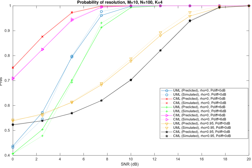
Figure 1: Simulated vs. asymptotic resolution probability of the UML and CML methods when $N=100$.

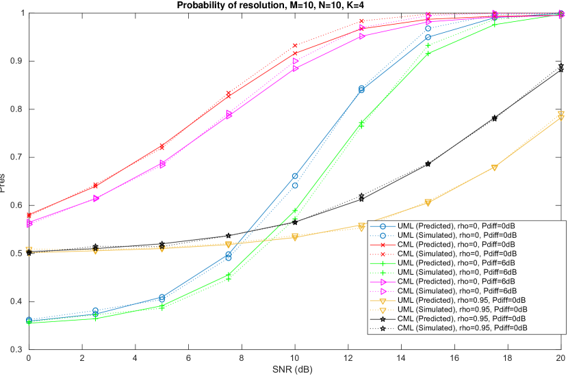
Figure 2: Simulated vs. asymptotic resolution probability of the UML and CML methods when $N=10$.

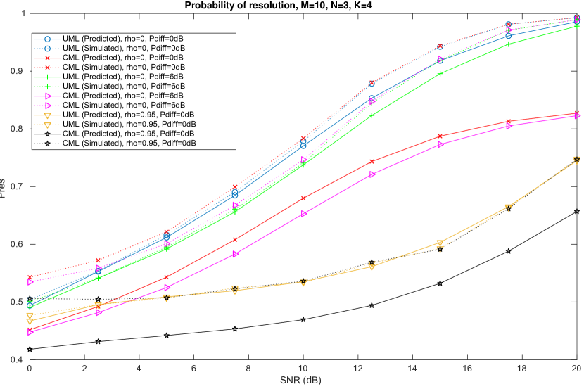
Figure 3: Simulated vs. asymptotic resolution probability of the UML and CML methods when $N=3$.

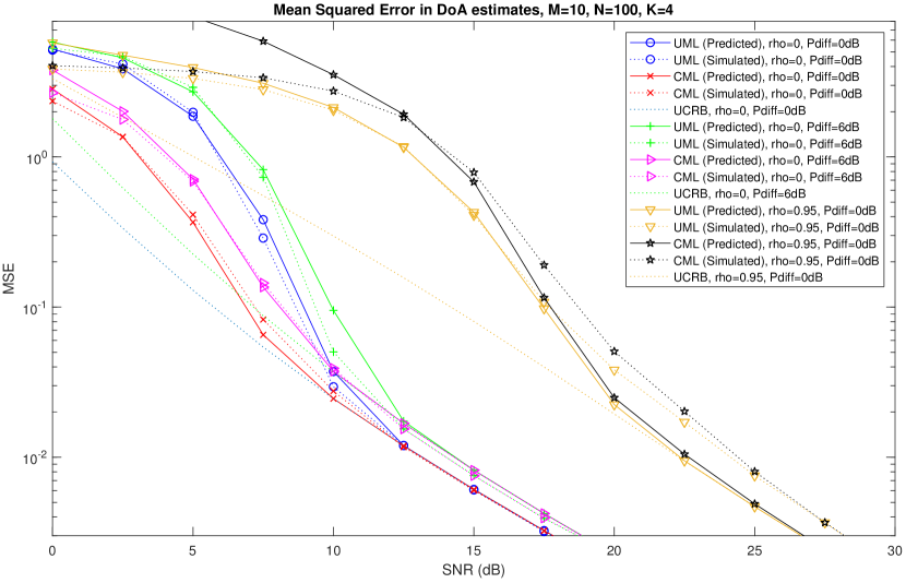
Figure 4: Simulated vs. asymptotic mean squared error (MSE) of the UML and CML methods when $N=100$.

VI Conclusions

The use of random matrix theory techniques has proven to be a very good tool to characterize the behavior of conditional and unconditional ML algorithms for DoA estimation in the threshold region. By studying the first and second order behavior of these two ML cost functions, it has been shown that the finite dimensional distributions of these two cost functions asymptotically fluctuate as multivariate Gaussian random vectors with a certain mean and covariance matrix, which have been derived in closed form. These results have been used in order to approximate and characterize the resolution probability of both methods in threshold region. These studies corroborate the fact that, in general terms, the CML method provides better resolution probabilities than UML, except for very specific cases with highly correlated source signals and relatively large sample size.

Appendix A Proof of Lemma 1

The fact that $\bar{\eta}_{C}\left(\theta\right)$ achieves its maximum at $\theta=\bar{\theta}$ is well known in the literature, as it is the case for $\bar{\eta}_{U}\left(\theta\right)$ in the oversampled regime. Thus, we will only prove the result for $\bar{\eta}_{U}\left(\theta\right)$ in the undersampled regime. Let us recall that $\mathbf{U}_{A}\left(\theta\right)=\mathbf{A}(\theta)\left(\mathbf{A}^{H}(\theta)\mathbf{A}(\theta)\right)^{-1/2}$. Observe first that we can re-write

$$\bar{\eta}_{U}\left(\theta\right)=\Upsilon\left(\mathbf{U}_{A}\left(\theta\right)\right)+\frac{M-N}{M}\log\left(\frac{1}{M-N}\operatorname*{tr}\left[\mathbf{R}\right]\right)$$

where

$$\Upsilon\left(\mathbf{U}\right)=-\frac{N}{M}+\frac{1}{M}\log\det\left[\mathbf{U}^{H}\mathbf{RU}-\xi\left(\mathbf{U}\right)\mathbf{I}_{K}\right]+\frac{M-N}{M}\log\left(1-\frac{\operatorname*{tr}\left[\mathbf{U}^{H}\mathbf{RU}\right]}{\operatorname*{tr}\left[\mathbf{R}\right]}\right)-\frac{K-N}{M}\log\left|\xi\left(\mathbf{U}\right)\right|$$

and where $\xi\left(\mathbf{U}_{A}\left(\theta\right)\right)=\phi_{0}\left(\theta\right)$, so that $\xi\left(\mathbf{U}\right)$ is the unique negative solution of the equation

$$\frac{1}{N}\operatorname*{tr}\left[\mathbf{U}^{H}\mathbf{RU}\left(\mathbf{U}^{H}\mathbf{RU}-\xi\mathbf{I}_{K}\right)^{-1}\right]=1.$$ (34)

Consider the unconstrained maximization of the function $\Upsilon\left(\mathbf{U}\right)$ with respect to the set of $M\times K$ matrices with orthogonal columns. Let $\mathbf{\Sigma}\in\mathbb{C}^{K\times K}$ be a complex Hermitian matrix that contains the Lagrange multipliers corresponding to the set of constraints $\mathbf{U}^{H}\mathbf{U=I}_{K}$. By constructing the Lagrangian associated to this optimization problem and forcing the derivatives with respect to the entries of $\mathbf{U}$ to zero we obtain the optimality conditions

$$\frac{1}{\bar{\sigma}_{N}^{2}\left(\mathbf{U}\right)}\mathbf{RU}-\mathbf{RU}\left(\mathbf{U}^{H}\mathbf{RU-}\xi\left(\mathbf{U}\right)\mathbf{I}_{K}\right)^{-1}=M\mathbf{U\Sigma}$$ (35)

where, with some abuse of notation, we have defined

$$\bar{\sigma}_{N}^{2}\left(\mathbf{U}\right)=\frac{1}{M-K}\operatorname*{tr}\left[\mathbf{R}\left(\mathbf{I}_{M}-\mathbf{UU}^{H}\right)\right].$$

Imposing the orthogonality constraint we obtain an expression for $\mathbf{\Sigma}$, which inserted into (35) leads to

$$\left[\mathbf{RU}-\mathbf{U}\left(\mathbf{U}^{H}\mathbf{RU}\right)\right]\left[\mathbf{I}_{K}-\bar{\sigma}_{N}^{2}\left(\mathbf{U}\right)\left(\mathbf{U}^{H}\mathbf{RU-}\xi\left(\mathbf{U}\right)\mathbf{I}_{K}\right)^{-1}\right]=\mathbf{0.}$$ (36)

Hence, all local minima of $\Upsilon\left(\mathbf{U}\right)$ must be zeros of one of the two factors above.

Let us first analyze the zeros of the first term, namely the solutions to $\mathbf{RU=U}(\mathbf{U}^{H}\mathbf{RU)}$. Noting that $\mathbf{U}^{H}\mathbf{RU}$ is Hermitian and positive definite, so we can consider its eigenvalue decomposition, namely $\mathbf{Q}\Lambda\mathbf{Q}^{H}$. Using this, the above equation can be rewritten as $\mathbf{RUQ=UQ}\Lambda$ and we see that the columns of matrix $\mathbf{UQ}$ are equal to $K$ different eigenvectors of $\mathbf{R}$. Since the value of the cost function is invariant to the choice of $\mathbf{Q}$, we have determined all the set of solutions corresponding to the first part of the identity in (36). Regarding the second term in (36), we need to have

$$\mathbf{U}^{H}\mathbf{RU}=\left(\xi\left(\mathbf{U}\right)+\bar{\sigma}_{N}^{2}\left(\mathbf{U}\right)\right)\mathbf{I}_{K}.$$

This means that $\mathbf{U}$ must belong to the kernel of $\mathbf{R-}\left(\xi\left(\mathbf{U}\right)+\bar{\sigma}_{N}^{2}\left(\mathbf{U}\right)\right)\mathbf{I}_{M},$ so that here again the columns of $\mathbf{U}$ must be formed by distinct eigenvectors of $\mathbf{R}$ up to right multiplication by an orthogonal matrix. Let $\lambda_{1}\leq\ldots\leq\lambda_{M}$ denote the eigenvalues of $\mathbf{R}$ (some of which may be repeated), and let $\mathcal{I}$ denote the index set of the $K$ eigenvectors of $\mathbf{R}$ in the selected matrix $\mathbf{U}$ and $\overline{\mathcal{I}}$ its complementary. At the local extrema, we see that the cost function $\Upsilon\left(\mathbf{U}\right)$ can be expressed as

$$\Upsilon\left(\mathbf{U}\right)=-\frac{N}{M}+\frac{1}{M}\log\det\mathbf{R}-\frac{M-N}{M}\log\frac{\operatorname*{tr}\left[\mathbf{R}\right]}{M-K}\\ +\frac{M-N}{M}\left(\log\left(\frac{1}{M-K}\sum_{k\in\overline{\mathcal{I}}}\lambda_{k}\right)-\frac{1}{M-K}\sum_{k\in\overline{\mathcal{I}}}\log\lambda_{k}\right)+\frac{1}{M}\frac{K-N}{M-K}\sum_{k\in\overline{\mathcal{I}}}\log\lambda_{k}\\ -\frac{1}{M}\sum_{k\in\mathcal{I}}\log\frac{\lambda_{k}}{\lambda_{k}-\xi_{\mathcal{I}}}-\frac{K-N}{M}\log\left|\xi_{\mathcal{I}}\right|$$

where $\xi_{\mathcal{I}}$ is the negative solution to

$$\frac{1}{N}\sum_{i\in\mathcal{I}}\frac{\lambda_{i}}{\lambda_{i}-\xi_{\mathcal{I}}}=1.$$

The first term is independent of $\mathcal{I}$ and can be obviated. The second term is non-negative by the arithmetic-geometric mean inequality and reaches its minimum when the eigenvalues $\left(\lambda_{k}\right)_{k\in\overline{\mathcal{I}}}$ are all equal, that is when $\overline{\mathcal{I}}=\left\{1,\ldots,M-K\right\}$ so that all these eigenvalues are equal to the noise power. Since $K>N$, the third term is minimum under the same circumstances. Regarding the final term, it can readily be seen that it decreasing in $\left(\lambda_{k}\right)_{k\in\mathcal{I}}$ because its derivative with respect to $\lambda_{j}$ is equal to

$$-\frac{1}{M}\frac{\left(-\xi_{\mathcal{I}}\right)}{\lambda_{j}\left(\lambda_{j}-\xi_{\mathcal{I}}\right)}<0$$

implying that the minimum is achieved when the selected eigenvalues are maximum, that is$\ \mathcal{I}=\left\{M-K+1,\ldots,M\right\}$.

From all the above, we conclude that $\Upsilon\left(\mathbf{U}\right)$ is minimized when the columns of $\mathbf{U}$ are selected as the eigenvectors associated with the $K$ largest eigenvalues of $\mathbf{R}$. However, these eigenvectors span the column space of $\mathbf{A}\left(\bar{\theta}\right)$ and by the manifold regularity condition one must necessarily have $\bar{\theta}=\arg\min_{\theta}\bar{\eta}_{U}\left(\theta\right)$ as we wanted to show.

Appendix B Proof of Proposition 1

In this appendix, we drop from the notation the dependence on $\ell$ (point sequence index) to simplify the exposition. Since $\ell\geq 1$, we will have $0=\gamma_{0}<\gamma_{1}<\ldots<\gamma_{\bar{M}}$. We note that we can rewrite $\mathcal{L}(\omega)$ in (23) as $\mathcal{L}(\omega)=\log\left[\omega\left(1-\Phi\left(\omega\right)\right)\right]$, where we have defined

$$\Phi\left(\omega\right)=\frac{1}{N}\sum_{m=1}^{\bar{M}}K_{m}\frac{\gamma_{m}}{\gamma_{m}-\omega}.\,$$ (37)

Let $\phi_{0}<\phi_{1}<\ldots<\phi_{\bar{M}}$ denote the $\bar{M}$ different roots of the equation $\phi\left(1-\Phi\left(\phi\right)\right)=0$. It is not difficult to see [27] that only the roots $\phi_{1},\ldots,\phi_{\bar{M}}$ are enclosed by $\mathcal{C}_{\omega}$, whereas $\phi_{0}$ is always outside the contour $\mathcal{C}_{\omega}$. Furthermore, when $K<N$ we have $\phi_{0}=0$ and $\phi_{1}>0$ whereas when $K>N$ we have $\phi_{0}<0$ and $\phi_{1}=0$. In particular, we see that $\{0\}$ is enclosed by $\mathcal{C}_{\omega}$ only in the undersampled regime ($K>N$).

First of all, note that, using the fact that $\phi_{0}\left(1-\Phi\left(\phi_{0}\right)\right)=0$ we may re-write $\mathcal{L}(\omega)$ in (23) as

$$\mathcal{L}(\omega)=\log\left[\left(\omega-\phi_{0}\right)\left(1-\widetilde{\Phi}\left(\omega\right)\right)\right]$$

where we have defined

$$\widetilde{\Phi}\left(\omega\right)=\frac{1}{N}\sum_{m=1}^{\bar{M}_{m}}\widetilde{K}_{m}\frac{\gamma_{m}}{\gamma_{m}-\omega}\quad\widetilde{K}_{m}=K_{m}\frac{\gamma_{m}}{\gamma_{m}-\phi_{0}}.$$ (38)

Consider the function $\mathcal{I}(x):[0,1]\rightarrow\mathbb{C}$, defined as

$$\mathcal{I}(x)=\frac{1}{2\pi\operatorname*{j}}{\displaystyle\oint\nolimits_{\mathcal{C}_{\omega}^{-}}}\frac{\mathcal{L}(\omega,x)}{1-\Phi\left(\omega\right)}\left(\frac{1}{M}\sum_{m=1}^{\bar{M}}\frac{K_{m}}{\gamma_{m}-\omega}\right)\frac{1}{\omega^{\prime}}d\omega$$ (39)

where $\mathcal{L}(\omega,x)=\log[(\omega-\phi_{0})(1-x\widetilde{\Phi}\left(\omega\right))]$ and where $\omega^{\prime}$ should be understood as the derivative defined in (22) as a function of $\omega$. Note that the above integral we want to solve can be expressed as $\mathcal{I}(1)$. It follows from the DCT (cf. [34, Lemma 4]) that $\mathcal{I}(x)$ is a differentiable function of $x$, and therefore we can compute $\mathcal{I}(1)$ by first computing the derivative $\mathcal{I}^{\prime}(x)$ and its primitive and then using $\mathcal{I}(0)$ to fix the value of the undetermined constant.

We consider first the integral $\mathcal{I}(0)$, which can be expressed as

$$\mathcal{I}(0)=\frac{1}{2\pi\operatorname*{j}}{\displaystyle\oint\nolimits_{\mathcal{C}_{\omega}^{-}}}\frac{\log\left(\omega-\phi_{0}\right)}{1-\Phi\left(\omega\right)}\left(\frac{1}{M}\sum_{m=1}^{\bar{M}}K_{m}\frac{1}{\gamma_{m}-\omega}\right)\frac{1}{\omega^{\prime}}d\omega.$$

Noting that $\Phi\left(0\right)\neq 1$, we see that $\phi_{k}=0$ does not constitute a singularity of the above integrand, so the poles that contribute to the above integral are $\left\{\gamma_{k},k\geq 1\right\}$ and $\left\{\phi_{k},k\geq 1,\phi_{k}\neq 0\right\}$. By simple residue calculus, we can establish that

$$\mathcal{I}(0)=\frac{1}{M}\sum_{k=1}^{\bar{M}}K_{k}\log\left(\gamma_{k}-\phi_{0}\right)-\frac{N}{M}\Phi\left(\phi_{0}\right)+\frac{N-K}{M}\log\frac{{\displaystyle\prod\nolimits_{k=1}^{\bar{M}}}\left(\gamma_{k}-\phi_{0}\right)}{{\displaystyle\prod\nolimits_{\begin{subarray}{c}k=1\\ \phi_{k}\neq 0\end{subarray}}^{\bar{M}}}\left(\phi_{k}-\phi_{0}\right)}$$

Next, we focus on the derivative $\mathcal{I}^{\prime}(x)$, which takes the form

$$\mathcal{I}^{\prime}(x)=\frac{1}{2\pi\operatorname*{j}}{\displaystyle\oint\nolimits_{\mathcal{C}_{\omega}^{+}}}\frac{\widetilde{\Phi}\left(\omega\right)\left(\frac{1}{M}\sum_{m=1}^{\bar{M}}K_{m}\frac{1}{\gamma_{m}-\omega}\right)}{\left(1-x\widetilde{\Phi}\left(\omega\right)\right)\left(1-\Phi\left(\omega\right)\right)}\frac{1}{\omega^{\prime}}d\omega.$$

Let us consider $x\in\left(0,1\right)$ and let $\widetilde{\phi}_{1}\left(x\right)<\ldots<\widetilde{\phi}_{\bar{M}}\left(x\right)$ denote the $\bar{M}$ distinct solutions to the equation $x\widetilde{\Phi}\left(\widetilde{\nu}\right)=1$. It can readily be seen following the approach in [27] that when $x\in\left(0,1\right)$ all the roots $\widetilde{\phi}_{1}\left(x\right),\ldots,\widetilde{\phi}_{\bar{M}}\left(x\right)$ are located inside $\mathcal{C}_{\omega}$. Observing that $\omega=0$ is not a singularity of the above integrand, we see that the poles inside the contour are $\{\gamma_{k},k\geq 1\}$, $\{\phi_{k},k\geq 1,\phi_{k}\neq 0\}$ and $\{\widetilde{\phi}_{k}\left(x\right),k\geq 1\}$. Computing the corresponding residues, we find that

$$\mathcal{I}^{\prime}(x)=\frac{1}{x}\left(\frac{K}{M}+\frac{N-K}{M}\bar{M}\right)+\frac{1}{x^{2}}\frac{N}{M}\sum_{k=1}^{\bar{M}}\frac{K_{k}}{\widetilde{K}_{k}}\\ +\frac{1}{M}\sum_{\begin{subarray}{c}k=1\\ \widetilde{\phi}_{k}\left(x\right)\neq 0\end{subarray}}^{\bar{M}}\sum_{m=1}^{\bar{M}}K_{m}\left(1+\frac{\gamma_{m}}{\gamma_{m}-\widetilde{\phi}_{k}\left(x\right)}\right)\frac{\widetilde{\phi}_{k}^{\prime}\left(x\right)}{\gamma_{m}-\widetilde{\phi}_{k}\left(x\right)}\\ +\frac{N-K}{M}\left(\sum_{\begin{subarray}{c}k=1\\ \phi_{k}\neq 0\end{subarray}}^{\bar{M}}\frac{\widetilde{\Phi}\left(\phi_{k}\right)}{1-x\widetilde{\Phi}\left(\phi_{k}\right)}-\sum_{\begin{subarray}{c}k=1\\ \widetilde{\phi}_{k}\left(x\right)\neq 0\end{subarray}}^{\bar{M}}\frac{\Phi^{\prime}\left(\widetilde{\phi}_{k}\left(x\right)\right)\widetilde{\phi}_{k}^{\prime}\left(x\right)}{1-\Phi\left(\widetilde{\phi}_{k}\left(x\right)\right)}\right)$$

where we have used the fact that, for $k>1$, we have $x\widetilde{\Phi}(\widetilde{\phi}_{k}(x))=\Phi(\phi_{k})=1$ and that $\widetilde{\phi}_{k}\left(x\right)$ is a differentiable function of $x$ with derivative

$$\widetilde{\phi}_{k}^{\prime}\left(x\right)=\left(\frac{-x^{2}}{N}\sum_{m=1}^{\bar{M}}\widetilde{K}_{m}\frac{\gamma_{m}}{\left(\gamma_{m}-\widetilde{\phi}_{k}\left(x\right)\right)^{2}}\right)^{-1}.$$

One can easily find a primitive of $\mathcal{I}^{\prime}(x)$ and fix the undetermined constraint according to the value of $\mathcal{I}(0)$. In this process, one needs to use the fact that, for $k\geq 1$, when $x\rightarrow 0$ we have $\widetilde{\phi}_{k}\left(x\right)\rightarrow\gamma_{k}$, $x^{-1}(\gamma_{k}-\widetilde{\phi}_{k}\left(x\right))\rightarrow\frac{\gamma_{k}}{N}\widetilde{K}_{k}$ and

$$\frac{1}{x}\left(\frac{\gamma_{k}-\widetilde{\phi}_{k}\left(x\right)}{x}-\frac{\gamma_{k}}{N}\widetilde{K}_{k}\right)\rightarrow\frac{\gamma_{k}}{N}\widetilde{K}_{k}\frac{1}{N}\sum_{\begin{subarray}{c}m=1\\ m\neq k\end{subarray}}^{\bar{M}}\widetilde{K}_{m}\frac{\gamma_{m}}{\gamma_{m}-\gamma_{k}}.$$

Once we have fixed the undetermined constant, we can obtain

$$\mathcal{I}(x) =\frac{1}{M}\sum_{k=1}^{\bar{M}}K_{k}\log\left(\gamma_{k}-\phi_{0}\right)-\frac{N}{M}\Phi\left(\phi_{0}\right)$$

$$+\frac{N-K}{M}\log\left|\left(1-x\widetilde{\Phi}\left(\phi_{0}\right)1_{\phi_{0}\neq 0}\right)\frac{{\displaystyle\prod\nolimits_{k=1}^{\bar{M}}}\left(\gamma_{k}-\phi_{0}\right)}{{\displaystyle\prod\nolimits_{\begin{subarray}{c}k=1\\ \phi_{k}\neq 0\end{subarray}}^{\bar{M}}}\left(\phi_{k}-\phi_{0}\right)}\right|$$

$$+\xi_{1}(x)+\xi_{2}(x)+\xi_{3}(x)$$

where $1_{\left\{\text{\textperiodcentered}\right\}}$ is the indicator function and where we have defined

$$\xi_{1}(x) =\frac{N-K}{M}\log\left|\frac{\prod\nolimits_{k=1}^{\bar{M}}\left(1-\Phi\left(\widetilde{\phi}_{k}\left(x\right)\right)\right)}{\prod\nolimits_{\begin{subarray}{c}k=0\\ \phi_{k}\neq 0\end{subarray}}^{\bar{M}}\left(1-x\widetilde{\Phi}\left(\phi_{k}\right)\right)}\prod\limits_{k=1}^{\bar{M}}\left(\frac{\widetilde{K}_{k}}{K_{k}}x\right)\right|$$

$$\xi_{2}(x) =\frac{1}{M}\sum_{m=1}^{\bar{M}}K_{m}\log\left|\frac{x\frac{\gamma_{m}}{N}\widetilde{K}_{m}\prod\nolimits_{\begin{subarray}{c}k=1\\ k\neq m\end{subarray}}^{\bar{M}}\left(\gamma_{m}-\gamma_{k}\right)}{\prod\nolimits_{k=1}^{\bar{M}}\left(\gamma_{m}-\widetilde{\phi}_{k}\left(x\right)\right)}\right|$$

$$\xi_{3}(x) =\frac{1}{M}\sum_{m=1}^{\bar{M}}\sum_{k=1}^{\bar{M}}\frac{K_{m}\gamma_{m}}{\gamma_{m}-\widetilde{\phi}_{k}\left(x\right)}+\frac{1}{M}\sum_{k=1}^{\bar{M}}\sum_{\begin{subarray}{c}m=1\\ m\neq k\end{subarray}}^{\bar{M}}\frac{K_{k}}{\widetilde{K}_{k}}\frac{\widetilde{K}_{m}\gamma_{m}}{\gamma_{m}-\gamma_{k}}$$

$$+\frac{1}{M}\sum_{k=1}^{\bar{M}}\sum_{\begin{subarray}{c}m=1\\ m\neq k\end{subarray}}^{\bar{M}}\frac{K_{m}\gamma_{m}}{\gamma_{k}-\gamma_{m}}-\frac{1}{x}\frac{N}{M}\sum_{k=1}^{\bar{M}}\frac{K_{k}}{\widetilde{K}_{k}}.$$

Lemma 2

For any $x\in\left(0,1\right)$, it holds that

$$\xi_{1}(x)=\xi_{2}(x)=\xi_{3}(x)=0.$$

Furthermore,

$$\frac{\prod\nolimits_{\begin{subarray}{c}k=1\\ \phi_{k}\neq 0\end{subarray}}^{\bar{M}}\left(\phi_{k}-\phi_{0}\right)}{\prod\nolimits_{k=1}^{\bar{M}}\left(\gamma_{k}-\phi_{0}\right)}=\left\{\begin{array}[c]{ccc}\frac{1}{N}\sum_{m=1}^{\bar{M}}K_{m}\frac{\gamma_{m}}{\left(\gamma_{m}-\phi_{0}\right)^{2}}&&\phi_{0}\neq 0\\ \frac{N-K}{N}&&\phi_{0}=0.\end{array}\right.$$ (40)

Proof:

See Appendix E.∎

From all the above, we see that when $K<N$ the function $\mathcal{I}(x)$ is constant in $x$ and equal to the value in statement of the proposition. Finally when $K>N$ we will have

$$\mathcal{I}(x) =\frac{1}{M}\sum_{k=1}^{\bar{M}}K_{k}\log\left(\gamma_{k}-\phi_{0}\right)-\frac{N}{M}+\frac{N-K}{M}\log\left|\phi_{0}\right|$$

$$+\frac{N-K}{M}\log\left|\frac{1-x\widetilde{\Phi}\left(\phi_{0}\right)}{1-\widetilde{\Phi}\left(\phi_{0}\right)}\right|$$

and therefore $\mathcal{I}(1)$ is equal to the value in the statement of the proposition.

Appendix C Solution to the covariance integrals $\Gamma_{1}^{(\ell,m)},\Gamma_{2}^{(\ell,m)}$

In this appendix, we provide an alternative solution to the covariance integrals in (30)-(31). We will consider the case $\ell\geq 1,m\geq 1$, since the cases $\ell=0$ and/or $m=0$ can be obtained by a simple renumbering of the eigenvalues. Both integrals are particular instances of the generic covariance integral given in (28), where we recall that we can express

$$\Phi_{\ell,m}\left(\omega_{1},\omega_{2}\right)=-\frac{\partial^{2}\log\left(1-\Psi_{\ell,m}\left(\omega_{1},\omega_{2}\right)\right)}{\partial\omega_{1}\partial\omega_{2}}$$

where the partial derivatives are well defined because at the contours we have $\left|\Psi_{\ell,m}\left(\omega_{1},\omega_{2}\right)\right|<1$ (simply use Cauchy-Schwarz and apply the results in [27, Appendix I]). Therefore, using the integration by parts formula we can alternatively express (28) as

$$\left\{\Gamma\right\}_{\ell,m}=-\frac{1}{2\pi\operatorname*{i}}\frac{1}{2\pi\operatorname*{i}}\oint\nolimits_{\mathcal{C}_{\omega_{\ell}}^{+}}\oint\nolimits_{\mathcal{C}_{\omega_{m}}^{+}}\frac{dg_{\ell}\left(\omega_{1}\right)}{d\omega_{1}}\frac{dg_{m}\left(\omega_{2}\right)}{d\omega_{2}}\log\left(1-\Psi_{\ell,m}\left(\omega_{1},\omega_{2}\right)\right)d\omega_{1}d\omega_{2}.$$

This means that we can re-write $\Gamma_{1}^{(\ell,m)}$ and $\Gamma_{2}^{(\ell,m)}$ as

$$\Gamma_{1}^{(\ell,m)} =-\frac{1}{2\pi\operatorname*{i}}\oint\nolimits_{\mathcal{C}_{\omega_{\ell}}^{+}}\frac{dz_{1}}{d\omega_{1}}I(\omega_{1})d\omega_{1}$$

$$\Gamma_{2}^{(\ell,m)} =-\frac{1}{2\pi\operatorname*{i}}\oint\nolimits_{\mathcal{C}_{\omega_{\ell}}^{+}}\frac{d\mathcal{L}_{\ell}(\omega_{1})}{d\omega_{1}}I(\omega_{1})d\omega_{1}$$

where $\mathcal{L}_{m}(\omega)$ is defined in (23) and where we have defined the integral

$$I(\omega_{1})=\frac{1}{2\pi\operatorname*{i}}\oint\nolimits_{\mathcal{C}_{\omega_{m}}^{+}}\frac{d\mathcal{L}_{m}(\omega_{2})}{d\omega_{2}}\log\left(1-\Psi_{\ell,m}\left(\omega_{1},\omega_{2}\right)\right)d\omega_{2}.$$

In order to solve this integral, we consider the singular value decomposition

$$\mathbf{R}_{\ell}^{1/2}=\mathbf{P}_{A}^{(\ell)}\mathbf{R}^{1/2}=\sum_{r=0}^{\bar{M}_{\ell}}\sqrt{\gamma_{r}^{(\ell)}}\mathbf{U}_{r}^{(\ell)}\left(\mathbf{V}_{r}^{(\ell)}\right)^{H}$$

where $\bar{M}_{\ell}+1$ is the total number of singular values of $\mathbf{R}_{\ell}^{1/2}$ (including $\{0\}$ when $\ell>0$). With all these definitions, we may express the function $\Psi_{\ell,m}$ as

$$\Psi_{\ell,m}\left(\omega_{1},\omega_{2}\right)=\sum_{r=0}^{\bar{M}_{\ell}}\sum_{k=0}^{\bar{M}_{m}}\kappa_{rk}^{\ell m}\frac{\gamma_{r}^{(\ell)}\gamma_{k}^{(m)}}{\left(\gamma_{r}^{(\ell)}-\omega_{1}\right)\left(\gamma_{k}^{(m)}-\omega_{2}\right)}$$

$$\kappa_{rk}^{\ell m}=\frac{1}{N}\operatorname*{tr}\left[\mathbf{V}_{r}^{(\ell)}\left(\mathbf{V}_{r}^{(\ell)}\right)^{H}\mathbf{V}_{k}^{(m)}\left(\mathbf{V}_{k}^{(m)}\right)^{H}\right].$$

and note that this notation is valid for $\ell,m\geq 0$. Using the definition of $\phi_{0}^{(m)}$, we can find an equivalent definition of the function $\mathcal{L}_{m}(\omega_{2})$ that will be more convenient from now on, that is

$$\mathcal{L}_{m}(\omega_{2})=\log\left[\left(\omega_{2}-\phi_{0}^{(m)}\right)\left(1-\frac{1}{N}\sum_{k=1}^{\bar{M}_{m}}\widetilde{K}_{k}^{(m)}\frac{\gamma_{k}^{(m)}}{\gamma_{k}^{(m)}-\omega_{2}}\right)\right]$$ (41)

where

$$\widetilde{K}_{k}^{(m)}=K_{k}^{(m)}\frac{\gamma_{k}^{(m)}}{\gamma_{k}^{(m)}-\phi_{0}^{(m)}}.$$

In order to be able to handle both the undersampled and oversampled cases, we let $0\leq\widetilde{\phi}_{1}^{(m)}<\ldots<\widetilde{\phi}_{\bar{M}_{m}}^{(m)}$ denote the $\bar{M}_{m}$ roots of the equation $\widetilde{\Phi}^{(m)}(\widetilde{\phi})=1$, where $\widetilde{\Phi}^{(m)}\left(\phi\right)$ is defined as in (38) but replacing all quantities associated with $\mathbf{R}$ by the equivalent ones associated with $\mathbf{R}_{m}$.

C-A Computation of $I(\omega_{1})$

In order to find a close form expression for $I(\omega_{1})$, we will follow the same approach as in the proof of Proposition 1 above. More specifically, we express $I(\omega_{1})=I(\omega_{1},1)$ where $I(\omega_{1},x)$ is a differentiable function of $x\in\left[0,1\right]$ defined as

$$I(\omega_{1},x)=\frac{1}{2\pi\operatorname*{i}}\oint\nolimits_{\mathcal{C}_{\omega_{m}}^{+}}\frac{d\mathcal{L}_{m}(\omega_{2})}{d\omega_{2}}\log\left(1-x\Psi_{\ell,m}\right)d\omega_{2}.$$

Obviously, we will have $I(\omega_{1},0)=0$. On the other hand, using the DCT one can see that $I(\omega_{1},x)$ is a differentiable function of $x\in[0,1]$ with derivative

$$\frac{\partial I(\omega_{1},x)}{\partial x}=\frac{-1}{2\pi\operatorname*{i}}\oint\nolimits_{\mathcal{C}_{\omega_{m}}^{+}}\frac{d\mathcal{L}_{m}(\omega_{2})}{d\omega_{2}}\frac{\Psi_{\ell,m}}{1-x\Psi_{\ell,m}}d\omega_{2}.$$

One can trivially find a closed form expression for the above integral using conventional residue calculus. One only needs to realize that, since $\phi_{0}^{(m)}$ is never enclosed by $\mathcal{C}_{\omega_{m}}$ (the proof is similar to that of Lemma 3 below), the above integrand only has singularities at the points $\{\gamma_{k}^{(m)},\widetilde{\phi}_{k}^{(m)},k=1,\ldots,\bar{M}_{m}\}$ plus the solutions to the equation $x\Psi_{\ell,m}\left(\omega_{1},\omega_{2}\right)=1$ as a function of $\omega_{1}$. The following lemma establishes that there exist exactly $\bar{M}_{m}$ solutions to this equation enclosed by $\mathcal{C}_{\omega_{m}}$, which will be denoted as $\zeta_{j}^{(\ell,m)}\left(\omega_{1},x\right)$, $j=1,\ldots,\bar{M}_{m}$.

Lemma 3

Define, for $\ell\geq 0$, the region

$$\Omega_{\ell}=\left\{\omega\in\mathbb{C}:\frac{1}{N}\sum_{r=0}^{\bar{M}_{\ell}}K_{r}^{(\ell)}\left|\frac{\gamma_{r}^{(\ell)}}{\gamma_{r}^{(\ell)}-\omega}\right|^{2}<1\right\}$$

and let $\omega_{1}\in\Omega_{\ell}$. Then, when $m\geq 1$ and for $x\in(0,1]$, the following equation in the complex variable $\zeta$

$$x\Psi_{\ell,m}\left(\omega_{1},\zeta\right)=1.$$ (42)

has exactly $\bar{M}_{m}$ roots inside $\partial\Omega_{m}$.

Proof:

See Appendix F.∎

It can easily be seen that $\{\widetilde{\phi}_{k}^{(m)},k=1,\ldots,\bar{M}_{m}\}$ are always enclosed by the contour $\partial\Omega_{m}$. Since the contour $\mathcal{C}_{\omega_{m}}^{+}$ is always enclosing the region $\Omega_{m}$ (cf. [27]) we can readily compute the value of $\partial I(\omega_{1},x)/\partial x$ using conventional Cauchy calculus,

$$\frac{\partial I(\omega_{1},x)}{\partial x}=-\frac{\bar{M}_{m}}{x}-\sum_{j=1}^{\bar{M}_{m}}\frac{\Psi_{\ell,m}\left(\omega_{1},\widetilde{\phi}_{j}^{(m)}\right)}{1-x\Psi_{\ell,m}\left(\omega_{1},\widetilde{\phi}_{j}^{(m)}\right)}+\\ +\sum_{j=1}^{\bar{M}_{m}}\left(\frac{\widetilde{\Phi}^{(m)\prime}\left(\zeta_{j}^{(\ell,m)}\left(\omega_{1,}x\right)\right)}{1-\widetilde{\Phi}^{(m)}\left(\zeta_{j}^{(\ell,m)}\left(\omega_{1,}x\right)\right)}-\frac{1}{\zeta_{j}^{(\ell,m)}\left(\omega_{1},x\right)-\phi_{0}^{(m)}}\right)\frac{\partial\zeta_{j}^{(\ell,m)}\left(\omega_{1},x\right)}{\partial x}$$

where $\widetilde{\Phi}^{(m)\prime}$ denotes the derivative of $\widetilde{\Phi}^{(m)}$ and where we have used the fact that $\zeta_{j}^{(\ell,m)}\left(\omega_{1},x\right)$ is a differentiable function of $x$ with derivative

$$\frac{\partial\zeta_{j}^{(\ell,m)}\left(\omega_{1},x\right)}{\partial x}=\left(-x^{2}\left.\frac{\partial\Psi_{\ell,m}\left(\omega_{1},\omega_{2}\right)}{\partial\omega_{2}}\right|_{\omega_{2}=\zeta_{j}^{(\ell,m)}\left(\omega_{1},x\right)}\right)^{-1}.$$

We can therefore find a primitive of $\partial I(\omega_{1},x)/\partial x$ and force the value of $I(\omega_{1},0)=0$ to fix the undetermined constraint. In order to do this, we need to use the fact that $\lim_{x\rightarrow 0}\zeta_{j}^{(\ell,m)}\left(\omega_{1,}x\right)=\gamma_{j}^{(m)}$ and

$$\lim_{x\rightarrow 0}x^{-1}\left(\gamma_{j}^{(m)}-\zeta_{j}^{(\ell,m)}\left(\omega_{1,}x\right)\right)=\sum_{r=1}^{\bar{M}_{\ell}}\kappa_{rj}^{\ell m}\frac{\gamma_{r}^{(\ell)}\gamma_{j}^{(m)}}{\gamma_{r}^{(\ell)}-\omega_{1}}.$$

All this leads to

$$I(\omega_{1},x)=-\log\left(1-x\Psi_{\ell,m}\left(\omega_{1},\phi_{0}^{(m)}\right)\right)+\xi_{1}(\omega_{1},x)+\xi_{2}(\omega_{1},x)$$

where we have defined

$$\xi_{1}(\omega_{1},x)=\sum_{j=1}^{\bar{M}_{m}}\log\left(\frac{1-x\Psi_{\ell,m}\left(\omega_{1},\widetilde{\phi}_{j}^{(m)}\right)}{1-\widetilde{\Phi}^{(m)}\left(\zeta_{j}^{(\ell,m)}\left(\omega_{1},x\right)\right)}\right) -\sum_{j=1}^{\bar{M}_{m}}\log\left(\frac{xN}{\widetilde{K}_{j}^{(m)}}\sum_{r=1}^{\bar{M}_{\ell}}\kappa_{rj}^{\ell m}\frac{\gamma_{r}^{(\ell)}}{\omega_{1}-\gamma_{r}^{(\ell)}}\right)$$

$$\xi_{2}(\omega_{1},x)=\log\left(1-x\Psi_{\ell,m}\left(\omega_{1},\phi_{0}^{(m)}\right)\right) +\sum_{j=1}^{\bar{M}_{m}}\log\left(\frac{\gamma_{i}^{(m)}-\phi_{0}^{(m)}}{\zeta_{i}^{(\ell,m)}\left(\omega_{1},x\right)-\phi_{0}^{(m)}}\right)$$

Lemma 4

For any $x\in\left(0,1\right]$, we have $\xi_{1}(\omega_{1},x)=\xi_{2}(\omega_{1},x)=0$.

Proof:

See Appendix G.∎

By simply taking  $x=1$ in the resulting expression for $I(\omega_{1},x)$ we get $I(\omega_{1})=-\log(1-\Psi_{\ell,m}(\omega_{1},\phi_{0}^{(m)}))$.

C-B Computation of $\Gamma_{1}^{(\ell,m)}$

By applying the integration by parts formula we can write

$$\Gamma_{1}^{(\ell,m)}=\frac{1}{2\pi\operatorname*{i}}\oint\nolimits_{\mathcal{C}_{\omega_{\ell}}^{+}}z_{1}\frac{\sum_{r=1}^{\bar{M}_{\ell}}\widetilde{\kappa}_{r}^{\ell m}\frac{\gamma_{r}^{(\ell)}}{\left(\gamma_{r}^{(\ell)}-\omega_{1}\right)^{2}}}{1-\sum_{r=1}^{\bar{M}_{\ell}}\widetilde{\kappa}_{r}^{\ell m}\frac{\gamma_{r}^{(\ell)}}{\gamma_{r}^{(\ell)}-\omega_{1}}}d\omega_{1}$$

where we have defined

$$\widetilde{\kappa}_{r}^{\ell m}=\sum_{k=1}^{\bar{M}_{m}}\kappa_{rk}^{\ell m}\frac{\gamma_{k}^{(m)}}{\gamma_{k}^{(m)}-\phi_{0}^{(m)}}.$$

Let $\nu_{j}^{(\ell,m)}$ denote the solutions to the equation

$$1=\sum_{r=0}^{\bar{M}_{\ell}}\widetilde{\kappa}_{r}^{\ell m}\frac{\gamma_{r}^{(\ell)}}{\gamma_{r}^{(\ell)}-\nu_{j}^{(\ell,m)}}.$$ (43)

Lemma 5

This equation has $\bar{M}_{\ell}$ distinct solutions, namely  $\nu_{1}^{(\ell,m)}<\ldots<\nu_{\bar{M}_{\ell}}^{(\ell,m)}$, all of which are located inside $\mathcal{C}_{\omega_{\ell}}^{+}$.

Proof:

See Appendix H.∎

Hence, we can obtain the value of $\Gamma_{1}^{(\ell,m)}$ by using classical residue calculus on the poles $\{\gamma_{j}^{(\ell)},\nu_{j}^{(\ell,m)}\}$ that are enclosed by $\mathcal{C}_{\omega_{\ell}}^{+}$. Close examination of the integrand of $\Gamma_{1}^{(\ell,m)}$ leads to the conclusion that the only poles enclosed by $\mathcal{C}_{\omega_{\ell}}^{+}$ are $\{\gamma_{j}^{(\ell)},\nu_{j}^{(\ell,m)},j=1,\ldots,\bar{M}_{\ell}\}$, and direct computation of the residues allows us to conclude that

$$\Gamma_{1}^{(\ell,m)}=\sum_{j=1}^{\bar{M}_{\ell}}K_{j}^{(\ell)}\gamma_{j}^{(\ell)}+\sum_{j=1}^{\bar{M}_{\ell}}\gamma_{j}^{(\ell)}\left(1-\sum_{\begin{subarray}{c}r=1\\ r\neq j\end{subarray}}^{\bar{M}_{\ell}}K_{r}^{(\ell)}\frac{\gamma_{r}^{(\ell)}}{\gamma_{r}^{(\ell)}-\gamma_{j}^{(\ell)}}\right)+\\ -\sum_{j=1}^{\bar{M}_{\ell}}\nu_{j}^{(\ell,m)}\left(1-\sum_{r=1}^{\bar{M}_{\ell}}K_{r}^{(\ell)}\frac{\gamma_{r}^{(\ell)}}{\gamma_{r}^{(\ell)}-\nu_{j}^{(\ell,m)}}\right)-\sum_{j=1}^{\bar{M}_{\ell}}\frac{K_{j}^{(\ell)}}{\widetilde{\kappa}_{j}^{\ell m}}\gamma_{j}^{(\ell)}\left(1-\sum_{\begin{subarray}{c}r=1\\ r\neq j\end{subarray}}^{\bar{M}_{\ell}}\widetilde{\kappa}_{r}^{\ell m}\frac{\gamma_{r}^{(\ell)}}{\gamma_{r}^{(\ell)}-\gamma_{j}^{(\ell)}}\right)$$

In order to simplify this, we introduce the following lemma.

Lemma 6

Let $\ell\geq 1$. For $j=1,\ldots,\bar{M}_{\ell}$ we have

$$\sum_{r=1}^{\bar{M}_{\ell}}\nu_{r}^{(\ell,m)} =\sum_{r=1}^{\bar{M}_{\ell}}\gamma_{r}^{(\ell)}-\sum_{r=1}^{\bar{M}_{\ell}}\widetilde{\kappa}_{r}^{\ell m}\gamma_{r}^{(\ell)}$$ (44)

$$\sum_{i=1}^{\bar{M}_{\ell}}\frac{\widetilde{\kappa}_{j}^{\ell m}\gamma_{j}^{(\ell)}}{\nu_{i}^{(\ell,m)}-\gamma_{j}^{(\ell)}} =\sum_{\begin{subarray}{c}r=1\\ r\neq j\end{subarray}}^{\bar{M}_{\ell}}\widetilde{\kappa}_{r}^{\ell m}\frac{\gamma_{r}^{(\ell)}}{\gamma_{r}^{(\ell)}-\gamma_{j}^{(\ell)}}+\sum_{\begin{subarray}{c}i=1\\ i\neq j\end{subarray}}^{\bar{M}_{\ell}}\widetilde{\kappa}_{j}^{\ell m}\frac{\gamma_{j}^{(\ell)}}{\gamma_{i}^{(\ell)}-\gamma_{j}^{(\ell)}}-1$$ (45)

Proof:

See Appendix I.∎

Now, using (44)-(45) in the expression of $\Gamma_{1}^{(\ell,m)}$ we directly obtain

$$\Gamma_{1}^{(\ell,m)}=\sum_{r=1}^{\bar{M}_{\ell}}\widetilde{\kappa}_{r}^{\ell m}\gamma_{r}^{(\ell)}=\frac{1}{N}\operatorname*{tr}\left[\mathbf{R}^{1/2}\mathbf{P}_{A}^{(\ell)}\mathbf{R}^{1/2}\sum_{k=1}^{\bar{M}_{m}}\frac{\gamma_{k}^{(m)}}{\gamma_{k}^{(m)}-\phi_{0}^{(m)}}\mathbf{V}_{k}^{(m)}\left(\mathbf{V}_{k}^{(m)}\right)^{H}\right]$$

which can alternatively be expressed as in (32).

C-C Computation of $\Gamma_{2}^{(\ell,m)}$

Using the expression of $I(\omega_{1})$ and the analycity of $\mathcal{L}_{\ell}(\omega_{1})$, we may express $\Gamma_{2}^{(\ell,m)}$ as $\Gamma_{2}^{(\ell,m)}(1)$ where

$$\Gamma_{2}^{(\ell,m)}\left(x\right)=\frac{-1}{2\pi\operatorname*{i}}\oint\nolimits_{\mathcal{C}_{\omega_{\ell}}^{+}}\frac{d\mathcal{L}_{\ell}(\omega_{1})}{d\omega_{1}}\log\left(1-x\Psi_{\ell,m}\left(\omega_{1},\phi_{0}^{(m)}\right)\right)d\omega_{1}$$

is a differentiable function of $x$ in the unit interval. Taking the definition of $\mathcal{L}_{\ell}(\omega_{1})$ in (41), we can readily see that $\Gamma_{2}^{(\ell,m)}\left(0\right)=0$. On the other hand, using the dominated convergence theorem we can compute the derivative as

$$\frac{d\Gamma_{2}^{(\ell,m)}\left(x\right)}{dx}=\frac{1}{2\pi\operatorname*{i}}\oint\nolimits_{\mathcal{C}_{\omega_{\ell}}^{+}}\frac{d\mathcal{L}_{\ell}(\omega_{1})}{d\omega_{1}}\frac{\Psi_{\ell,m}\left(\omega_{1},\phi_{0}^{(m)}\right)}{1-x\Psi_{\ell,m}\left(\omega_{1},\phi_{0}^{(m)}\right)}d\omega_{1}.$$

This integral can be computed via conventional Cauchy integration, using the fact that the singularities are located at the points $\{\gamma_{r}^{(\ell)},\widetilde{\phi}_{j}^{(\ell)},\nu_{j}^{(\ell,m)}\left(x\right),j=1,\ldots,\bar{M}_{\ell}\}$ where we recall that $\widetilde{\phi}_{j}^{(\ell)}$ are the solutions to $\widetilde{\Phi}^{(\ell)}\left(\omega_{1}\right)=1$ and where we have introduced the quantities $\nu_{j}^{(\ell,m)}\left(x\right)$, defined as the solutions to the equation $x\Psi_{\ell,m}(\omega_{1},\phi_{0}^{(m)})=1$. It can be shown that all these points are inside $\mathcal{C}_{\omega_{\ell}}$. Computing the corresponding residues, we obtain

$$\frac{d\Gamma_{2}^{(\ell,m)}\left(x\right)}{dx}=\frac{1}{x}\bar{M}_{\ell}+\sum_{j=1}^{\bar{M}_{\ell}}\frac{\sum_{r=1}^{\bar{M}_{\ell}}\widetilde{\kappa}_{r}^{\ell m}\frac{\gamma_{r}^{(\ell)}}{\gamma_{r}^{(\ell)}-\widetilde{\phi}_{j}^{(\ell)}}}{1-x\sum_{r=1}^{\bar{M}_{\ell}}\widetilde{\kappa}_{r}^{\ell m}\frac{\gamma_{r}^{(\ell)}}{\gamma_{r}^{(\ell)}-\widetilde{\phi}_{j}^{(\ell)}}}+\sum_{j=1}^{\bar{M}_{\ell}}\left(\frac{1}{\nu_{j}^{(\ell,m)}\left(x\right)-\phi_{0}^{(\ell)}}-\frac{\Phi^{(\ell)\prime}(\nu_{j}^{(\ell,m)}\left(x\right))}{1-\Phi^{(\ell)}(\nu_{j}^{(\ell,m)}\left(x\right))}\right)\frac{d\nu_{j}^{(\ell,m)}\left(x\right)}{dx}$$

where $\Phi^{(\ell)}(\omega_{1})$ is defined as in (38) and where $\Phi^{(\ell)\prime}(\omega_{1})$ denotes its derivative. We can readily find a primitive of the above equation and finally obtain

$$\Gamma_{2}^{(\ell,m)}=-\sum_{j=1}^{\bar{M}_{\ell}}\log\left|1-\sum_{r=1}^{\bar{M}_{\ell}}\widetilde{\kappa}_{r}^{\ell m}\frac{\gamma_{r}^{(\ell)}}{\gamma_{r}^{(\ell)}-\widetilde{\phi}_{j}^{(\ell)}}\right|\\ +\sum_{j=1}^{\bar{M}_{\ell}}\log\left|N\frac{\widetilde{\kappa}_{j}^{\ell m}}{\widetilde{K}_{j}^{(\ell)}}\frac{\nu_{j}^{(\ell,m)}-\phi_{0}^{(\ell)}}{\gamma_{j}^{(\ell)}-\phi_{0}^{(\ell)}}\right|+\sum_{j=1}^{\bar{M}_{\ell}}\log\left|1-\frac{1}{N}\sum_{r=1}^{\bar{M}_{\ell}}\widetilde{K}_{r}^{(\ell)}\frac{\gamma_{r}^{(\ell)}}{\gamma_{r}^{(\ell)}-\nu_{j}^{(\ell,m)}}\right|$$

where we have used the fact that $\Gamma_{2}^{(\ell,m)}(0)=0$ to fix the indeterminate constraint. We can now simplify this expression using the following result.

Lemma 7

The following identities hold for any $j\geq 1$,

$$\prod\limits_{r=1}^{\bar{M}_{\ell}}\frac{\nu_{r}^{(\ell,m)}-\widetilde{\phi}_{j}^{(\ell)}}{\gamma_{r}^{(\ell)}-\widetilde{\phi}_{j}^{(\ell)}} =1-\sum_{r=1}^{\bar{M}_{\ell}}\widetilde{\kappa}_{r}^{\ell m}\frac{\gamma_{r}^{(\ell)}}{\gamma_{r}^{(\ell)}-\widetilde{\phi}_{j}^{(\ell)}}$$

$$\prod\limits_{r=1}^{\bar{M}_{\ell}}\left(\nu_{r}^{(\ell,m)}-\gamma_{j}^{(\ell)}\right) =-\widetilde{\kappa}_{j}^{\ell m}\gamma_{j}^{(\ell)}\prod\limits_{\begin{subarray}{c}k=1\\ k\neq j\end{subarray}}^{\bar{M}_{\ell}}\left(\gamma_{k}^{(\ell)}-\gamma_{j}^{(\ell)}\right)$$

$${\displaystyle\prod\limits_{k=1}^{\bar{M}_{\ell}}}\frac{\widetilde{\phi}_{k}^{(\ell)}-\nu_{j}^{(\ell,m)}}{\gamma_{k}^{(\ell)}-\nu_{j}^{(\ell,m)}} =1-\frac{1}{N}\sum_{r=1}^{\bar{M}_{\ell}}\widetilde{K}_{r}^{(\ell)}\frac{\gamma_{r}^{(\ell)}}{\gamma_{r}^{(\ell)}-\nu_{j}^{(\ell,m)}}$$

$${\displaystyle\prod\limits_{k=1}^{\bar{M}_{\ell}}}\left(\widetilde{\phi}_{k}^{(\ell)}-\gamma_{j}^{(\ell)}\right) =-\frac{1}{N}\widetilde{K}_{j}^{(\ell)}\gamma_{j}^{(\ell)}{\displaystyle\prod\limits_{\begin{subarray}{c}k=1\\ k\neq j\end{subarray}}^{\bar{M}_{\ell}}}\left(\gamma_{k}^{(\ell)}-\gamma_{j}^{(\ell)}\right)$$

$$\prod\limits_{r=1}^{\bar{M}_{\ell}}\frac{\nu_{r}^{(\ell,m)}-\phi_{0}^{(\ell)}}{\gamma_{k}^{(\ell)}-\phi_{0}^{(\ell)}} =1-\sum_{r=1}^{\bar{M}_{\ell}}\widetilde{\kappa}_{r}^{\ell m}\frac{\gamma_{r}^{(\ell)}}{\gamma_{r}^{(\ell)}-\phi_{0}^{(\ell)}}.$$

Proof:

See Appendix J.∎

By direct application of the identities in Lemma 7 below, we can simplify the expression of $\Gamma_{2}^{(\ell,m)}$ as

$$\Gamma_{2}^{(\ell,m)}=\log\left|1-\sum_{r=1}^{\bar{M}_{\ell}}\widetilde{\kappa}_{r}^{\ell m}\frac{\gamma_{r}^{(\ell)}}{\gamma_{r}^{(\ell)}-\phi_{0}^{(\ell)}}\right|$$

which can alternatively be expressed as in (33).

Appendix D Proof of Theorem 4

Let us consider the following real-valued random variable $\eta_{\ell}=\frac{M}{2\pi\operatorname*{i}}\oint\nolimits_{\mathcal{C}_{\ell}}f_{\ell}(z)\left(\hat{m}_{\ell}(z)-\bar{m}_{\ell}(z)\right)dz$ where

$$\hat{m}_{\ell}(z)=\frac{1}{M}\operatorname*{tr}\left[\mathbf{\hat{Q}}_{\ell}(z)\right],\quad\bar{m}_{\ell}(z)=\frac{1}{M}\operatorname*{tr}\left[\mathbf{\bar{Q}}_{\ell}(z)\right]$$

$$\mathbf{\hat{Q}}_{\ell}(z)=\left(\mathbf{\hat{R}}_{\ell}-z\mathbf{I}_{M}\right)^{-1}\quad\mathbf{\bar{Q}}_{\ell}(z)=\frac{\omega_{\ell}\left(z\right)}{z}\left(\mathbf{R}_{\ell}-\omega_{\ell}\left(z\right)\mathbf{I}_{M}\right)^{-1}$$

with $\omega_{\ell}\left(z\right)$ being the unique solution to the following equation

$$z=\omega_{\ell}\left(z\right)\left(1-\frac{1}{N}\operatorname*{tr}\left[\mathbf{R}_{\ell}\left(\mathbf{R}_{\ell}-\omega_{\ell}\left(z\right)\mathbf{I}_{M}\right)^{-1}\right]\right)$$

that belongs to $\mathbb{C}^{\mathbb{+}}$ for $z\in\mathbb{C}^{\mathbb{+}}$. Let $a_{\ell}$, $\ell=1\ldots L$, denote real-valued bounded quantities and consider

$$\eta=\sum_{\ell=1}^{L}a_{\ell}\eta_{\ell}=\sum_{\ell=1}^{L}a_{\ell}\frac{1}{2\pi\operatorname*{i}}\oint\nolimits_{\mathcal{C}_{\ell}}f_{\ell}(z)M\left(\hat{m}_{\ell}(z)-\bar{m}_{\ell}(z)\right)dz$$ (46)

Let $\Psi(u)=\exp\left(\operatorname*{i}u\eta\right)$ and consider the characteristic function $\mathbb{E}\left[\Psi(u)\right]$. The objective is to show that, in the limit when $M,N\rightarrow\infty$, we have

$$\mathbb{E}\left[\Psi\left(u\right)\right]-\exp\left(-\frac{\mathbf{a}^{T}\mathbf{\Gamma a}}{2}u^{2}\right)\rightarrow 0$$ (47)

pointwise in $u$, where $\mathbf{a}=\left[a_{1},\ldots,a_{L}\right]^{T}$ and where $\mathbf{\Gamma}$ is defined in the statement of Theorem 4. Given the boundedness assumptions in the statement of the theorem, the result will follow from a trivial modification of [35, Proposition 6]. The rest of the section is therefore devoted to showing (47).

The first step of the proof consists in replacing the original contour $\mathcal{C}_{\ell}$, which depends on $\mathbf{\hat{R}}_{\ell}$ (it encloses all the eigenvalues of $\mathbf{\hat{R}}_{\ell}$ except zero) by a fixed deterministic contour that only depends on $\mathbf{R}_{\ell}$, which will be denoted by $\mathcal{\bar{C}}_{\ell}$. To do this, we use the fact that, for all large $M,N$, the eigenvalues of $\mathbf{\hat{R}}_{\ell}$ are all located inside a certain support, $\mathcal{S}_{\ell}$ [23]. Unfortunately, the random variable $\eta$ in (46) does not need to have a characteristic function for all $M$ when $\mathcal{C}_{\ell}$ is replaced with $\mathcal{\bar{C}}_{\ell}$. This is because there might exist realizations for which the eigenvalues of $\mathbf{\hat{R}}_{\ell}$ become dangerously close the contour $\mathcal{C}_{\ell}$ or even on $\mathcal{C}_{\ell}$. In order to overcome this difficulty, we will follow the approach in [36, 37] and consider an equivalent (large-$M$) representation of $\eta$ that is guaranteed to have characteristic function for all $M$. Indeed, let us define $\mathcal{S}_{\ell}^{\mathcal{\epsilon}}=\left\{x\in\mathbb{R}:\operatorname*{dist}\left(x,\mathcal{S}_{\ell}\right)\leq\epsilon\right\}$ for $\epsilon>0$. Assume that $\epsilon$ is small enough such that $\mathcal{S}_{\ell}^{2\mathcal{\epsilon}}$ does not contain $\{0\}$. Let $\phi_{\ell}$ denote a smooth function $\phi_{\ell}:\mathbb{R}\rightarrow[0,1]$ such that $\phi_{\ell}(x)=1$ for $x\in\mathcal{S}_{\ell}^{\mathcal{\epsilon}}$ and $\phi_{\ell}(x)=0$ for $x\in\mathbb{R}\backslash\mathcal{S}_{\ell}^{2\mathcal{\epsilon}}$. We will write $\phi_{\ell}=\det\phi_{\ell}\left(\mathbf{\hat{R}}_{\ell}\right)$. By [23], we know that $\phi_{M}=1$ with probability one for all $M$ sufficiently large. Therefore, we may represent $\eta$ as

$$\eta=\sum_{\ell=1}^{L}a_{\ell}\frac{1}{2\pi\operatorname*{i}}\oint\nolimits_{\mathcal{\bar{C}}_{\ell}}f_{\ell}(z)M\left(\hat{m}_{\ell}(z)-\bar{m}_{\ell}(z)\right)\phi_{\ell}dz$$ (48)

almost surely for all $M$ sufficiently large. The characteristic function of (48) exists for every realization and every possible $M$. Having introduced this regularization parameter $\phi_{\ell}$ and the deterministic contours, we are now in the position of introducing the main technical tools that will be used in the proof of this theorem. Following the approach in [35], our derivations will be based on the partial integration formula for Gaussian functionals, together with the Poincaré-Nash inequality. We introduce these tools in the following proposition.

Remark 1

In what follows, the symbol $\mathcal{O}(N^{-k})$ will denote a general bivariate complex function that is bounded in magnitude by $\epsilon\left(z_{1},z_{2}\right)N^{-k}$, where $\epsilon\left(z_{1},z_{2}\right)$ does not depend on $N$ and is such that

$$\max_{m,n}\sup_{\left(z_{1},z_{2}\right)\in\mathcal{C}_{m}\mathcal{\times C}_{n}}\left\|\epsilon\left(z_{1},z_{2}\right)\right\|<+\infty.$$ (49)

The function itself may be different from one line to another, and it may be matrix valued, in which case (49) is understood as the spectral norm. On the other hand, $\mathcal{O}(N^{-\mathbb{N}})$ should be understood as a bivariate complex function that can be written as $\mathcal{O}(N^{-\ell})$ for every $\ell\in\mathbb{N}$.

Proposition 2

Assume that, for each fixed $z\in\mathbb{C}$, the function $\Omega\left(\mathbf{X},\mathbf{X}^{\ast},z\right):$ $\mathbb{R}^{2MN}\rightarrow\mathbb{C}$ is continuously differentiable and such that both itself and its partial derivatives are polynomically bounded. If $\mathbf{X}$ is real valued, simply consider $\Gamma$ as a function on $\mathbb{R}^{MN}$, with the same properties. Than, under $\mathbf{(As1)}$ we can write

$$\mathbb{E}\left[X_{ij}\Omega\left(\mathbf{X},\mathbf{X}^{\ast},z\right)\right]=\mathbb{E}\left[\frac{\partial\Omega\left(\mathbf{X},\mathbf{X}^{\ast},z\right)}{\partial X_{ij}^{\ast}}\right]$$ (50)

where

$$\frac{\partial}{\partial X_{ij}^{\ast}}=\frac{1}{2}\frac{\partial}{\partial\operatorname{Re}\left[X_{ij}\right]}+\operatorname*{j}\frac{1}{2}\frac{\partial}{\partial\operatorname{Im}\left[X_{ij}\right]}.$$

On the other hand, we can also write

$$\operatorname*{var}\left[\Omega\left(\mathbf{X},\mathbf{X}^{\ast},z\right)\right]\leq\sum_{i=1}^{M}\sum_{j=1}^{N}\mathbb{E}\left[\left|\frac{\partial\Omega\left(\mathbf{X},\mathbf{X}^{\ast},z\right)}{\partial X_{ij}}\right|^{2}+\left|\frac{\partial\Omega\left(\mathbf{X},\mathbf{X}^{\ast},z\right)}{\partial X_{ij}^{\ast}}\right|^{2}\right]$$ (51)

where now

$$\frac{\partial}{\partial X_{ij}}=\frac{1}{2}\frac{\partial}{\partial\operatorname{Re}\left[X_{ij}\right]}-\operatorname*{j}\frac{1}{2}\frac{\partial}{\partial\operatorname{Im}\left[X_{ij}\right]}.$$

The function $\phi_{\ell}$ is continuously differentiable (on $\mathbb{R}^{2MN}$) with polynomically bounded partial derivatives. If, in addition, $\sup_{z\in\mathcal{C}}\mathbb{E}\left(\left|\Omega\left(\mathbf{X},\mathbf{X}^{\ast},z\right)\phi_{\ell}\right|^{2}\right)<C$ for some positive deterministic $C$ independent of $M$, then under $(\mathbf{As1})$,

$$\mathbb{E}\left[\Omega\left(\mathbf{X},\mathbf{X}^{\ast},z\right)\phi_{M}^{r}\right]=\mathbb{E}\left[\Omega\left(\mathbf{X},\mathbf{X}^{\ast},z\right)\phi_{\ell}\right]+\mathcal{O}\left(N^{-\mathbb{N}}\right)$$ (52)

for any $r\in\mathbb{N}$, and also

$$\mathbb{E}\left[\Omega\left(\mathbf{X},\mathbf{X}^{\ast},z\right)\frac{\partial\phi_{\ell}}{\partial X_{ij}}\right]=\mathcal{O}\left(N^{-\mathbb{N}}\right)$$ (53)

where the term $\mathcal{O}\left(N^{-\mathbb{N}}\right)$ should be understood as in Remark 1 above.

The above results are well known in the random matrix literature and the proof is therefore omitted. One of the conclusions of Proposition 2 is the fact that we can basically ignore the presence of the regularization term $\phi_{\ell}$ up to an error of order $\mathcal{O}\left(N^{-m}\right)$ for any $m\in\mathbb{N}$, which will be irrelevant for the purposes of our derivations.

From now on we will therefore consider the definition of $\eta$ in (48) and apply the above tools to investigate the asymptotic behavior of its characteristic function. Using the dominated convergence theorem, we can establish that $\mathbb{E}\left[\Psi(u)\right]$ is a differentiable function of $u\,\$with derivative

$$\frac{d\mathbb{E}\left[\Psi(u)\right]}{du}=\operatorname*{i}\sum_{\ell=1}^{L}a_{\ell}\frac{M}{2\pi\operatorname*{i}}\oint\nolimits_{\mathcal{C}_{\ell}}f_{\ell}(z_{1})\mathbb{E}\left[\left(\hat{m}_{\ell}(z_{1})-\bar{m}_{\ell}(z_{1})\right)\Psi(u)\phi_{\ell}\right]dz_{1}.$$

We can study the quantity inside the expectation using the resolvent identity, which states that

$$z_{1}\mathbf{\hat{Q}}_{\ell}(z_{1})=\mathbf{\hat{Q}}_{\ell}(z_{1})\mathbf{\hat{R}}_{\ell}-\mathbf{I}_{M}.$$

We start by noting that we can develop the term

$$\mathbb{E}\left[\mathbf{\hat{Q}}_{\ell}(z_{1})\mathbf{\hat{R}}_{\ell}\Psi(u)\phi_{\ell}\right]=\sum_{i=1}^{M}\sum_{j=1}^{N}\mathbb{E}\left[X_{ij}\mathbf{\hat{Q}}_{\ell}(z_{1})\mathbf{R}_{\ell}^{1/2}\frac{\mathbf{e}_{i}\mathbf{x}_{j}^{H}}{N}\mathbf{R}_{\ell}^{H/2}\Psi(u)\phi_{\ell}\right]$$

which can be further developed using the integration by parts formula in (50), together with the identity

$$\frac{\partial}{\partial\overline{X_{ij}}}\mathbf{\hat{Q}}_{\ell}(z_{1})=-\mathbf{\hat{Q}}_{\ell}(z_{1})\mathbf{R}_{\ell}^{1/2}\frac{\mathbf{x}_{j}\mathbf{e}_{i}^{H}}{N}\mathbf{R}_{\ell}^{H/2}\mathbf{\hat{Q}}_{\ell}(z_{1}).$$

A direct application of these techniques and the resolvent identity allows us to write

$$\mathbb{E}\left[\mathbf{\hat{Q}}_{\ell}(z_{1})\phi_{\ell}\Psi(u)\right] =-z_{1}^{-1}\mathbf{I}_{M}\mathbb{E}\left[\Psi(u)\phi_{\ell}\right]+\frac{1}{\omega_{\ell}\left(z_{1}\right)}\mathbb{E}\left[\mathbf{\hat{Q}}_{\ell}(z_{1})\mathbf{R}_{\ell}\Psi(u)\phi_{\ell}\right]-\frac{1}{\omega_{\ell}\left(z_{1}\right)}\mathbb{E}\left[\mathbf{\hat{Q}}_{\ell}(z_{1})\mathbf{\hat{R}}_{\ell}\Psi(u)\alpha_{\ell}(z_{1})\phi_{\ell}\right]$$ (54)

$$-\operatorname*{i}u\frac{1}{\omega_{\ell}\left(z_{1}\right)}\sum_{m=1}^{L}\frac{a_{m}}{2\pi\operatorname*{i}}\oint\nolimits_{\mathcal{C}_{m}}f_{m}(z_{2})\frac{1}{N}\mathbb{E}\left[\mathbf{\hat{Q}}_{\ell}(z_{1})\mathbf{R}_{\ell,m}\mathbf{\hat{Q}}_{m}^{2}(z_{2})\mathbf{\hat{R}}_{m,\ell}\Psi(u)\phi_{\ell}\right]dz_{2}$$

$$+\mathcal{O}\left(N^{-\mathbb{N}}\right)$$

with the definitions

$$\alpha_{\ell}(z_{1}) =\frac{1}{N}\operatorname*{tr}\left[\mathbf{R}_{\ell}\mathbf{\hat{Q}}_{\ell}(z_{1})\right]\phi_{\ell}-\frac{1}{N}\operatorname*{tr}\left[\mathbf{R}_{\ell}\mathbf{\bar{Q}}_{\ell}(z_{1})\right]$$

$$\mathbf{R}_{\ell,m} =\mathbf{R}_{\ell}^{1/2}\mathbf{R}_{m}^{H/2}$$

$$\mathbf{\hat{R}}_{\ell,m} =\mathbf{R}_{\ell}^{1/2}\frac{\mathbf{XX}^{H}}{N}\mathbf{R}_{m}^{H/2}$$

and where we have used the identity

$$1+\frac{1}{N}\operatorname*{tr}\left[\mathbf{R}_{\ell}\mathbf{\bar{Q}}_{\ell}(z_{1})\right]=1+\frac{\omega_{\ell}\left(z_{1}\right)}{z_{1}}\frac{1}{N}\operatorname*{tr}\left[\mathbf{R}_{\ell}\left(\mathbf{R}_{\ell}-\omega_{\ell}\left(z_{1}\right)\mathbf{I}_{M}\right)^{-1}\right]=\frac{\omega_{\ell}\left(z_{1}\right)}{z_{1}}$$ (55)

which follows directly from the definition of $\omega_{\ell}\left(z_{1}\right)$. In order to investigate the asymptotic behavior of $\mathbb{E}\left[\hat{m}_{\ell}(z_{1})\Psi(u)\phi_{\ell}\right]$ from (54), we move the second term on the right hand side of (54) to the left hand side and multiply both sides by $\mathbf{\bar{Q}}_{\ell}(z_{1})$ so that we obtain

$$\mathbb{E}\left[\left(\mathbf{\hat{Q}}_{\ell}(z_{1})-\mathbf{\bar{Q}}_{\ell}(z_{1})\right)\Psi(u)\phi_{\ell}\right]=\frac{z_{1}}{\omega_{\ell}\left(z_{1}\right)}\mathbb{E}\left[\mathbf{\hat{Q}}_{\ell}(z_{1})\mathbf{\hat{R}}_{\ell}\mathbf{\bar{Q}}_{\ell}(z_{1})\Psi(u)\alpha_{\ell}(z_{1})\phi_{\ell}\right]\\ +\operatorname*{i}u\frac{z_{1}}{\omega_{\ell}\left(z_{1}\right)}\sum_{m=1}^{L}\frac{a_{m}}{2\pi\operatorname*{i}}\oint\nolimits_{\mathcal{C}_{m}}f_{m}(z_{2})\frac{1}{N}\mathbb{E}\left[\mathbf{\hat{Q}}_{\ell}(z_{1})\mathbf{R}_{\ell,m}\mathbf{\hat{Q}}_{m}^{2}(z_{2})\mathbf{\hat{R}}_{m,\ell}\mathbf{\bar{Q}}_{\ell}(z_{1})\Psi(u)\phi_{\ell}\phi_{m}\right]dz_{2}+\mathcal{O}\left(N^{-\mathbb{N}}\right).$$ (56)

Observe that the trace of the left hand side of the above equation is directly equal to $M\mathbb{E}\left[\left(\hat{m}_{\ell}(z_{1})-\bar{m}_{\ell}(z_{1})\right)\Psi(u)\phi_{\ell}\right]$, which is the original quantity that we want to analyze.

Let us now analyze the behavior of the quantity $\mathbb{E}\left[\alpha_{\ell}(z_{1})\Psi(u)\phi_{\ell}\right].$ To to this, we multiply both sides of (56) by $\mathbf{R}_{\ell}$ and take traces of the result, so that we can write

$$\mathbb{E}\left[\alpha_{\ell}(z_{1})\Psi(u)\phi_{\ell}\right]=\frac{1}{1-\gamma_{\ell,\ell}\left(z_{1},z_{1}\right)}\mathbb{E}\left[\alpha_{\ell}(z_{1})\beta_{\ell}(z_{1})\Psi(u)\phi_{\ell}\right]\\ +\frac{1}{N}\frac{\operatorname*{i}u}{1-\gamma_{\ell,\ell}\left(z_{1},z_{1}\right)}\frac{z_{1}}{\omega_{\ell}\left(z_{1}\right)}\sum_{m=1}^{L}\frac{a_{m}}{2\pi\operatorname*{i}}\oint\nolimits_{\mathcal{C}_{m}}f_{m}(z_{2})\frac{1}{N}\mathbb{E}\operatorname*{tr}\left[\mathbf{\bar{Q}}_{\ell}(z_{1})\mathbf{R}_{\ell}\mathbf{\hat{Q}}_{\ell}(z_{1})\mathbf{R}_{\ell,m}\mathbf{\hat{Q}}_{m}^{2}(z_{2})\mathbf{\hat{R}}_{m,\ell}\Psi(u)\phi_{\ell}\phi_{m}\right]dz_{2}+\mathcal{O}\left(N^{-\mathbb{N}}\right)$$ (57)

where we have defined

$$\beta_{\ell}(z_{1}) =\frac{z_{1}}{\omega_{\ell}\left(z_{1}\right)}\frac{1}{N}\operatorname*{tr}\left[\mathbf{\bar{Q}}_{\ell}(z_{1})\mathbf{R}_{\ell}\mathbf{\hat{Q}}_{\ell}(z_{1})\mathbf{\hat{R}}_{\ell}\right]\phi_{\ell}-\gamma_{\ell,\ell}\left(z_{1},z_{1}\right)$$

$$\gamma_{\ell,m}\left(z_{1},z_{2}\right) =\frac{z_{1}z_{2}}{\omega_{\ell}\left(z_{1}\right)\omega_{m}\left(z_{2}\right)}\frac{1}{N}\operatorname*{tr}\left[\mathbf{R}_{m\ell}\mathbf{\bar{Q}}_{\ell}(z_{1})\mathbf{\newline R}_{\ell m}\mathbf{\bar{Q}}_{m}(z_{2})\right]$$

and where we have used the well known fact that

$$\sup_{M}\sup_{z_{1}\in\mathcal{C}_{\ell},z_{2}\in\mathcal{C}_{m}}\left|\gamma_{\ell,m}\left(z_{1},z_{2}\right)\right|<1$$

so that the quantity $1-\gamma_{\ell,\ell}\left(z_{1},z_{1}\right)$ is always invertible.

Consider the first term on the right hand side of (57). According to Lemma 8 presented below, the expectation of $\alpha_{\ell}(z_{1}),\beta_{\ell}(z_{1})$ is $\mathcal{O}(N^{-1})$, and its variance decays as $\mathcal{O}(N^{-2})$. Hence, we can write (by Cauchy-Schwarz inequality)

$$\left|\mathbb{E}\left[\alpha_{\ell}(z_{1})\beta_{\ell}(z_{1})\Psi(u)\right]\right|^{2}\leq\mathbb{E}\left[\left|\alpha_{\ell}(z_{1})\right|^{2}\right]\mathbb{E}\left[\left|\beta_{\ell}(z_{1})\right|^{2}\right]=\mathcal{O}(N^{-2})$$

so that the first term on the right hand side of (57) decays as $\mathcal{O}(N^{-1})$. Regarding the second term, we can use a similar argument together with Lemma 10 presented below to establish that

$$\frac{1}{N}\mathbb{E}\operatorname*{tr}\left[\mathbf{\bar{Q}}_{\ell}(z_{1})\mathbf{R}_{\ell}\mathbf{\hat{Q}}_{\ell}(z_{1})\mathbf{R}_{\ell,m}\mathbf{\hat{Q}}_{m}^{2}(z_{2})\mathbf{\hat{R}}_{m,\ell}\Psi(u)\phi_{\ell}\phi_{m}\right]=\\ =\frac{1}{N}\mathbb{E}\operatorname*{tr}\left[\mathbf{\bar{Q}}_{\ell}(z_{1})\mathbf{R}_{\ell}\mathbf{\hat{Q}}_{\ell}(z_{1})\mathbf{R}_{\ell,m}\mathbf{\hat{Q}}_{m}^{2}(z_{2})\mathbf{\hat{R}}_{m,\ell}\phi_{\ell}\phi_{m}\right]\mathbb{E}\left[\Psi(u)\right]+\mathcal{O}(N^{-1}).$$

Furthermore, the approximations in Lemma 10 allow to express

$$\frac{1}{N}\mathbb{E}\operatorname*{tr}\left[\mathbf{\bar{Q}}_{\ell}(z_{1})\mathbf{R}_{\ell}\mathbf{\hat{Q}}_{\ell}(z_{1})\mathbf{\newline \mathbf{R}}_{\ell,m}\mathbf{\hat{Q}}_{m}^{2}(z_{2})\mathbf{\hat{R}}_{m,\ell}\phi_{\ell}\phi_{m}\right]=\\ =\left(\frac{\omega_{\ell}\left(z_{1}\right)}{z_{1}}\right)^{2}\frac{\omega_{\ell}\left(z_{1}\right)}{\left(1-\gamma_{\ell,m}\left(z_{1},z_{2}\right)\right)^{2}}\frac{\gamma_{\ell,m}^{(1,2)}\left(z_{1},z_{2}\right)\gamma_{\ell,m}^{(2,1)}\left(z_{1},z_{2}\right)}{1-\gamma_{m,m}\left(z_{2},z_{2}\right)}+\left(\frac{\omega_{\ell}\left(z_{1}\right)}{z_{1}}\right)^{2}\frac{\omega_{\ell}\left(z_{1}\right)}{1-\gamma_{\ell,m}\left(z_{1},z_{2}\right)}\frac{\gamma_{\ell,m}^{(2,2)}\left(z_{1},z_{2}\right)}{1-\gamma_{m,m}\left(z_{2},z_{2}\right)}\\ +\left(\frac{\omega_{\ell}\left(z_{1}\right)}{z_{1}}\right)^{2}\frac{\gamma_{\ell,m}^{(1,2)}\left(z_{1},z_{2}\right)}{\left(1-\gamma_{\ell,m}\left(z_{1},z_{2}\right)\right)^{2}}\frac{1-\gamma_{\ell,\ell}\left(z_{1},z_{1}\right)}{1-\gamma_{m,m}\left(z_{2},z_{2}\right)}+\mathcal{O}(N^{-1})$$

where, for $r,s\in\mathbb{N}$, we have defined

$$\gamma_{\ell,m}^{(r,s)}\left(z_{1},z_{2}\right)=\left(\frac{z_{1}}{\omega_{\ell}\left(z_{1}\right)}\right)^{r}\left(\frac{z_{2}}{\omega_{m}\left(z_{2}\right)}\right)^{s}\frac{1}{N}\operatorname*{tr}\left[\mathbf{R}_{m\ell}\mathbf{\bar{Q}}_{\ell}^{r}(z_{1})\mathbf{\newline R}_{\ell m}\mathbf{\bar{Q}}_{m}^{s}(z_{2})\right].$$

so that in particular $\gamma_{\ell,m}\left(z_{1},z_{2}\right)=\gamma_{\ell,m}^{(1,1)}\left(z_{1},z_{2}\right),$ and where we have used (55) together with the identity

$$\frac{1}{N}\operatorname*{tr}\left[\mathbf{R_{\ell}\bar{Q}}_{\ell}^{2}(z_{2})\right]=\frac{1}{z_{1}}-\frac{\omega_{\ell}\left(z_{1}\right)}{z_{1}^{2}}\left(1-\gamma_{\ell,\ell}\left(z_{1},z_{1}\right)\right).$$

Let us now go back to the expression in (56). Taking traces and applying the same decorrelation technique together with Lemma 10, we can write

$$M\mathbb{E}\left[\left(\hat{m}_{\ell}(z_{1})-\bar{m}_{\ell}(z_{1})\right)\Psi(u)\phi_{\ell}\right]=\\ =\frac{z_{1}}{\omega_{\ell}\left(z_{1}\right)}N\mathbb{E}\left[\xi(z_{1})\alpha_{\ell}(z_{1})\Psi(u)\right]+\left(\frac{z_{1}}{\omega_{\ell}\left(z_{1}\right)}\right)^{2}\operatorname*{tr}\left[\mathbf{R}_{\ell}\mathbf{\bar{Q}}_{\ell}^{2}(z_{1})\right]\mathbb{E}\left[\alpha_{\ell}(z_{1})\Psi(u)\right]\\ +\operatorname*{i}u\frac{z_{1}}{\omega_{\ell}\left(z_{1}\right)}\sum_{m=1}^{L}\frac{a_{m}}{2\pi\operatorname*{i}}\oint\nolimits_{\mathcal{C}_{m}}f_{m}(z_{2})\frac{1}{N}\mathbb{E}\operatorname*{tr}\left[\mathbf{\bar{Q}}_{\ell}(z_{1})\mathbf{\hat{Q}}_{\ell}(z_{1})\mathbf{R}_{\ell,m}\mathbf{\hat{Q}}_{m}^{2}(z_{2})\mathbf{\hat{R}}_{m,\ell}\phi_{\ell}\phi_{m}\right]dz_{2}\mathbb{E}\Psi(u)+\mathcal{O}(N^{-1}).$$

where we have defined

$$\xi(z_{1})=\frac{1}{N}\operatorname*{tr}\left[\mathbf{\hat{Q}}_{\ell}(z_{1})\mathbf{\hat{R}}_{\ell}\mathbf{\bar{Q}}_{\ell}(z_{1})\right]\phi_{\ell}-\frac{z_{1}}{\omega_{\ell}\left(z_{1}\right)}\frac{1}{N}\operatorname*{tr}\left[\mathbf{R}_{\ell}\mathbf{\bar{Q}}_{\ell}^{2}(z_{1})\right].$$

Now, the first term is of order $\mathcal{O}(N^{-1})$ because by Cauchy-Schwarz

$$N\left|\mathbb{E}\left[\xi(z_{1})\alpha_{\ell}(z_{1})\Psi(u)\right]\right|\leq N\sqrt{\mathbb{E}\left[\left|\xi(z_{1})\right|^{2}\right]\mathbb{E}\left[\left|\alpha_{\ell}(z_{1})\right|^{2}\right]}=N\mathcal{O}(N^{-2})=\mathcal{O}(N^{-1}).$$

As for the second term, we see that it corresponds to the one derived in (57). Hence, inserting the derived expression for $\mathbb{E}\left[\alpha_{\ell}(z_{1})\Psi(u)\right]$ derived above and using the approximations in Lemma 10 we obtain

$$M\mathbb{E}\left[\left(\hat{m}_{\ell}(z_{1})-\bar{m}_{\ell}(z_{1})\right)\Psi(u)\right]=\operatorname*{i}u\sum_{m=1}^{L}\frac{a_{m}}{2\pi\operatorname*{i}}\oint\nolimits_{\mathcal{C}_{m}}f_{m}(z_{2})\sigma_{\ell,m}^{2}\left(z_{1},z_{2}\right)dz_{2}\mathbb{E}\Psi(u)+\mathcal{O}(N^{-1})$$

where

$$\sigma_{\ell,m}^{2}\left(z_{1},z_{2}\right)=\frac{1}{1-\gamma_{\ell,\ell}\left(z_{1},z_{1}\right)}\frac{1}{1-\gamma_{m,m}\left(z_{2},z_{2}\right)}\left(\frac{\gamma_{\ell,m}^{(1,2)}\left(z_{1},z_{2}\right)\gamma_{\ell,m}^{(2,1)}\left(z_{1},z_{2}\right)}{\left(1-\gamma_{\ell,m}\left(z_{1},z_{2}\right)\right)^{2}}+\frac{\gamma_{\ell,m}^{(2,2)}\left(z_{1},z_{2}\right)}{1-\gamma_{\ell,m}\left(z_{1},z_{2}\right)}\right).$$

We can conclude the proof by noting that we can alternatively express $\gamma_{\ell,m}^{(r,s)}\left(z_{1},z_{2}\right)$ as

$$\gamma_{\ell,m}^{(r,s)}\left(z_{1},z_{2}\right)=\Gamma_{\ell,m}^{(r,s)}\left(\omega_{\ell}\left(z_{1}\right),\omega_{m}\left(z_{2}\right)\right)$$

where

$$\Gamma_{\ell,m}^{(r,s)}\left(\omega_{1},\omega_{2}\right)=\frac{1}{N}\operatorname*{tr}\left[\mathbf{R}_{m\ell}\left(\mathbf{R}_{\ell}-\omega_{\ell}\left(z_{1}\right)\mathbf{I}_{M}\right)^{-r}\mathbf{R}_{\ell m}\left(\mathbf{R}_{m}-\omega_{m}\left(z_{2}\right)\mathbf{I}_{M}\right)^{-s}\right]$$

and

$$\left(1-\gamma_{\ell,\ell}\left(z_{1},z_{1}\right)\right)^{-1}=\omega_{\ell}^{\prime}\left(z_{1}\right)$$

so that

$$\sigma_{\ell,m}^{2}\left(z_{1},z_{2}\right)=\left.\frac{\Gamma_{\ell,m}^{(1,2)}\left(\omega_{1},\omega_{2}\right)\Gamma_{\ell,m}^{(2,1)}\left(\omega_{1},\omega_{2}\right)}{\left(1-\Gamma_{\ell,m}\left(\omega_{1},\omega_{2}\right)\right)^{2}}+\frac{\Gamma_{\ell,m}^{(2,2)}\left(\omega_{1},\omega_{2}\right)}{1-\Gamma_{\ell,m}\left(\omega_{1},\omega_{2}\right)}\right|_{\left(\omega_{1},\omega_{2}\right)=\left(\omega_{\ell}\left(z_{1}\right),\omega_{m}\left(z_{2}\right)\right)}\omega_{\ell}^{\prime}\left(z_{1}\right)\omega_{m}^{\prime}\left(z_{2}\right).$$

or, alternatively,

$$\sigma_{\ell,m}^{2}\left(z_{1},z_{2}\right)=-\left.\frac{\partial^{2}}{\partial\omega_{1}\partial\omega_{2}}\log\left(1-\Gamma_{\ell,m}\left(\omega_{1},\omega_{2}\right)\right)\right|_{\left(\omega_{1},\omega_{2}\right)=\left(\omega_{\ell}\left(z_{1}\right),\omega_{m}\left(z_{2}\right)\right)}\omega_{\ell}^{\prime}\left(z_{1}\right)\omega_{m}^{\prime}\left(z_{2}\right).$$

Therefore, applying the change of variables $z_{1}\mapsto\omega_{\ell}\left(z_{1}\right)$, $z_{2}\mapsto\omega_{m}\left(z_{2}\right)$ we arrive at the result of the theorem.

D-A Auxiliary Lemmas

In this appendix, we provide some bounds on expectations and variances of different random functions of complex variable. The notation $\mathcal{O}(N^{-\ell})$ should be understood as a deterministic term whose magnitude is upper bounded by a quantity of the form $\varepsilon\left(z_{1},z_{2}\right)N^{-\ell}$, where $\varepsilon\left(z_{1},z_{2}\right)$ is a bivariate real valued positive function independent of $N$ such that $\sup_{\left(z_{1},z_{2}\right)\in\mathcal{C}_{\ell}\times\mathcal{C}_{m}}\varepsilon\left(z_{1},z_{2}\right)<\infty$.

Lemma 8

Let $\mathbf{A}$ denote an $M\times M$ deterministic matrix with bounded spectral norm. Then, we can write

$$\frac{1}{N}\mathbb{E}\operatorname*{tr}\left[\mathbf{A\hat{Q}}_{\ell}(z_{1})\phi_{\ell}\mathbf{\newline }\right] =\frac{1}{N}\operatorname*{tr}\left[\mathbf{A\bar{Q}}_{\ell}(z_{1})\mathbf{\newline }\right]+\mathcal{O}(N^{-1})$$

$$\frac{1}{N}\mathbb{E}\operatorname*{tr}\left[\mathbf{A\hat{Q}}_{\ell}(z_{1})\mathbf{\newline \mathbf{R}}_{\ell}^{1/2}\frac{\mathbf{XX}^{H}}{N}\phi_{\ell}\right] =\frac{z_{1}}{\omega_{\ell}\left(z_{1}\right)}\frac{1}{N}\operatorname*{tr}\left[\mathbf{A\bar{Q}}_{\ell}(z_{1})\mathbf{\newline \mathbf{R}}_{\ell}^{1/2}\right]+\mathcal{O}(N^{-1})$$

and also

$$\operatorname*{var}\left(\frac{1}{N}\operatorname*{tr}\left[\mathbf{A\hat{Q}}_{\ell}(z_{1})\mathbf{\newline }\right]\phi_{\ell}\right) =\mathcal{O}(N^{-2})$$

$$\operatorname*{var}\left(\frac{1}{N}\operatorname*{tr}\left[\mathbf{A\hat{Q}}_{\ell}(z_{1})\mathbf{\mathbf{R}}_{\ell}^{1/2}\frac{\mathbf{XX}^{H}}{N}\right]\phi_{\ell}\right) =\mathcal{O}(N^{-2}).$$

Proof:

It follows from the application of the integration by parts formula in (50) together with the Nash-Poincaré variance inequality in (51).∎

Lemma 9

Let $\mathbf{A}$ denote an $M\times M$ deterministic matrix with bounded spectral norm. Then, we can write

$$\frac{1}{N}\mathbb{E}\operatorname*{tr}\left[\mathbf{\mathbf{A}\hat{Q}}_{\ell}(z_{1})\mathbf{\newline \mathbf{R}}_{\ell,m}\mathbf{\hat{Q}}_{m}(z_{2})\phi_{\ell}\phi_{m}\right] =\frac{1}{1-\gamma_{\ell,m}\left(z_{1},z_{2}\right)}\frac{1}{N}\operatorname*{tr}\left[\mathbf{\mathbf{A}\bar{Q}}_{\ell}(z_{1})\mathbf{R}_{\ell,m}\mathbf{\bar{Q}}_{m}(z_{2})\right]+\mathcal{O}(N^{-1})$$ (58)

$$\frac{1}{N}\mathbb{E}\operatorname*{tr}\left[\mathbf{A\hat{Q}}_{\ell}(z_{1})\mathbf{\newline \mathbf{R}}_{\ell,m}\mathbf{\hat{Q}}_{m}(z_{2})\mathbf{\mathbf{R}}_{m}^{1/2}\frac{\mathbf{XX}^{H}}{N}\phi_{\ell}\phi_{m}\right] =\frac{z_{2}}{\omega_{m}\left(z_{2}\right)}\frac{1}{1-\gamma_{\ell,m}\left(z_{1},z_{2}\right)}\frac{1}{N}\operatorname*{tr}\left[\mathbf{\mathbf{A}\bar{Q}}_{\ell}(z_{1})\mathbf{R}_{\ell,m}\mathbf{\bar{Q}}_{m}(z_{2})\mathbf{R}_{m}^{1/2}\right]$$ (59)

$$-\frac{\gamma_{\ell,m}\left(z_{1},z_{2}\right)}{1-\gamma_{\ell,m}\left(z_{1},z_{2}\right)}\frac{1}{N}\operatorname*{tr}\left[\mathbf{A\bar{Q}}_{\ell}(z_{1})\mathbf{R}_{\ell}^{1/2}\right]+\mathcal{O}(N^{-1})$$

and also

$$\operatorname*{var}\frac{1}{N}\operatorname*{tr}\left[\mathbf{A\hat{Q}}_{\ell}(z_{1})\mathbf{\newline \mathbf{R}}_{\ell,m}\mathbf{\hat{Q}}_{m}(z_{2})\phi_{\ell}\phi_{m}\right] =\mathcal{O}(N^{-2})$$

$$\operatorname*{var}\frac{1}{N}\operatorname*{tr}\left[\mathbf{A\hat{Q}}_{\ell}(z_{1})\mathbf{\newline \mathbf{R}}_{\ell,m}\mathbf{\hat{Q}}_{m}(z_{2})\mathbf{\mathbf{\hat{R}}}_{m,\ell}\phi_{\ell}\phi_{m}\right] =\mathcal{O}(N^{-2})$$

Proof:

The proof of the variances follows directly from the Nash-Poincaré variance inequality in (51), so that we will only prove the first two identities. Let us first consider on the first identity. Using the resolvent’s identity on $\mathbf{\hat{Q}}_{m}(z_{2})$, developing with respect to $\mathbf{X}$ and applying the integration by parts formula in (50), we obtain

$$\frac{1}{N}\mathbb{E}\operatorname*{tr}\left[\mathbf{A\hat{Q}}_{\ell}(z_{1})\mathbf{\newline \mathbf{R}}_{\ell,m}\mathbf{\hat{Q}}_{m}(z_{2})\phi_{\ell}\phi_{m}\right]$$

$$=\mathbf{-}z_{2}^{-1}\frac{z_{1}}{\omega_{\ell}\left(z_{1}\right)}\frac{1}{N}\mathbb{E}\operatorname*{tr}\left[\mathbf{A\bar{Q}}_{\ell}(z_{1})\mathbf{R}_{\ell,m}\right]\frac{1}{N}\mathbb{E}\operatorname*{tr}\left[\mathbf{\hat{Q}}_{\ell}(z_{1})\mathbf{\newline \mathbf{R}}_{\ell,m}\mathbf{\hat{Q}}_{m}(z_{2})\mathbf{\mathbf{R}}_{m,\ell}\phi_{\ell}\phi_{m}\right]$$

$$-z_{2}^{-1}\frac{1}{N}\mathbb{E}\operatorname*{tr}\left[\mathbf{A\hat{Q}}_{\ell}(z_{1})\mathbf{\newline \mathbf{R}}_{\ell,m}\mathbf{\hat{Q}}_{m}(z_{2})\mathbf{\hat{R}}_{m}\phi_{\ell}\phi_{m}\right]\frac{1}{N}\mathbb{E}\operatorname*{tr}\left[\mathbf{\bar{Q}}_{m}(z_{2})\mathbf{\mathbf{R}}_{m}\right]$$

$$+z_{2}^{-1}\frac{1}{N}\mathbb{E}\operatorname*{tr}\left[\mathbf{A\hat{Q}}_{\ell}(z_{1})\mathbf{\newline \mathbf{R}}_{\ell,m}\mathbf{\hat{Q}}_{m}(z_{2})\mathbf{\mathbf{R}}_{m}\phi_{\ell}\phi_{m}\right]-z_{2}^{-1}\frac{1}{N}\mathbb{E}\operatorname*{tr}\left[\mathbf{A\hat{Q}}_{\ell}(z_{1})\mathbf{\newline \mathbf{R}}_{\ell,m}\phi_{\ell}\right]+\mathcal{O}(N^{-1})$$

where we have additionally decorrelated the expectations of two terms and used the approximations in Lemma 8 above. We can also apply the integration by parts formula on the quantity

$$\frac{1}{N}\mathbb{E}\operatorname*{tr}\left[\mathbf{A\hat{Q}}_{\ell}(z_{1})\mathbf{\newline \mathbf{R}}_{\ell,m}\mathbf{\hat{Q}}_{m}(z_{2})\mathbf{R}_{m}^{1/2}\frac{\mathbf{XX}^{H}}{N}\phi_{\ell}\phi_{m}\right]$$ (60)

$$=-\frac{z_{1}z_{2}}{\omega_{\ell}\left(z_{1}\right)\omega_{m}\left(z_{2}\right)}\frac{1}{N}\operatorname*{tr}\left[\mathbf{A\bar{Q}}_{\ell}(z_{1})\mathbf{R}_{\ell}^{1/2}\right]\frac{1}{N}\mathbb{E}\operatorname*{tr}\left[\mathbf{\hat{Q}}_{\ell}(z_{1})\mathbf{\mathbf{R}}_{\ell,m}\mathbf{\hat{Q}}_{m}(z_{2})\mathbf{\mathbf{R}}_{m,\ell}\phi_{\ell}\phi_{m}\right]$$

$$+\frac{z_{2}}{\omega_{m}\left(z_{2}\right)}\frac{1}{N}\mathbb{E}\operatorname*{tr}\left[\mathbf{A\hat{Q}}_{\ell}(z_{1})\mathbf{\newline \mathbf{R}}_{\ell,m}\mathbf{\hat{Q}}_{m}(z_{2})\mathbf{R}_{m}^{1/2}\phi_{\ell}\phi_{m}\right]+\mathcal{O}(N^{-1})$$

where we have also decorrelated terms of expectations using the fact that all variances decay as $\mathcal{O}(N^{-2})$ and subsequently applied the approximations in Lemma 8. Inserting this last equation with $\mathbf{A}$ replaced by $\mathbf{R}_{m}^{H/2}\mathbf{A}$ into the first one we obtain

$$\frac{1}{N}\mathbb{E}\operatorname*{tr}\left[\mathbf{A\hat{Q}}_{\ell}(z_{1})\mathbf{\newline \mathbf{R}}_{\ell,m}\mathbf{\hat{Q}}_{m}(z_{2})\phi_{\ell}\phi_{m}\right]$$ (61)

$$=-\frac{z_{1}}{\omega_{\ell}\left(z_{1}\right)\omega_{m}\left(z_{2}\right)}\frac{1}{N}\operatorname*{tr}\left[\mathbf{A\bar{Q}}_{\ell}(z_{1})\mathbf{R}_{\ell,m}\right]\frac{1}{N}\mathbb{E}\operatorname*{tr}\left[\mathbf{\hat{Q}}_{\ell}(z_{1})\mathbf{\newline \mathbf{R}}_{\ell,m}\mathbf{\hat{Q}}_{m}(z_{2})\mathbf{\mathbf{R}}_{m,\ell}\phi_{\ell}\phi_{m}\right]$$

$$+\frac{1}{\omega_{m}\left(z_{2}\right)}\frac{1}{N}\mathbb{E}\operatorname*{tr}\left[\mathbf{A\hat{Q}}_{\ell}(z_{1})\mathbf{\newline \mathbf{R}}_{\ell,m}\mathbf{\hat{Q}}_{m}(z_{2})\mathbf{\mathbf{R}}_{m}\phi_{\ell}\phi_{m}\right]-z_{2}^{-1}\frac{1}{N}\mathbb{E}\operatorname*{tr}\left[\mathbf{A\hat{Q}}_{\ell}(z_{1})\mathbf{\newline \mathbf{R}}_{\ell,m}\phi_{\ell}\right]+\mathcal{O}(N^{-1})$$

Particularizing this expression for $\mathbf{A}$ replaced with $\mathbf{\bar{Q}}_{m}(z_{2})\mathbf{\mathbf{R}}_{m,\ell}$ and using Lemma 8 we obtain

$$\frac{1}{N}\mathbb{E}\operatorname*{tr}\left[\mathbf{\mathbf{R}}_{m,\ell}\mathbf{\hat{Q}}_{\ell}(z_{1})\mathbf{\newline \mathbf{R}}_{\ell,m}\mathbf{\hat{Q}}_{m}(z_{2})\phi_{\ell}\phi_{m}\right]=\frac{1}{1-\gamma_{\ell,m}\left(z_{1},z_{2}\right)}\frac{1}{N}\mathbb{E}\operatorname*{tr}\left[\mathbf{\bar{Q}}_{\ell}(z_{1})\mathbf{\newline \mathbf{R}}_{\ell,m}\mathbf{\bar{Q}}_{m}(z_{2})\mathbf{\mathbf{\mathbf{R}}}_{m,\ell}\right]+\mathcal{O}(N^{-1}).$$

Inserting this into (61) and replacing $\mathbf{A}$ with $\mathbf{\bar{Q}}_{m}(z_{2})\mathbf{\mathbf{A}}$ we get to (58), and inserting it into (60) we obtain (59).∎

Lemma 10

Let $\mathbf{A}$ denote an $M\times M$ deterministic matrix with bounded spectral norm. Then, we can write

$$\frac{1}{N}\mathbb{E}\operatorname*{tr}\left[\mathbf{A\hat{Q}}_{\ell}(z_{1})\mathbf{\newline \mathbf{R}}_{\ell,m}\mathbf{\hat{Q}}_{m}^{2}(z_{2})\phi_{\ell}\phi_{m}\right]\\ =\frac{1}{\left(1-\gamma_{\ell,m}\left(z_{1},z_{2}\right)\right)^{2}}\frac{\gamma_{\ell,m}^{(1,2)}\left(z_{1},z_{2}\right)}{1-\gamma_{m,m}\left(z_{2},z_{2}\right)}\frac{1}{N}\operatorname*{tr}\left[\mathbf{A\bar{Q}}_{\ell}(z_{1})\mathbf{\newline \mathbf{R}}_{\ell,m}\mathbf{\bar{Q}}_{m}(z_{2})\right]\\ -z_{2}^{-1}\left(1-\frac{z_{2}}{\omega_{m}\left(z_{2}\right)}\frac{1}{1-\gamma_{m,m}\left(z_{2},z_{2}\right)}\right)\frac{1}{1-\gamma_{\ell,m}\left(z_{1},z_{2}\right)}\frac{1}{N}\operatorname*{tr}\left[\mathbf{A\bar{Q}}_{\ell}(z_{1})\mathbf{\newline \mathbf{R}}_{\ell,m}\mathbf{\bar{Q}}_{m}(z_{2})\right]\\ +\frac{1}{1-\gamma_{\ell,m}\left(z_{1},z_{2}\right)}\frac{z_{2}}{\omega_{m}\left(z_{2}\right)}\frac{1}{1-\gamma_{m,m}\left(z_{2},z_{2}\right)}\frac{1}{N}\operatorname*{tr}\left[\mathbf{A\bar{Q}}_{\ell}(z_{1})\mathbf{R}_{\ell,m}\mathbf{\bar{Q}}_{m}^{2}(z_{2})\right]+\mathcal{O}(N^{-1})$$ (62)

and

$$\frac{1}{N}\mathbb{E}\operatorname*{tr}\left[\mathbf{A\hat{Q}}_{\ell}(z_{1})\mathbf{\newline \mathbf{R}}_{\ell,m}\mathbf{\hat{Q}}_{m}^{2}(z_{2})\mathbf{R}_{m}^{1/2}\frac{\mathbf{XX}^{H}}{N}\mathbf{R}_{\ell}^{H/2}\phi_{\ell}\phi_{m}\right]\\ =\frac{z_{2}}{\omega_{m}\left(z_{2}\right)}\frac{1}{\left(1-\gamma_{\ell,m}\left(z_{1},z_{2}\right)\right)^{2}}\frac{\gamma_{\ell,m}^{(1,2)}\left(z_{1},z_{2}\right)}{1-\gamma_{m,m}\left(z_{2},z_{2}\right)}\frac{1}{N}\operatorname*{tr}\left[\mathbf{A\bar{Q}}_{\ell}(z_{1})\mathbf{\newline \mathbf{R}}_{\ell,m}\mathbf{\bar{Q}}_{m}(z_{2})\mathbf{R}_{m,\ell}\right]\\ +\left(\frac{z_{2}}{\omega_{m}\left(z_{2}\right)}\right)^{2}\frac{1}{1-\gamma_{\ell,m}\left(z_{1},z_{2}\right)}\frac{1}{1-\gamma_{m,m}\left(z_{2},z_{2}\right)}\frac{1}{N}\operatorname*{tr}\left[\mathbf{A\bar{Q}}_{\ell}(z_{1})\mathbf{R}_{\ell,m}\mathbf{\bar{Q}}_{m}^{2}(z_{2})\mathbf{R}_{m,\ell}\right]\\ -\frac{1}{\left(1-\gamma_{\ell,m}\left(z_{1},z_{2}\right)\right)^{2}}\frac{\gamma_{\ell,m}^{(1,2)}\left(z_{1},z_{2}\right)}{1-\gamma_{m,m}\left(z_{2},z_{2}\right)}\frac{1}{N}\operatorname*{tr}\left[\mathbf{A\bar{Q}}_{\ell}(z_{1})\mathbf{\newline \mathbf{R}}_{\ell}\right]+\mathcal{O}(N^{-1}).$$ (63)

On the other hand, we have

$$\operatorname*{var}\frac{1}{N}\operatorname*{tr}\left[\mathbf{\mathbf{A}\hat{Q}}_{\ell}(z_{1})\mathbf{\newline \mathbf{R}}_{\ell,m}\mathbf{\hat{Q}}_{m}^{2}(z_{2})\phi_{\ell}\phi_{m}\right] =\mathcal{O}(N^{-2})$$

$$\operatorname*{var}\frac{1}{N}\mathbb{E}\operatorname*{tr}\left[\mathbf{\hat{Q}}_{\ell}(z_{1})\mathbf{\newline \mathbf{R}}_{\ell,m}\mathbf{\hat{Q}}_{m}^{2}(z_{2})\mathbf{R}_{m}^{1/2}\frac{\mathbf{XX}^{H}}{N}\mathbf{R}_{\ell}^{H/2}\phi_{\ell}\phi_{m}\right] =\mathcal{O}(N^{-2}).$$

Proof:

The proof that the variance decays as $\mathcal{O}(N^{-2})$ follows the conventional approach from the Nash-Poincaré inequality, and is therefore omitted. To proof the first two identities, we proceed as in the proof of Lemma 9. Using first the resolvent identity on $\mathbf{\hat{Q}}_{m}(z_{2})$ together with the integration by parts formula and Lemmas 8 and 9, we can write

$$\frac{1}{N}\mathbb{E}\operatorname*{tr}\left[\mathbf{A\hat{Q}}_{\ell}(z_{1})\mathbf{\newline \mathbf{R}}_{\ell,m}\mathbf{\hat{Q}}_{m}^{2}(z_{2})\phi_{\ell}\phi_{m}\right]$$

$$=z_{2}^{-1}\frac{1}{N}\mathbb{E}\operatorname*{tr}\left[\mathbf{A\hat{Q}}_{\ell}(z_{1})\mathbf{\newline \mathbf{R}}_{\ell,m}\mathbf{\hat{Q}}_{m}^{2}(z_{2})\mathbf{R}_{m}\phi_{\ell}\phi_{m}\right]$$

$$-\frac{z_{1}z_{2}^{-1}}{\omega_{\ell}\left(z_{1}\right)}\frac{1}{N}\operatorname*{tr}\left[\mathbf{A\bar{Q}}_{\ell}(z_{1})\mathbf{\newline \mathbf{R}}_{\ell,m}\right]\frac{1}{N}\mathbb{E}\operatorname*{tr}\left[\mathbf{\hat{Q}}_{\ell}(z_{1})\mathbf{\mathbf{R}}_{\ell,m}\mathbf{\hat{Q}}_{m}^{2}(z_{2})\mathbf{R}_{m,\ell}\phi_{\ell}\phi_{m}\right]$$

$$+z_{2}^{-1}\left(1-\frac{\omega_{m}\left(z_{2}\right)}{z_{2}}\right)\frac{1}{N}\mathbb{E}\operatorname*{tr}\left[\mathbf{A\hat{Q}}_{\ell}(z_{1})\mathbf{\newline \mathbf{R}}_{\ell,m}\mathbf{\hat{Q}}_{m}^{2}(z_{2})\mathbf{R}_{m}^{1/2}\frac{\mathbf{XX}^{H}}{N}\mathbf{R}_{m}^{H/2}\phi_{\ell}\phi_{m}\right]$$

$$+z_{2}^{-2}\left(1-\frac{z_{2}}{\omega_{m}\left(z_{2}\right)}\frac{1}{1-\gamma_{m,m}\left(z_{2},z_{2}\right)}\right)\frac{\omega_{m}\left(z_{2}\right)}{z_{2}}\frac{1}{N}\operatorname*{tr}\left[\mathbf{\mathbf{A}\bar{Q}}_{\ell}(z_{1})\mathbf{R}_{\ell,m}\right]$$

$$+z_{2}^{-1}\frac{1}{1-\gamma_{\ell,m}\left(z_{1},z_{2}\right)}\left(\frac{\omega_{m}\left(z_{2}\right)}{z_{2}}-\frac{1}{1-\gamma_{m,m}\left(z_{2},z_{2}\right)}-1\right)\frac{1}{N}\operatorname*{tr}\left[\mathbf{\mathbf{A}\bar{Q}}_{\ell}(z_{1})\mathbf{R}_{\ell,m}\mathbf{\bar{Q}}_{m}(z_{2})\right]$$

$$+\mathcal{O}(N^{-1})$$

where we have decorrelated the double terms using the fact that all variances decay as $\mathcal{O}(N^{-2})$ and we have used the identity

$$\frac{1}{N}\operatorname*{tr}\left[\mathbf{R}_{m}\mathbf{\bar{Q}}_{m}^{2}(z_{2})\right]=\frac{1}{z_{2}}-\frac{\omega_{m}\left(z_{2}\right)}{z_{2}^{2}}\left(1-\gamma_{m,m}\left(z_{2},z_{2}\right)\right).$$

In a similar way, we can develop the term

$$\frac{1}{N}\mathbb{E}\operatorname*{tr}\left[\mathbf{A\hat{Q}}_{\ell}(z_{1})\mathbf{\newline \mathbf{R}}_{\ell,m}\mathbf{\hat{Q}}_{m}^{2}(z_{2})\mathbf{R}_{m}^{1/2}\frac{\mathbf{XX}^{H}}{N}\phi_{\ell}\phi_{m}\right]$$ (64)

$$=\frac{z_{2}}{\omega_{m}\left(z_{2}\right)}\frac{1}{N}\mathbb{E}\operatorname*{tr}\left[\mathbf{A\hat{Q}}_{\ell}(z_{1})\mathbf{\newline \mathbf{R}}_{\ell,m}\mathbf{\hat{Q}}_{m}^{2}(z_{2})\mathbf{R}_{m}^{1/2}\phi_{\ell}\phi_{m}\right]$$

$$-\frac{z_{1}z_{2}}{\omega_{\ell}\left(z_{1}\right)\omega_{m}\left(z_{2}\right)}\frac{1}{N}\operatorname*{tr}\left[\mathbf{A\bar{Q}}_{\ell}(z_{1})\mathbf{\newline \mathbf{R}}_{\ell}^{1/2}\right]\frac{1}{N}\mathbb{E}\operatorname*{tr}\left[\mathbf{\hat{Q}}_{\ell}(z_{1})\mathbf{\newline \mathbf{R}}_{\ell,m}\mathbf{\hat{Q}}_{m}^{2}(z_{2})\mathbf{R}_{m,\ell}\phi_{\ell}\phi_{m}\right]$$

$$+\frac{1}{1-\gamma_{\ell,m}\left(z_{1},z_{2}\right)}\frac{1}{\omega_{m}\left(z_{2}\right)}\left(1-\frac{z_{2}}{\omega_{m}\left(z_{2}\right)}\frac{1}{1-\gamma_{m,m}\left(z_{2},z_{2}\right)}\right)\frac{1}{N}\operatorname*{tr}\left[\mathbf{\mathbf{A}\bar{Q}}_{\ell}(z_{1})\mathbf{R}_{\ell,m}\mathbf{\bar{Q}}_{m}(z_{2})\mathbf{R}_{m}^{1/2}\right]$$

$$-\frac{\gamma_{\ell,m}\left(z_{1},z_{2}\right)}{1-\gamma_{\ell,m}\left(z_{1},z_{2}\right)}\frac{1}{z_{2}}\left(1-\frac{z_{2}}{\omega_{m}\left(z_{2}\right)}\frac{1}{1-\gamma_{m,m}\left(z_{2},z_{2}\right)}\right)\frac{1}{N}\operatorname*{tr}\left[\mathbf{A\bar{Q}}_{\ell}(z_{1})\mathbf{R}_{\ell}^{1/2}\right]+\mathcal{O}(N^{-1})$$

so that, inserting this back into the first equation and replacing $\mathbf{A}$ with $\mathbf{R}_{m}^{H/2}\mathbf{\bar{Q}}_{m}(z_{2})\mathbf{A}$, we obtain

$$\frac{1}{N}\mathbb{E}\operatorname*{tr}\left[\mathbf{A\hat{Q}}_{\ell}(z_{1})\mathbf{\newline \mathbf{R}}_{\ell,m}\mathbf{\hat{Q}}_{m}^{2}(z_{2})\phi_{\ell}\phi_{m}\right]$$

$$=\frac{z_{1}z_{2}}{\omega_{\ell}\left(z_{1}\right)\omega_{m}\left(z_{2}\right)}\frac{1}{N}\mathbb{E}\operatorname*{tr}\left[\mathbf{\hat{Q}}_{\ell}(z_{1})\mathbf{\newline \mathbf{R}}_{\ell,m}\mathbf{\hat{Q}}_{m}^{2}(z_{2})\mathbf{R}_{m.\ell}\phi_{\ell}\phi_{m}\right]\frac{1}{N}\operatorname*{tr}\left[\mathbf{A\bar{Q}}_{\ell}(z_{1})\mathbf{\newline \mathbf{R}}_{\ell,m}\mathbf{\bar{Q}}_{m}(z_{2})\right]$$

$$-z_{2}^{-1}\left(1-\frac{z_{2}}{\omega_{m}\left(z_{2}\right)}\frac{1}{1-\gamma_{m,m}\left(z_{2},z_{2}\right)}\right)\frac{1}{N}\operatorname*{tr}\left[\mathbf{A\bar{Q}}_{\ell}(z_{1})\mathbf{R}_{\ell,m}\mathbf{\bar{Q}}_{m}(z_{2})\right]$$

$$+\frac{1}{1-\gamma_{\ell,m}\left(z_{1},z_{2}\right)}\frac{z_{2}}{\omega_{m}\left(z_{2}\right)}\frac{1}{1-\gamma_{m,m}\left(z_{2},z_{2}\right)}\frac{1}{N}\operatorname*{tr}\left[\mathbf{A\bar{Q}}_{\ell}(z_{1})\mathbf{R}_{\ell,m}\mathbf{\bar{Q}}_{m}^{2}(z_{2})\right]+\mathcal{O}(N^{-1})$$

Particularizing this expression for $\mathbf{A=R}_{m.\ell}$ we see that

$$\frac{1}{N}\mathbb{E}\operatorname*{tr}\left[\mathbf{R}_{m.\ell}\mathbf{\hat{Q}}_{\ell}(z_{1})\mathbf{\newline \mathbf{R}}_{\ell,m}\mathbf{\hat{Q}}_{m}^{2}(z_{2})\phi_{\ell}\phi_{m}\right]$$

$$=-\left(1-\frac{z_{2}}{\omega_{m}\left(z_{2}\right)}\frac{1}{1-\gamma_{m,m}\left(z_{2},z_{2}\right)}\right)\frac{\omega_{\ell}\left(z_{1}\right)\omega_{m}\left(z_{2}\right)}{z_{1}z_{2}^{2}}\frac{\gamma_{\ell,m}\left(z_{1},z_{2}\right)}{1-\gamma_{\ell,m}\left(z_{1},z_{2}\right)}$$

$$+\frac{1}{\left(1-\gamma_{\ell,m}\left(z_{1},z_{2}\right)\right)^{2}}\frac{z_{2}}{\omega_{m}\left(z_{2}\right)}\frac{1}{1-\gamma_{m,m}\left(z_{2},z_{2}\right)}\frac{1}{N}\operatorname*{tr}\left[\mathbf{R}_{m.\ell}\mathbf{\bar{Q}}_{\ell}(z_{1})\mathbf{R}_{\ell,m}\mathbf{\bar{Q}}_{m}^{2}(z_{2})\right]+\mathcal{O}(N^{-1})$$

so that inserting this back into the above expression, we obtain (62). Finally, inserting the above expression into (64) with $\mathbf{A}$ replaced by $\mathbf{R}_{\ell}^{H/2}\mathbf{A}$ and using (62) with $\mathbf{A}$ replaced by $\mathbf{R}_{m,\ell}\mathbf{A}$ we obtain (63).∎

Appendix E Proof of Lemma 2

The roots $\widetilde{\phi}_{k}(x),k=1,\ldots,\bar{M}$ are the solutions to the polynomial equation $1=x\widetilde{\Phi}\left(\phi\right).$ Therefore, we have the identity

$$\prod\limits_{k=1}^{\bar{M}}\left(\widetilde{\phi}_{k}(x)-\phi\right)=\prod\limits_{k=1}^{\bar{M}}\left(\gamma_{k}-\phi\right)-x\frac{1}{N}\sum_{m=1}^{\bar{M}}\widetilde{K}_{m}\gamma_{m}\prod\limits_{\begin{subarray}{c}k=1\\ k\neq m\end{subarray}}^{\bar{M}}\left(\gamma_{k}-\phi\right)$$ (65)

and following the same procedure for the roots $\phi_{k},k=0,\ldots,\bar{M}$, such that $\phi_{k}\neq 0$ we obtain

$$\prod\limits_{\begin{subarray}{c}k=0\\ \phi_{k}\neq 0\end{subarray}}^{\bar{M}}\left(\phi_{k}-\phi\right)=\prod\limits_{k=1}^{\bar{M}}\left(\gamma_{k}-\phi\right)-\frac{1}{N}\sum_{m=1}^{\bar{M}}K_{m}\gamma_{m}\prod\limits_{\begin{subarray}{c}k=1\\ k\neq m\end{subarray}}^{\bar{M}}\left(\gamma_{k}-\phi\right).$$ (66)

Now, forcing $\phi=\gamma_{\ell}$ for some $\ell$ on both (65) and (66) and dividing the result, we obtain

$$\frac{\prod\nolimits_{k=1}^{\bar{M}}\left(\widetilde{\phi}_{k}(x)-\gamma_{\ell}\right)}{\prod\nolimits_{\begin{subarray}{c}k=0\\ \phi_{k}\neq 0\end{subarray}}^{\bar{M}}\left(\phi_{k}-\gamma_{\ell}\right)}=x\frac{\widetilde{K}_{\ell}}{K_{\ell}}.$$ (67)

Likewise, forcing $\phi=\widetilde{\phi}_{r}(x)$ for some $r$ in (66) and $\phi=\phi_{\ell}$ for some $\ell$ such that $\phi_{\ell}\neq 0$ in (65) we readily see that $\xi_{1}(x)=0$.  On the other hand, forcing $\phi=\gamma_{\ell}$ for some $\ell$ in (65) directly shows that the argument of the logarithm in the definition of $\xi_{2}(x)$ is equal to the identity, leading to $\xi_{2}(x)=0$. In order to show that $\xi_{2}(x)=0$, we take derivatives on both sides of (65), namely

$$\sum_{m=1}^{\bar{M}}\prod\limits_{\begin{subarray}{c}k=1\\ k\neq m\end{subarray}}^{\bar{M}}\left(\widetilde{\phi}_{k}(x)-\phi\right)=\sum_{m=1}^{\bar{M}}\prod\limits_{\begin{subarray}{c}k=1\\ k\neq m\end{subarray}}^{\bar{M}}\left(\gamma_{k}-\phi\right)-x\frac{1}{N}\sum_{m=1}^{\bar{M}}\widetilde{K}_{m}\gamma_{m}\sum_{\begin{subarray}{c}r=1\\ r\neq m\end{subarray}}^{\bar{M}}\prod\limits_{\begin{subarray}{c}k=1\\ k\neq m,r\end{subarray}}^{\bar{M}}\left(\gamma_{k}-\phi\right).$$

Forcing $\phi=\gamma_{\ell}$ for some $\ell$ in the above equation and using the identity obtained by forcing $\phi=\gamma_{\ell}$ in (65) we obtain

$$\frac{1}{N}\sum_{\begin{subarray}{c}m=1\\ m\neq\ell\end{subarray}}^{\bar{M}}\frac{\widetilde{K}_{m}\gamma_{m}}{\gamma_{m}-\gamma_{\ell}}+\frac{1}{N}\sum_{\begin{subarray}{c}r=1\\ r\neq\ell\end{subarray}}^{\bar{M}}\frac{\widetilde{K}_{\ell}\gamma_{\ell}}{\gamma_{r}-\gamma_{\ell}}+\frac{1}{N}\sum_{m=1}^{\bar{M}}\frac{\widetilde{K}_{\ell}\gamma_{\ell}}{\gamma_{\ell}-\phi_{m}(x)}=\frac{1}{x}.$$

Multiplying this equation by $K_{\ell}/\widetilde{K}_{\ell}$ and summing over $\ell$ we obtain $\xi_{3}(x)=0.$ Let us finally show (40). Assume first that $\phi_{0}\neq 0$. By taking the derivatives of both sides of (66) and forcing $\phi=$ $\phi_{0}$ we directly obtain the first identity. Regarding the identity for case $\phi_{0}=0$, it can be readily obtained by forcing $\phi=0$ in (66).

Appendix F Proof of Lemma 3

The proof will be based on Rouché’s theorem. Denote $f(\zeta)=1-x\Psi_{\ell,m}\left(\omega_{1},\zeta\right)$ and observe that this function is meromorphic on the complex plane. Using the Cauchy-Schwarz inequality one can write

$$\left|1-f(\zeta)\right|^{2} =\left|x\sum_{r=0}^{\bar{M}_{\ell}}\sum_{k=0}^{\bar{M}_{m}}\kappa_{rk}^{\ell m}\frac{\gamma_{r}^{(\ell)}\gamma_{k}^{(m)}}{\left(\gamma_{r}^{(\ell)}-\omega_{1}\right)\left(\gamma_{k}^{(m)}-\zeta\right)}\right|^{2}$$

$$\leq\frac{1}{N}\sum_{r=0}^{\bar{M}_{\ell}}K_{r}^{(\ell)}\left|\frac{\gamma_{r}^{(\ell)}}{\gamma_{r}^{(\ell)}-\omega_{1}}\right|^{2}\frac{1}{N}\sum_{k=0}^{\bar{M}_{m}}K_{k}^{(m)}\left|\frac{\gamma_{k}^{(m)}}{\gamma_{k}^{(m)}-\zeta}\right|^{2}<\frac{1}{N}\sum_{k=0}^{\bar{M}_{m}}K_{k}^{(m)}\left|\frac{\gamma_{k}^{(m)}}{\gamma_{k}^{(m)}-\zeta}\right|^{2}$$

where we have used the fact that $\omega_{1}\in\Omega_{\ell}$ and $x\leq 1$. Now, for all $\zeta\in\partial\Omega_{m}$ we clearly have $\left|1-f(\zeta)\right|<1$. On the other hand, $f(\zeta)$ has no poles or zeros along $\partial\Omega_{m}$. Indeed, the poles of $f(\zeta)$ are the eigenvalues of $\mathbf{R}_{m}$, which are located inside $\partial\Omega_{m}$. Furthermore, $f(\zeta)$ cannot have zeros on $\partial\Omega_{m}$ because this would imply

$$1=\left|x\sum_{r=0}^{\bar{M}_{\ell}}\sum_{k=0}^{\bar{M}_{m}}\kappa_{rk}^{\ell m}\frac{\gamma_{r}^{(\ell)}\gamma_{k}^{(m)}}{\left(\gamma_{r}^{(\ell)}-\omega_{1}\right)\left(\gamma_{k}^{(m)}-\zeta\right)}\right|^{2}<\frac{1}{N}\sum_{k=1}^{\bar{M}_{m}}K_{k}^{(m)}\left|\frac{\gamma_{k}^{(m)}}{\gamma_{k}^{(m)}-\zeta}\right|^{2}=1$$

leading to contradiction. We can conclude that $f(\zeta)$ has the same number of poles and zeros inside $\Omega_{m}$, i.e. it will have exactly $\bar{M}_{m}$ zeros that will be in direct correspondence with the positive eigenvalues of $\mathbf{R}_{m}$ since $m\geq 1$ by assumption.

Appendix G Proof of Lemma4

Using the fact that $\zeta_{j}^{(\ell,m)}\left(\omega_{1},x\right)$ are the solutions to the equation in (42), we have the following polynomial identity

$$\prod\limits_{r=1}^{\bar{M}_{m}}\left(\zeta_{r}^{(\ell,m)}\left(\omega_{1},x\right)-\zeta\right)=\prod\limits_{r=1}^{\bar{M}_{m}}\left(\gamma_{r}^{(m)}-\zeta\right)-x\sum_{k=1}^{\bar{M}_{m}}\sum_{r=1}^{\bar{M}_{\ell}}\kappa_{rk}^{\ell m}\frac{\gamma_{r}^{(\ell)}}{\gamma_{r}^{(\ell)}-\omega_{1}}\gamma_{k}^{(m)}\prod\limits_{\begin{subarray}{c}i=1\\ i\neq k\end{subarray}}^{\bar{M}_{m}}\left(\gamma_{i}^{(m)}-\zeta\right).$$ (68)

Now using the fact that $\widetilde{\phi}_{k}^{(m)}$ are the solutions to the equation $\widetilde{\Phi}^{(m)}(\widetilde{\phi})=1$, we have the polynomial identities

$$\prod\limits_{k=1}^{\bar{M}_{m}}\left(\widetilde{\phi}_{k}^{(m)}-\widetilde{\phi}\right)=\prod\limits_{k=1}^{\bar{M}_{m}}\left(\gamma_{k}^{(m)}-\widetilde{\phi}\right)-\frac{1}{N}\sum_{r=1}^{\bar{M}_{m}}\widetilde{K}_{r}^{(m)}\gamma_{r}^{(m)}\prod\limits_{\begin{subarray}{c}k=1\\ k\neq r\end{subarray}}^{\bar{M}_{m}}\left(\gamma_{k}^{(m)}-\widetilde{\phi}\right).$$ (69)

Forcing $\zeta=\gamma_{j}^{(m)}$ in (68), $\widetilde{\phi}=\gamma_{j}^{(m)}$ in (69) and dividing the result, we obtain

$$\prod\limits_{r=1}^{\bar{M}_{m}}\frac{\zeta_{r}^{(\ell,m)}\left(\omega_{1},x\right)-\gamma_{j}^{(m)}}{\widetilde{\phi}_{r}^{(m)}-\gamma_{j}^{(m)}}=\frac{xN}{\widetilde{K}_{j}^{(m)}}\sum_{r=1}^{\bar{M}_{\ell}}\kappa_{rj}^{\ell m}\frac{\gamma_{r}^{(\ell)}}{\gamma_{r}^{(\ell)}-\omega_{1}}$$ (70)

Likewise, taking $\zeta=\widetilde{\phi}_{j}^{(m)}$ in (68) and $\widetilde{\phi}=\zeta_{j}^{(\ell,m)}\left(\omega_{1},x\right)$ in (69), we see that

$$\prod\limits_{r=1}^{\bar{M}_{m}}\frac{\zeta_{r}^{(\ell,m)}\left(\omega_{1},x\right)-\widetilde{\phi}_{j}^{(m)}}{\gamma_{r}^{(m)}-\widetilde{\phi}_{j}^{(m)}}=1-x\Psi_{\ell,m}\left(\omega_{1},\widetilde{\phi}_{j}^{(m)}\right)$$

$$\prod\limits_{k=1}^{\bar{M}_{m}}\frac{\widetilde{\phi}_{k}^{(m)}-\zeta_{j}^{(\ell,m)}\left(\omega_{1},x\right)}{\gamma_{k}^{(m)}-\zeta_{j}^{(\ell,m)}\left(\omega_{1},x\right)}=1-\widetilde{\Phi}^{(m)}\left(\zeta_{j}^{(\ell,m)}\left(\omega_{1},x\right)\right).$$

Multiplying for all $j=1,\ldots,\bar{M}_{m},$dividing the two resulting equations and using (70) we obtain

$$\prod\limits_{j=1}^{\bar{M}_{m}}\frac{xN}{\widetilde{K}_{j}^{(m)}}\sum_{r=1}^{\bar{M}_{\ell}}\kappa_{rj}^{\ell m}\frac{\gamma_{r}^{(\ell)}}{\omega_{1}-\gamma_{r}^{(\ell)}}=\prod\limits_{j=1}^{\bar{M}_{m}}\frac{1-x\Psi_{\ell,m}\left(\omega_{1},\widetilde{\phi}_{j}^{(m)}\right)}{1-\widetilde{\Phi}^{(m)}\left(\zeta_{j}^{(\ell,m)}\left(\omega_{1},x\right)\right)}$$

and therefore $\xi_{1}(\omega_{1},x)=0$. On the other hand, forcing $\zeta=\phi_{0}^{(m)}$ in (68) we directly obtain $\xi_{2}(\omega_{1},x)=0$.

Appendix H Proof of Lemma 5

To see this, consider the function

$$h^{\ell m}(\nu)=1-\sum_{r=0}^{\bar{M}_{\ell}}\widetilde{\kappa}_{r}^{\ell m}\frac{\gamma_{r}^{(\ell)}}{\gamma_{r}^{(\ell)}-\nu}$$

and observe that, using the Cauchy-Schwarz inequality, we may write

$$\left|1-h^{\ell m}(\nu)\right|^{2}\leq\sum_{k=1}^{\bar{M}_{m}}\frac{K_{k}^{(m)}}{N}\left|\frac{\gamma_{k}^{(m)}}{\gamma_{k}^{(m)}-\phi_{0}^{(m)}}\right|^{2}\sum_{r=0}^{\bar{M}_{\ell}}\sum_{k=1}^{\bar{M}_{\ell}}\kappa_{rk}^{\ell m}\left|\frac{\gamma_{r}^{(\ell)}}{\gamma_{r}^{(\ell)}-\nu}\right|^{2}<\sum_{r=0}^{\bar{M}_{\ell}}\frac{K_{r}^{(\ell)}}{N}\left|\frac{\gamma_{r}^{(\ell)}}{\gamma_{r}^{(\ell)}-\nu}\right|^{2}$$

where the second inequality follows from $\kappa_{rk}^{\ell m}\leq\frac{K_{r}^{(\ell)}}{N}$ and the fact that $\phi_{0}^{(m)}$ is never enclosed by the contour $\mathcal{C}_{\omega_{m}}^{+}$. It can readily be seen that $h^{\ell m}(\nu)$ cannot have zeros or poles on the contour $\mathcal{C}_{\omega_{\ell}}^{+}$. Hence, when $\nu$ is located in $\mathcal{C}_{\omega_{\ell}}^{+}$, we can write $\left|1-h^{\ell m}(\nu)\right|<1$ and by the Rouché’s theorem we conclude that $h^{\ell m}(\nu)$ has the same number of poles and zeros inside $\mathcal{C}_{\omega_{\ell}}^{+}$, as we wanted to show.

Appendix I Proof of Lemma 6

By using the fact that $\nu_{j}^{(\ell,m)}$ are the solutions to (43), we can identify the two polynomials

$$\prod\limits_{r=1}^{\bar{M}_{\ell}}\left(\nu_{r}^{(\ell,m)}-\nu\right)=\prod\limits_{r=1}^{\bar{M}_{\ell}}\left(\gamma_{r}^{(\ell)}-\nu\right)-\sum_{r=1}^{\bar{M}_{\ell}}\widetilde{\kappa}_{r}^{\ell m}\gamma_{r}^{(\ell)}\prod\limits_{\begin{subarray}{c}k=1\\ k\neq r\end{subarray}}^{\bar{M}_{\ell}}\left(\gamma_{k}^{(\ell)}-\nu\right).$$ (71)

By identifying the coefficients of the terms in $\nu^{\bar{M}_{m}-1}$ we obtain (44). On  the other hand, forcing $\nu=\gamma_{j}^{(\ell)}$ in (71) allows us to write

$$\prod\limits_{r=1}^{\bar{M}_{m}}\left(\nu_{r}^{(\ell,m)}-\gamma_{j}^{(\ell)}\right)=-\widetilde{\kappa}_{j}^{\ell m}\gamma_{j}^{(\ell)}\prod\limits_{\begin{subarray}{c}k=1\\ k\neq j\end{subarray}}^{\bar{M}_{\ell}}\left(\gamma_{k}^{(\ell)}-\gamma_{j}^{(\ell)}\right).$$

Taking derivatives on both sides of (71) and forcing $\nu=\gamma_{j}^{(\ell)}$,

$$\frac{\sum_{i=1}^{\bar{M}_{\ell}}\prod\nolimits_{\begin{subarray}{c}r=1\\ r\neq i\end{subarray}}^{\bar{M}_{\ell}}\left(\nu_{r}^{(\ell,m)}-\gamma_{j}^{(\ell)}\right)}{\prod\nolimits_{\begin{subarray}{c}k=1\\ k\neq j\end{subarray}}^{\bar{M}_{\ell}}\left(\gamma_{k}^{(\ell)}-\gamma_{j}^{(\ell)}\right)}=1-\sum_{\begin{subarray}{c}r=1\\ r\neq j\end{subarray}}^{\bar{M}_{\ell}}\widetilde{\kappa}_{r}^{\ell m}\frac{\gamma_{r}^{(\ell)}}{\gamma_{r}^{(\ell)}-\gamma_{j}^{(\ell)}}-\sum_{\begin{subarray}{c}i=1\\ i\neq j\end{subarray}}^{\bar{M}_{\ell}}\widetilde{\kappa}_{j}^{\ell m}\frac{\gamma_{j}^{(\ell)}}{\gamma_{i}^{(\ell)}-\gamma_{j}^{(\ell)}}$$

and using the above identity, we obtain (45).

Appendix J Proof of Lemma 7.

By forcing $\nu=\widetilde{\phi}_{j}^{(\ell)}$ and $\nu=\gamma_{j}^{(\ell)}$ on both sides of the polynomial identity in (71) we directly obtain the first and second equations. On the other hand, forcing $\widetilde{\phi}=\nu_{j}^{(\ell,m)}$ and $\widetilde{\phi}=\gamma_{j}^{(\ell)}$ in the polynomial identity in (69) we obtain the third and fourth equations. Finally, forcing $\nu=\phi_{0}^{(\ell)}$ in (71) we obtain the last equation.

References

• [1] I. Ziskind and M. Wax, “Maximum likelihood localization of multiple sources by alternating projection,” IEEE Transactions on Acoustics, Speech and Signal Processing, vol. 36, pp. 1553–1560, Oct. 1988.
• [2] Y. Bresler and A. Macovski, “Exact maximum likelihood parameter estimation of superimposed exponential signals in noise,” IEEE Transactions on Acoustics, Speech and Signal Processing, vol. ASSP-34, pp. 1081–1089, Oct. 1986.
• [3] P. Stoica and K. Sharman, “Novel eigenanalysis method for direction estimation,” IEE Proceedings, vol. 137, pp. 19–26, Feb. 1990.
• [4] A. Swindlehurst, “Alternative algorithm for maximum likelihood DOA estimation and detection,” IEE Proceedings- Radar, Sonar and Navigation, vol. 141, pp. 293–299, Dec. 1994.
• [5] P. Stoica, B. Ottersten, M. Viberg, and R. Moses, “Maximum likelihood array processing for stochastic coherent sources,” IEEE Transactions on Signal Processing, vol. 44, pp. 96–105, Jan. 1996.
• [6] F. Vincent, O. Besson, and E. Chaumette, “Approximate maximum likelihood estimation of two closely spaced sources,” Signal Processing, vol. 97, pp. 83–90, 2014.
• [7] F. Vincent, O. Besson, and E. Chaumette, “Approximate unconditional maximum likelihood direction of arrival estimation for two closely spaced targets,” IEEE Signal Processing Letters, vol. 22, no. 1, pp. 86–89, 2014.
• [8] K. Sharman and G. McClurkin, “Genetic algorithms for maximum likelihood parameter estimation,” in Proc. of the IEEE International Conference on Acoustics, Speech and Signal Processing, (Glasgow (UK)), pp. 2716–2719, 1989.
• [9] M. Li and Y. Lu, “A refined genetic algorithm for accurate and reliable DOA estimation with a sensor array,” Wireless Personal Communications, vol. 43, pp. 533–547, 2007.
• [10] P. Stoica and A. Gershman, “Maximum likelihood DOA estimation by data-supported grid search,” IEEE Signal Processing Letters, vol. 6, pp. 273–275, Oct. 1999.
• [11] Y. Abramovich and B. Johnson, “Detection and estimation of very close emitters: Performance breakdown, ambiguity, and general statistical analysis of maximum-likelihood estimation,” IEEE Transactions on Signal Processing, vol. 58, pp. 3647–3660, Jul. 2010.
• [12] J. Böhme, “Estimation of spectral parameters of correlated signals in wavefields,” Signal Processing (EURASIP), vol. 11, pp. 329–337, 1986.
• [13] P. Stoica and A. Nehorai, “On the concentrated likelihood function in array signal processing,” Circuits, Systems and Signal Processing, vol. 14, no. 5, pp. 669–674, 1995.
• [14] P. Stoica and A. Nehorai, “Performance study of conditional and unconditional direction-of-arrival estimation,” IEEE Transactions on ASSP, vol. 38, pp. 1783–1795, Oct. 1990.
• [15] P. Stoica and A. Nehorai, “MUSIC, Maximum Likelihood, and Cramér-Rao Bound,” IEEE Transactions on Acoustics, Speech and Signal Processing, vol. 37, pp. 720–741, May 1989.
• [16] A. Renaux, P. Forster, and P. Larzabal, “Unconditional maximum likelihood performance at finite number of samples and high signal-to-noise ratio,” IEEE Transactions on Signal Processing, vol. 55, pp. 2358–2364, May 2007.
• [17] A. Renaux, P. Forster, E. Chaumette, and P. Larzabal, “On the high-SNR conditional maximum-likelihood estimator full statistical characterization,” IEEE Transactions on Signal Processing, vol. 54, no. 12, pp. 4840–4843, 2006.
• [18] F. Athley, “Threshold region performance of maximum likelihood direction of arrival estimators,” IEEE Transactions on Signal Processing, vol. 53, pp. 1359–1373, Apr. 2005.
• [19] Y. Abramovich and B. Johnson, “Comparative threshold performance study for conditional and unconditional direction-of-arrival estimation,” in  Proceedings of the IEEE International Conference on Acoustics, Speech and Signal Processing, pp. 4176–4179, 2011.
• [20] F. Filippini, F. Colone, and A. De Maio, “Threshold region performance of multicarrier maximum likelihood direction of arrival estimator,”  IEEE Transactions on Aerospace and Electronic Systems, vol. 55, no. 6, pp. 3517–3530, 2019.
• [21] C. D. Richmond, “Capon algorithm mean-squared error threshold SNR prediction and probability of resolution,” IEEE Transactions on Signal Processing, vol. 53, no. 8, pp. 2748–2764, 2005.
• [22] C. D. Richmond, “Mean-squared error and threshold SNR prediction of maximum-likelihood signal parameter estimation with estimated colored noise covariances,” IEEE Transactions on Information Theory, vol. 52, no. 5, pp. 2146–2164, 2006.
• [23] Z. Bai and J. Silverstein, “No eigenvalues outside the support of the limiting spectral distribution of large dimensional sample covariance matrices,”  Annals of probability, vol. 26, pp. 316–345, 1998.
• [24] Z. Bai and J. Silverstein, “Exact separation of eigenvalues of large dimensional sample covariance matrices,” Annals of Probability, vol. 27, no. 3, pp. 1536–1555, 1999.
• [25] J. Silverstein, “Strong convergence of the empirical distribution of eigenvalues of large dimensional random matrices,” Journal of Multivariate Analysis, vol. 5, pp. 331–339, 1995.
• [26] V. Girko, An Introduction to Statistical Analysis of Random Arrays. The Netherlands: VSP, 1998.
• [27] X. Mestre, “On the asymptotic behavior of the sample estimates of eigenvalues and eigenvectors of covariance matrices,” IEEE Transactions on Signal Processing, vol. 56, pp. 5353–5368, Nov. 2008.
• [28] Z. Bai and J. Silverstein, “CLT for linear spectral statistics of large-dimensional sample covariance matrices,” The Annals of Probability, vol. 32, no. 1A, pp. 553–605, 2004.
• [29] R. Horn and C. Johnson, Topics in matrix analysis. 1991.
• [30] N. Parikh and S. Boyd, “Proximal algorithms,” Foundations and Trends in Optimization, vol. 1, no. 3, p. 123–231, 2013.
• [31] A. Genz and F. Bretz, “Numerical computation of multivariate t probabilities with application to power calculation of multiple contrasts,” Journal of Statistical Computation and Simulation, vol. Vol. 63, p. 361–378, 1999.
• [32] I. Gradshteyn and I. Ryzhik, Table of Integrals, Series and Products. London: Academic Press, 6th ed., 2000.
• [33] Y. I. Abramovich and B. A. Johnson, “Threshold performance for conditional and unconditional direction of arrival estimation,” in 2012 Conference Record of the Forty Sixth Asilomar Conference on Signals, Systems and Computers (ASILOMAR), pp. 5–12, 2012.
• [34] X. Mestre and P. Vallet, “Correlation tests and linear spectral statistics of the sample correlation matrix,” IEEE Transactions on Information Theory, vol. 63, pp. 4585–4618, Jul. 2017.
• [35] W. Hachem, O. Khorunzhiy, P. Loubaton, J. Najim, and L. Pastur, “A new approach for mutual information analysis of large dimensional multi-antenna channels,” IEEE Transactions on Information Theory, vol. 54, pp. 3987–4004, Sep. 2008.
• [36] L. Pastur and M.Shcherbina, Eigenvalue Distribution of Large Random Matrices, vol. 171 of Mathematical Surveys and Monographs. American Mathematical Society, 2011.
• [37] W. Hachem, P. Loubaton, X. Mestre, J. Najim, and P. Vallet, “Large information plus noise random matrix models and consistent subspace estimation in large sensor networks,” Random Matrices: Theory and Applications, vol. 1, Apr. 2012.