Estimating TVP-VAR models with time invariant long-run multipliers

Abstract

The main goal of this paper is to develop a methodology for estimating time varying parameter vector auto-regression (TVP-VAR) models with a time-invariant long-run relationship between endogenous variables and changes in exogenous variables. We propose a Gibbs sampling scheme for estimation of model parameters as well as time-invariant long-run multiplier parameters. Further we demonstrate the applicability of the proposed method by analyzing examples of the Norwegian and Russian economies based on the data on real GDP, real exchange rate and real oil prices. Our results show that incorporating the time invariance constraint on the long-run multipliers in TVP-VAR model helps to significantly improve the forecasting performance.

1 Introduction

During the past two decades time-varying parameter estimation became very popular in macroeconomic modeling. The existing literature provides strong evidence for a time varying behavior of volatility (Primiceri, 2005, Justiniano and Primiceri, 2008, McConnell and Perez-Quiros, 2000), long-run economic growth (Kim and Nelson, 1999, Cogley, 2005, Antolin-Diaz et al., 2017), trend inflation (Cogley and Sbordone, 2008, Stock and Watson, 2007, Clark and Doh, 2014), inflation persistence (Cogley et al., 2010, Kang et al., 2009), oil price persistence (Kruse and Wegener, 2019), dependence of main macroeconomic variables on oil prices (Baumeister and Peersman, 2013, Chen, 2009, Cross and Nguyen, 2017, Riggi and Venditti, 2015).

After seminal papers (Primiceri, 2005, Del Negro and Primiceri, 2015, Cogley and Sargent, 2005) Bayesian time-varying parameter vector autoregression (TVP-VAR) model with stochastic volatility became one of the main modeling tools to capture temporary changes in relations between the variables. Time-varying parameters are believed to follow simple stochastic processes, parameters of which are estimated with the help of Monte Carlo techniques (see Gelfand and Smith, 1990, 1991, Carter and Kohn, 1994). As demonstrated in (Koop and Korobilis, 2013, D’Agostino et al., 2013, Clark and Ravazzolo, 2015) Bayesian TVP-VAR models could be used for forecasting. Nevertheless, Bayesian TVP-VAR models have not yet become an ubiquitous forecasting tool due to a large number of parameters to estimate.

In this paper we consider models with changing in time parameters motivated by a change in economic policy regimes. According to Lucas critique (Lucas et al., 1976) rational economic agents take the structural changes in economy into account when making decisions. Therefore changes in economic policy should lead to the changes in parameters of such non-structural models as, for example, large macroeconometric models consisting of simultaneous equations or vector autoregression models. In a series of papers the high volatility of US macroeconomic indicators is related to poor monetary policy performance at the time before Paul Volcker became chairman of the Fed (Clarida et al., 2000, Judd et al., 1998, Lubik and Schorfheide, 2004, Mavroeidis, 2010). However, empirical evidence for this hypothesis on the basis of time varying parameter models is controversial. Primiceri (2005) proposed TVP-VAR model and developed a Bayesian method to estimate model parameters. An example of TVP-VAR modelling of US economy failed to demonstrate the changes in the monetary policy transmission. Along with that (Cogley and Sargent, 2001, 2005, Canova and Pérez Forero, 2015, Gambetti et al., 2008) provided empirical evidences of a notable change in the monetary policy transmission mechanism using TVP-VAR and in (Sims and Zha, 2006) with the help of Markov switching VAR model. At the same time there is a strong empirical evidence in favour of a nominal exchange rate regime influence on the business cycle performance of developing countries. A floating exchange rate has a stabilizing effect on the output under the influence of terms-of-trade shocks. The latter was shown by Broda (2004) with the help of VAR methods and by (Edwards and Yeyati, 2005) using panel regression techniques. In addition, exchange rate regimes in developing countries demonstrate changeable behavior (Levy-Yeyati and Sturzenegger, 2005). Thus TVP-VAR models are promising for modeling of economies under exchange rate regime shifts.

We aim to analyze econometric models with time-varying short-term and invariant long-term relationships in order to describe economic system whose cross-correlation relationships change due to changes in the monetary policy and exchange rate regimes. The long-term assumptions arise from a classical hypothesis of the long-run money neutrality. Empirical support in favour of this hypothesis is exhaustively documented in the literature, we cite here only (Fisher and Seater, 1993, King and Watson, 1992, Weber, 1994), see also references therein. Furthermore, the long-run neutrality of monetary policy shocks is a typical assumption in estimation of SVAR models (Altig et al., 2011, Canova and Pérez Forero, 2015, Peersman, 2005). We also propose a methodology for estimation of TVP-VAR models with time-invariant long-run relations of endogenous variables to changes in exogenous variables. VAR model with exogenous variables (VARX) is one of the main methods for describing the dynamics of small open economies (Cushman and Zha, 1997, Fernández et al., 2017, Uribe and Yue, 2006). Natural candidates for exogenous variables in VARX models are oil prices, terms of trade, world interest rates, external demand and many others. Hence, the proposed methodology may find application in numerous practical examples.

The paper is organized as follows. Section 2 describes a new methodology for modeling of economy based on TVP-VAR model (Primiceri, 2005) incorporating non-zero long-run restriction (time invariance of long-run multipliers). We estimate long-run multipliers within a Monte Carlo procedure. Section 3 describes a particular case of modeling with real GDP, real exchange rate as endogenous and real oil prices as exogenous variable for an oil exporting country. Section 4 contains the results of estimation of the model on the Norwegian and Russian datasets. We demonstrate the model’s forecasting performance in comparison with classical VARX and a modification of TVP-VAR with exogenous variables. Our results show that the time invariance constraint for long-run multiplier brings significantly improvement of TVP-VAR model performance in terms of forecasting accuracy.

2 Constrained TVP-VAR

We recall first a framework of time varying parameter vector auto-regression model (TVP-VAR) of Primiceri (2005), Del Negro and Primiceri (2015), where the endogenous time series vector $y_{t}\in\mathbb{R}^{n}$ is modeled by the following measurement equation

$$y_{t}=c_{t}+B_{1,t}y_{t-1}+\ldots+B_{k,t}y_{t-k}+u_{t},\quad t=1,\ldots,T,$$ (1)

where $B_{i,t},$ $i=1,\ldots,k,$ are $n\times n$ matrices of time varying coefficients, a random vector $u_{t}\in\mathbb{R}^{n}$ contains heteroskedastic unobserved shocks with a covariance matrix $\Omega_{t}$. The covariance matrix $\Omega_{t}$ is defined via a decomposition

$$A_{t}\Omega_{t}A_{t}^{\top}=\Sigma_{t}\Sigma_{t}^{\top},$$

where $A_{t}$ is a lower triangle matrix and $\Sigma_{t}=\mathrm{diag}(\sigma_{1,t},\ldots,\sigma_{n,t})$ is a diagonal matrix. Then it follows that

$$u_{t}=A^{-1}_{t}\Sigma_{t}e_{t},$$ (2)

where $e_{t}\in\mathbb{R}^{n}$ is a vector with independent standard Gaussian components. In Primiceri (2005), Del Negro and Primiceri (2015) a Bayesian approach was used for statistical inference in this model.

Here we present an extension of the model (1). In particular, we introduce an exogenous variable $x_{t}$ and a long run constraint on the VAR coefficients. Our generalized TVP-VAR model for the exogenous variables reads as

$$y_{t}=c_{t}+B_{1,t}y_{t-1}+\ldots+B_{k,t}y_{t-k}+\sum_{i=0}^{k}D_{i,t}x_{t-i}+u_{t},\quad t=1,\ldots,T,$$ (3)

where $D_{i,t}\in\mathbb{R}^{n}$ are $n$-dimensional time varying vectors of coefficients and $c_{t}$ is a $n$-dimensional time-varying intercept term. Note that the exogenous time series enter the right hand side of (3) with zero lag. We restrict ourselves for simplicity to the case of one exogenous variable. Our goal is to develop a Bayesian estimation procedure for the extended model with exogenous variables (3) under the following long-run time invariant constraints on the vectors of coefficients $B_{i,t}$ and $D_{i,t}$

$$\theta=\left[I_{n}-\sum_{j=1}^{k}B_{j,t}\right]^{-1}\sum_{i=0}^{k}D_{i,t},$$ (4)

where $\theta\in\mathbb{R}^{n}$ is a constant multiplier parameter. Thus we impose condition that the shocks in the exogenous variable lead to the same long-run response in the endogenous vector independently of the time when the shock occurs. As was discussed in introduction, such modelling approach can be appropriate for economic systems whose cross-correlation relationships change due to changes in the monetary policy and exchange rate regimes if the hypothesis of the long-run neutrality of money holds. In the modern New Keynesian models the particular form of the monetary policy rule matters for the shape of transition path from one long-run equilibrium to another, however, the influence of the monetary policy rule on the long-run equilibrium is usually absent.

2.1 Bayesian inference

In Primiceri (2005), Del Negro and Primiceri (2015) the coefficients of the model (1) were modeled in the following way. Let all the vectors $B_{i,t}$, $i=1,\dots,k$ be stacked into a vector $B_{t}$ of length $k\cdot n$, let $\alpha_{t}$ be a vector of non-zero and non-one elements of the matrix $A_{t}$ (stacked by rows) and $\sigma_{t}$ be a vector of the diagonal elements of the matrix $\Sigma_{t}$. The dynamics of the time varying parameters is specified as random walks:

$$B_{t}=B_{t-1}+\nu_{t}, \alpha_{t}=\alpha_{t-1}+\zeta_{t}, \log(\sigma_{t})=\log(\sigma_{t-1})+\eta_{t},$$ (5)

where all innovations are assumed to be jointly normally distributed and the logarithm is applied to the vector $\sigma_{t}$ element-wise. In particular we assume that

$$V=\text{Var}\left[\left(\begin{array}[]{c}\epsilon_{t}\\ \nu_{t}\\ \zeta_{t}\\ \eta_{t}\end{array}\right)\right]=\left(\begin{array}[]{cccc}I_{n}&0&0&0\\ 0&Q&0&0\\ 0&0&G&0\\ 0&0&0&W\end{array}\right),$$

where $I_{n}$ is a $n$-dimensional identity matrix, $Q,$ $G$ and $W$ are positive definite matrices. The prior distributions for the hyperparameters, $Q$, $W$ and the blocks of $G$, are assumed to be independent inverse-Wishart. The priors for the initial states of the time varying coefficients, simultaneous relations and log standard errors, $B_{0}$, $\alpha_{0}$ and $\log(\sigma_{0})$, are assumed to be independent normally distributed, where the parameters of the prior distributions are estimated by means of the ordinary least squares (OLS) from the first $t_{0}$ observations using the regression model (3) (for the details see Section 4.1 of (Primiceri, 2005)). These assumptions imply normal priors on the entire sequences of the $B$’s, $\alpha$’s and log $\sigma$’s (conditional on $Q$, $W$ and $G$). We use Markov Chain Monte Carlo (MCMC) technique to generate a sample from the joint posterior of $B,A,\Sigma,V$, where $B$ is a matrix in $\mathbb{R}^{kn\times(T-t_{0})}$, which contains the path of the coefficients $B_{t},$ $A$ contains $a_{t}$, and $\Sigma$ contains $\sigma_{t}$ for $t=t_{0}+1,\dots,T$. In particular, Gibbs sampling (Carter and Kohn, 1994) is used in order to exploit the blocking structure of the unknowns. Gibbs sampling is carried out in four steps, returning draws of the time varying coefficients $(B)$, simultaneous relations $(A)$, volatilities $(\Sigma)$ and hyperparameters $(V)$, conditional on the observed data and the rest of the parameters. Conditional on $A$ and $\Sigma$, the inference for the state space model defined by (1) and (5) is carried out with the help of the Kalman filter (Hamilton, 1995). The conditional posterior of $B$ is a product of Gaussian densities, therefore $B$ can be sampled using a standard simulation smoother (Carter and Kohn, 1994). For the same reason, the posterior distribution of $A,$ conditionally on $B$ and $\Sigma,$ is also a product of normal distributions. Hence $A$ can be drawn in the same way. Remind that the process $A_{t}u_{t}$ is the product of $\Sigma_{t}$ and $e_{t}$, which is a nonlinear system of measurement equations (see equation (2)). This system can be transformed into a non-Gaussian state space model by squaring and taking logarithms for every $t$:

$$2\log(A_{t}u_{t})=2\log(\sigma_{t})+\log(e_{t}^{2}),$$

where $\log(\sigma_{t})$ is a random walk (5). Despite being linear, this system has innovations $\log(e_{t}^{2})$ distributed as $\log\chi^{2}(1)$. We approximate the system with the help of a mixture of Gaussians following (Primiceri, 2005, Kim et al., 1998, Carter and Kohn, 1994). We adopt this scheme for estimation in the model (3) under the constraint (4). With a slight abuse of notations we model parameters $B_{t}$, $A_{t}$, $\Sigma_{t}$ of (3) in the same way as described above for (1). Without the constraint (4) the extension of the model (1) to the exogenous observations is straightforward if one assumes

$$D_{i,t}=D_{i,t-1}+\bar{\nu}_{i,t},$$ (6)

where the innovations $(\bar{\nu}_{i,t})$ are jointly normally distributed and independent of $\eta_{t}$, $\nu_{t}$, $\zeta_{t}$. Imposing multiplier constraints (1) introduces a relation between $D_{i,t}$, $i=0,\dots,k$, which allows us to express one of the coefficients as

$$D_{0,t}=\left[I_{n}-\sum_{j=1}^{k}B_{j,t}\right]\theta-\sum_{i=1}^{k}D_{i,t}.$$

We estimate parameters of the prior distributions for $B_{0}$, $D_{0,i}$, $i=0,\dots,k$, $\log(\sigma_{0})$ from the first $t_{0}$ observations using OLS ( see (3)). Denote

$$\tilde{V}=\left(\begin{array}[]{cc}V&0\\ 0&\tilde{Q}\end{array}\right),$$

where $\tilde{Q}$ is a covariance of $\bar{\nu}_{i,t}$, $i=1,\dots,k$ with independent inverse-Wishart prior. We assume a prior distribution for multiplier $\theta$ to be Gaussian $\mathcal{N}(\mu_{0},U_{0})$, where the parameter $\mu_{0}\in\mathbb{R}^{n}$ is estimated from a relation (4) for $\theta$ from estimates of $B_{0}$, $D_{0,i}$, $i=0,\dots,k$.

The covariance matrix $U_{0}\in\mathbb{R}^{n\times n}$ is a diagonal matrix with large diagonal elements (uninformative prior). We propose a Gibbs sampling scheme to generate sample paths from the joint posterior of $B,A,\Sigma$ as well as to estimate $\theta$. The details are given in the next section for an example of modeling gross domestic product (GDP) and real effective exchange rate (ER) with exogenous oil price. We demonstrate the performance of the proposed method for the case of Russian and Norwegian economies.

3 Modeling of gross domestic product and real effective exchange

The main goal of the following setup is to model the gross domestic product (GDP) and the real effective exchange rate (ER) while treating oil price as an exogenous variable under a long-run constraint. Let $y_{t}\in\mathbb{R}^{2}$ be an endogenous vector, whose first component $y_{1,t}$ denotes the difference of the logarithms of real effective exchange rate $S_{1,t}$, the second component $y_{2,t}$ stands for the difference of logarithms of GDP $S_{2,t}$: $y_{i,t}=\log(S_{i,t}/S_{i,t-1}).$ Denote the difference of the logarithms of the exogenous oil price $S_{x,t}$ at time $t$ by $x_{t}=\log\frac{S_{x,t}}{S_{x,t-1}}.$ We use (3) to model $y_{t}$:

$$y_{t}=c_{t}+\beta_{t}y_{t-1}+D_{0,t}x_{t}+D_{1,t}x_{t-1}+u_{t},\quad t=1,\dots,T,$$ (7)

were $c_{t}\in\mathbb{R}^{2}$, $\beta_{t}=\begin{bmatrix}B_{11}(t)&B_{12}(t)\\ B_{21}(t)&B_{22}(t)\end{bmatrix}$ , $D_{i,t}=\begin{bmatrix}D_{i,t}^{1}\\ D_{i,t}^{2}\end{bmatrix}$, $i\in\left\{0,1\right\}$, $u_{t}$ is independent from $x_{t}.$ Under the constraint (4) we have

$$\theta=\left[I_{n}-\beta_{t}\right]^{-1}(D_{0,t}+D_{1,t}),$$ (8)

where $\theta\in\mathbb{R}^{2}$ is an unobserved multiplier parameter. As our variables enter the model logarithmically, the parameter $\theta$ has an interpretation of the long-run elasticity. From (8) we derive

$$D_{0,t}=\left[I_{n}-\beta_{t}\right]\theta-D_{1,t}$$

and therefore for a fixed $\theta$ the corresponding measurement equation reads as follows

$$y_{t}-\theta x_{t}=c_{t}+\beta_{t}[y_{t-1}-\theta x_{t}]-{D}_{1,t}(x_{t}-x_{t-1})+u_{t},\,t=1,\dots,T.$$ (9)

3.1 Gibbs sampling with elasticity estimation

First we use OLS to estimate parameters (means and variances) of the prior distributions for $B_{0}$, $D_{i,0}$, $i=0,1$ for initial states of parameters $B_{t}$ (vectorized $\beta_{t}$), $D_{0,t},$ $D_{1,t}$ without elasticity constraints. We assume a prior distribution for $\theta$ to be $\mathcal{N}(\mu_{0},U_{0})$, where the vector $\mu_{0}\in\mathbb{R}^{n}$ is estimated from (8) given estimates of the mean of prior distributions of $B_{0}$, $D_{i,0}$, $i=0,1$. The entries of the diagonal matrix $U_{0}$ have large values. Denote by $s$ a vector with indicator variables in Gaussian mixture approximation which takes part in estimating $u_{t}$ (see Section 2.1). Denote the trajectories of all parameters for a fixed value of $\theta^{(j-1)}$ at $j$th MCMC simulation step by

$$Z^{(j)}_{\theta}=[B^{(j)},{D}^{(j)}_{1},\Sigma^{(j)},A^{(j)},\tilde{V}^{(j)}].$$

The steps of the proposed Gibbs sampling scheme are as follows.

1. Draw $Z^{(j)}_{\theta}$ conditionally on $\theta^{(j-1)}$ and $Y$ based on the model (9). Denote by $p$ and $\tilde{p}$ the likelihood and the approximated likelihood (using Gaussian mixtures), respectively, and $\upsilon=[B,{D_{1}},A,\tilde{V}].$ We proceed with the following sampling steps (see (Del Negro and Primiceri, 2015) for details) by drawing:

   • $\Sigma$ from $\tilde{p}(\Sigma|Y,\upsilon,s)$,

   • $\upsilon$ from $p(\upsilon|Y,\Sigma)$,

   • $s$ from $\tilde{p}(s|Y,\Sigma,\upsilon).$

2. Draw $\theta^{(j)}$ conditionally on $Z^{(j)}_{\theta}$ from $\mathcal{N}(\mu_{j},U_{j}).$ The parameters of the posterior distribution $\mu_{j}$, $v^{2}_{j}$ are estimated from the observations

   $$\tilde{Y_{t}}^{(j)}=C_{t}^{(j)}\theta+u_{t}^{(j)},\quad t=t_{0}+1,\dots,T,$$

   where $\tilde{{Y}}_{t}^{(j)}=y_{t}-c_{t}-\beta_{t}^{(j)}y_{t-1}-{D}_{1,t}^{(j)}(x_{t-1}-x_{t}),$ $C_{t}^{(j)}=x_{t}[I-\beta_{t}^{(j)}]$ and $u_{t}^{(j)}\sim\mathcal{N}(0,H_{t}^{(j)}).$ Therefore the posterior distribution of $\theta^{(j)}$ is defined by the covariance

   $$U_{j}^{-1}=U_{0}^{-1}+\sum_{t=t_{0}+1}^{T}C_{t}^{(j)\top}[H_{t}^{(j)}]^{-1}C_{t}^{(j)},$$

   and by the mean

   $$\mu_{j}=U_{j}\left(U_{0}^{-1}\theta_{0}+\sum_{t=t_{0}+1}^{T}C_{t}^{(j)\top}[H_{t}^{(j)}]^{-1}\tilde{Y_{t}}^{(j)}\right).$$

3.2 Impulse-response analysis

Impulse response characterization demonstrates the behavior of the output after a small shock in the input variable. We shall be interested in $10\%$ increase of oil prices obtained by a single shock $x_{t}=\log(1.1)$ in the model (7) with (8). The shock evolves according to (7) as

$$\delta y_{t+1} = \log(1.1)D_{0,t},$$

$$\delta y_{t+2} = \log(1.1)[\beta_{t}D_{0,t}+D_{1,t}],$$

$$\ldots$$

$$\delta y_{t+k} = \log(1.1)[\beta_{t}^{k}D_{0,t}+\beta_{t}^{k-1}D_{1,t}].$$

Hence, a change in the logarithm (element-wise) of the vector $S_{t}$ reads as

$$\log{S_{t+k}}-\log{S_{t}}=\sum_{j=1}^{k}\delta y_{t+j}.$$

Thus, when $k\to\infty$ we get

$$\log{S_{t+k}}-\log{S_{t}}\to[I-\beta_{t}]^{-1}(D_{1,t}+D_{0,t})\log(1.1)=\log(1.1)\theta.$$ (10)

Therefore $\theta$ defines a fully adjusted value of a response after a shock and describes the underlying permanent state of economy.

4 Numerical results

This section contains empirical analysis of the proposed constrained TVP-VAR method based on economic data for Norwegian and Russian economies. We have selected these countries for the analysis because they are among the top oil-exporters. Furthermore both Russia and Norway underwent significant changes in exchange rate policy in historical retrospective. We compare performance of the constrained TVP-VAR for modeling the Norwegian and the Russian economies with the following benchmark methods: 1) method from (Del Negro and Primiceri, 2015, Primiceri, 2005) extended for estimation of the model with exogenous variables (7) with no elasticity restrictions , 2) VAR with constant parameters. For comparison we computed the absolute value of the deviation of out-of-sample forecasts from the corresponding observations of GDP and real exchange rate for the number of steps ahead lying in the set $\{1,2,3,4,5\}$.

4.1 Norwegian economy

For Norway we had $157$ quarterly observations of the real exchange rate $S_{1,t}$, GDP $S_{2,t}$, and oil price $S_{x,t}$ staring from the 1st quarter 1980 till 1st quarter 2019. Therefore the number of logarithm differences $y_{t}$ and $x_{t}$ of observations $S_{x,t}$ and $S_{i,t}$, $i=1,2$ was $156$. For the estimation of prior parameters of the constrained TVP-VAR we used the first $t_{0}=40$ observations of $y_{i}^{t}$, $i=1,2$ and $x_{t}$. We use an uninformative prior for the elasticity $\theta\sim\mathcal{N}(\mu_{0},U_{0})$ (see Section 2.1) with $U_{0}={\rm diag}([0.1,0.1])$.

After $30000$ MCMC steps the estimation procedure converged to $\theta=[0.05,\,0.02]^{\top}$, where the first component corresponds to real exchange rate and the second to GDP. In-sample forecasts by the constrained TVP-VAR for the time interval $[1992\text{Q}_{4},2019\text{Q}_{1}]$ are shown in Figures 1, 2. Figures 4, 4 contain IRF for years 1991, 2008, 2018 whereas Fig.5 contains 3D IRF for GDP and real exchange rate.

The errors of 1-5 step ahead out-of-sample forecasts for the proposed method and benchmark methods for the time interval $[1992\text{Q}_{4},2019\text{Q}_{1}]$ are collected in Table 1.

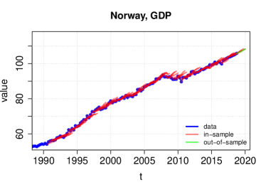
Figure 1: Five steps ahead in-sample (red) and out-of sample (green) forecasts for Norwegian GDP by the model (7) with elasticity constraint (8)

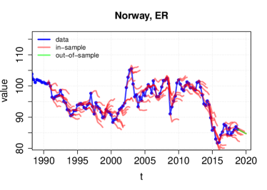
Figure 2: Five steps ahead in-sample (red) and out-of sample (green) forecasts for Norwegian real effective exchange rate by the model (7) with elasticity constraint (8)

Long-run the impulse responses to a positive shock in oil prices are positive for both the real exchange rate and real GDP. Improvement in the terms of trade leads to the exchange rate strengthening, which ensures internal and external equilibrium. This means that for the same volume of exports a country can buy a larger volume of imported goods. Therefore the prices of domestic non-tradable goods relative to prices of imported goods should increase to ensure the increase in the share of imported goods in aggregated consumption (Edwards, 1988). Furthermore the oil prices rise leads to an increase in GDP through the capital accumulation channel, namely, the higher oil prices result in new investment opportunities (Esfahani et al., 2014) and increase of domestic returns (Idrisov et al., 2015). The model indicates significant change in the short run transmission mechanism of oil prices shocks to the real exchange rate. IRFs for years 1991 and 2018 are statistically different. Before the Norges Bank turned to inflation targeting in 2001 the real exchange rate response had been strengthening gradually towards its long-run equilibrium after a shock in oil prices. Under the inflation targeting regime we see some overshooting of the real exchange rate. There is no sizable time variation in model parameters over the last decade, and the shape of the impulse response function for the real exchange rate stabilizes. Impulse response function for the real GDP changes very slightly during the entire period under review. The results of pseudo out-of-sample forecasting experiment in Table 1 show that the proposed TVP-VAR with time-invariant long-run multipliers outperforms the benchmark TVP-VAR without constraints. Thus reduction of degrees of freedom in TVP-VAR model helps to improve the forecasting accuracy. The proposed constrained TVP-VAR delivers smaller forecast errors than constant-parameter VAR for 1-3 steps-ahead forecasts and accuracy similar to VAR for 4-5 step-ahead forecasts.

Next we consider an example of Russian economy, were a transition towards the inflation targeting regime has started in 2014.

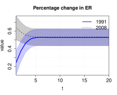
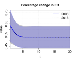
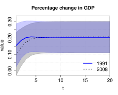
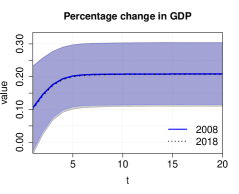
Figure 3: Norway. Impulse response functions for the proposed model: real exchange rate as a response variable

Figure 4: Norway. Impulse response functions for the proposed model: GDP as a response variable

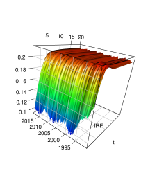
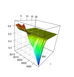
Figure 5: Norway. 3D impulse response functions for the proposed model: the impulse in oil prices and GDP (left) and real effective exchange rate (right) as response variables correspondingly

	Constrained			VAR			TVP-VAR (7)
steps	mean	std		mean	std		mean	std
GDP
1	0.60	0.61		1.02	0.79		1.02	0.80
2	0.95	0.84		1.07	0.89		1.08	0.90
3	1.16	1.04		1.26	1.01		1.26	0.97
4	1.39	1.25		1.45	1.15		1.40	1.12
5	1.62	1.39		1.61	1.27		1.55	1.26
ER
1	1.31	1.24		1.39	1.17		1.57	1.34
2	1.97	1.65		2.21	1.68		2.53	1.88
3	2.71	2.04		2.75	2.10		3.11	2.16
4	3.18	2.51		3.07	2.60		3.43	2.64
5	3.33	2.80		3.28	2.75		3.68	2.76

Table 1: Norway. Mean and standard deviation of absolute error of out-of-sample forecasts for the proposed method, TVP-VAR (7) with exogenous variables and VAR.

4.2 Russian economy

We use $93$ quarterly observations of real effective exchange rate of $S_{1,t}$, GDP $S_{2,t}$ for Russia and oil price $S_{x,t}$ from the 1st quarter 1995 till the 4th quarter 2018. A number of logarithm differences of observations of $y_{t}$ therefore was $92$. For the estimation of prior parameters of constrained TVP-VAR we used the first $t_{0}=40$ observations of $y_{i}^{t}$, $i=1,2$ and $x_{t}$. We selected an uninformative Gaussian prior for the elasticity $\theta\sim\mathcal{N}(\mu_{0},U_{0})$ (see Section 2.1) with $U_{0}={\rm diag}([0.1,0.1])$.

After $30000$ MCMC steps the estimating procedure for constrained TVP-VAR converged to $\theta=[0.09,\,0.04]^{\top}$, where the first component corresponds to real exchange rate and the second to GDP. Posterior median of VAR part of constrained TVP-VAR coefficients are shown in Figure 6, posterior medians of $D_{0,t}$ and $D_{1,t}$ are in Figure 7. The five-step ahead in-sample forecasts for the GDP and the real effective exchange rate (ER) along with out-of-sample forecast for the time interval $[2007\text{Q}_{4},2018\text{Q}_{4}]$ are shown in Figures 8, 9. Median of long-run growth rate with $60\%$ confidence intervals for GDP, which is the second component of $(I-B_{t})^{-1}c_{t}$, in percents is shown in Figure 10.

Figure 6: VAR coefficients in (7) with (8): first column corresponds to $c_{t}$, the next two columns show the behavior of the entries of $B_{t}$.

Figure 7: The dynamics of the entries of exogenous coefficients $D_{0,t}$ and $D_{1,t}.$

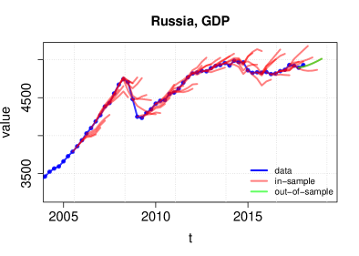
Figure 8: Five steps ahead in-sample (red) and out-of sample (green) forecasts for GDP by the model (7) with elasticity constraint (8)

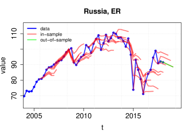
Figure 9: Five steps ahead in-sample (red) and out-of sample (green) forecasts for the real effective exchange rate by the model (7) with elasticity constraint (8).

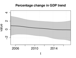
Figure 10: Percents of long-run growth rate of Russian GDP with $60\%$ confidence intervals

We compare impulse response functions for the years 2008 and 2018 for GDP and real exchange rate (ER) to the shock in exogenous logarithm of differences of oil prices. Results in Figs. 11 demonstrate the convergence to the same limiting value defined by (10); 3D-plots of impulse response functions are shown in Figs. 12. During the years before the crisis of 2008–2009 the Central Bank of Russia followed the policy of a managed nominal ruble exchange rate. From IRF for this period one can observe a gradual strengthening of the real exchange rate towards its long-run equilibrium after an increase in oil prices. During the next years the Central Bank of Russia switched to a floating exchange rate. After that the real exchange rate began to react to oil price shocks more sharply with the overshooting effect. It should be noted that during periods of gradual reaction of the exchange rate to the oil price shocks, real GDP reacted quite strongly to the shock. During the periods of sharp reaction of the real exchange rate the real GDP demonstrates gradual increase. Therefore our results are in line with a classical view: flexible exchange rates are shock absorbers for small open economies and the floating exchange rate regime of monetary policy reduces volatility of the GDP growth.

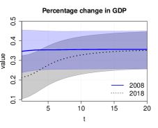
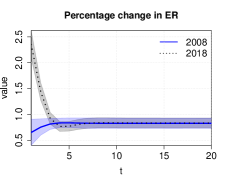
Figure 11: Impulse response functions for the proposed model: the impulse in oil and GDP and real exchange rate as response variable

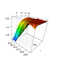
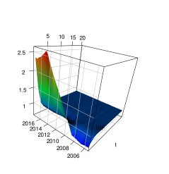
Figure 12: 3D impulse response functions for the proposed model: the impulse in oil and GDP (left) and real exchange rate (right) as response variables correspondingly

The mean absolute errors and standard deviations for of 1-5 steps out-of-sample forecasts of GDP and real exchange rate for the proposed method and benchmark methods for the time interval $[2007\text{Q}_{4},2019\text{Q}_{1}]$ are shown in Table 2. One may conclude that in terms of forecasts a classical VAR gives better result than TVP-VAR (Del Negro and Primiceri, 2015, Primiceri, 2005) extended for exogenous variables case. Imposing the elasticity constraint helps to improve the situation: the proposed method outperforms both benchmark methods in forecasting of GDP 1-3 steps ahead. The proposed method gives smaller forecasting error that non-constrained TVP-VAR for the real exchange rate. Nevertheless, the uncertainty coming from the coefficients model brings though delivers slightly less accuracy than VAR for the real exchange rate and 4-5 steps ahead forecasts of GDP. The results demonstrate that imposing the long run elasticity constraint allows to improve the quality of modeling. Figure 10 demonstrates significant decrease in the long-run growth rates for the Russian economy.

	Constrained			VAR			TVP-VAR (7)
steps	mean	std		mean	std		mean	std
GDP
1	28.01	41.46		46.37	50.81		51.02	56.58
2	61.58	79.01		79.97	97.29		98.21	110.71
3	91.24	116.77		105.50	124.53		120.59	148.80
4	119.06	147.81		120.42	141.74		135.97	167.98
5	155.03	166.91		133.42	158.50		150.30	180.91
ER
1	4.99	7.37		4.67	4.69		5.48	5.37
2	6.16	5.95		6.00	5.69		7.50	6.97
3	6.96	5.95		6.65	4.61		7.19	5.75
4	6.77	6.77		6.52	5.49		6.39	6.52
5	7.48	7.92		6.91	6.05		7.36	6.39

Table 2: Russia. Mean and standard deviation of absolute error of out-of-sample forecasts for the proposed method, TVP-VAR (7) with exogenous variables and VAR.

5 Conclusions

In the paper we propose a TVP-VAR model with a time-invariant constraint on the long-run multipliers of endogenous variables with respect to changes in exogenous variable. We provide a Bayesian estimation method for TVP-VAR parameters and multipliers. The proposed methodology can be used for a wide range of practical applications as an alternative to VARX, for example, in open economies modeling. Our approach is tailored to economic systems whose cross-correlation relationships change due to changes in the monetary policy and exchange rate regimes under the hypothesis of long-run money neutrality. In the modern New Keynesian models the particular monetary policy rule matters for the shape of transition path from one long-run equilibrium to another. However, usually there is no influence of the monetary policy rule on the long-run equilibrium. We apply the proposed methodology to model relationship between the real GDP, the real exchange rate and real oil prices for the Norwegian and the Russian economies. Results show that incorporating the time invariance constraint for the long-run multipliers significantly improves forecasting performance of TVP-VAR model. Impulse responses are interpretable. The oil price increase leads to statistically significant real exchange rate appreciation and GDP increase in long run. During periods of gradual reaction of the real exchange rate to the oil price shocks, real GDP reacted strongly to the shock. During periods of the sharp reaction of the real exchange rate, the real GDP demonstrates gradual increase. Therefore our results are in line with classical view that flexible exchange rates are shock absorbers for small open economies and the floating exchange rate regime of monetary policy reduces volatility of the GDP growth.

References

References

- Altig et al. (2011) Altig, D., Christiano, L.J., Eichenbaum, M., Linde, J., 2011. Firm-specific capital, nominal rigidities and the business cycle. Review of Economic dynamics 14, 225–247.
- Antolin-Diaz et al. (2017) Antolin-Diaz, J., Drechsel, T., Petrella, I., 2017. Tracking the slowdown in long-run gdp growth. Review of Economics and Statistics 99, 343–356.
- Baumeister and Peersman (2013) Baumeister, C., Peersman, G., 2013. Time-varying effects of oil supply shocks on the us economy. American Economic Journal: Macroeconomics 5, 1–28.
- Broda (2004) Broda, C., 2004. Terms of trade and exchange rate regimes in developing countries. Journal of International economics 63, 31–58.
- Canova and Pérez Forero (2015) Canova, F., Pérez Forero, F.J., 2015. Estimating overidentified, nonrecursive, time-varying coefficients structural vector autoregressions. Quantitative Economics 6, 359–384.
- Carter and Kohn (1994) Carter, C.K., Kohn, R., 1994. On gibbs sampling for state space models. Biometrika 81, 541–553.
- Chen (2009) Chen, S.S., 2009. Oil price pass-through into inflation. Energy Economics 31, 126–133.
- Clarida et al. (2000) Clarida, R., Gali, J., Gertler, M., 2000. Monetary policy rules and macroeconomic stability: evidence and some theory. The Quarterly journal of economics 115, 147–180.
- Clark and Doh (2014) Clark, T.E., Doh, T., 2014. Evaluating alternative models of trend inflation. International Journal of Forecasting 30, 426–448.
- Clark and Ravazzolo (2015) Clark, T.E., Ravazzolo, F., 2015. Macroeconomic forecasting performance under alternative specifications of time-varying volatility. Journal of Applied Econometrics 30, 551–575.
- Cogley (2005) Cogley, T., 2005. How fast can the new economy grow? a bayesian analysis of the evolution of trend growth. Journal of macroeconomics 27, 179–207.
- Cogley et al. (2010) Cogley, T., Primiceri, G.E., Sargent, T.J., 2010. Inflation-gap persistence in the us. American Economic Journal: Macroeconomics 2, 43–69.
- Cogley and Sargent (2001) Cogley, T., Sargent, T.J., 2001. Evolving post-world war ii us inflation dynamics. NBER macroeconomics annual 16, 331–373.
- Cogley and Sargent (2005) Cogley, T., Sargent, T.J., 2005. Drifts and volatilities: monetary policies and outcomes in the post wwii us. Review of Economic dynamics 8, 262–302.
- Cogley and Sbordone (2008) Cogley, T., Sbordone, A.M., 2008. Trend inflation, indexation, and inflation persistence in the new keynesian phillips curve. American Economic Review 98, 2101–26.
- Cross and Nguyen (2017) Cross, J., Nguyen, B.H., 2017. The relationship between global oil price shocks and china’s output: A time-varying analysis. Energy economics 62, 79–91.
- Cushman and Zha (1997) Cushman, D.O., Zha, T., 1997. Identifying monetary policy in a small open economy under flexible exchange rates. Journal of Monetary economics 39, 433–448.
- D’Agostino et al. (2013) D’Agostino, A., Gambetti, L., Giannone, D., 2013. Macroeconomic forecasting and structural change. Journal of applied econometrics 28, 82–101.
- Del Negro and Primiceri (2015) Del Negro, M., Primiceri, G.E., 2015. Time varying structural vector autoregressions and monetary policy: a corrigendum. The review of economic studies 82, 1342–1345.
- Edwards (1988) Edwards, S., 1988. Real and monetary determinants of real exchange rate behavior: Theory and evidence from developing countries. Journal of development economics 29, 311–341.
- Edwards and Yeyati (2005) Edwards, S., Yeyati, E.L., 2005. Flexible exchange rates as shock absorbers. European Economic Review 49, 2079–2105.
- Esfahani et al. (2014) Esfahani, H.S., Mohaddes, K., Pesaran, M.H., 2014. An empirical growth model for major oil exporters. Journal of Applied Econometrics 29, 1–21.
- Fernández et al. (2017) Fernández, A., Schmitt-Grohé, S., Uribe, M., 2017. World shocks, world prices, and business cycles: An empirical investigation. Journal of International Economics 108, S2–S14.
- Fisher and Seater (1993) Fisher, M.E., Seater, J.J., 1993. Long-run neutrality and superneutrality in an arima framework. The American Economic Review , 402–415.
- Gambetti et al. (2008) Gambetti, L., Pappa, E., Canova, F., 2008. The structural dynamics of us output and inflation: what explains the changes? Journal of Money, Credit and Banking 40, 369–388.
- Gelfand and Smith (1990) Gelfand, A.E., Smith, A.F., 1990. Sampling-based approaches to calculating marginal densities. Journal of the American statistical association 85, 398–409.
- Gelfand and Smith (1991) Gelfand, A.E., Smith, A.F., 1991. Gibbs sampling for marginal posterior expectations. Communications in Statistics-Theory and Methods 20, 1747–1766.
- Hamilton (1995) Hamilton, J.D., 1995. Time series analysis. Economic Theory. II, Princeton University Press, USA , 625–630.
- Idrisov et al. (2015) Idrisov, G., Kazakova, M., Polbin, A., 2015. A theoretical interpretation of the oil prices impact on economic growth in contemporary russia. Russian Journal of Economics 1, 257–272.
- Judd et al. (1998) Judd, J.P., Rudebusch, G.D., et al., 1998. Taylor’s rule and the fed: 1970-1997. Economic Review-Federal Reserve Bank of San Francisco , 3–16.
- Justiniano and Primiceri (2008) Justiniano, A., Primiceri, G.E., 2008. The time-varying volatility of macroeconomic fluctuations. American Economic Review 98, 604–41.
- Kang et al. (2009) Kang, K.H., Kim, C.J., Morley, J., 2009. Changes in us inflation persistence. Studies in Nonlinear Dynamics & Econometrics 13.
- Kim and Nelson (1999) Kim, C.J., Nelson, C.R., 1999. Has the us economy become more stable? a bayesian approach based on a markov-switching model of the business cycle. Review of Economics and Statistics 81, 608–616.
- Kim et al. (1998) Kim, S., Shephard, N., Chib, S., 1998. Stochastic volatility: likelihood inference and comparison with arch models. The review of economic studies 65, 361–393.
- King and Watson (1992) King, R., Watson, M.W., 1992. Testing long run neutrality. Technical Report. National Bureau of Economic Research.
- Koop and Korobilis (2013) Koop, G., Korobilis, D., 2013. Large time-varying parameter vars. Journal of Econometrics 177, 185–198.
- Krueger (2015) Krueger, F., 2015. bvarsv: Bayesian analysis of a vector autoregressive model with stochastic volatility and time-varying parameters. Https://CRAN.R-project.org/package=bvarsv.
- Kruse and Wegener (2019) Kruse, R., Wegener, C., 2019. Time-varying persistence in real oil prices and its determinant. Energy Economics Forthcoming.
- Levy-Yeyati and Sturzenegger (2005) Levy-Yeyati, E., Sturzenegger, F., 2005. Classifying exchange rate regimes: Deeds vs. words. European economic review 49, 1603–1635.
- Lubik and Schorfheide (2004) Lubik, T.A., Schorfheide, F., 2004. Testing for indeterminacy: An application to us monetary policy. American Economic Review 94, 190–217.
- Lucas et al. (1976) Lucas, R.E., et al., 1976. Econometric policy evaluation: A critique, in: Carnegie-Rochester conference series on public policy, pp. 19–46.
- Mavroeidis (2010) Mavroeidis, S., 2010. Monetary policy rules and macroeconomic stability: some new evidence. American Economic Review 100, 491–503.
- McConnell and Perez-Quiros (2000) McConnell, M.M., Perez-Quiros, G., 2000. Output fluctuations in the united states: What has changed since the early 1980’s? American Economic Review 90, 1464–1476.
- Peersman (2005) Peersman, G., 2005. What caused the early millennium slowdown? evidence based on vector autoregressions. Journal of Applied Econometrics 20, 185–207.
- Primiceri (2005) Primiceri, G.E., 2005. Time varying structural vector autoregressions and monetary policy. The Review of Economic Studies 72, 821–852.
- Riggi and Venditti (2015) Riggi, M., Venditti, F., 2015. The time varying effect of oil price shocks on euro-area exports. Journal of Economic Dynamics and Control 59, 75–94.
- Sims and Zha (2006) Sims, C.A., Zha, T., 2006. Were there regime switches in us monetary policy? American Economic Review 96, 54–81.
- Stock and Watson (2007) Stock, J.H., Watson, M.W., 2007. Why has us inflation become harder to forecast? Journal of Money, Credit and banking 39, 3–33.
- Uribe and Yue (2006) Uribe, M., Yue, V.Z., 2006. Country spreads and emerging countries: Who drives whom? Journal of international Economics 69, 6–36.
- Weber (1994) Weber, A.A., 1994. Testing long-run neutrality: empirical evidence for g7-countries with special emphasis on germany, in: Carnegie-Rochester Conference Series on Public Policy, Elsevier. pp. 67–117.