pnasresearcharticle This paper sheds light on the phase portrait structure of a ’minimal model’ for a large nonlinear system of many randomly interacting degrees of freedom equipped with a stability feedback mechanism. In this way it significantly extends local stability analysis of large complex systems which was undertaken by Robert May in 1972. We show that the transition from stability to instability is characterized by the exponential explosion in the number of unstable equilibria, with drastically reduced probability of finding truly locally attracting equilibria . At the same time we demonstrate abundance of equilibria with a large proportion of stable directions, which arguably can slow down the system dynamics for sufficiently long time and induce aging effects. (1) Author contributions: G.B.A., Y.V.F. and B.A.K. performed research and wrote the paper The authors declare no conflict of interest. Corresponding Authors:
benarous@cims.nyu.edu, yan.fyodorov@kcl.ac.uk, b.khoruzhenko@qmul.ac.uk

Counting equilibria of large complex systems by instability index

Abstract

We consider a nonlinear autonomous system of $N\gg 1$ degrees of freedom randomly coupled by both relaxational (’gradient’) and non-relaxational (’solenoidal’) random interactions. We show that with increased interaction strength such systems generically undergo an abrupt transition from a trivial phase portrait with a single stable equilibrium into a topologically non-trivial regime of ’absolute instability’ where equilibria are on average exponentially abundant, but typically all of them are unstable, unless the dynamics is purely gradient. When interactions increase even further the stable equilibria eventually become on average exponentially abundant unless the interaction is purely solenoidal. We further calculate the mean proportion of equilibria which have a fixed fraction of unstable directions.

This manuscript was compiled on

In 1972, in his seminal paper (1) Robert May analyzed the relationship between complexity and stability of large complex systems at equilibrium. Although May was motivated by the "stability versus diversity" debate in ecology (2), his neighborhood stability analysis applies far beyond model ecology, e.g., to neural networks (3, 4), systemic risk in trading (5) or modeling of large economies (6). To recap it, consider a system of $N\gg 1$ degrees of freedom ${x}=(x_{1},\ldots,x_{N})^{T}$, whose evolution is governed by a set of coupled non-linear first-order ordinary differential equations. The local stability analysis of an equilibrium, say ${x}_{*}$, amounts to linearizing the system near ${x}_{*}$ and looking at the time evolution of the displacement ${y}={x}-{x}_{*}$. Assuming that each of the degrees of freedom $x_{i}$ by itself, when disturbed from equilibrium, returns back with some characteristic time independent of $i$, such evolution is described by the equation $\dot{{y}}=-\mu{y}+J{y}$. Here, the parameter $\mu>0$ sets the characteristic relaxation time in the absence of interactions and the matrix $J=(J_{ij})$ describes the pair-wise interactions between the degrees of freedom in the neighborhood of ${x}_{*}$.

To get insights into the interplay between stability and complexity, May simplified the problem by assuming that positive and negative values of the pair-wise interactions $J_{ij}$ are equally likely to occur, a plausible assumption for large complex systems. Accordingly, he chose $J_{ij}$ to be random variables with zero mean and standard deviation $\sigma$ (‘typical’ interaction strength), thus retaining the fewest possible number of control parameters in his model. Invoking random matrix theory, he then concluded that large complex systems exhibit a sharp transition from stability to instability when the number of degrees of freedom or the interaction strength increase beyond the instability threshold which is given by a remarkably simple equation $\mu=\sigma\sqrt{N}$.

One obvious limitation of the neighborhood stability analysis is that it gives no insight into what happens outside the immediate neighborhood of equilibrium when it becomes unstable. Hence, May’s analysis has only limited bearing on the dynamics of populations operating out-of-equilibrium (2). For example, in the context of model ecosystems, populations may coexist thanks to limit cycles or chaotic attractors, which typically originate from unstable equilibrium points. This naturally prompts important lines of enquiry for large complex systems about classification of equilibria by stability, studying basins of attraction, and other features of global dynamics.

In an extension of May’s work, two of us introduced a ‘minimal’ nonlinear model of large complex systems equipped with a stability feedback mechanism (7). The main finding of (7) was that such systems exhibit a transition from a trivial phase portrait with a single stable equilibrium to one characterized by exponentially many equilibria. However, the important question about stability of those exponentially many equilibria remained unanswered. In the present paper we develop a framework for a statistical description of equilibria of large complex systems and then use it to calculate frequencies of stable equilibria and, also, of equilibria with a fixed fraction of stable directions.

Statistics of unstable equilibria with a large fraction of stable directions are of a particular interest in the context of large complex systems with an underlying energy landscape. In that case the dynamics can be visualized as a gradient descent on the energy surface, and, as was argued in ref. (8) the system is trapped near borders (ridges) of basins of attraction of local minima because of the dominance of borders in large-dimensional spaces. The gradient descent is then determined mainly by nearby saddles which lie on the ridges, which may trap dynamics for a long time due to the large number of stable directions. It is natural to expect that unstable equilibria with a large number of attracting directions may play a similar role in non-gradient dynamics, providing a motivation for our research.

Statistics of equilibria

The model studied in (7) is described by a system of autonomous non-linear differential equations

$$\dot{{x}}=-\mu{x}+{f}({x}),\quad{x}\in\mathbb{R}^{N},$$ (1)

coupled via a smooth random vector field ${f}({x})$ which models both the complexity and nonlinearity of interactions. Finding equilibria, i.e. solutions of Eq. 1 which do not change with time, amounts to solving the equation $-\mu{x}+{f}(\mathbf{x})=0$. Since the interaction field ${f}({x})$ is random, the total number of equilibria and their locations are not fixed in our model and may change from one realization of ${f}({x})$ to another. Thus, in contrast to the neighborhood stability analysis of a known equilibrium which was carried out by May, our model does not provide insights into properties of a single given equilibrium. Instead it makes possible a statistical analysis of stability properties of equilibria. Effectively, May’s question “Will a large complex system be stable” in our model is replaced by the question "What is the probability that an equilibrium drawn at random from the entire population of equilibria is stable?"

This probability, denote it by $p_{st}$, can be written in terms of counting statistics of equilibria. If ${\cal N}_{eq}$ is the total number of equilibria and ${\cal N}_{st}$ is the number of stable equilibria, then one can argue, see below, that

$$p_{st}=\langle{\cal N}_{st}/{\cal N}_{eq}\rangle\,,$$ (2)

where the angle brackets stand for averaging over ${f}({x})$.

Both counting functions, ${\cal N}_{eq}$ and ${\cal N}_{st}$, are examples of linear statistics of equilibria of the form

$$L[\mathit{\Psi}]=\sum_{{x}_{*}}\!\!\mathit{\Psi}({x}_{*})$$

where the sum is over all equilibria and $\Psi$ is a test function. In these notations, ${\cal N}_{eq}=L[1]$ and ${\cal N}_{st}=L\big{[}\mathit{\Theta}(\mu-x_{max}(J))\big{]}$, where $J$ is the Jacobian matrix $({\partial f_{i}}/{\partial x_{j}})$ of the vector field ${f}({x})$, $x_{max}(J)$ is the largest real part of the eigenvalues of $J$ and $\mathit{\Theta}(x)$ is the Heaviside step function, so that $\mathit{\Theta}(\mu-x_{max}(J))$ is the indicator-function of the event that $x_{max}(J)<\mu$.

The test function $\mathit{\Psi}_{J}\!=\!\delta(J\!-\!({\partial f_{i}}/{\partial x_{j}}))$, where $\delta(J)$ is the matrix delta-function provides another example of linear statistics of equilibria. Its weighted average,

$$P_{eq}(J)=\big{\langle}\frac{1}{{\cal N}_{eq}}\sum_{{x}_{*}}\prod_{i,j}\delta\big{(}J_{ij}-\frac{\partial f_{i}}{\partial x_{j}}({x}_{*})\big{)}\big{\rangle}\,,$$

is the sample mean of the joint probability density function for the matrix elements $J_{ij}$ of the Jacobian at equilibrium. Then, the probability for a randomly selected equilibrium point to be stable is $p_{st}\!=\!\int\!\!\mathit{\Theta}(\mu\!-\!x_{max}(J))P_{eq}(J)\,dJ\,.$ On replacing $P_{eq}(J)$ here with its expression in terms of the weighted average above, one immediately obtains Eq. 2.

One can extend this statistical framework from the binary descriptor of points of equilibria (stable or unstable) to a continuous one. Define $\kappa({x}_{*})$ to be the dimension of the local unstable manifold of the non-linear system [1] at equilibrium ${x}_{*}$, i.e., $\kappa({x}_{*})$ is the number of eigenvalues of the matrix $-\mu\delta_{ij}+\frac{\partial f_{i}}{\partial x_{j}}$ at ${x}={x}_{*}$ with positive real parts. In the limit $N\gg 1$, the fraction $\kappa({x}_{*})/N$ can be interpreted as a measure of instability of the equilibrium at ${x}_{*}$. We shall call an equilibrium $\alpha$-stable if its instability index $\kappa/N$ does not exceed value $\alpha$ and denote by ${\cal N}_{st}^{(\alpha)}$ the number of $\alpha$-stable equilibria. Then the probability that an equilibrium drawn at random from the entire population of equilibria will have its instability index in the interval $(\alpha_{1},\alpha_{2})$ is $\int_{\alpha_{1}}^{\alpha_{2}}\nu({\alpha})\,d\alpha$, where

$$\nu({\alpha})={dp_{\alpha}}/{d\alpha},\quad p_{\alpha}=\langle{\cal N}_{st}^{(\alpha)}\!/{\mathcal{N}_{eq}}\rangle\,.$$ (3)

The counting function ${\cal N}_{st}^{(\alpha)}$ can too be cast in the framework of linear statistics of equilibria. To this end, let us order the eigenvalues $z_{j}$ of the Jacobian matrix $J=({\partial f_{i}}/{\partial x_{j}})$ by their real parts $x_{j}=\operatorname{Re}z_{j}$ so that $x_{max}=x_{1}\geq x_{2}\geq\ldots\geq x_{N}$. Then ${\cal N}_{st}^{(\alpha)}=L[\mathit{\Theta}(\mu-x_{\alpha N+1})]$.

The computation of $p_{st}$ and $\nu(\alpha)$ is a challenging problem. Instead, in this paper we study their ‘annealed’ versions,

$$p^{(a)}_{st}=\frac{\langle{\cal N}_{st}\rangle}{\langle{\cal N}_{eq}\rangle},\quad\nu^{(a)}_{N}(\alpha)=\frac{1}{\langle\mathcal{N}_{eq}\rangle}\frac{d}{d\alpha}\langle\mathcal{N}^{(\alpha)}_{st}\rangle\,,$$ (4)

thus reducing the problem to calculating the expected number of stable and $\alpha$-stable equilibria. These are interesting observables on their own. As we shall shaw below the corresponding annealed complexity exponents, see Eq. 11, which can be computed in a closed form in the limit of large number of degrees of freedom, exhibit not-trivial dependences on the model parameters. Also, in the particular case of gradient flow $\dot{{x}}=-\nabla L({x})$, the annealed complexity exponents of local minima and other stationary points on the (random) surface of the potential function $L({x})$ attracted considerable recent interest and especially in the context of glassy dynamics. Still, the question of whether the annealed probabilities [4] give any insight into their quenched counterparts [3] is an important open question. The recent progress (9, 10, 11) in understanding this question in the context of gradient dynamics on the energy surface of the $p$-spin spherical model gives rise to a hope that for some classes of coupling fields in [1] the annealed picture will resemble the quenched one. The task of identifying such classes of coupling fields is a challenging open problem which deserves further investigation along with the companion question about the qualitative differences between the quenched and annealed pictures.

Model assumptions

To get insights into statistics of equilibria of large complex systems, we follow the philosophy of the ’‘minimal’ model (7) and decompose the coupling field into the sum of gradient (curl-free) and solenoidal (divergence-free) components:

$$f_{i}({x})=-\frac{\partial V({x})}{\partial x_{i}}+\frac{1}{\sqrt{N}}\sum_{j=1}^{N}\frac{\partial A_{ij}({x})}{\partial x_{j}},\;i=1,\ldots,N,$$ (5)

where the matrix $A({x})$ is antisymmetric: $A_{ij}({x})=-A_{ji}({x})$ for every ${x}$. Such a representation provides a rich, though not most general, class of vector fields The scalar and vector potentials, $V({x})$ and $A({x})$ respectively, are assumed to be statistically independent, zero mean Gaussian random fields, with smooth realizations and the additional assumptions of homogeneity (translational invariance) and isotropy (rotational invariance):

$$\langle V({x})V({y})\rangle \!\!\!=\!\!\! v^{2}\mathit{\Gamma}_{V}\!\left(|{x}-{y}|^{2}\right)\,,$$ (6)

$$\langle A_{ij}({x})A_{nm}({y})\rangle \!\!\!=\!\!\! a^{2}\mathit{\Gamma}_{A}\!\left(|{x}-{y}|^{2}\right)\!(\delta_{in}\delta_{jm}\!-\!\delta_{im}\delta_{jn})\,.$$ (7)

The covariance functions, $\mathit{\Gamma}_{V}$ and $\mathit{\Gamma}_{A}$ are normalised by the condition $\frac{d^{2}}{ds^{2}}\mathit{\Gamma}_{V,A}(s)\left|{}_{s=0}\right.=1$. The covariance functions of isotropic Gaussian fields were first studied in (12). In particular, for $\mathit{\Gamma}\left(|{x}-{y}|^{2}\right)$ to define a covariance function in all dimensions $\mathbb{R}^{N}$ it must hold that $\mathit{\Gamma}(t)=\int_{0}^{\infty}\exp({-st})dG(s)$, $\forall t\geq 0$, for some finite measure $dG(s)$ on $\mathbb{R}_{+}$.

Our model has the fewest possible number of parameters. These are

$$\tau=\frac{v^{2}}{v^{2}+a^{2}}\quad\mbox{and}\quad m=\frac{\mu}{\sqrt{4N(v^{2}+a^{2})}}.$$ (8)

The scaled relaxation strength $m$ is a measure of the strength of the stability feedback mechanism relative to the interaction strength and the potentiality parameter $\tau$ controls the balance between the gradient and solenoidal components of the interaction. If $\tau=1$ then the flow defined by Eq. 1 is purely gradient: $\dot{{x}}=-\nabla L({x})$, with $L({x})=\mu|{x}|^{2}/2-V({x})$ being the associated Lyapunov function. And if $\tau=0$ then the interaction field ${f}({x})$ is divergence free.

Note that $m$ is essentially the same control parameter as one in May’s linear model. In the non-linear setting, it controls the complexity of the phase portrait. As was shown in ref. (7), for large values of $m$ the stability feedback mechanism prevails and, typically, the system has a single equilibrium which is stable. When the value of $m$ decreases, the system exhibits a sharp transition from this simple phase portrait to a complex one which is characterized by exponentially growing number of equilibria. More precisely, to leading order in the limit $N\gg 1$,

$$\langle{\cal N}_{eq}\rangle=\begin{cases}1,&\mbox{if }m>1,\\[4.30554pt] \sqrt{\frac{2(1+\tau)}{1-\tau}}\,e^{N\mathit{\Sigma}_{eq}(m)}\,,&\mbox{if }0<m<1\,,\end{cases}$$ (9)

where

$$\mathit{\Sigma}_{eq}(m)=\frac{1}{2}(m^{2}-1)-\ln m\,.$$

Thus, as far as the total number of equilibria is concerned, the picture that is emerging in the limit $N\gg 1$ is largely independent of $\tau$, although the pre-exponential factor in Eq. 9 suggests that the case of pure gradient flow $\tau=1$ is special .

The role of potentiality parameter $\tau$ will be revealed by our subsequent analysis.

Coming back to our model assumptions, one can use a different class of coupling fields $f(x)$ - homogenous Gaussian fields with zero mean and covariance

$$\langle f_{i}({x})f_{j}({y})\rangle=\mathit{\Gamma}_{1}(|x-y|^{2})\delta_{ij}+\mathit{\Gamma}_{2}(|x-y|^{2})(x_{i}-y_{i})(x_{j}-y_{j})\,.$$

This class of random fields have been used in the statistical theory of isotropic turbulence since 1930s (22, 23) and in the context of large complex systems very recently in ref. (24). Although such fields have a different covariance structure to the one given by Eqs 6–7, our stability analysis extends to this class almost verbatim.

One can also consider inhomogenous coupling fields, see ref. (25). As far as the assumptions of isotropy and Gaussianity of the coupling field ${f}({x})$ are concerned, recent progress in the evaluation of the rate of growth of random determinants of large random matrices with non-invariant matrix distribution (26, 27) raise hope that the isotropy assumption could be relaxed, at least in the gradient case. However, the Gaussianity assumption is indispensable. This assumption allows one to compute the Kac-Rice integral via its reducing to conditional averages of random matrix determinants, see Materials and Methods, and without it an effective computation of the Kac-Rice integral, Eq. [16], seems hardly possible.

Stable equilibria and stable directions of unstable equilibria

The starting point of our analysis of stability properties of equilibria is the Kac-Rice formula for counting solutions of simultaneous equations. By expressing the mean value of linear statistics of equilibria $\langle L[\mathit{\Psi}]\rangle$ as a random matrix average, it brings the original counting problem into the realms of random matrix theory, see ref. (7). If $\mathit{\Psi}({x}_{*})=\psi(J_{*})$, where $J_{*}=({\partial f_{i}}/{\partial x_{j}})$ is the Jacobian matrix of the interaction field ${f}({x})$ at ${x}={x}_{*}$, then (see Section Materials and Methods)

$$\langle L[\mathit{\Psi}]\rangle_{{f}}=\mu^{-N}\langle\psi(J)\,|\!\det(-\mu I+J)|\rangle_{J}\,.$$ (10)

Here the angle brackets on the left-hand side stand for the averaging over realizations of the interaction field ${f}({x})$, and the angle brackets on the right-hand side stand for the averaging over the distribution of the Jacobian matrix $J$. The latter does not depend of ${x}$ because of the homogeneity of ${f}({x})$.

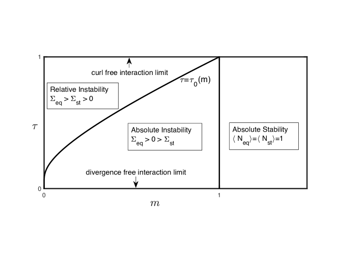
Figure 1: Phase diagram of model [1]. The curve $\tau=\tau_{0}(m)$ separates the regions of absolute and relative instability in the ‘topologically non-trivial’ phase.

Eq. 10 makes it possible to draw on analytic techniques from random matrix theory and compute counting statistics of equilibria, such as the complexity exponent $\mathit{\Sigma}_{eq}(m)$ associated with the total number of equilibria. In this context, powerful tools of Large Deviation Theory developed for matrices with complex eigenvalues in refs. (28, 29) become especially useful. They allow one to compute the complexity exponents $\mathit{\Sigma}_{st}$ and $\mathit{\Sigma}^{(\alpha)}_{st}$ associated with the stable and $\alpha$-stable equilibria:

$$\mathit{\Sigma}_{st}=\lim_{N\to\infty}\frac{1}{N}\ln\langle{\cal N}_{st}\rangle,\quad\mathit{\Sigma}^{(\alpha)}_{st}=\lim_{N\to\infty}\frac{1}{N}\ln\langle{\cal N}_{st}^{(\alpha)}\rangle\,.$$ (11)

One outcome of this computation (see Supplemental Information) is a closed form expression for $\mathit{\Sigma}_{st}$ in the topologically nontrivial phase:

$$\mathit{\Sigma}_{st}(m;\tau)=\mathit{\Sigma}_{eq}(m)-\frac{1+\tau}{2\tau}(1-m)^{2},\quad 0<m<1.$$ (12)

As a function of parameters $m$ and $\tau$, the complexity exponent $\mathit{\Sigma}_{st}$ is positive above the curve $\tau=\tau_{0}(m)$ in the $(m,\tau)$-plane,

$$\tau_{0}(m)=-\frac{1}{2}\frac{(1-m)^{2}}{{1-m+\ln{m}}},\quad 0\leq m\leq 1\,,$$ (13)

and is negative below. Thus, this curve and the vertical line $m=1$ partition the parameter space of our model into three regions, see Fig. 1. If $m>1$ the nonlinear system [1] has, on average, exactly one equilibrium and this equilibrium is stable. This is a region of absolute stability. If $m<1$ then the number of stable equilibria depends on the relative strength of curl-free and divergence-free components of the interaction field. If $\tau<\tau_{0}(m)$ then the complexity exponent $\mathit{\Sigma}_{st}$ is negative and the probability that the system has at least one stable equilibrium is exponentially small for large $N$. This is a region of absolute instability: on average, equilibria are exponentially abundant but only very rare realizations of the interaction field yield stable equilibria. In contrast, if $\tau>\tau_{0}(m)$ then the complexity exponent $\mathit{\Sigma}_{st}$ is positive, so that in this region the stable equilibria are, on average, exponentially abundant. However, $\mathit{\Sigma}_{st}<\mathit{\Sigma}_{eq}$ and, hence, the stable equilibria are, on average, exponentially rare among all equilibria. This is also reflected in the fact that if $m<1$ then the probability for an equilibrium to be stable is, in the annealed approximation, exponentially small for $N$ large regardless of the value of $\tau$: to leading order in $N$,

$$\ln p_{st}^{(a)}=-N(1+\tau)(1-m)^{2}/(2\tau).$$

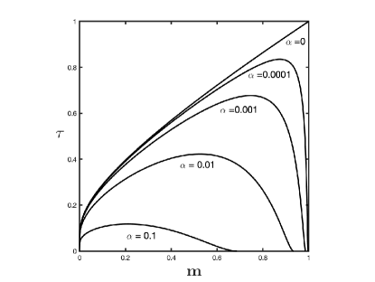
Figure 2: The graph of $\tau_{0}^{(\alpha)}(m)$ as function of $m$ for $\alpha=0,0.1,0.01,0.001$ and 0.0001, $\tau_{0}^{(0)}(m)=\tau_{0}(m)$.

One can also compute in closed form the complexity exponent associated with the $\alpha$-stable equilibria. The result of this computation is that $\mathit{\Sigma}_{st}^{(\alpha)}(m,\tau)=\mathit{\Sigma}_{eq}(m)$ for all $\alpha\geq 1/2$ and that for all $0\leq\alpha\leq 1/2$,

$$\mathit{\Sigma}_{st}^{(\alpha)}(m,\tau)=\begin{cases}\displaystyle{\mathit{\Sigma}_{eq}(m)-\frac{1+\tau}{2\tau}(m_{\alpha}-m)^{2}},&0<m\leq m_{\alpha},\\ \mathit{\Sigma}_{eq}(m),&m_{\alpha}\leq m<1,\end{cases}$$

where $m_{\alpha}$ is the solution of equation

$$\alpha=\frac{1}{\pi}\big{(}\arccos{m}-m\sqrt{1-m^{2}}\big{)}$$ (14)

for $m$. The zero-level line of $\mathit{\Sigma}^{(\alpha)}_{st}$, $\tau=\tau_{0}^{(\alpha)}(m)$, is given by

$$\tau_{0}^{(\alpha)}(m)=\frac{(m_{\alpha}-m)^{2}}{-1-m_{\alpha}^{2}-2\ln{m}+2mm_{\alpha}},\quad 0\leq m\leq m_{\alpha}\,.$$

The striking feature that emerges from our analysis is the abundance of unstable equilibria with a large proportion of stable directions even far inside the absolute instability region. A quick inspection of Fig. 2 leads to the conclusion that even though below the line $\tau=\tau_{0}(m)$ the probability for the system to have at least one stable equilibrium is exponentially small, equilibria with a large proportion of stable directions are in abundance in this parameter range. This surprising feature can be visualized in the following way. For every point $(m,\tau)$ below the line $\tau=\tau_{0}(m)$ there is a unique value of $\alpha$ such that the zero-level line of $\mathit{\Sigma}^{(\alpha)}_{st}$ passes through this point. This mapping $(m,\tau)\to\alpha$ defines a function $\alpha(m,\tau)$ which we extend into the region above the line $\tau=\tau_{0}(m)$ by setting $\alpha(m,\tau)\equiv 0$ everywhere in this region. The heat map of $\alpha(m,\tau)$, the plot on the left-hand side in Fig. 3, reveals that there is not much difference between points above and below the critical line $\tau=\tau_{0}(m)$ apart from a small area near $\tau=0$. For example, the zero-level lines of $\mathit{\Sigma}^{(\alpha)}_{st}$ are barely visible (compare Fig. 2 and the plot on the left-hand side in Fig. 3). One only recovers zero-level lines $\tau=\tau^{(\alpha)}(m)$ from the heat map of $\ln\alpha(m,\tau)$, see the plot on the right-hand side in Fig. 3.

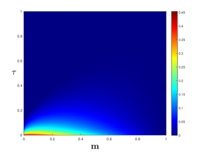
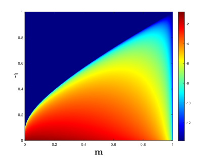
Figure 3: The heat maps of $\alpha(m,\tau)$ (plot on the left-hand side) and $\ln\alpha(m,\tau)$ (plot on the right-hand side).

To clarify the last point and to get a coherent understanding of the arising picture of indices associated with equilibria in our system it is helpful to consider the relative density $\nu_{N}^{(a)}\!({\alpha})$ of $\alpha$-stable equilibria, see Eq. 4. This is the probability density function of instability index $\alpha$ in the annealed approximation. Namely, the probability that an equilibrium drawn at random from the entire population of equilibria will have its instability index in the interval $(\alpha_{1},\alpha_{2})$ is given by the integral $\int_{\alpha_{1}}^{\alpha_{2}}\nu_{N}^{(a)}({\alpha})\,d\alpha$ in the annealed approximation. In the limit $N\gg 1$ this density can be determined in closed form in the entire range of $\alpha\in[0,1]$, including the leading pre-exponential factor, see Supplementary Information. To leading order in $N$,

$$\nu_{N}^{(a)}({\alpha})=\frac{1}{2}\sqrt{\frac{N\pi(1+\tau)}{2\tau(1-m^{2})}}\,e^{-\frac{1+\tau}{2}\big{[}\!\frac{\sqrt{N}(m_{\alpha}-m)}{\sqrt{\tau}}\big{]}^{2}},$$ (15)

where, for any given $\alpha\in[0,1]$, $m_{\alpha}$ is the (unique) solution of Eq. 14 for $m$ in the interval $[-1,1]$. It is apparent that in the topologically non-trivial phase $m\in(0,1)$ only equilibria with the instability indices $\alpha$ in a narrow interval of width $\sqrt{\tau/N}$ around the value $\alpha_{m}=\frac{1}{\pi}[\arccos{m}-m\sqrt{1-m^{2}}]$, $0\leq\alpha_{m}\leq 1/2$, have finite density, see Fig. 4. The equilibria with index $\alpha>1/2$ have, on average, always exponentially vanishing density relative to the total number of equilibria. This can be seen by noticing that $m_{\alpha}$ is negative for such values of $\alpha$.

The transition from absolute stability to instability as the system complexity increases is very sharp for $N$ large. Indeed, the complexity exponent $\mathit{\Sigma}_{eq}(m)$ vanished quadratically at $m=1$, hence the width of the transition region scales as $N^{-\frac{1}{2}}$. Although our methods give no access to the entire transition region one can probe its left tail by setting

$$m=1-{\delta}/\sqrt{N},\quad 1\ll\delta\ll\sqrt{N}.$$

in Eqs 12 – 15. For example, the probability for an equilibrium to have the number of its unstable directions $\kappa$ in the interval $(\gamma_{1}N^{1/4},\gamma_{2}N^{1/4})$ is given, in the annealed approximation, by $\int_{\gamma_{1}}^{\gamma_{2}}\sigma(\gamma)\,d\gamma$ where to leading order in $N$ and $\delta$

$$\sigma(\gamma)\!=\!\frac{1}{N^{3/4}}\nu^{(a)}\!\Big{(}\frac{\gamma}{N^{3/4}}\!\Big{)}=\sqrt{\frac{\pi(1+\tau)}{16\,\tau\delta}}e^{-\frac{1+\tau}{2\tau}\big{[}\delta-\frac{1}{2}\big{(}\frac{3\pi}{2}\gamma\big{)}^{2/3}\big{]}^{2}},$$

see Supplemental Information. In particular, this means that in the left tail of the transition region the number of unstable directions of a typical equilibrium scales with $N$ as $N^{1/4}$. This leads to the natural conjecture that the number of unstable directions of typical equilibria in the entire transition region is proportional to $N^{1/4}$. In the annealed approximation this conjecture was verified in ref (30) for the pure gradient flow.

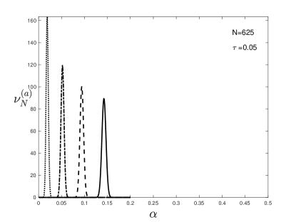
Figure 4: Plot of the relative density of instability index of typical equilibria $\nu^{(a)}_{N}(\alpha)$ for $N=625$ and $m=0.9$ (dotted line), $m=0.8$ (dash-dotted line), $m=0.7$ (dashed line) and $m=0.6$ (solid line). $\tau=0.8$ in the plot on the left-hand side and $\tau=0.05$ in the plot on the right-hand side. Note that typical equilibria have high proportion of stable directions even when the system complexity is relatively large.

Discussion

In this paper we extend May’s local stability analysis of large complex systems from the neighborhood of a single equilibrium to the entire phase space of the system. The systems which we consider are equipped with a stability feedback mechanism and the interaction complexity is modeled by a random field of zero mean value which couples the degrees of freedom, see Eq. 1. Our model system is, in a certain sense, ’minimal’ as it has only two control parameters, see Eq. 8.

The following picture then emerges from our analysis. For large values of $m$ the stability feedback mechanism prevails and, typically, large complex systems will have only one equilibrium which is stable. This is the regime of absolute stability. For non-gradient systems ($\tau<1$), as the interaction strength increases the system undergoes a sharp transition at the critical point $m=m_{C}=1$ from the regime of absolute stability to the regime of absolute instability. In latter regime the system has multiple equilibria, but the probability for the system to have at least one stable equilibrium is exponentially small. However, equilibria with a large proportion of stable directions are in abundance in this regime. With the further increase of the interaction strength, the system transits to the regime of relative instability which is characterized by the abundance of stable equilibria, yet the unstable equilibria dominate. The transition point $m=m_{B}$ from the absolute to relative instability depends on the relative strength of the stability feedback mechanism and the balance between the gradient and solenoidal components of the coupling field, see Eq. 13, and if the coupling is divergence-free ($\tau=0$) then the relative stability regime does not exists at all. If the coupling is curl-free ($\tau=1$) then, as the interaction strength increases, the system transits from the regime of absolute stability directly to the regime of relative instability.

We expect that some qualitative features revealed in the phase portrait of the present model may be shared by other systems of randomly coupled autonomous ODE’s with large number of degrees of freedom, such as e.g. a model of neural network consisting of randomly interconnected neural units (4), or non-relaxational version of the spherical spin-glass model (31, 32). Earlier studies, starting from the classical paper (3) suggested that autonomous dynamics in the ’topologically nontrivial’ regime should be predominantly chaotic, see (4, 33) and references therein. The absence of stable, attracting equilibria certainly corroborates this conclusion, though presence of stable periodic orbits in the phase space can not be excluded on those grounds either. The influence of the non-gradient component of the vector field on system dynamics needs further clarification as well. On one hand, as we discovered above any admixture of such components very efficiently eliminates all stable equilibria when entering the ’topologically non-trivial’ regime. On the other hand, the results of the paper (32) suggest that the influence of such non-potentiality on long-time ’aging’ effects in dynamics of glassy-type models is relatively benign. This may imply that the dynamical dominance of exponentially abundant, though unstable equilibria with yet extensively many stable directions may be enough for ’trapping’ the system dynamics for a long time in the vicinity of such equilibria, thus inducing aging phenomena similar to the gradient descent case (8, 34).

As one of main outstanding challenges one must mention obtaining statistical characteristics of ${\cal N}_{eq}$ and ${\cal N}_{st}$ beyond their mean values. As it is known that ”quenched” and ”annealed” complexity of minima may not coincide in some models of random landscapes, see e.g. (17, 9), one may expect that such a calculation may lead to a further refinement of the picture of transition lines presented in our paper for certain classes of random functions $V({x})$ and $A_{ij}({x})$. Recent progress in purely gradient case is encouraging, see (9, 20) and hopefully can be extended to the general case. Apart from that, studying dynamical equilibria in ecological models with species-dependent relaxation rates, or structured interspecies interactions (35), and investigating similar questions in other related models with non-gradient dynamics, see e.g. (24, 36, 37) looks promising.

In the next Section we will outline our methods. Whilst in the purely gradient case $\langle{\cal N}_{st}^{(\alpha)}\rangle$, the expected value of the number of $\alpha$-stable equilibria, can be related to the probability distribution of the $(\alpha N+1)$-st top eigenvalue of the Gaussian Orthogonal Ensemble paving way to a precise and mathematically rigorous asymptotic analysis of $\langle{\cal N}_{st}^{(\alpha)}\rangle$, we are not aware of an analogous relation for the non-gradient systems ($\tau<1$). In fact, the probability distribution of the $(\alpha N+1)$-st largest real part of eigenvalues of real random matrices is unknown, even for $\alpha=0$ and finding it presents a very challenging and highly nontrivial mathematical problem. Our approach in the non-gradient case utilizes theory of large deviations for eigenvalues of random matrices. Once consequence of this is that with the exception of the density of unstable directions $\nu_{N}^{(a)}({\alpha})$ we can only obtain the complexity exponents but not the pre-exponential factors (and hence cannot access the transition region around the instability threshold at $m=1$). Another is that the probability of large deviations of the $(\alpha N+1)$-st largest real part of eigenvalues is unknown at the required precision level and is left conjectured. Validating this conjecture and giving full mathematical justification of our formal asymptotic analysis remains an outstanding probabilistic problem. Our analysis of stability of equilibria in model [1] is based on a Kac-Rice integral representation of the average value of linear statistics of equilibria in terms of a random matrix average [10] and a subsequent use of random matrix techniques. Technical details of our calculations can be found in Supplemental Information. Here we focus on the main ideas and the assumptions we have used.

Suppose the test function $\mathit{\Psi}$ in Eq. 10 is given by $\mathit{\Psi}({x})=\psi(J({x}))$ where $J({x})=(J_{ij})$ is the Jacobian of the interaction field ${f}({x})$. Then applying the Kac-Rice formula, see, e.g., refs (38) and (39),

$$\langle L[\mathit{\Psi}]\rangle_{\!{f}}\!=\!\!\int_{\mathbb{R}^{N}}\!\!\!\big{\langle}\psi(J_{ij})|\det(J_{ij}\!-\!\mu\delta_{ij})|\prod_{j}\delta(f_{j}({x})\!-\!\mu x_{j})\big{\rangle}_{\!\!{f}}\,dx.$$ (16)

Under our assumptions on the law of distribution of ${f}({x})$, the integrand factorizes into the product of $\langle\psi(J_{ij})|\det(J_{ij}-\mu\delta_{ij})|\rangle_{\!{f}}$ and $\langle\prod_{j}\delta(f_{j}({x})-\mu x_{j})\rangle_{\!{f}}$, and the integral can easily be evaluated, see ref. (7). Since the matrix-valued field $J({x})$ is homogenous, the first factor is independent of ${x}$, and the second factor, when integrated over ${x}$, yields $1/\mu^{N}$, hence Eq. 10 which gives $\langle L[\mathit{\Psi}]\rangle_{\!{f}}$ in terms of a random matrix average.

The underlying random matrix distribution can be found by differentiating Eqs 6–7. This gives the the covariance function of the matrix entries of $J$, and since $J$ is Gaussian, also its distribution. The result of this calculation is that to leading order in $N$,

$$J\,{\buildrel d\over{=}}\,\sigma\sqrt{N}(X-\xi I)\quad(N\gg 1)$$

where $\sigma=2\sqrt{v^{2}+a^{2}}$ and the matrix $X$ and scalar $\xi$ are independent Gaussians. The scalar $\xi$ has mean value zero and variance $\tau/N$ and the matrix distribution of $X$ is given by

$$\langle X_{ij}\rangle=0,\quad\left\langle X_{ij}X_{nm}\right\rangle=N^{-1}(\delta_{in}\delta_{jm}+\tau\delta_{jn}\delta_{im})\,,$$

The ensemble of matrices $X$ interpolates between the Gaussian Orthogonal Ensemble of real symmetric matrices ($\tau=1$) and real Ginibre ensemble of fully asymmetric matrices ($\tau=0$) and is known as the real elliptic ensemble, see refs (40, 41) for details.

Thus, to leading order in the limit $N\gg 1$,

$$\langle L[\mathit{\Psi}]\rangle_{\mathbf{f}}=m^{-N}\langle\psi(\sigma\sqrt{N}(X-\xi I))|\det(X-(\xi+m)I)|\rangle_{X,\xi}\,,$$ (17)

where the average on the right-hand side is over $\xi$ and $X$. By setting here $\psi=\mathit{\Theta}(\mu-x_{max}(J))$ in Eq. 17 one obtains the average number of stable equilibria:

$$\left\langle{\cal N}_{st}\right\rangle\!=\!\frac{1}{m^{N}}\int_{-\infty}^{\infty}\mathcal{D}_{N}(x)\,e^{-\frac{N(x-m)^{2}}{2\tau}}\,\frac{dx}{\sqrt{2\pi\tau/N}}$$ (18)

with $\mathcal{D}_{N}(x)=\!\!\langle\mathit{\Theta}(x-x_{max})\left|\det(X-xI)\right|\rangle_{X}$, where $x_{max}$ is the largest real part of the eigenvalues of $X$. The Elliptic Law, see refs (42, 43) asserts that in the limit $N\gg 1$ the eigenvalues of $X$ are uniformly distributed in the domain ${x^{2}}/{(1+\tau)^{2}}+{y^{2}}/{(1-\tau)^{2}}\leq 1$ in the complex plane $z=x+iy$. Correspondingly, the asymptotic behavior of $\mathcal{D}_{N}(x)$ will depend on position of $x$ relative to this elliptic domain.

If $x>1+\tau$ then typical realizations of $X$ will have all of its eigenvalues located left to the vertical line $\operatorname{Re}z=x$ and the constraint $x_{max}<x$ in the definition of $\mathcal{D}_{N}(x)$ is not satisfied only in a rare event. It can be shown, see Supplemental Information, that the probability of such an event is exponentially small, and, consequently, to leading order in $N$,

$$\ln\mathcal{D}_{N}(x)=\ln\langle\left|\det\left(X-xI\right)\right|\rangle_{X}={N\mathit{\Phi}(x;d\mu_{eq})},\quad x>1+\tau.$$ (19)

Here, $d\mu_{eq}$ is the limiting elliptic eigenvalue distribution of $X$ and $\mathit{\Phi}(x;d\mu_{eq})$ its log-potential,

$$\mathit{\Phi}(x;d\mu)=\int\ln|z-x|\,d\mu(z)\,.$$

If $x<1+\tau$ then in this case, typical realizations of $X$ will have a macroscopic number of eigenvalues located right of the vertical line $\operatorname{Re}z=x$ and only in very rare realizations of $X$ the condition $x_{max}<x$ is satisfied. It follows from large deviation theory for random matrices that in the limit $N\gg 1$ all such realizations have the same eigenvalue distribution $d\mu_{x}$ which is the minimizer of the large deviation rate functional

$${\cal J}_{\tau}[d\mu]=\frac{1}{2}\int_{\mathbb{C}}\left[\frac{(\operatorname{Re}z)^{2}}{1+\tau}+\frac{(\operatorname{Im}z)^{2}}{1-\tau}\right]\,d\mu(z)$$

$$\hskip 86.11084pt-\frac{1}{2}\int_{\mathbb{C}}\int_{\mathbb{C}}\log|z-w|\,d\mu(z)d\mu(w)-\frac{3}{8}$$

on the set of all probability distributions in complex plane whose support lies left of the vertical line $\operatorname{Re}z=x$ and which are symmetric with respect to reflection in the real line. Also, to leading order,

$$\ln\operatorname{Pr}(x_{max}<x)=-N^{2}K_{\tau}(x),\quad K_{\tau}(x)=\mathcal{J}_{\tau}[d\mu_{x}]\,.$$ (21)

Correspondingly, see Supplemental Information, $\mathcal{D}_{N}(x)$ factorizes:

$$\mathcal{D}_{N}(x)=e^{N\mathit{\Phi}(x;d\mu_{x})+o(N)}\operatorname{Pr}\{x_{max}<x\},\quad x<1+\tau\,.$$ (22)

Determining the minimizer $\mu_{x}$ of the large deviations rate functional in closed form is a highly nontrivial exercise in potential theory, which, at present, is only solved in the special case $\tau=1$ (44, 45), and is partly characterized for $\tau=0$ in (46). Fortunately, for our purposes, the exact form of the minimizer $\mu_{x}$ is not needed, apart from the following continuity property of the log-potential:

$$\lim_{x\to 1+\tau-0}\mathit{\Phi}(x;d\mu_{x})=\lim_{x\to 1+\tau+0}\ \mathit{\Phi}(x;d\mu_{eq})\,.$$ (23)

Eqs 19 – 22 suggest that the integral in Eq. 18 can be asymptotically evaluated for $N\gg 1$ by the Laplace method. Such an evaluation is indeed possible, and it leads to Eq. 12, but it involves a subtle step which we should mention here, for details see Supplemental Information. It can be shown that the main contribution to this integral is coming from a small neighborhood of $x=1+\tau$. But then, since $K_{\tau}(x)$ vanishes as $x$ approaches $1+\tau$, next-to-leading order corrections to Eq. 21 cannot be ignored. In other words, for our goal of evaluating the integral in Eq. 18 the precision of Eq. 21 is not sufficient. What is actually needed is a sharper large deviation principle which includes the next sub-leading term in the exponential. We conjecture that this term is of order $N$:

$$\operatorname{Pr}\{x_{max}<x\}=e^{-N^{2}K_{\tau}(x)-NT_{\tau}(x)+o(N)}\,,\quad x<1+\tau.$$ (24)

Our conjecture is based on a similar sharper large deviation principle for the largest eigenvalue of Gaussian Hermitian and real symmetric matrices in the framework of a powerful, albeit heuristic version of the Large Deviation Theory for random matrices known as the ’Coulomb gas’ method, see calculations in, e.g., ref. (47) and, closer to our context, in Appendix C of ref. (15). Although similar heuristic justifications for the validity of Eq. 24 can be provided for our case as well, a rigorous verification of such sharp large deviation principle is an open challenging problem, for a related work see ref.  (48).

The average number of $\alpha$-stable equilibria, $\langle{\cal N}_{st}^{(\alpha)}\rangle$, and the density of the number of unstable directions, $\nu_{N}^{(a)}(\alpha)$, is evaluated along similar lines, for details see Supplemental Information.

We are indebted to J.-P. Bouchaud who after reading (7) informally conjectured the existence of another transition below $m_{C}=1$ and encouraged two of us to investigate the stability index of equilibria as well as to look for the phase boundary $\tau=\tau_{0}(m)$ in the $(m,\tau)$ plane. Also, we thank J. Grela, S. Sodin and O. Zeitouni for their constructive critique of earlier versions of this manuscript.

References

- (1) May R (1972) Will a large complex system be stable. Nature 238:413–4.
- (2) Allesina S, Tang S (2015) The stability–complexity relationship at age 40: a random matrix perspective. Popul Ecol 57:63–75.
- (3) Sompolinsky H, Crisanti A, Sommers HJ (1988) Chaos in random neural networks. Phys Rev Lett 61(3):259–262.
- (4) Wainrib G, Touboul J (2013) Topological and dynamical complexity of random neural networks. Phys Rev Lett 110(11):118101.
- (5) Farmer JD, Skouras S (2013) An ecological perspective on the future of computer trading. Quantative Finance 13:325–346.
- (6) Moran J, Bouchaud JP (2019) May’s instability in large economies. Phys Rev E 100(3):032307.
- (7) Fyodorov YV, Khoruzhenko BA (2016) Nonlinear analogue of the May-Wigner instability transition. Proc Natl Acad Sci U S A 113(25):6827–6832.
- (8) Kurchan J, Laloux L (1996) Phase space geometry and slow dynamics. J Phys A Math Gen 29(9):1929–1948.
- (9) Subag E (2017) The complexity of spherical -spin model – a second moment approach. Ann Probab 45(5):3385–3450.
- (10) Ros V, Biroli G, Cammarota C (2019) Complexity of energy barriers in mean-field glassy systems. EPL (Europhysics Letters) 126(2):20003.
- (11) Auffinger A, Gold J (2020) The number of saddles of the spherical p-spin model. arXiv:2007.09269.
- (12) Schoenberg IJ (1938) Metric spaces and completely monotone functions. Ann. of Math. (2) 39(4):811–841.
- (13) Fyodorov YV (2004) Complexity of random energy landscapes, glass transition, and absolute value of the spectral determinant of random matrices. Phys Rev Lett 92(24):240601.
- (14) Bray AJ, Dean DS (2007) Statistics of critical points of Gaussian fields on large-dimensional spaces. Phys Rev Lett 98(15):150201.
- (15) Fyodorov YV, Williams I (2007) Replica symmetry breaking condition exposed by random matrix calculation of landscape complexity. J Stat Phys 129:1081–1116.
- (16) Fyodorov YV, Nadal C (2012) Critical behavior of the number of minima of a random landscape at the glass transition point and the Tracy-Widom distribution. Phys Rev Lett 109(16):167203.
- (17) Auffinger A, Ben Arous G, Černý J (2013) Random matrices and complexity of spin glasses. Commun Pure Appl Math 66(2):165–201.
- (18) Auffinger A, Ben Arous G (2013) Complexity of random smooth functions on the high-dimensional sphere. Ann Probab 41(6):4214–4247.
- (19) Ben Arous G, Mei S, Montanari A, Nica M (2017) The landscape of the spiked tensor model. Commun Pure Appl Math 72:2282–2330.
- (20) Ros V, Ben Arous G, Biroli G, Cammarota C (2019) Complex energy landscapes in spiked-tensor and simple glassy models: Ruggedness, arrangements of local minima, and phase transitions. Phys Rev X 9(1):011003.
- (21) Ros V (2020) Distribution of rare saddles in the -spin energy landscape. Journal of Physics A: Mathematical and Theoretical 53(12):125002.
- (22) von Kármán T, Howarth L (1938) On the statistical theory of isotropic turbulence. Proceedings of the Royal Society of London. Series A, Mathematical and Physical Sciences, 164:192–215.
- (23) Robertson HP (1940) The invariant theory of isotropic turbulence. Proc. Cambridge Philos. Soc. 36:209–223.
- (24) Ipsen JR (2017) May-Wigner transition in large random dynamical systems. J Stat Mech 2017(9):093209.
- (25) Belga Fedeli S, Fyodorov YV, Ipsen JR (2021) Nonlinearity-generated resilience in large complex systems. Phys. Rev. E 103(2):022201.
- (26) Ben Arous G, Bourgade P, McKenna A (2021) Exponential growth of random determinants beyond invariance. arXiv:2105.05000.
- (27) Ben Arous G, Bourgade P, McKenna A (2021) Landscape complexity beyond invariance and the elastic manifold. arXiv:2105.05051.
- (28) Ben Arous G, Guionnet A (1997) Large deviations for Wigner’s law and Voiculescu’s non-commutative entropy. Probab Theory Relat Fields 108:517–542.
- (29) Ben Arous G, Zeitouni O (1998) Large deviations from the circular law. ESAIM Probab Stat 2:123–134.
- (30) Grela J, Khoruzhenko BA (2021) Glass–like transition described by toppling of stability hierarchy. arXiv:2106.01245.
- (31) Fyodorov YV (2016) Topology trivialization transition in random non-gradient autonomous ODEs on a sphere. J Stat Mech 2016(12):124003.
- (32) Cugliandolo LF, Kurchan J, Le Doussal P, Peliti L (1997) Glassy behaviour in disordered systems with nonrelaxational dynamics. Phys Rev Lett 78(2):350–353.
- (33) Crisanti A, Sompolinsky H (2018) Path integral approach to random neural networks. Phys Rev E 98(6):062120.
- (34) Cugliandolo LF, Kurchan J (1993) Analytical solution of the off-equilibrium dynamics of a long-range spin-glass model. Phys Rev Lett 71(1):173–176.
- (35) Biroli G, Bunin G, Cammarota C (2018) Marginally stable equilibria in critical ecosystems. New J Phys 20(8):083051.
- (36) Ipsen JR, Forrester PJ (2018) Kac–Rice fixed point analysis for single- and multi-layered complex systems. J Phys A Math Theor 51(47):474003.
- (37) Fried Y, Shnerb NM, Kessler DA (2017) Alternative steady states in ecological networks. Phys Rev E 96(1):012412.
- (38) Adler RJ, Taylor JE (2007) Random Fields and Geometry. (Springer-Verlag).
- (39) Azais JM, Wschebor M (2009) Level Sets and Extrema of Random Processes and Fields. (John Wiley and Sons).
- (40) Forrester PJ, Nagao T (2008) Skew orthogonal polynomials and the partly symmetric real Ginibre ensemble. J Phys A Math Theor 41(37):375003.
- (41) Khoruzhenko BA, Sommers HJ (2011) Non-Hermitian ensembles in The Oxford Handbook of Random Matrix Theory, G. Akemann, J. Baik and P. Di Francesco (Eds.). (OUP).
- (42) Girko VL (1986) The Elliptic Law. Theory of Probability and its Applications 30(4):677–690.
- (43) Nguyen HH, O’Rourke S (2014) The Elliptic Law. Int Math Res Notices 2015(17):7620–7689.
- (44) Ben Arous G, Dembo A, Guionnet A (2001) Aging of spherical spin glasses. Probab Theory Relat Fields 120(1):1–67.
- (45) Dean DS, Majumdar SN (2008) Extreme value statistics of eigenvalues of Gaussian random matrices. Phys Rev E 77(4):041108.
- (46) Armstrong SN, Serfaty S, Zeitouni O (2014) Remarks on a constrained optimization problem for the Ginibre ensemble. Potential Analysis 41(3):945–958.
- (47) Borot G, Eynard B, Majumdar SN, Nadal C (2011) Large deviations of the maximal eigenvalue of random matrices. J Stat Mech 2011(11):P11024.
- (48) Serfaty S, Leblé T (2017) Large deviation principle for empirical fields of Log and Riesz gases. Inventiones mathematicae 210:645–757.