Frequency-Domain Signal Processing for Spectrally-Enhanced CP-OFDM Waveforms
in 5G New Radio

Abstract

Orthogonal frequency-division multiplexing (OFDM) has been selected as the basis for the fifth-generation new radio (5G-NR) waveform developments. However, effective signal processing tools are needed for enhancing the OFDM spectrum in various advanced transmission scenarios. In earlier work, we have shown that fast-convolution (FC) processing is a very flexible and efficient tool for filtered-OFDM signal generation and receiver-side subband filtering, e.g., for the mixed-numerology scenarios of the 5G-NR. FC filtering approximates linear convolution through effective fast Fourier transform (FFT)-based circular convolutions using partly overlapping processing blocks. However, with the continuous overlap-and-save and overlap-and-add processing models with fixed block-size and fixed overlap, the FC-processing blocks cannot be aligned with all OFDM symbols of a transmission frame. Furthermore, 5G-NR numerology does not allow to use transform lengths shorter than 128 because this would lead to non-integer cyclic prefix (CP) lengths. In this article, we present new FC-processing schemes which solve or avoid the mentioned limitations. These schemes are based on dynamically adjusting the overlap periods and extrapolating the CP samples, which make it possible to align the FC blocks with each OFDM symbol, even in case of variable CP lengths. This reduces complexity and latency, e.g., in mini-slot transmissions and, as an example, allows to use 16-point transforms in case of a 12-subcarrier-wide subband allocation, greatly reducing the implementation complexity. On the receiver side, the proposed scheme makes it possible to effectively combine cascaded inverse and forward FFT units in FC-filtered OFDM processing. Transform decomposition is used to simplify these computations, leading to significantly reduced implementation complexity in various transmission scenarios. A very extensive set of numerical results is also provided, in terms of the radio-link performance and associated processing complexity.

I Introduction

Orthogonal frequency-division multiplexing (OFDM) is the dominating multicarrier modulation scheme and it is extensively deployed in modern radio access systems. orthogonal frequency-division multiplexing (OFDM) offers high flexibility and efficiency in allocating spectral resources to different users through the division of subcarriers, simple and robust way of channel equalization due to the inclusion of cyclic prefix (CP), as well as simplicity of combining multi-antenna schemes with the core physical-layer processing [2]. The main drawback is the limited spectrum localization, especially in challenging new spectrum use scenarios like asynchronous multiple access, as well as mixed-numerology cases aiming to use adjustable symbol and CP lengths, subcarrier spacings, and frame structures depending on the service requirements [3, 4, 5, 6, 7].

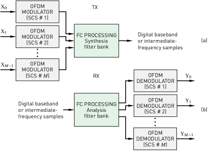
Figure 1: In fast-convolution (FC)-based filtered-OFDM, filtering is applied at subband level, which means one or multiple contiguous physical resource blocks (PRBs) with same subcarrier spacing (SCS), while utilizing normal CP-OFDM waveform for the PRBs. (a) Transmitter processing using the FC synthesis filter bank of $M$ subbands. (b) Receiver processing using FC analysis filter bank.

Initial studies on filtered OFDM were based on time-domain filtering [8, 9, 10], and later also polyphase filter-bank-based solutions have been presented [11, 12, 13, 14]. Fast-convolution-based filtered OFDM (see Fig. 1) has been presented in [15, 16, 17, 18]. Especially in [18], the flexibility, good performance, and low computational complexity of FC-based F-OFDM (FC-F-OFDM) was clearly demonstrated in the 5G-NR context. These schemes typically apply filtering in continuous manner over a frame of CP-OFDM (or zero-prefix-OFDM) symbols.

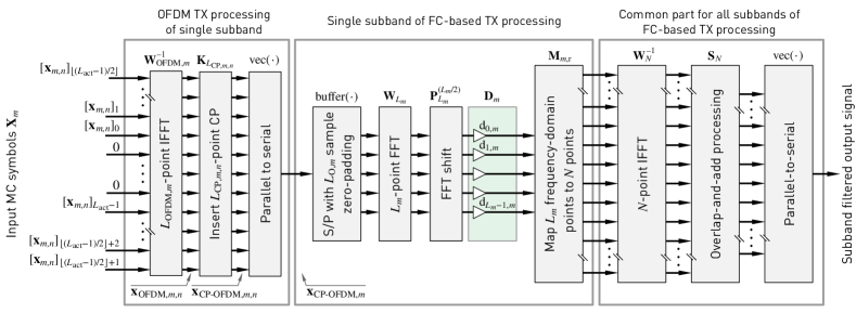
Figure 2: Block diagram for basic FC-F-OFDM transmitter processing using the OLA model.

The problematic or inconvenient aspect of the conventional time-domain filtering-based schemes is their high complexity. In [19], it was shown that the complexity of time-domain filtering based solutions in mixed-numerology case is $70$ times the complexity of CP-OFDM processing. This complexity can be reduced using classical (e.g., polyphase) filter-bank models, however, these solutions have somewhat reduced flexibility in adjusting the subband center frequencies and bandwidths. Since FC is a block-wise processing scheme with fixed block length, the position of the useful parts of the OFDM symbols vary within a frame of transmitted OFDM symbols. With the usual continuous FC-processing model as described in [15, 18], it is necessary that the CP lengths and useful symbol durations correspond to an integer number of samples at the lower sampling rate used for transmitter OFDM processing at each subband. In case of narrow-band allocations, this limits the choice of the transform lengths, significantly increasing the computational complexity. With 3GPP long-term evolution (LTE) and 5G-NR numerologies, the shortest possible transform length is $128$, while length-$16$ transform would be sufficient when a subband contains one physical-layer resource block ( physical resource block (PRB)) ($12$ subcarriers) only. This restriction applies to both time-domain filtering and FC-based solutions with continuous processing model. On the receiver side, the proposed scheme makes it possible to effectively combine cascaded inverse and forward FFT units in FC-filtered OFDM processing. Transform decomposition is used to simplify these computations, leading to significantly reduced implementation complexity in various transmission scenarios.

Building on our early work in [1], this article proposes symbol-synchronized discontinuous FC processing targeting at increased flexibility and reduced complexity of FC-F-OFDM. It is shown that the proposed processing supports more flexible parametrization of the FC engine, resulting in reduced complexity and latency with narrow subband allocations and in mini-slot transmission. Important use cases are seen, e.g., in spectrally well-contained narrow-band internet-of-things (NB IoT) transmission with one PRB allocation and in ultra-reliable low-latency communications (URLLC) for generating short transmission bursts, so-called mini-slots, to reduce the radio link latency. However, the proposed schemes can be used for wide-band allocations as well.

The proposed scheme allows to reduce the complexity in the case of (i) short transmissions (e.g. mini-slot), (ii) in multiplexing multiple relatively narrow subbands (e.g., gateway for massive machine-type communications (MTC) communications), and (iii) user equipment (UE) side transmitter (TX) processing, assuming that only one numerology is transmitted. Moreover, in case of parallelized hardware implementations, it is a benefit that each OFDM symbol can be generated and filtered independently of the others. This also minimizes the TX signal processing latency.

In this article, we develop and describe discontinuous symbol-synchronized FC-based processing techniques. The main contributions of the article can be listed as follows:

• Mathematical models for discontinuous symbol-synchronized FC-based TX and receiver (RX) processing are described. Both overlap-and-add (OLA) and overlap-and-save (OLS) variants are discussed.

• Extrapolating TX FC processing is suggested for reducing the required inverse fast Fourier transform (IFFT) size for OFDM modulation by relaxing the CP length related constraints on the IFFT size.

• Model for simplifying the IFFT computations in RX processing is proposed. The computational savings are achieved by effectively combining the computations of the IFFT of the FC module and the FFT of subband OFDM processing through transform decomposition.

• Extensive numerical results are provided, verifying the validity of the proposed models and illustrating the benefits of the proposed FC-based filtered-OFDM processing.

• Complexity evaluations are given quantifying the savings achieved using the proposed techniques.

• Discontinuous FC processing is proposed as an additional useful element in the toolbox for frequency-domain waveform processing, and it can be expected to find applications also in other areas of digital signal processing.

The remainder of this paper is organized as follows. Section II, first shortly reviews the continuous FC-based filtered-OFDM processing. Then, the proposed discontinuous TX FC-processing model is described with implementation alternatives resulting to the reduced complexity and latency in Section III for TX and in Section IV for RX. Section V presents an analysis of the computational complexity of considered alternative FC schemes. In Section VI, the performance of the discontinuous processing is analyzed in terms of uncoded bit error rate (BER) in different interference/multiplexing scenarios and channel conditions, while also numerical results for the complexity for alternative FC schemes are provided. Finally, the conclusions are drawn in Section VII.

II Continuous Fast-Convolution Processing

The block diagram for the basic continuous, symbol-nonsychronized OLA-based FC-F-OFDM TX processing for subband $m$ is shown in Fig. 2. First, the CP-OFDM signal for subband $m$ is generated by using the smallest IFFT length equal to or larger than $L_{\text{act},m}$ supporting an integer length CP. Let us denote this transform (IFFT) size by $L_{\text{OFDM},m}$. Then, low-rate CP of length $L_{\text{CP},m,n}$ is added to each of the $B_{\text{OFDM},m}$ OFDM symbols for $n=0,1,\dots,B_{\text{OFDM},m}-1$ and the signal is converted to serial format. These are all operations equivalent to basic CP-OFDM TX processing.

The actual FC processing per subband starts by partitioning the time-domain input sample stream to FC blocks, as illustrated in Fig. 2. Note that the exact number of FC processing blocks depends on the input sequence length, overlap factor, and FFT length $L_{m}$. Next, we take $L_{m}$-point FFT of each processing block and apply FFT-shift operation which essentially places the DC-carrier in the middle of each vector. Then, a frequency-domain window $\mathbf{D}_{m}$ is applied to implement the designed filter response. After frequency-domain windowing the given subband is placed at the allocated FFT bins with transition-band values possibly exceeding the nominal allocation range. The overlapping transition-band bins of adjacent subbands are added together.

The $N$-point IFFT is common part for all subbands. It converts all the low-rate frequency-division multiplexed subband signals to time domain per FC block. In addition, it provides the sampling-rate conversion by the factor of $I_{m}=N/L_{m}$. Next, OLA processing is used to concatenate the high-rate FC-blocks in order to construct the filtered time-domain representation of the transmitted signal. Alternatively, FC processing can be realized using OLS scheme. In this case, the zero padding in block partitioning is replaced by the straightforward segmentation into the overlapping blocks and the OLA after the last transform is replaced by the discarding of the overlapping output segments. More detailed description of the FC filtering process can be found, e.g., from [18, 20].

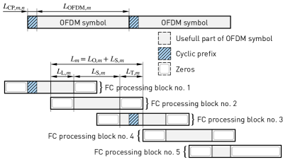
Figure 3: FC-processing block partitioning in basic continuous OLA-based FC-F-OFDM. FC blocks are not synchronized to CP-OFDM symbols. Five FC-processing blocks are needed for two OFDM symbols.

The basic continuous FC-processing flow of FC-F-OFDM transmitter for $L_{\text{OFDM},m}=L_{m}$ is illustrated in Fig. 3. The assumed overlap between processing blocks is $50\text{\,}\%$ (the overlap factor is $\lambda=0.5$). From Fig. 3 we can observe how the FC processing is continuous by collecting $L_{\text{OFDM},m}/2=L_{m}/2$ samples from the input sample stream to each FC processing block. Also, the overlap factor is constant over all FC processing blocks.

III Symbol-Synchronized Discontinuous FC-based Filtered-OFDM TX Processing

Fig. 4 illustrates the proposed discontinuous TX FC-F-OFDM processing flow for a mini-slot of two OFDM symbols ($B_{\text{OFDM},m}=2$). It can be observed that in discontinuous processing, two FC processing blocks are synchronized to each OFDM symbol, where the first FC block contains the first half of the OFDM symbol and the second FC block contains the second half of the OFDM symbol. In addition, the first FC processing block contains the low-rate CP samples. This reduces the overlap in the beginning of the first FC block, that is, the overlap factor becomes $\lambda=0.5-L_{\text{CP},m,n}/L_{m}$. Here, $L_{\text{CP},m,n}$ is the CP length of the $n$th symbol on subband $m$. In practice, this reduction is relatively small, causing only minor increase in the related distortion effects. For discontinuous processing, only four FC processing blocks are used, instead of five in the continuous processing model (see Fig. 3), resulting in reduced complexity.

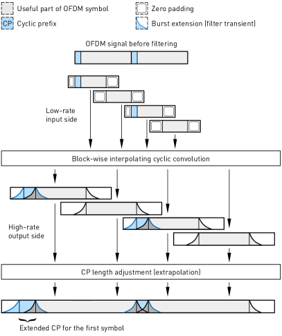
Figure 4: Discontinuous OLA-based block partitioning for FC-F-OFDM TX processing. FC processing blocks are synchronized to the OFDM symbols. Four FC-processing blocks are needed for two OFDM symbols. The FC overlap factor is dynamic: $0.5-N_{\text{CP},n}/N$ for the first block and $0.5$ for the second block of each OFDM symbol.

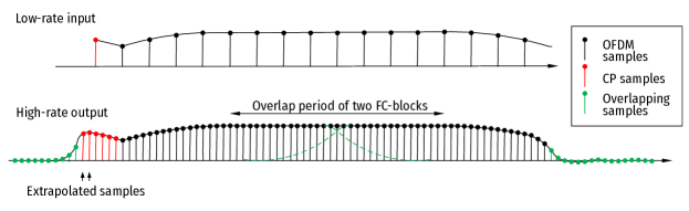
Figure 5: Discontinuous OLA processing for a single CP-OFDM symbol with $50\text{\,}\%$ FC overlap, interpolation factor of four ($I_{m}=4$), and high-rate OFDM symbol duration of $64$ samples. CP length is one sample at low rate and six samples at high rate (corresponding to one and half low-rate samples)

This scheme is particularly beneficial in cases like Fig. 4 where the FC block length is equal to the OFDM symbol duration (a common assumption in earlier studies of FC-F-OFDM) and the two halves of the basic OFDM symbol are processed in two consecutive FC blocks. Then the FC blocks are synchronized to the OFDM symbols, and the CP is also processed within the first FC block. Such discontinuous FC-based TX filter processing reduces computational complexity through dynamically adjustable overlap of consecutive CP-OFDM symbols.

Fig. 5 shows a detailed example of the sample-level interpolation and extrapolation process. The CP part is included in the leading overlap section of the first FC block of each OFDM symbol and the CP length is fine tuned in the OLA processing for consecutive OFDM symbols at high rate. The time resolution in adjusting the CP length is equal to the sampling interval at high rate (as in traditional CP-OFDM).

In generic setting, the discontinuous FC-F-OFDM process can be formulated as follows. First the CP-OFDM symbols are generated at the minimum feasible sampling rate for each subband and, if needed, the CP length is truncated to the highest integer number of low-rate samples which does not exceed the CP length of the transmitted signal. FC-based filtering (or interpolation) is applied to each CP-OFDM symbol individually to generate filtered symbols at the high (output) sampling rate. The CP-OFDM signal for a transmission slot is constructed from the generated individual symbols using the OLA principle. When combining the individual symbols, their spacing in time direction is adjusted (with the precision of the output sampling interval) to correspond to the precise CP duration.

In basic form, the proposed scheme is suitable for scenarios where the overall symbol durations of all subband signals to be transmitted have equal lengths and the symbols are synchronized. It is notable that different durations (e.g., different CP lengths) are allowed for different CP-OFDM symbol intervals within a transmission slot.

III-A CP-OFDM Processing with Variable CP Lengths

Let $L_{\text{OFDM},m}$ and $L_{\text{CP},m,n}$ be the OFDM symbol length and the CP length of the $n$th symbol, respectively, on $m$th subband for $m=0,1,\dots,M-1$, where $M$ is the number of subbands. The CP-OFDM TX processing, as illustrated in left-hand side block in Fig. 2, is formally expressed as

$$\mathbf{x}_{\text{OFDM},m,n}=\sqrt{L_{\text{OFDM},m}}\mathbf{W}_{L_{\text{OFDM},m}}^{-1}\mathbf{x}_{m,n}$$ (1a)

and

$$\mathbf{x}_{\text{CP-OFDM},m,n}=\mathbf{K}_{L_{\text{CP},m,n}}\mathbf{x}_{\text{OFDM},m,n},$$ (1b)

where $\mathbf{x}_{m,n}\in\mathbb{C}^{L_{\text{OFDM},m}\times 1}$ is the vector containing the incoming quadrature amplitude modulation (QAM) symbols on $L_{\text{act},m}$ active subcarriers, $\mathbf{W}^{-1}_{L_{\text{OFDM},m}}\in\mathbb{C}^{L_{\text{OFDM},m}\times L_{\text{OFDM},m}}$ is the inverse discrete Fourier transform (IDFT) matrix, and $\mathbf{K}_{L_{\text{CP},m,n}}\in\mathbb{Z}^{(L_{\text{OFDM},m}+L_{\text{CP},m,n})\times L_{\text{OFDM},m}}$ is the CP insertion matrix. In general, the CP length could be different for each symbol, while for 5G-NR and LTE, two CP lengths are used for normal CP configuration [21, 22] such that the first symbol of a half subframe ($0.5\text{\,}\mathrm{m}\mathrm{s}$) is longer than the others.

III-B FC-based Synthesis Filter Bank with Overlap-and-Add or Overlap-and-Save Processing

FC-based filtering carries out the processing in overlapping blocks. In the synthesis filter bank (SFB) case, the input block length of the $m$th subband is $L_{m}$ and the output block length is $N$. The overlap between the input blocks is determined by the number of overlapping input samples $L_{\text{O},m}$. The number of non-overlapping input samples is given as $L_{\text{S},m}=L_{m}-L_{\text{O},m}$ while the overlap factor is expressed using these values as

$$\lambda=L_{\text{O},m}/L_{m}=(L_{m}-L_{\text{S},m})/L_{m}.$$ (2)

The number of overlapping input samples can be further divided into leading and tailing overlapping parts as follows:

$$L_{\text{L},m}=\lceil L_{\text{O},m}/2\rceil\quad\text{and}\quad L_{\text{T},m}=\lfloor L_{\text{O},m}/2\rfloor.$$ (3)

The corresponding number of overlapping and non-overlapping output samples are determined as $N_{\text{O}}=\lambda N$ and $N_{\text{S}}=(1-\lambda)N$, respectively. Similarly, the number of overlapping output samples are divided into leading and tailing parts, $N_{\text{L}}$ and $N_{\text{T}}$, respectively.

The FC processing increases the sampling rate by the factor of

$$I_{m}=N/L_{m},$$ (4)

resulting in OFDM symbol and CP durations of $N_{\text{OFDM},m}=I_{m}L_{\text{OFDM},m}$ and $N_{\text{CP},m,n}=I_{m}L_{\text{CP},m,n}$, respectively. Here $L_{\text{OFDM},m}$ and $L_{\text{CP},m,n}$ have integer values. It is convenient, but not necessary, that $N_{\text{OFDM},m}$ and $N_{\text{CP},m,n}$ have integer values as well.

In continuous FC SFB, the filtering of the $m$th CP-OFDM subband signal for the generation of the high-rate waveform $\mathbf{w}_{m}$ can be represented as

$$\mathbf{w}_{m}=\sqrt{I_{m}}\mathbf{F}_{m}\begin{bmatrix}\mathbf{0}_{S_{\text{L},m}\times 1}\\ \mathbf{x}_{\text{CP-OFDM},m}\\ \mathbf{0}_{S_{\text{L},m}\times 1}\end{bmatrix},$$ (5a)

where $$\mathbf{F}_{m}$$ is the block diagonal transform matrix of the form

$$\mathbf{F}_{m} =\operatorname{diag}\left(\mathbf{F}_{m,0}(\varphi_{m,0}),\mathbf{F}_{m,1}(\varphi_{m,1}),\dots,\mathbf{F}_{m,R_{m}-1}(\varphi_{m,R_{m}-1})\right)$$ (5b)

with $R_{m}$ overlapping blocks $\mathbf{F}_{m,r}(\varphi_{m,r})\in\mathbb{C}^{N\times L_{m}}$ for $r=0,1,\dots,R_{m}-1$. Here, $\mathbf{x}_{\text{CP-OFDM},m}$ is the column vector formed by concatenating the $\mathbf{x}_{\text{CP-OFDM},m,n}$ for $n=0,1,\dots,B_{\text{OFDM},m}-1$. The zero-padding before and after the CP-OFDM symbols is typically selected to be $S_{\text{L},m}=L_{m}-L_{\text{S},m}$. The overall high-rate waveform to be transmitted is then obtained by combining all the subband waveforms as follows:

$$\mathbf{x}_{\text{FC-F-OFDM}}=\sum_{m=0}^{M-1}\mathbf{w}_{m}.$$ (6)

The multirate version of the FC SFB can be represented either using the OLA block processing by decomposing the $\mathbf{F}_{m,r}(\varphi_{m,r})$’s as the following matrix

$$\mathbf{F}^{\text{(OLA)}}_{m,r}(\varphi_{m,r})=\mathbf{W}^{-1}_{N}\mathbf{M}_{m}(\varphi_{m,r})\mathbf{D}_{m}\mathbf{P}^{(L_{m}/2)}_{L_{m}}\mathbf{W}_{L_{m}}\mathbf{A}_{m,r}$$ (7a)

or OLS block processing when the $$\mathbf{F}_{m,r}(\varphi_{m,r})$$’s are decomposed as

$$\mathbf{F}^{\text{(OLS)}}_{m,r}(\varphi_{m,r})=\mathbf{S}_{m,r}\mathbf{W}^{-1}_{N}\mathbf{M}_{m}(\varphi_{m,r})\mathbf{D}_{m}\mathbf{P}^{(L_{m}/2)}_{L_{m}}\mathbf{W}_{L_{m}}.$$ (7b)

Here, $\mathbf{W}_{L_{m}}\in\mathbb{C}^{L_{m}\times L_{m}}$ and $\mathbf{W}_{N}^{-1}\in\mathbb{C}^{N\times N}$ are discrete Fourier transform (DFT) and IDFT matrices, respectively. The DFT shift matrix $\mathbf{P}^{(L_{m}/2)}_{L_{m}}\in\mathbb{N}^{L_{m}\times L_{m}}$ is circulant permutation matrix expressed as

$$\mathbf{P}^{(L_{m}/2)}_{L_{m}}=\begin{bmatrix}\mathbf{0}_{{\lfloor L_{m}/2\rfloor}\times{\lceil L_{m}/2\rceil}}&\mathbf{I}_{\lfloor L_{m}/2\rfloor}\\ \mathbf{I}_{\lceil L_{m}/2\rceil}&\mathbf{0}_{{\lceil L_{m}/2\rceil}\times{\lfloor L_{m}/2\rfloor}}\end{bmatrix}$$ (8)

while $\mathbf{D}_{m}\in\mathbb{R}^{L_{m}\times L_{m}}$ is diagonal matrix with diagonal elements being the weights of the subband $m$. The frequency-domain mapping matrix $\mathbf{M}_{m}(\varphi_{m,r})\in\mathbb{N}^{N\times L_{m}}$ maps $L_{m}$ frequency-domain bins of the input signal to frequency-domain bins of the output signal as follows:

$$[\mathbf{M}_{m}(\varphi_{m,r})]_{q,p}=\begin{cases}\varphi_{m,r},&\text{if $\Xi(p)=q$}\\ 0,&\text{otherwise}\end{cases}$$ (9a)

with

$$\Xi(p)=(c_{m}-\lceil{{L_{m}}/{2}}\rceil+p-1\bmod N)+1,$$ (9b)

where $$c_{m} m$$ is the center bin of the subband . The phase rotation needed to maintain the phase continuity between the consecutive overlapping processing blocks is given as

$$\varphi_{m,r}=\exp({\mathop{\mspace{1.0mu}\mathrm{j}\mspace{0.5mu}}\nolimits}2\pi rc_{m}L_{\text{S},m}/L_{m}).$$ (9c)

For further details, see [18].

For OLA processing, the time-domain analysis window matrix $\mathbf{A}_{m,r}\in\mathbb{N}^{L_{m}\times L_{m}}$ is a diagonal weighting matrix as given by

$$\mathbf{A}_{m,r}=\operatorname{diag}\left(\mathbf{a}_{m,r}\right)\quad\text{with}\quad\mathbf{a}_{m,r}=\begin{bmatrix}\mathbf{0}_{L_{\text{L},m}\times 1}\\ \mathbf{1}_{L_{\text{S},m}\times 1}\\ \mathbf{0}_{L_{\text{T},m}\times 1}\end{bmatrix}.$$ (10a)

For OLS processing, the time-domain synthesis window matrix $$\mathbf{S}_{m,r}\in\mathbb{N}^{N\times N}$$ is given by

$$\mathbf{S}_{m,r}=\operatorname{diag}\left(\mathbf{s}_{m,r}\right)\quad\text{with}\quad\mathbf{s}_{m,r}=\begin{bmatrix}\mathbf{0}_{N_{\text{L}}\times 1}\\ \mathbf{1}_{N_{\text{S}}\times 1}\\ \mathbf{0}_{N_{\text{T}}\times 1}\end{bmatrix}.$$ (10b)

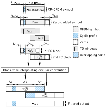
Figure 6: Overlap-and-add (OLA)-based block processing of one CP-OFDM symbol using two FC-processing blocks.

III-C Symbol-Synchronized TX FC Processing for One CP-OFDM Symbol

Fig. 6 illustrates the OLA-based FC processing of one CP-OFDM symbol in two processing blocks corresponding to overlap factor of $\lambda=0.5$. Here, it is assumed that the OFDM modulation IFFT lengths and the FC-processing short transform (FFT) lengths are the same, that is, $L_{\text{OFDM},m}=L_{m}$ for $m=0,1,\dots,M-1$.

In symbol-synchronized processing, the incoming symbol is first zero padded in the beginning and the end by $S_{\text{L},m,n}=L_{{\text{L}},m}-L_{\text{CP},m,n}$ and $L_{\text{T},m}$ zeros, respectively, to form a zero-padded symbol ${\mathbf{z}}_{m,n}$ of length $3/2L_{m}$ as follows

$${\mathbf{z}}_{m,n}=\begin{bmatrix}\mathbf{0}_{S_{\text{L},m,n}\times(L_{\text{OFDM},m}+L_{\text{CP},m,n})}\\ \mathbf{I}_{L_{\text{OFDM},m}+L_{\text{CP},m,n}}\\ \mathbf{0}_{L_{\text{T},m}\times(L_{\text{OFDM},m}+L_{\text{CP},m,n})}\\ \end{bmatrix}\mathbf{x}_{\text{CP-OFDM},m,n}.$$ (11)

Now, $\mathbf{F}_{m,r}(\varphi_{m,r})$’s for $r=0,1$ essentially process (filter and possibly interpolate) two overlapping segments of length $L_{m}$ from the zero-padded symbol. Let us denote these segments by ${\mathbf{z}}^{(r)}_{m,n}\in\mathbb{C}^{L_{m}\times 1}$ for $r=0,1$ and the samples belonging to these processing segments are given by

$${\mathbf{z}}^{(r)}_{m,n}=(\mathbf{R}_{L_{m}}^{(r)})^{\mathchoice{\raisebox{0.0pt}{$\displaystyle\intercal$}}{\raisebox{0.0pt}{$\textstyle\intercal$}}{\raisebox{0.0pt}{$\scriptstyle\intercal$}}{\raisebox{0.0pt}{$\scriptscriptstyle\intercal$}}}{\mathbf{z}}_{m,n}$$ (12a)

for $$r=0,1$$ where

$$\mathbf{R}_{L_{m}}^{(0)}=\begin{bmatrix}\mathbf{I}_{L_{m}}\\ \mathbf{0}_{L_{m}/2\times L_{m}}\end{bmatrix}\qquad\text{and}\qquad\mathbf{R}_{L_{m}}^{(1)}=\begin{bmatrix}\mathbf{0}_{L_{m}/2\times L_{m}}\\ \mathbf{I}_{L_{m}}\end{bmatrix}.$$ (12b)

The effective overlap factor for the first processing block is reduced to $0.5-L_{\text{CP},m,n}/L_{m}$ due to inclusion of CP and, therefore, the first time-domain analysis window has to be redefined to

$$\mathbf{a}_{m,0}=\begin{bmatrix}\mathbf{0}_{S_{\text{L},m,n}\times 1}\\ \mathbf{1}_{L_{\text{S},m}+L_{\text{CP},m,n}\times 1}\\ \mathbf{0}_{L_{\text{T},m}\times 1}\end{bmatrix}$$ (13)

as well. Let $\mathbf{w}_{m,n}^{(r)}\in\mathbb{C}^{N\times 1}$ for $r=0,1$ denote the product of the processing blocks by the transform matrices as expressed by

$$\mathbf{w}_{m,n}^{(r)}=\mathbf{F}_{m,r}(\varphi_{m,r}\theta_{n}){\mathbf{z}}^{(r)}_{m,n}$$ (14a)

for $$r=0,1$$. Here, an additional phase rotation as given by

$$\theta_{n}=\exp({\mathop{\mspace{1.0mu}\mathrm{j}\mspace{0.5mu}}\nolimits}2\pi c_{m}\varphi_{n})$$ (14b)

with

$$\varphi_{n}=\frac{1}{N}\sum_{q=1}^{n}N_{\text{CP},m,q},$$ (14c)

is included to compensate the truncation of the CP length to interger samples on the low-rate side.

The filtered high-rate subband waveform of length $3/2N$ corresponding the $n$th symbol on the $m$th subband can finally obtained be combining these filtered blocks as

$$\mathbf{w}_{m,n}=\sum_{r=0,1}\mathbf{R}^{(r)}_{N}{\mathbf{w}}_{m,n}^{(r)}$$ (15a)

where

$$\mathbf{R}_{N}^{(0)}=\begin{bmatrix}\mathbf{I}_{N}\\ \mathbf{0}_{N/2\times N}\end{bmatrix}\quad\text{and}\quad\mathbf{R}_{N}^{(1)}=\begin{bmatrix}\mathbf{0}_{N/2\times N}\\ \mathbf{I}_{N}\end{bmatrix}.$$ (15b)

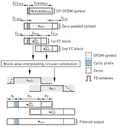
Figure 7: Overlap-and-save (OSA)-based block processing of one CP-OFDM symbol using two FC-processing blocks.

Alternative to OLA scheme, the above processing can also be carried out following the OLS approach as illustrated in Fig. 7. The basic difference is that now the time-domain windowing is realized after the convolution and only one of the filtered blocks is non-zero in the overlapping regions. The abrupt truncation of output waveform at the edges of the filtered symbol can be avoided by smoothly tapering the raising edge of the first time-domain synthesis window $\mathbf{s}_{m,0}$ and the falling edge of the second time-domain window $\mathbf{s}_{m,1}$, as illustrated using the dashed line in Fig. 7. Discontinuities in the output waveform give raise to a high spectral leakage and, therefore, the OLA scheme is preferable on the TX side in general.

III-D Symbol-Synchronized TX FC Processing for Multiple Symbols

In the case of multiple OFDM symbols, the high-rate filtered symbols are combined with symbol-wise OLA processing as follows

$$\mathbf{w}_{m}=\sum_{n=0}^{B_{\text{OFDM},m}-1}\boldsymbol{\Gamma}_{\sigma_{n}}\mathbf{w}_{m,n}$$ (16a)

with

$$\sigma_{n}=nN_{\text{OFDM},m}+\sum_{q=1}^{n}N_{\text{CP},m,q}$$ (16b)

being the starting index of the $$n \mathbf{w}_{m,n} 3/2N_{\text{OFDM},m} \mathbf{w}_{m} Q 3/2N$$th filtered block of length in as illustrated in Fig. 8. Here, -by- matrix

$$\boldsymbol{\Gamma}_{p}=\begin{bmatrix}\mathbf{0}_{p\times 3/2N}\\ \mathbf{I}_{3/2N}\\ \mathbf{0}_{(Q-3/2N-p)\times 3/2N}\end{bmatrix}$$ (16c)

with

$$Q=N_{\text{L},m}+N_{\text{T},m}+B_{\text{OFDM},m}N_{\text{OFDM},m}+\sum_{n=1}^{B_{\text{OFDM},m}-1}N_{\text{CP},m,n}$$ (16d)

aligns the filtered symbols to their desired time-domain locations at the high-rate output sequence.

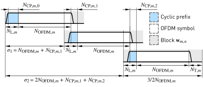
Figure 8: Symbol-wise overlap-and-add processing for concatenating the filtered CP-OFDM symbols.

III-E CP Extrapolation by TX FC Processing

Suppose that $L_{\text{OFDM},m}$ is chosen such that the CP length on the low-rate side is not an integer, that is, $L_{\text{OFDM},m}<128$ for 5G-NR and LTE numerologies. In this case, CP length can be rounded to next smaller integer as given by

$$L_{\text{CP},m,n}=\lfloor N_{\text{CP},m,n}/I_{m}\rfloor$$ (17)

and the FC-based filtering with the accompanying symbol-wise overlap-and-add processing as given by (16) inherently extrapolates at the high-rate side $N_{\text{CP},m,n}-N/L_{m}L_{\text{CP},m,n}$ samples corresponding to fractional part of the low-rate CP.

As an example, in the $10\text{\,}\mathrm{M}\mathrm{H}\mathrm{z}$ 5G-NR or LTE case with $15\text{\,}\mathrm{k}\mathrm{H}\mathrm{z}$ SCS and normal CP length, the output sampling rate is $f_{\text{s,out}}=$15.36\text{\,}\mathrm{M}\mathrm{H}\mathrm{z}$$, the useful OFDM symbol duration is $N_{\text{OFDM},m}=1024$ high-rate samples, and the CP length is $N_{\text{CP},m,n}=80$ high-rate samples for the first symbol (for $n\bmod 7=0$) of each slot of $7$ symbols, and $N_{\text{CP},m,n}=72$ samples for the others (for $n\bmod 7\neq 0$). Then in the continuous processing model, the smallest possible OFDM IFFT length is $L_{\text{OFDM},m}=128$, corresponding to $f_{\text{s,in}}=$1.92\text{\,}\mathrm{M}\mathrm{H}\mathrm{z}$$ input sampling rate, and the CP lengths are $L_{\text{CP},m,n}=10$ and $L_{\text{CP},m,n}=9$ low-rate samples for the first and other symbols, respectively. However, using the discontinuous FC processing model with narrow subband allocations, like $12$, $24$, or $48$ subcarriers, the OFDM IFFT length $L_{\text{OFDM},m}$ can be reduced to $16$, $32$, or $64$, respectively. These transform lengths correspond at the low-rate side to CP lengths $L_{\text{CP},m,n}$ of $1.25$, $2.5$, and $5.0$ for the first symbol or $1.125$, $2.25$, and $4.5$ for the others. The same transform (IFFT) lengths are used for the subband OFDM signal generation. One important case is NB IoT using $180\text{\,}\mathrm{k}\mathrm{H}\mathrm{z}$ transmission bandwidth corresponding to a single PRB ($12$ SCs) and needs IFFT length of $128$ and sampling rate of $1.92\text{\,}\mathrm{M}\mathrm{H}\mathrm{z}$ in traditional implementation. Discontinuous processing allows to generate the signal by using the FFT size of $16$ for the OFDM symbol generation and FC processing at the sampling rate of $240\text{\,}\mathrm{k}\mathrm{H}\mathrm{z}$.

IV Symbol-Synchronized Discontinous FC-based Filtered-OFDM RX Processing

As for the TX side, the basic continuous FC-processing flow of FC-F-OFDM RX requires five FC-processing blocks in order to process two CP-OFDM symbols. In this case, the CPs are discarded after the FC filtering as part of normal RX CP-OFDM reception. With continuous processing, the FC-processing chain needs to wait for varying number of samples belonging to the second OFDM symbol before it can start processing the third FC-processing block in order to obtain final samples in the output for the first OFDM symbol. In discontinuous processing, as seen in Fig. 9, the RX waits only for the samples belonging to the first OFDM symbol and desired amount of overlapping samples from the beginning of the second symbol, after which it can start processing the second FC processing block, providing at the output the last filtered samples of the first OFDM symbol.

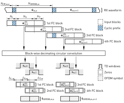
Figure 9: Discontinuous OLS processing for FC-F-OFDM receiver with overlap factor of $\lambda=0.5$. FC processing blocks are synchronized to the OFDM symbols. Four FC-processing blocks are needed for two OFDM symbols.

In the case of maximal timing-adjustment flexibility, the number of samples collected from the following CP-OFDM symbol time corresponds to the number of overlapping samples at the end of FC processing block. In addition, in discontinuous processing, two first FC processing blocks can be processed independently from the two following FC processing blocks, as they represent different OFDM symbols. In continuous processing, two OFDM symbols are linked through common samples in the third FC processing block.

Because the content (FC block contains first or second half of OFDM symbol) and processing of even and odd FC processing blocks remain constant over the whole RX signal, we can process even and odd blocks separately from each other. This allows for an implementation where even and odd FC processing blocks are processed in parallel FC processing chains, allowing to minimize the latency of the RX implementation.

In the RX case, the transform matrices for FC processing with OLA and OLS schemes are given as

$$\mathbf{G}^{\text{(OLA)}}_{m,r}(\varphi_{m,r}) =\mathbf{W}^{-1}_{L_{m}}\mathbf{P}^{(-L_{m}/2)}_{L_{m}}\mathbf{D}_{m}\mathbf{M}_{m,r}(\varphi_{m,r})^{\mathchoice{\raisebox{0.0pt}{$\displaystyle\intercal$}}{\raisebox{0.0pt}{$\textstyle\intercal$}}{\raisebox{0.0pt}{$\scriptstyle\intercal$}}{\raisebox{0.0pt}{$\scriptscriptstyle\intercal$}}}\mathbf{W}_{N}\mathbf{{A}}_{m,r}$$

$$=\operatorname{conj}(\mathbf{F}^{\text{(OLS)}}_{m,r}(\varphi_{m,r}))^{\mathchoice{\raisebox{0.0pt}{$\displaystyle\intercal$}}{\raisebox{0.0pt}{$\textstyle\intercal$}}{\raisebox{0.0pt}{$\scriptstyle\intercal$}}{\raisebox{0.0pt}{$\scriptscriptstyle\intercal$}}}$$ (18a)

and

$$\mathbf{G}^{\text{(OLS)}}_{m,r}(\varphi_{m,r}) =\mathbf{{S}}_{m,r}\mathbf{W}^{-1}_{L_{m}}\mathbf{P}^{(-L_{m}/2)}_{L_{m}}\mathbf{D}_{m}\mathbf{M}_{m,r}(\varphi_{m,r})^{\mathchoice{\raisebox{0.0pt}{$\displaystyle\intercal$}}{\raisebox{0.0pt}{$\textstyle\intercal$}}{\raisebox{0.0pt}{$\scriptstyle\intercal$}}{\raisebox{0.0pt}{$\scriptscriptstyle\intercal$}}}\mathbf{W}_{N}$$

$$=\operatorname{conj}(\mathbf{F}^{\text{(OLA)}}_{m,r}(\varphi_{m,r}))^{\mathchoice{\raisebox{0.0pt}{$\displaystyle\intercal$}}{\raisebox{0.0pt}{$\textstyle\intercal$}}{\raisebox{0.0pt}{$\scriptstyle\intercal$}}{\raisebox{0.0pt}{$\scriptscriptstyle\intercal$}}},$$ (18b)

respectively, while the time-domain analysis and synthesis window matrices are now given as

$$\mathbf{A}_{m,r}=\operatorname{diag}\left(\begin{bmatrix}\mathbf{0}_{N_{\text{L}}\times 1}\\ \mathbf{1}_{N_{\text{S}}\times 1}\\ \mathbf{0}_{N_{\text{T}}\times 1}\end{bmatrix}\right)\quad\text{and}\quad\mathbf{S}_{m,r}=\operatorname{diag}\left(\begin{bmatrix}\mathbf{0}_{L_{\text{L},m}\times 1}\\ \mathbf{1}_{L_{\text{S},m}\times 1}\\ \mathbf{0}_{L_{\text{T},m}\times 1}\end{bmatrix}\right),$$ (19a)

respectively.

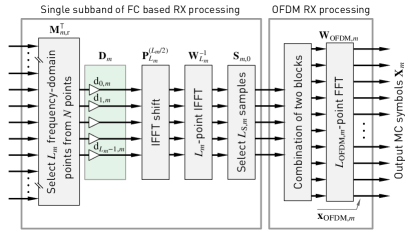
Figure 10: Block diagram for discontinuous FC-F-OFDM receiver processing using the overlap-save model.

The RX side discontinuous FC processing starts by segmenting the received high-rate waveform $\mathbf{\hat{x}}_{\text{FC-F-OFDM}}$ into the blocks of length $3/2N$ as

$$\mathbf{\hat{w}}_{m,n}=\sum_{n=0}^{B_{\text{OFDM},m}-1}\boldsymbol{\Gamma}_{\sigma_{n}}^{\mathchoice{\raisebox{0.0pt}{$\displaystyle\intercal$}}{\raisebox{0.0pt}{$\textstyle\intercal$}}{\raisebox{0.0pt}{$\scriptstyle\intercal$}}{\raisebox{0.0pt}{$\scriptscriptstyle\intercal$}}}\mathbf{\hat{x}}_{\text{FC-F-OFDM}}.$$ (20a)

Here, it is assumed for simplicity that the length of the received waveform is $$Q I_{m}S_{\text{L},m,n} \mathbf{\hat{w}}_{m,n} N$$ as given by (16d) and that the waveform is synchronized such that it contains samples before the first data symbol. The high-rate symbols are further divided into the overlapping blocks of length as

$$\mathbf{\hat{w}}_{m,n}^{(r)}=(\mathbf{R}_{N}^{(r)})^{\mathchoice{\raisebox{0.0pt}{$\displaystyle\intercal$}}{\raisebox{0.0pt}{$\textstyle\intercal$}}{\raisebox{0.0pt}{$\scriptstyle\intercal$}}{\raisebox{0.0pt}{$\scriptscriptstyle\intercal$}}}\mathbf{\hat{w}}_{m,n},$$ (20b)

for $$r=0,1 \mathbf{G}_{m,r}(\varphi_{m,r})$$. These blocks are processed by ’s as

$$\mathbf{\hat{z}}_{m,n}^{(r)}=\mathbf{G}_{m,r}(\varphi_{m,r}){\mathbf{\hat{w}}}^{(r)}_{m,n}$$ (20c)

for $$r=0,1 n m$$ to obtain filtered low-rate FC blocks corresponding to first and second half of the th symbol on subband . Finally, the filtered blocks are concatenated and the extensions are removed as

$$\mathbf{\hat{x}}_{\text{OFDM},m,n}=\begin{bmatrix}\mathbf{0}_{S_{\text{T},m,n}\times L_{\text{OFDM},m}}\\ \mathbf{I}_{L_{\text{OFDM},m}}\\ \mathbf{0}_{S_{\text{T},m}\times L_{\text{OFDM},m}}\end{bmatrix}^{\mathchoice{\raisebox{0.0pt}{$\displaystyle\intercal$}}{\raisebox{0.0pt}{$\textstyle\intercal$}}{\raisebox{0.0pt}{$\scriptstyle\intercal$}}{\raisebox{0.0pt}{$\scriptscriptstyle\intercal$}}}\sum_{r=0,1}\mathbf{R}^{(r)}_{L_{m}}{\mathbf{\hat{z}}}_{m,n}^{(r)},$$ (20d)

and the resulting low-rate OFDM symbol is converted back to frequency domain as a part of the OFDM demodulation process as follows:

$$\mathbf{\hat{x}}_{m,n}=\frac{1}{\sqrt{L_{\text{OFDM},m}}}\mathbf{W}_{L_{\text{OFDM},m}}\mathbf{\hat{x}}_{\text{OFDM},m,n}.$$ (20e)

Alternatively, the concatenation and the removal of the extensions can be combined in

$$\mathbf{\hat{x}}_{\text{OFDM},m,n}=\mathbf{P}_{L_{m}}^{(L_{m}/4)}\mathbf{\hat{z}}_{m,n}^{(0)}+\mathbf{P}_{L_{m}}^{(-L_{m}/4)}\mathbf{\hat{z}}_{m,n}^{(1)},$$ (20f)

where

$$\mathbf{P}_{L_{m}}^{(L_{m}/4)} =\begin{bmatrix}\begin{matrix}\mathbf{0}_{L_{m}/2\times L_{m}/4}&\mathbf{I}_{L_{m}/2}&\mathbf{0}_{L_{m}/2\times L_{m}/4}\end{matrix}\\ \mathbf{0}_{L_{m}/2\times L_{m}}\end{bmatrix}$$ (20g)

and

$$\mathbf{P}_{L_{m}}^{(-L_{m}/4)} =\begin{bmatrix}\mathbf{0}_{L_{m}/2\times L_{m}}\\ \begin{matrix}\mathbf{0}_{L_{m}/2\times L_{m}/4}&\mathbf{I}_{L_{m}/2}&\mathbf{0}_{L_{m}/2\times L_{m}/4}\end{matrix}\end{bmatrix}.$$ (20h)

This latter form is beneficial when finding the simplified implementations for the discontinuous RX processing, as described in next section.

V Implementation Complexity

The FC processing complexity can be divided into high-rate side complexity, $C_{\text{high-rate}}$, corresponding to long FC-processing transform and low-rate (or subband-wise) complexity, $C_{\text{low-rate},m}$, corresponding to short FC-processing transform, frequency-domain windowing, and OFDM (de)modulation transform. Let us denote the FC RX processing long transform (FFT) and short transform (IFFT) complexities given in terms of number of real multiplications by $\mu(N)$ and $\mu(L_{m})$, respectively, and OFDM transform (FFT) complexity by $\mu(L_{\text{OFDM},m})$.

The number of real multiplications per received data symbol can now be evaluated as

$$C_{\text{mult}}=\frac{C_{\text{high-rate}}+\sum_{m=0}^{M-1}C_{\text{low-rate},m}}{\sum_{m=0}^{M-1}L_{\text{act},m}},$$ (21a)

where the high-rate and low-rate complexities per subband are defined, respectively, as

$$C_{\text{high-rate}} =\alpha\mu(N)$$ (21b)

and

$$C_{\text{low-rate},m} =\alpha\beta\mu(L_{m})+6\alpha N_{\text{tb},m}+\mu(L_{\text{OFDM},m}).$$ (21c)

Here, $N_{\text{tb},m}$ is the number of transition-band bins per transition band, $\alpha=2$ is the number of FC blocks per OFDM symbol, and $\beta\leq 1$ is the implementation related factor as described in the next subsection. Factor $6$ in (21c) is due to fact that two transition bands are needed for each subband and one complex non-trivial transition-band bin requires three real multiplications in general.

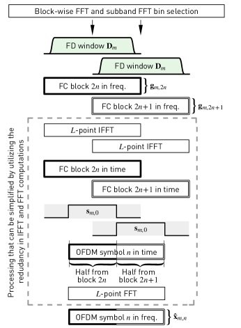
Figure 11: Discontinuous processing for one output OFDM symbol. Dashed block represents the processing that can be simplified by sharing the IFFT computations.

For 5G-NR and LTE numerologies, the minimum allocation size is one PRB corresponding to $12$ subcarriers. In this case, the minimum usable FFT size for continuous processing is $L_{\text{OFDM},m}=L_{m}=128$ whereas for discontinuous processing, FFT of size $L_{\text{OFDM},m}=L_{m}=16$ can be used. Assuming that an efficient implementation (using split-radix algorithm) requires

$$\mu(L)=L\log_{2}(L)-3L+4$$ (22)

real multiplications for transform of size $L$, each transform of size $128$ requires $\mu(128)=516$ real multiplications and each transform of size $16$ requires $\mu(16)=20$ real multiplications. These complexities are evaluated according to scheme requiring three real multiplications per complex multiplication as described in [23].

V-A Simplified Implementation

The basic idea for joint processing of the IFFTs of the FC-based filter and the FFT of OFDM receiver is shown in Fig. 11. This structure is made possible by the symbol-synchronized discontinuous RX processing scheme.

Here, it is assumed that the length of the subband-wise OFDM symbol and the size of the IFFT used in discontinuous RX FC processing are the same $L\equiv L_{\text{OFDM},m}=L_{m}$. $L$ is selected such that it contains all active SCs per subband and transition-band bins used in the frequency-domain windowing performed in the “Block-wise FFT, subband FFT bin selection and weighting” block.

For simplicity, we denote the time-domain synthesis window matrix $\mathbf{S}_{m,r}$ by $\mathbf{S}$. Now, the processing of the $n$th symbol from the frequency-domain FC output blocks $\mathbf{g}_{m,2n}$ and $\mathbf{g}_{m,2n+1}$ can be written as

$$\mathbf{\hat{x}}_{m,n} =\mathbf{W}_{L}\begin{bmatrix}\mathbf{P}_{L}^{(L/4)}\mathbf{S}\mathbf{W}_{L}^{-1}\mathbf{g}_{m,2n}+\mathbf{P}_{L}^{(-L/4)}\mathbf{S}\mathbf{W}_{L}^{-1}\mathbf{g}_{m,2n+1}\end{bmatrix}.$$ (23)

Here, $\mathbf{P}_{L}^{(L/4)}$ and $\mathbf{P}_{L}^{(-L/4)}$ are given by (20g) and (20h), respectively. Alternatively, (23) can be represented as

$$\mathbf{\hat{x}}_{m,n}=\mathbf{F}_{0}\mathbf{g}_{m,2n}+\mathbf{F}_{1}\mathbf{g}_{m,2n+1},$$ (24a)

where

$$\mathbf{F}_{0}=\mathbf{W}_{L}\mathbf{P}_{L}^{(L/4)}\mathbf{S}\mathbf{W}_{L}^{-1}\quad\text{and}\quad\mathbf{F}_{1}=\mathbf{W}_{L}\mathbf{P}_{L}^{(-L/4)}\mathbf{S}\mathbf{W}_{L}^{-1}$$ (24b)

are circular convolution matrices.

After some manipulations (23) can be reformulated as

$$\mathbf{\hat{x}}_{m,n}=\boldsymbol{\Omega}_{-L/4}[\mathbf{F}(\mathbf{g}_{m,2n}-\boldsymbol{\Omega}_{L/2}\mathbf{g}_{m,2n+1})+\boldsymbol{\Omega}_{L/2}\mathbf{g}_{m,2n+1}],$$ (25a)

where

$$\mathbf{F}=\boldsymbol{\Omega}_{L/4}\mathbf{C}\boldsymbol{\Omega}_{-L/4}$$ (25b)

with

$$\mathbf{C}=\mathbf{W}_{L}\mathbf{\hat{S}}\mathbf{W}_{L}^{-1}$$ (25c)

and

$$\boldsymbol{\Omega}_{\phi}=\operatorname{diag}\left(\begin{bmatrix}W_{L}^{0}&W_{L}^{\phi}&\cdots&W_{L}^{\phi(L-1)}\end{bmatrix}^{\mathchoice{\raisebox{0.0pt}{$\displaystyle\intercal$}}{\raisebox{0.0pt}{$\textstyle\intercal$}}{\raisebox{0.0pt}{$\scriptstyle\intercal$}}{\raisebox{0.0pt}{$\scriptscriptstyle\intercal$}}}\right)$$ (25d)

with $$W_{L}=\exp(-{\mathop{\mspace{1.0mu}\mathrm{j}\mspace{0.5mu}}\nolimits}{2}\pi/L) \mathbf{\hat{S}}\in\mathbb{Z}^{L\times L}$$. Here, as given by

$$\mathbf{\hat{S}}=\mathbf{P}_{L}^{(L/4)}\mathbf{S}\mathbf{P}_{L}^{(-L/4)}$$ (25e)

is the time-domain synthesis window matrix circularly left and up shifted by $L/4$ samples.

The above formulation relies on rotating the $\mathbf{g}_{m,2n+1}$ and the corresponding window by $L/2$ samples. In this case, $\mathbf{F}_{0}$ and $\mathbf{F}_{1}$ form a lowpass-highpass filter pair essentially meaning that $\mathbf{F}_{0}\mathbf{F}_{1}=\mathbf{I}_{L}$. The low-rate complexity of (25) per OFDM symbol is one IFFT and one FFT of length $L$ as depicted in Fig. 12. The direct approach, as illustrated in Fig. 11, requires two IFFTs and one FFT of length $L$, that is, the saving in number of real multiplications for this simplified processing is $33.3\text{\,}\%$. In (21), $\beta=1/2$ gives the complexity of the simplified processing whereas $\beta=1$ gives the complexity of the direct approach. The half-band filtering provided by (25c) can be further decomposed into smaller transforms to achieve some savings in implementation, however, these decompositions are beyond the scope of this paper.

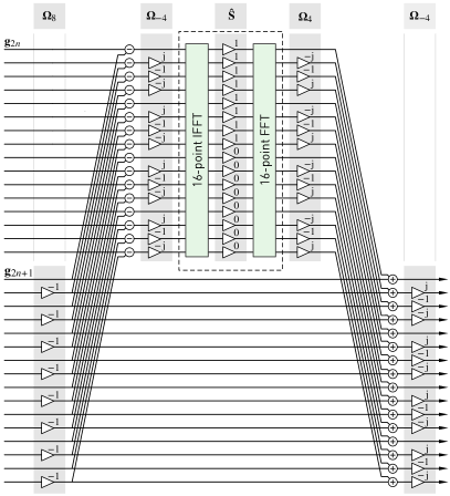
Figure 12: Simplified discontinuous processing for $L=16$ as described by (25). The dashed region can be further simplified by decomposing transforms into smaller transforms.

VI Numerical results

In this section, we will analyze the performance of the discontinuous FC processing in terms of uncoded BER in different interference and channel conditions, and also show complexity comparison between continuous and discontinuous FC processing. Here we assume the overlap factor of $\lambda=0.5$. Continuous FC processing with the overlap of $\lambda=0.25$ marginally degrades the spectral containment and error vector magnitude (EVM) performance compared to the overlap of $\lambda=0.5$ with the benefit of somewhat lower implementation complexity.

TABLE I: Narrow-band transmission scenarios and filtering configurations

Channel model	Additive white Gaussian noise (AWGN)			Tapped-delay line (TDL)-C with $300\text{\,}\mathrm{n}\mathrm{s}$ and $1000\text{\,}\mathrm{n}\mathrm{s}$ root mean squared (RMS) channel delay spread
Synchronicity	Quasi-synchronous: No timing offset and no frequency offset between different uplink signals			Asynchronous: Timing offset of 256 samples ($L_{\text{OFDM},m}/4$) between the target subband for BER evaluation and adjacent subbands on both sides
Allocated subband width	$1\text{\,}\mathrm{\text{PRB}}$, 12 single-carriers: 8 active SCs and 4-SC guardbands between adjacent active subbands			$4\text{\,}\mathrm{\text{PRBs}}$, 48 SCs: 44 active SCs and 4-SC guardband between adjacent active subbands
Filtering configuration	1) No filtering on TX and RX sides	2) No TX filtering, RX filtering with continuous FC model with $L_{\text{RX}}=128$	3) Continuous TX filtering, continuous RX filtering, $L_{\text{TX}}=L_{\text{RX}}=128$
	4) Discontinuous TX filtering, continuous RX filtering, $L_{\text{TX}}=L_{\text{RX}}=128$	5) Discontinuous TX filtering, continuous RX filtering, $L_{\text{TX}}=16$ with $1\text{\,}\mathrm{\text{PRB}}$, $L_{\text{TX}}=64$ with $4\text{\,}\mathrm{\text{PRBs}}$, and $L_{\text{RX}}=128$	6) Discontinuous TX and RX filtering, $L_{\text{TX}}=16$ with $1\text{\,}\mathrm{\text{PRB}}$, $L_{\text{TX}}=64$ with $4\text{\,}\mathrm{\text{PRBs}}$, and $L_{\text{RX}}=128$

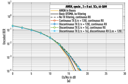
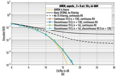
Figure 13: Simulation results with AWGN channel and 64-QAM modulation. (a) Quasi-synchronous cases and (b) asynchronous cases (quarter-symbol timing offset). Single PRB allocated for each of the three subbands (12 SCSs, 8 active SCs, and 4 SCs for guardband).

VI-A Bit-Error Rate Performance in Narrow-band Allocations

Figs. 13–17 compare the simulated uncoded BER performance of different CP-OFDM configurations, with or without subband filtering in $10\text{\,}\mathrm{M}\mathrm{H}\mathrm{z}$ 5G-NR uplink scenario, with high-rate IFFT size of $N=1024$ and SCS of $15\text{\,}\mathrm{k}\mathrm{H}\mathrm{z}$. Table I shows details of the considered scenarios and filtering configurations. The used channel models are additive white Gaussian noise (AWGN) and tapped-delay line (TDL)-C, which is one of the channel models considered in the 5G-NR development [24]. Two different values of the root-mean-squared (RMS) channel delay spread, $300\text{\,}\mathrm{n}\mathrm{s}$ and $1000\text{\,}\mathrm{n}\mathrm{s}$, are used for TDL-C channel. Two subband configurations are considered: single PRB or four PRBs of $12$ subcarriers. In both cases, four deactivated subcarriers are used as for guard bands. Focusing on the asynchronous up-link scenario, different instances of the channel model are always used for the three adjacent subbands included in the simulations. Perfect power control is assumed in such a way that the three adjacent subbands are always received at the same power level and constant SNR for all channel instances.

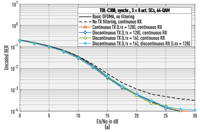
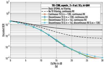
Figure 14: Performance simulation results with TDL-C $300\text{\,}\mathrm{n}\mathrm{s}$ channel and 64-QAM modulation. (a) Quasi-synchronous cases and (b) asynchronous cases (quarter-symbol timing offset). Single PRB allocated for each subband (12 SCSs, 8 active SCs, and 4 SCs for guardband).

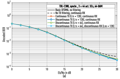
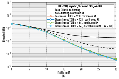
Figure 15: Performance simulation results with TDL-C $300\text{\,}\mathrm{n}\mathrm{s}$ channel and 64-QAM modulation. (a) Quasi-synchronous cases and (b) asynchronous cases (quarter-symbol timing offset). Four PRBs allocated for each subband (48 SCs, 44 active SCs, and 4 SCs for guardband).

Fig. 13(a) shows the BER simulation results for AWGN channel in synchronous scenario with single PRB per subband. In this case, the performance of the TX filtered continuous and discontinuous approaches and the RX-filtering-only scheme are practically the same. When compared with the basic synchronous OFDM, the filtered schemes have a minor performance loss. In asynchronous scenario, as depicted in Fig. 13(b), the performance of TX filtered schemes remains close to theoretical one whereas the BER floor for RX-filtering-only and basic OFDM schemes is about $0.5\text{\,}\%$ and $3\text{\,}\%$, respectively. Fig. 14(a) shows the BER simulation results for TDL-C $300\text{\,}\mathrm{n}\mathrm{s}$ channel in synchronous scenario with single PRB per subband. In this case, the channel maximum delay spread (about $2.6\text{\,}\mathrm{\SIUnitSymbolMicro s}$) is well below the CP length (about $4.7\text{\,}\mathrm{\SIUnitSymbolMicro s}$). When comparing with basic synchronous OFDM, we can see minor performance degradation of the schemes with filtering at both ends, while the degradation of the RX-filtering-only scheme is more visible. In the asynchronous case, the benefits of subband-filtered OFDM are clearly visible as illustrated in Fig. 14(b).

Fig. 15(a) compares the performance for TDL-C $300\text{\,}\mathrm{n}\mathrm{s}$ channel in synchronous scenario with four PRBs per subband. Now the performance difference between the schemes has been decreased due to the fact that, on the average, the wider subband suffer less from the interference between the subbands. The same trend can also be seen from simulation results of asynchronous scenario as shown in Fig. 15(b) where the performance degradation of RX-filtering-only and basic OFDM schemes is less obvious.

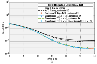
Figure 16: Performance simulation results with TDL-C $1000\text{\,}\mathrm{n}\mathrm{s}$ channel and 64-QAM modulation. (a) Quasi-synchronous cases and (b) asynchronous cases (quarter-symbol timing offset). Single PRB allocated for each subband (12 SCs, 8 active SCs, and 4 SCs guardband)

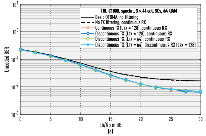
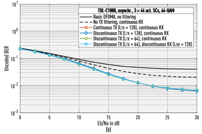
Figure 17: Performance simulation results with TDL-C $1000\text{\,}\mathrm{n}\mathrm{s}$ channel and 64-QAM modulation. (a) Quasi-synchronous cases and (b) asynchronous cases (quarter-symbol timing offset). Single PRB allocated for each subband (48 SCs, 44 active SCs, and 4 SCs for guardband)

Fig. 16(a) shows the BER simulation results for TDL-C $1000\text{\,}\mathrm{n}\mathrm{s}$ channel with single PRB per subband. In this case the channel maximum delay spread (about $8.7\text{\,}\mathrm{\SIUnitSymbolMicro s}$) exceeds the CP duration (about $4.7\text{\,}\mathrm{\SIUnitSymbolMicro s}$), resulting in higher error floor in all configurations. The same conclusions can be made as above, except that the TX filtered schemes have now better performance than the basic OFDM. The performance degradation of basic OFDM scheme is due to the inter-carrier interference (ICI) induced by the increased frequency dispersion of the channel whereas, for TX filtered OFDM, the better spectral containment provides also better protection against the ICI [25, 26]. For asynchronous scenario, as illustrated in Fig. 16(b), the performance of TX filtered schemes are approximately the same as in synchronous scenario whereas the basic OFDM and RX-filtering-only schemes have considerably higher error floors than the synchronous cases.

The BER simulation results for TDL-C $1000\text{\,}\mathrm{n}\mathrm{s}$ channel with four PRBs per subband are shown in Figs. 17(a) and (b) for synchronous and asynchronous scenarios, respectively. As seen for these figures, the performance improvement of the FC filtered waveforms remain consistent with other results.

TABLE II: Wide-band transmission scenarios and filtering configurations

Channel models	AWGN and TDL-C with $1000\text{\,}\mathrm{n}\mathrm{s}$ RMS channel delay spread
Synchronicity	Quasi-synchronous: No timing offset and no frequency offset between different uplink signals
Allocated subband width	$52\text{\,}\mathrm{\text{PRBs}}$, 624 active SCs and 8-SC guardband around the active subband
Filtering configuration	1) Continuous filtering on TX and RX sides 2) Continuous TX and discontinuous RX filtering 3) Discontinuous TX and continuous RX filtering 4) Discontinuous filtering on TX and RX sides

VI-B Bit-Error Rate Performance in Wide-band Allocations

Fig. 18 and 19 compare the simulated uncoded BER performance of continuous and discontinuous subband filtering in $10\text{\,}\mathrm{M}\mathrm{H}\mathrm{z}$ 5G-NR uplink scenario, with high-rate IFFT size of $N=1024$ and SCS of $15\text{\,}\mathrm{k}\mathrm{H}\mathrm{z}$. Single subband configuration is considered with 52 active PRBs of 12 subcarriers. In this case, eight non-active subcarriers are used as for transition bands. Table II shows details of the considered scenarios and filtering configurations. The used channel models are AWGN and TDL-C. Again two different values of the RMS channel delay spread, $300\text{\,}\mathrm{n}\mathrm{s}$ and $1000\text{\,}\mathrm{n}\mathrm{s}$, are used for TDL-C channel.

Fig. 18(a) shows the uncoded BER for QPSK, $16$-QAM, and $64$-QAM modulations. As seen from this figure, both the continuous and discontinuous processing reach the theoretical BER performance in AWGN channel. The power spectral density (PSD), as illustrated in Fig. 18(b), is about $5\text{\,}\mathrm{d}\mathrm{B}$ lower at the out-of-band region for the continuous processing when compared with discontinuous processing. The average passband EVM for continuous and discontinuous processing are $63.8\text{\,}\mathrm{d}\mathrm{B}$ and $63.4\text{\,}\mathrm{d}\mathrm{B}$, respectively.

The uncoded BER performance in TDL-C $300\text{\,}\mathrm{n}\mathrm{s}$ and $1000\text{\,}\mathrm{n}\mathrm{s}$ channels is shown in Figs. 19(a) and 19(b), respectively. As seen from Fig. 19(a), the performance of all the unfiltered and filtered schemes are approximately the same in TDL-C channel with $300\text{\,}\mathrm{n}\mathrm{s}$ delay spread. However, for channel model with maximum delay spread exceeding the CP duration as illustrated in Fig. 19(b), the pulse shaping provided by the filtering gives slightly improved performance over the plain CP-OFDM waveform.

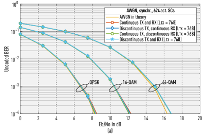
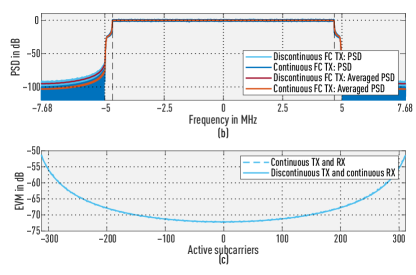
Figure 18: (a) Performance simulation results with AWGN channel and QPSK, $16$-QAM, and $64$-QAM modulations. The number of PRBs allocated for single subband is $52$ (624 active SCs and 8 SCs for guardband). In-band region (active subcarriers) is denoted by the vertical dashed lines. (b) Power spectral densities for continuous and discontinuous processing. (c) Error-vector magnitude on active subcarriers with 64-QAM modulation.

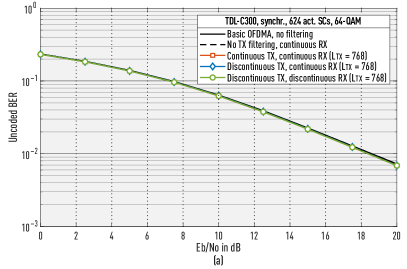
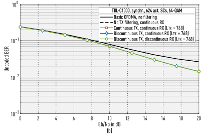
Figure 19: Performance simulation results with TDL-C $300\text{\,}\mathrm{n}\mathrm{s}$ and $1000\text{\,}\mathrm{n}\mathrm{s}$ channels and 64-QAM modulation. (a) TDL-C $300\text{\,}\mathrm{n}\mathrm{s}$ and (b) $1000\text{\,}\mathrm{n}\mathrm{s}$. The number of PRBs allocated for single subband is $52$ (624 active SCs and 8 SCs for guardband).

VI-C Implementation Complexity

Figs. 20 and 21 compare the computational complexity of different FC-based filtered OFDM schemes for different subband configurations, again in the $10\text{\,}\mathrm{M}\mathrm{H}\mathrm{z}$ 5G-NR or LTE case. The overlap factors of $\lambda=0.25$ and $\lambda=0.5$ are used for continuous processing, and $\lambda=0.5$ for discontinuous processing. The complexity is plotted as a function of the slot (TX burst) length, in the range from 1 to 14 OFDM symbols, using the number of real multiplications per transmitted QAM symbol as the complexity metric.

The short FC-transform length $L_{m}$ is equal to the IFFT length in OFDM generation and it is selected as the smallest feasible power-of-two value. Notably, the smallest value of $L_{m}$ in continuous processing is $128$, while in discontinuous processing we can use $L_{m}=16$ for single PRB ($L_{\text{act},m}=12$ subcarriers) allocation and $L_{m}=64$ for four-PRB ($L_{\text{act},m}=48$ subcarriers) allocation. In addition to the 1-PRB and 4-PRB subband cases, also the fullband allocation with 52 PRBs and $L_{\text{act},0}=624$ active subcarriers is included in the comparison.

From Figs. 20 and 21, we can observe the following:

1. Discontinuous processing for all parameterizations and slot lengths provides lower complexity than continuous processing with $50\text{\,}\%$ overlap. Discontinuous processing also provides constant complexity over different slot lengths. With short slot lengths, the complexity of discontinuous schemes is significantly lower than that of continuous transmission with $50\text{\,}\%$ overlap.

2. With multiple relatively narrow subbands, this benefit is pronounced and significant also for higher slot lengths. In these cases, the complexity of discontinuous processing is lower or similar to that of the continuous processing with $25\text{\,}\%$ overlap.

3. We remind that with $50\text{\,}\%$ overlap, the imperfections of FC processing can be ignored, while the use of $25\text{\,}\%$ overlap degrades the performance with high modulation and coding schemes.

4. The use of non-power-of-two short transform length ($L$) in building the CP-OFDM symbols and FC processing blocks may give significant complexity reduction in both continuous and discontinuous FC processing, especially in the channel filter use case. This is shown for the full-band transmission case with $L=768$ instead of $L=1024$ (channel filtering example). This transform length can be efficiently implemented by three FFTs of length $256$ and some additional twiddle factors.

5. Discontinuous processing allows to generate a single- subband signal (e.g. for NB IoT) by using the FFT size of 16 for the OFDM symbol generation and FC processing at the sampling rate of $240\text{\,}\mathrm{k}\mathrm{H}\mathrm{z}$, while prior art implementation require sampling rate of $1.92\text{\,}\mathrm{M}\mathrm{H}\mathrm{z}$ with the FFT size of 128.

The complexity evaluations for time-domain filtered OFDM and windowed overlap-and-add (WOLA) schemes and their relative complexity with respect to continuous FC processing are given in [18, 20].

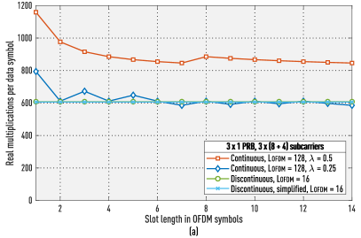
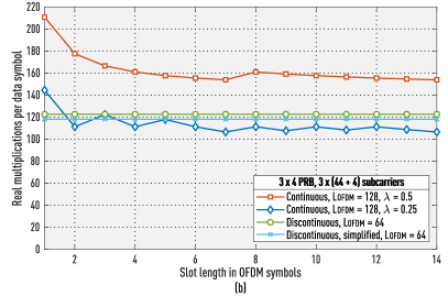
Figure 20: Computational complexity of continuous FC-F-OFDM RX processing with $25\text{\,}\%$ and $50\text{\,}\%$ overlaps and discontinuous FC-F-OFDM RX processing with $50\text{\,}\%$ overlap. (a) Three 1-PRB wide subbands. (b) Three 4-PRB wide subband.

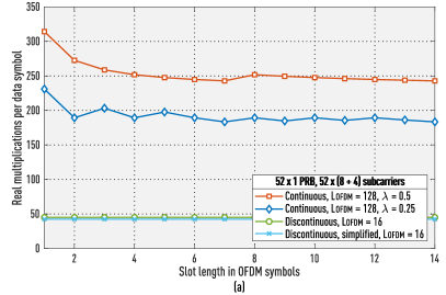
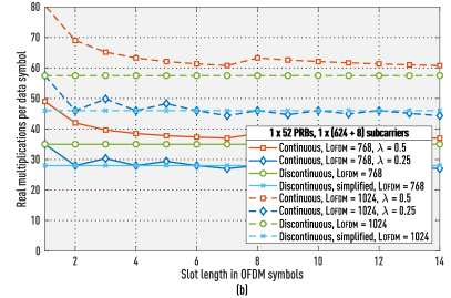
Figure 21: Computational complexity of continuous FC-F-OFDM RX processing with $25\text{\,}\%$ and $50\text{\,}\%$ overlaps and discontinuous FC-F-OFDM RX processing with $50\text{\,}\%$ overlap. (a) 52 1-PRB wide subbands. (b) Single 52-PRB wide subband.

VII Conclusions

In this article, discontinuous symbol-synchronized fast-convolution (FC) processing technique was proposed, with particular emphasis on the physical layer processing in 5G-NR and beyond mobile radio networks. The proposed processing approach was shown to offer various benefits over the basic continuous FC scheme, specifically in terms of reduced complexity and latency as well as increased parametrization flexibility. The additional inband distortion effects, stemming from the proposed scheme, were found to have only a very minor impact on the link-level performance. The benefits are particularly important in specific application scenarios, like transmission of single or multiple narrow subbands, or in mini-slot type transmission, which is a core element in the ultra-reliable low-latency transmission service of fifth-generation new radio (5G-NR).

Generally, discontinuous FC processing can be regarded as an additional useful element in the toolbox for frequency-domain waveform processing algorithms, and it can be useful for various other signal processing applications as well.

3GPP

third generation partnership project

4G

fourth generation

5G-NR

fifth-generation new radio

5G

fifth-generation

F-OFDM

subband filtered CP-OFDM

ACLR

adjacent channel leakage ratio

ADSL

asymmetric digital subscriber line

AFB

analysis filter bank

AF

amplify-and-forward

AM/AM

amplitude modulation/amplitude modulation [NL PA models]

AM/PM

amplitude modulation/phase modulation [NL PA models]

AMR

adaptive multi-rate

APP

a posteriori probability

AP

access point

AWGN

additive white Gaussian noise

B-PMR

broadband PMR

BCJR

Bahl-Cocke-Jelinek-Raviv algorithm

BER

bit error rate

BICM

bit-interleaved coded modulation

BLAST

Bell Labs layered space time [code]

BLER

block error rate

BPSK

binary phase-shift keying

BR

bin resolution

BS

bin spacing

CAZAC

constant amplitude zero auto-correlation

CB-FMT

cyclic block-filtered multitone

CCC

common control channel

CCDF

complementary cumulative distribution function

CDF

cumulative distribution function

CDMA

code-division multiple access

CFO

carrier frequency offset

CFR

channel frequency response

CH

cluster head

CIR

channel impulse response

CMA

constant modulus algorithm

CNA

constant norm algorithm

CP-OFDM

cyclic prefix orthogonal frequency-division multiplexing

CPU

central processing unit

CP

cyclic prefix

CQI

channel quality indicator

CRLB

Cramér-Rao lower bound

CRN

cognitive radio network

CRS

cell-specific reference signal

CR

cognitive radio

CSIR

channel state information at the receiver

CSIT

channel state information at the transmitter

CSI

channel state information

D2D

device-to-device

DC

direct current

DFE

decision feedback equalizer

DFT-s-OFDM

DFT-spread-OFDM

DFT

discrete Fourier transform

DF

decode-and-forward

DL

downlink

DMO

direct mode operation

DMRS

demodulation reference signals

DSA

dynamic spectrum access

DZT

discrete Zak transform

E-UTRA

evolved UMTS terrestrial radio access

ED

energy detector

EGF

extended Gaussian function

eMBB

enhanced mobile broadband

EMSE

excess mean square error

EM

expectation maximization

EPA

extended pedestrian-A [channel model]

ETSI

European Telecommunications Standards Institute

EVA

extended vehicular-A [channel model]

EVM

error vector magnitude

f-OFDM

filtered OFDM

FB-SC

filterbank single-carrier

FBMC-COQAM

filterbank multicarrier with circular offset-QAM

FBMC/OQAM

filter bank multicarrier with offset-QAM subcarrier modulation

FBMC

filter bank multicarrier

FB

filter bank

FC-F-OFDM

FC-based F-OFDM

FC-FB

fast-convolution filter bank

FC

fast-convolution

FDMA

frequency-division multiple access

FD

frequency-domain

FEC

forward error correction

FFT

fast Fourier transform

FIR

finite impulse response

FLO

frequency-limited orthogonal

FMT

filtered multitone

FPGA

field programmable gate array

FS-FBMC

frequency sampled FBMC-OQAM

FT

Fourier transform

GB

guard band

GFDM

generalized frequency-division multiplexing

GLRT

generalized likelihood ratio test

GMSK

Gaussian minimum-shift keying

HPA

high power amplifier

I/Q

in-phase/quadrature [complex data signal components]

IAM

interference approximation method

IBE

in-band emission

IBI

in-band interference

IBO

input back-off

ICI

inter-carrier interference

IDFT

inverse discrete Fourier transform

IFFT

inverse fast Fourier transform

i.i.d.

independent and identically distributed

IOTA

isotropic orthogonal transform algorithm

IoT

internet-of-things

ISI

inter-symbol interference

ITU-R

International Telecommunication Union Radiocommunication sector

ITU

International Telecommunication Union

KKT

Karush-Kühn-Tucker

KPI

key performance indicator

LE

linear equalizer

LLR

log-likelihood ratio

LMMSE

linear minimum mean squared error

LMS

least mean squares

LPSV

linear periodically shift variant

LPTV

linear periodically time-varying

LS

least squares

LTE-A

long-term evolution-advanced

LTE

long-term evolution

LUT

look-up table

MAC

medium access control

MAI

multiple access interference

MAP

maximum a posteriori

MA

multiple access relay channel

MCM

multicarrier modulation

MCS

modulation and coding scheme

MC

multicarrier

MER

message error rate

MF

matched filter

MGF

moment generating function

MIMO

multiple-input multiple-output

MISO

multiple-input single-output

MLSE

maximum likelihood sequence estimation

ML

maximum likelihood

MMA

multi-modulus algorithm

MMSE

minimum mean-squared error

MTC

massive machine-type communications

MOS

mean opinion score

MRC

maximum ratio combining

MSE

mean-squared error

MSK

minimum-shift keying

MS

mobile station

MTC

machine-type communications

MUD

multiuser detection

MUI

multiuser interference

MUSIC

multiple signal classification

MU

multi-user

NB IoT

narrow-band internet-of-things

NBI

narrowband interference

NB

narrow-band

NC-OFDM

non-contiguous OFDM

NC

non-contiguous

NL

non-linear

NMSE

normalized mean-squared error

NPR

near perfect reconstruction

NR

new radio

OBO

output back-off

OFDM

orthogonal frequency-division multiplexing

OFDMA

orthogonal frequency-division multiple access

OFDP

orthogonal finite duration pulse

OLA

overlap-and-add

OLS

overlap-and-save

OMP

orthogonal matching pursuit

OOBEM

out-of-band emission mask

OOB

out-of-band

OQAM

offset quadrature amplitude modulation

OQPSK

offset quadrature phase-shift keying

OSA

opportunistic spectrum access

PAM

pulse amplitude modulation

PAPR

peak-to-average power ratio

PA

power amplifier

PCI

perfect channel information

PER

packet error rate

PF

proportional fair

PHY

physical layer

PLC

power line communications

PMR

professional (or private) mobile radio

PPDR

public protection and disaster relief

PRB

physical resource block

ProSe

proximity services

PR

perfect reconstruction

PSD

power spectral density

PSK

phase-shift keying

PSWF

prolate spheroidal wave function

PTS

partial transmit sequence

PTT

push-to-talk

PUCCH

physical uplink control channel

PUSCH

physical uplink shared channel

PU

primary user

QAM

quadrature amplitude modulation

QoE

quality of experience

QoS

quality of service

QPSK

quadrature phase-shift keying

RAM

random access memory

RAN

radio access network

RAT

radio access technology

RBG

resource block group

RB

resource block

RC

raised cosine

RF

radio frequency

RLS

recursive least squares

RMS

root-mean-squared [error]

ROC

receiver operating characteristics

RRC

square root raised cosine

RRM

radio resource management

RSSI

received signal strength indicator

RX

receiver

SBLR

subband leakage ratio

SC-FDE

single-carrier frequency-domain equalization

SC-FDMA

single-carrier frequency-division multiple access

SCS

subcarrier spacing

SC

subcarrier

SC

single-carrier

SDMA

space-division multiple access

SDM

space-division multiplexing

SDR

software defined radio

SEL

soft envelope limiter

SER

symbol error rate

SFBC

space frequency block code

SFB

synthesis filter bank

SIC

successive interference cancellation

SIMO

single-input multiple-output

SINR

signal-to-interference-plus-noise ratio

SIR

signal-to-interference ratio

SISO

single-input single-output

SLM

selected mapping

SLNR

signal-to-leakage-plus-noise ratio

SM

spatial multiplexing

SNDR

signal-to-noise-plus-distortion ratio

SNR

signal-to-noise ratio

SI-SO

soft-input soft-output

SQP

sequential quadratic programming

SSPA

solid-state power amplifiers

SS

spectrum sensing

STBC

space time block code

STBICM

space-time bit-interleaved coded modulation

STC

space-time coding

STHP

spatial Tomlinson-Harashima precoder

SU

secondary users

SVD

singular value decomposition

TBW

transition-band width

TDD

time-division duplex

TDL

tapped-delay line

TDMA

time-division multiple access

TD

time-domain

TEDS

TETRA enhanced data service

TETRA

terrestrial trunked radio

TFL

time-frequency localization

TGF

tight Gabor frame

TLO

time-limited orthogonal

TMO

trunked mode operation

TMUX

transmultiplexer

TO

tone offset

TR

tone reservation

TSG

technical specification group

TX

transmitter

UE

user equipment

UF-OFDM

universal filtered OFDM

ULA

uniform linear array

UL

uplink

URLLC

ultra-reliable low-latency communications

V-BLAST

vertical Bell Laboratories layered space-time [code]

Veh-A

vehicular-A [channel model]

Veh-B

vehicular-B [channel model]

WiMAX

worldwide interoperability for microwave access

WLAN

wireless local area network

WLF

widely linear filter

WOLA

weighted overlap-add

WOLA

windowed overlap-and-add

ZF

zero-forcing

ZP

zero prefix

ZT

Zak transform

Juha Yli-Kaakinen received the degree of Diploma Engineer in electrical engineering and the Doctor of Technology (Hons.) degree from the Tampere University of Technology (TUT), Tampere, Finland, in 1998 and 2002, respectively. Since 1995, he has held various research positions with TUT. His research interests are in digital signal processing, especially in digital filter and filter-bank optimization for communication systems and very large scale integration implementations.

AlaaEddin Loulou received the bachelor’s degree in electrical engineering from the Islamic University of Gaza, Gaza City, Palestine, in 2006, and the M.Sc. and D.Sc. degrees in communication engineering from the Tampere University, Finland, in 2013 and 2019. He has held various research positions with Tampere University. Currently, he is working with Nokia Mobile Networks, Finland, as system on chip engineer. His current research interests include enhanced orthogonal frequency-division multiplexing waveforms and advanced multicarrier schemes.

Toni Levanen received the M.Sc. and D.Sc. degrees from Tampere University of Technology (TUT), Finland, in 2007 and 2014, respectively. He is currently with the Department of Electrical Engineering, Tampere University. In addition to his contributions in academic research, he has worked in industry on wide variety of development and research projects. His current research interests include physical layer design for 5G NR and beyond.”

Kari Pajukoski received his B.S.E.E. degree from the Oulu University of Applied Sciences in 1992. He is a Fellow with the Nokia Bell Labs. He has a broad experience from cellular standardization, link and system simulation, and algorithm development for products. He has more than 100 issued US patents, from which more than 50 have been declared “standards essential patents”. He is author or co-author of more than 300 standards contributions and 30 publications, including conference proceedings, journal contributions, and book chapters.

Arto Palin has long industrial experience in wireless technologies, covering cellular networks, broadcast systems and local area communications. He holds an MSc. (Tech.) degree from earlier Tampere University of Technology, and is currently working as Technical Leader at Nokia Mobile Networks, Finland, in the area of 5G SoC architectures.

Markku Renfors (Life Fellow, IEEE) received the D.Tech. degree from the Tampere University of Technology (TUT), Tampere, Finland, in 1982. Since 1992, he has been a Professor with the Department of Electronics and Communications Engineering, TUT, where he was the Head from 1992 to 2010. His research interests include filter-bank-based multicarrier systems and signal processing algorithms for flexible communications receivers and transmitters. Dr. Renfors was a corecipient of the Guillemin Cauer Award (together with T. Saramäki) from the IEEE Circuits and Systems Society in 1987.

Mikko Valkama (Senior member, IEEE) received the D.Sc. (Tech.) degree (with honors) from Tampere University of Technology, Finland, in 2001. In 2003, he was with the Communications Systems and Signal Processing Institute at SDSU, San Diego, CA, as a visiting research fellow. Currently, he is a Full Professor and Department Head of Electrical Engineering at newly formed Tampere University (TAU), Finland. His general research interests include radio communications, radio localization, and radio-based sensing, with particular emphasis on 5G and beyond mobile radio networks.

References

- [1] J. Yli-Kaakinen, T. Levanen, M. Renfors, M. Valkama, and K. Pajukoski, “FFT-domain signal processing for spectrally-enhanced CP-OFDM waveforms in 5G new radio,” in Proc. Asilomar Conf. Signals, Syst., Comput. (ACSSC), 2018, pp. 1049–1056.
- [2] E. Dahlman, S. Parkvall, and J. Sköld, 5G NR: The Next Generation Wireless Access Technology. Academic Press, 2018.
- [3] G. Wunder, P. Jung, M. Kasparick, T. Wild, F. Schaich, Y. Chen, S. Brink, I. Gaspar, N. Michailow, A. Festag, L. Mendes, N. Cassiau, D. Ktenas, M. Dryjanski, S. Pietrzyk, B. Eged, P. Vago, and F. Wiedmann, “5GNOW: Non-orthogonal, asynchronous waveforms for future mobile applications,” IEEE Commun. Mag., vol. 52, no. 2, pp. 97–105, Feb. 2014.
- [4] P. Banelli, S. Buzzi, G. Colavolpe, A. Modenini, F. Rusek, and A. Ugolini, “Modulation formats and waveforms for 5G networks: Who Will Be the Heir of OFDM?: An overview of alternative modulation schemes for improved spectral efficiency,” IEEE Signal Processing Mag., vol. 31, no. 6, pp. 80–93, Nov. 2014.
- [5] E. Memisoglu, A. B. Kihero, E. Basar, and H. Arslan, “Guard band reduction for 5G and beyond multiple numerologies,” IEEE Commun. Lett., vol. 24, no. 3, pp. 644–647, 2020.
- [6] H. Chen, J. Hua, F. Li, F. Chen, and D. Wang, “Interference analysis in the asynchronous f-OFDM systems,” IEEE Trans. Commun., vol. 67, no. 5, pp. 3580–3596, 2019.
- [7] J. Mao, L. Zhang, P. Xiao, and K. Nikitopoulos, “Interference analysis and power allocation in the presence of mixed numerologies,” IEEE Trans. Wireless Commun., pp. 1–1, 2020.
- [8] R. Ahmed, T. Wild, and F. Schaich, “Coexistence of UF-OFDM and CP-OFDM,” in Proc. IEEE Veh. Technol. Conf. (VTC Spring), May 2016, pp. 1–5.
- [9] X. Zhang, M. Jia, L. Chen, J. Ma, and J. Qiu, “Filtered-OFDM – Enabler for flexible waveform in the 5th generation cellular networks,” in Proc. IEEE Global Commun. Conf. (GLOBECOM), Dec. 2015, pp. 1–6.
- [10] R. Ahmed, F. Schaich, and T. Wild, “OFDM enhancements for 5G based on filtering and windowing,” in Multiple Access Techniques for 5G Wireless Networks and Beyond. Springer, Jan. 2019.
- [11] J. Li, E. Bala, and R. Yang, “Resource block filtered-OFDM for future spectrally agile and power efficient systems,” Physical Communication, vol. 14, pp. 36–55, June 2014.
- [12] R. Zakaria and D. L. Ruyet, “A novel filter-bank multicarrier scheme to mitigate the intrinsic interference: Application to MIMO systems,” IEEE Trans. Wireless Commun., vol. 11, no. 3, pp. 1112–1123, Mar. 2012.
- [13] R. Gerzaguet, D. Demmer, J.-B. Dore, and D. Kténas, “Block-filtered OFDM: A new promising waveform for multi-service scenarios,” in Proc. IEEE Int. Conf. Commun. (ICC), Paris, France, May 2017.
- [14] R. Zayani, H. Shaiek, X. Cheng, X. Fu, C. Alexandre, and D. Roviras, “Experimental testbed of post-OFDM waveforms toward future wireless networks,” IEEE Access, vol. 6, pp. 67 665–67 680, 2018.
- [15] M. Renfors, J. Yli-Kaakinen, T. Levanen, M. Valkama, T. Ihalainen, and J. Vihriälä, “Efficient fast-convolution implementation of filtered CP-OFDM waveform processing for 5G,” in Proc. IEEE Globecom Workshops, San Diego, CA, USA, Dec. 2015.
- [16] M. Renfors, J. Yli-Kaakinen, T. Levanen, and M. Valkama, “Fast-convolution filtered OFDM waveforms with adjustable CP length,” in Proc. Global Conf. Signal and Inform. Process. (GlobalSIP), Greater Washington, D.C., USA, Dec. 7–9 2016, pp. 635–639.
- [17] J. Yli-Kaakinen, T. Levanen, M. Renfors, and M. Valkama, “Optimized fast convolution based filtered-OFDM processing,” in Proc. European Conf. Networks and Commun. (EUCNC), Oulu, Finland, June 12–14 2017.
- [18] J. Yli-Kaakinen, T. Levanen, S. Valkonen, K. Pajukoski, J. Pirskanen, M. Renfors, and M. Valkama, “Efficient fast-convolution-based waveform processing for 5G physical layer,” IEEE J. Select. Areas Commun., vol. 35, no. 6, pp. 1309–1326, June 2017.
- [19] J. Yli-Kaakinen, M. Renfors, and E. Kofidis, “Filtered multicarrier transmission,” in Wiley 5G Ref: The Essential 5G reference Online, R. Tafazolli, C.-L. Wang, and P. Chatzimisios, Eds. John Wiley & Sons, Ltd., 2020, ch. 2.
- [20] J. Yli-Kaakinen, T. Levanen, A. Palin, M. Renfors, and M. Valkama, “Generalized fast-convolution-based filtered-OFDM: Techniques and application to 5G New Radio,” IEEE Trans. Signal Processing, vol. 68, pp. 1309–1326, 2020.
- [21] Technical Specification Group Radio Access Network; Evolved Universal Terrestrial Radio Access (E-UTRA); Base Station (BS) Radio Transmission and Reception (Release 16), document TS 36.104 V16.2.0, 3GPP, June 2019.
- [22] Technical Specification Group Radio Access Network; NR; Base Station (BS) Radio Transmission and Reception (Release 16), document TS 38.104 V16.0.0, 3GPP, June 2019.
- [23] H. Sorensen, M. Heideman, and C. Burrus, “On computing the split-radix FFT,” IEEE Trans. Acoust., Speech, Signal Processing, vol. 34, no. 1, pp. 152–156, Feb. 1986.
- [24] Technical Specification Group Radio Access Network; Study on channel model for frequency spectrum above 6 GHz (Release 15), document TR 38.900 V15.0.0, 3GPP, June 2018.
- [25] T. Strohmer and S. Beaver, “Optimal OFDM design for time-frequency dispersive channels,” IEEE Trans. Commun., vol. 51, no. 7, pp. 1111–1122, July 2003.
- [26] Z. Zhao, M. Schellmann, X. Gong, Q. Wang, R. Böhnke, and Y. Guo, “Pulse shaping design for OFDM systems,” EURASIP J. Wirel. Comm., vol. 2017, no. 2017:74, pp. 1–25, 2017.