Test of analyticity and unitarity for the pion form-factor data around the $\rho$ resonance

Abstract

High-statistics data on the $e^{+}e^{-}\to\pi^{+}\pi^{-}$ cross section and the pion vector form factor have been obtained recently by several collaborations. Unfortunately, there are some tensions between different datasets, especially the most precise ones, which have not been resolved so far. Additional independent constraints on the data are therefore of interest. We consider a parametrization-free method of analytic extrapolation proposed recently, which is based on a mixed phase and modulus extremal problem and combines rigorous upper and lower bounds with numerical simulations to account for the statistical distributions of the input and output values. Spacelike data on the form factor and measurements of the modulus in the region $(0.65-0.71)\,\text{GeV}$ are used as input. In previous works, the formalism was applied for extrapolating the form factor to low energies. In the present work, we use it as a stringent and model-independent test of consistency with analyticity and unitarity for the high-statistics data around the $\rho$ resonance. The study reveals some inconsistencies, in particular below the $\rho$ peak the BABAR data are slightly higher than the band of extrapolated values, while above the $\rho$ peak all the data are situated at the lower edge of the band. The implications of the results on the two-pion vacuuum polarization contribution to the anomalous magnetic moment of the muon are briefly discussed.

I Introduction

The electromagnetic form factor $F_{\pi}^{V}(t)$ of the pion is a fundamental quantity for strong-interaction physics, intensively studied theoretically and experimentally for more than sixty years. The recent interest in its precise determination is mostly driven by the anomalous magnetic moment of the muon, $a_{\mu}=(g-2)_{\mu}/2$. There is at present a disagreement between the experimental value of the muon anomaly measured at BNL Bennett:2006fi and its evaluation in the Standard Model (SM). Two new experiments aim at reducing the experimental uncertainty by a factor of four: the E989 experiment at Fermilab Grange:2015fou , which started running in 2018, and the E34 experiment at J-PARC, which plans to start its first run in 2024 Abe:2019thb . In parallel, there is a continuous effort for improving the accuracy of the theoretical calculation of $a_{\mu}$ in the SM (for a recent review and earlier references see Aoyama:2020ynm ).

The hadronic vacuum polarization (HVP) contribution to the muon $g-2$ is the leading hadronic contribution, which cannot be calculated using perturbative QCD and dominates the theoretical uncertainty. By analyticity and unitarity, the hadronic loops contribute to leading order (LO) as a dispersion integral over the cross section of the $e^{+}e^{-}$ annihilation into hadrons. This allows a data-driven evaluation of HVP using experimental data (the most recent determinations are reported in Davier:2019can ; Keshavarzi:2019abf ; Aoyama:2020ynm ). At low energies, below $\sqrt{s}=1\,\text{GeV}$, the dispersive integral is dominated by the cross section of the $e^{+}e^{-}$ annihilation into two pions. Several high-statistics $e^{+}e^{-}$ experiments Akhmetshin:2003zn -Ablikim:2015orh have been designed and operated recently in order to measure this quantity with increased precision. However, as noted in Davier:2019can ; Keshavarzi:2019abf ; Aoyama:2020ynm , there are some tensions between the data of different experiments, particularly the most precise ones, BABAR Aubert:2009ad ; Lees:2012cj and KLOE Ambrosino:2008aa ; Ambrosino:2010bv ; Babusci:2012rp .

It is useful to keep in mind that to LO the cross section of the $e^{+}e^{-}\to\pi^{+}\pi^{-}$ process is expressed in terms of the modulus squared of the pion vector form factor, $F_{\pi}^{V}(t)$. This allows, in principle, to use additional theoretical and experimental information available on the form factor in order to improve the accuracy, especially in regions where the data are still poor. The most powerful approach for the study of the form factor is dispersion theory, which exploits analyticity, unitarity and crossing symmetry. The form factor has been calculated also on the lattice, but the results did not reach the same accuracy until now, and we shall not consider them.

The dispersion theory of the pion form factor traditionally exploits Fermi-Watson theorem Fermi:2008zz ; Watson:1954uc , which states that below the first inelastic threshold the phase of the form factor on the unitarity cut is equal to the $P$-wave phase shift of $\pi\pi$ elastic scattering. By the well-known Omnès representation, the form factor is reconstructed as an analytic function in the whole complex $t$-plane from its phase of the boundary. The most recent dispersive analysis Colangelo:2018mtw is based on a parametrization involving an Omnès function multiplied by factors which account for inelastic and isospin-breaking effects. The $P$-wave $\pi\pi$ phase shift used as input was obtained by solving Roy equations, which fully exploit analyticity, unitarity and crossing symmetry of pion-pion scattering amplitudes, and the free parameters of the model have been fixed by fitting data on the modulus of the form factor from $e^{+}e^{-}$ experiments.

As noted in Colangelo:2018mtw , in the combined fit of all data one can observe the well-known tension between the BABAR and KLOE data: the BABAR data lie systematically above the KLOE data. The fit follows the average of the two in accordance with their respective covariance matrices. In the Omnès representation used in Colangelo:2018mtw , an assumption about the phase in the inelastic region, where it is not known, has been adopted. Actually, the parametrization contains an additional factor, which is complex above the inelastic threshold and can modify the initial phase. However, the independence of the results on the choice of the phase in the Omnès function is not formally proved.

As remarked for the first time in Caprini:1999ws , in order to avoid assumptions on the unknown phase in the inelastic region, one can use instead the phase some information available in this region on the modulus. This leads to a mixed phase and modulus representation, which can be generalized by including also an arbitrary number of values of the form factor at points inside the analyticity domain. The price to be paid for the independence on the unknown phase above the inelastic threshold is that the formalism cannot predict definite values, but only upper and lower bounds on the form factor. The bounds can be calculated exactly with techniques of functional analysis in terms of the information used as input (for technical detail see Abbas:2010jc ; Caprini:2019osi ).

An important step forward was achieved in Refs. Ananthanarayan:2016mns ; Ananthanarayan:2017efc ; Ananthanarayan:2018nyx ; Ananthanarayan:2019zic , where the rigorous bounds derived from analyticity have been merged with numerical simulations which properly take into account the statistical distribution of the input and output values. This elaborate formalism has been applied for the determination of the pion charge radius Ananthanarayan:2017efc and the modulus of the form factor at low energies Ananthanarayan:2016mns ; Ananthanarayan:2018nyx ; Ananthanarayan:2019zic . In particular, a more accurate value of the HVP contribution to $a_{\mu}$ from energies below 0.63 GeV has been obtained. The input used in these works consisted from the most recent measurements of the form factor in the spacelike region and the data on the modulus measured in the range of $(0.65-0.71)\,\text{GeV}$, where the various experiments are in somewhat better mutual agreement than in other regions.

In principle, the method can be used to predict the form factor also at higher energies, above 0.71 GeV, up to the first inelastic threshold. However, as will be clear below, the analyticity bounds become gradually weaker at energies far from the input range, especially when the inelastic threshold is approached. Therefore, unlike the low-energy region where the predictions have been more precise than the experimental data, above the $\rho$-resonance region, where precise data by high statistics experiments are available, we do not expect our determinations to compete with them in precision. However, the formalism is still useful since it provides a stringent test of consistency of the form-factor data with analyticity and unitarity.

The purpose of the present work is to explore the outcome of this test for energies below and above the $\rho$ resonance. The paper is organized as follows: in the next section, we give a brief description of the formalism, expressing it as a parametrization-free test of consistency for the values of the form factor at various energies. In Sec. III we describe the theoretical and phenomenological information used as input and the methodology for extrapolating the form factor in the output region. In Sec. IV we present our results, confronting the extrapolated values with the experimental data in the region $(0.72-0.9)\,\text{GeV}$ as the modulus input are taken from the region $(0.65-0.71)\,\text{GeV}$. A discussion of the results, in particular of their implication on the HVP contribution to the muon $g-2$, is given in Sec. V. The paper has an Appendix, which contains an explicit proof of the independence of the results on the unknown phase of the form factor above the inelastic threshold.

II Parametrization-free analyticity and unitarity constraints

The pion vector form factor $F_{\pi}^{V}(t)$ is an analytic function in the complex $t$ plane cut along the real range $t\geq t_{+}$, where $t_{+}=4m_{\pi}^{2}$. It satisfies the Schwarz reflection property $F_{\pi}^{V}(t^{*})=(F_{\pi}^{V}(t))^{*}$ and the normalization $F_{\pi}^{V}(0)=1$.

Along the cut the form factor is a complex function. According to Fermi-Watson theorem Fermi:2008zz ; Watson:1954uc , below the first inelastic threshold the phase of the form factor is equal to the $P$-wave phase shift $\delta_{1}^{1}(t)$ of the $\pi\pi$ elastic scattering. Since this theorem is valid in the exact isospin limit, we must first remove the main isospin-violating effect, known to arise from $\omega-\rho$ and $\phi-\rho$ interference.

We shall follow the standard approach Leutwyler:2002hm ; Hanhart:2012wi ; Colangelo:2018mtw to do this, by defining a purely $I=1$ function $F(t)$ as

$$F(t)=F_{\pi}^{V}(t)/F_{\omega+\phi}(t),$$ (1)

where the function $F_{\omega+\phi}(t)$, specified in the next section, includes the $I=0$ contribution due to $\omega$ and $\phi$ resonances. Then Fermi-Watson theorem allows us to write

$$\arg F(t+i\epsilon)=\delta_{1}^{1}(t),\quad\quad 4m_{\pi}^{2}\leq t\leq t_{in},$$ (2)

where one can assume with a good approximation that the first inelastic threshold is set up by the $\omega\pi$-production threshold, and take $\sqrt{t_{in}}=m_{\omega}+m_{\pi}=0.917\,\text{GeV}$. In the elastic region, the phase shift $\delta_{1}^{1}(t)$ is known with high precision from dispersion theory for $\pi\pi$ scattering Ananthanarayan:2000ht ; Caprini:2011ky ; GarciaMartin:2011cn .

Above $t_{in}$, where the phase of the form factor is not known, we use the information available on the modulus from experimental measurements and perturbative QCD. Specifically, we adopt a conservative condition written as

$$\frac{1}{\pi}\int_{t_{in}}^{\infty}|F_{\pi}^{V}(t)|^{2}\frac{dt}{t}\leq I$$ (3)

where the integral converges and allows an accurate evaluation of $I$ from the available information.

From the phase and modulus conditions (2) and (3), using techniques of functional analysis and optimization theory (for a review see Caprini:2019osi ), one can derive constraints on the values of the form factor and its derivatives at points inside the analyticity domain. Omitting the proof given in Abbas:2010jc ; Caprini:2019osi (see also the Appendix of Ananthanarayan:2018nyx ), we shall write down these constraints in a compact form, by expressing the form factor in the isospin limit as

$$F(t)=\frac{{\cal{O}}(t)}{\omega(t)}\,\frac{g(\tilde{z}(t))}{w(\tilde{z}(t))},$$ (4)

where

$${\cal{O}}(t)=\exp\left(\displaystyle\frac{t}{\pi}\int^{\infty}_{t_{+}}dt^{\prime}\displaystyle\frac{\phi(t^{\prime})}{t^{\prime}(t^{\prime}-t)}\right),$$ (5)

$$\omega(t)=\exp\left(\displaystyle\frac{\sqrt{t_{in}-t}}{\pi}\int^{\infty}_{t_{in}}\displaystyle\frac{\ln|{\cal{O}}(t^{\prime})|\,{\rm d}t^{\prime}}{\sqrt{t^{\prime}-t_{in}}(t^{\prime}-t)}\right),$$ (6)

$$w(z)=\sqrt{\frac{1-z}{1+z}},$$ (7)

and the function

$$\tilde{z}(t)=\frac{\sqrt{t_{in}}-\sqrt{t_{in}-t}}{\sqrt{t_{in}}+\sqrt{t_{in}-t}}$$ (8)

conformally maps the $t$ complex plane cut for $t\geq t_{in}$ onto the unit disk $|z|<1$, such that $\tilde{z}(0)=0$ and the upper(lower) edges of the cut become the upper(lower) semicircles in the $z$ plane.

We recall that ${\cal{O}}(t)$ is an Omnès function, where $\phi(t)$ is equal to $\delta_{1}^{1}(t)$ for $t\leq t_{in}$ and is an arbitrary function above $t_{in}$. The function denoted as $\omega(t)$ is analytic in the $t$ plane cut for $t>t_{in}$ and has the modulus equal to $|{\cal{O}}(t)|$ on the cut, and $w(z)$ is an outer function (analytic and without zeros in the unit disk $|z|<1$), with modulus on the boundary $|z|=1$ of the disk related to to the weight in the integral (3).

Finally, the function $g(z)$ appearing in (4) is an analytic function in the disk $|z|<1$ and satisfies the boundary condition

$$\frac{1}{2\pi}\int^{2\pi}_{0}{\rm d}\theta|g(\zeta)|^{2}\leq I,\qquad\zeta=e^{i\theta}.$$ (9)

This condition implies rigorous correlations among the values of the function $g(z)$ and its derivatives at points inside the holomorphy domain, $|z|<1$. In particular, if $z_{n}\in(-1,1)$, $n=1,\,2,\,3$ are three arbitrary real points, the following positivity condition holds

$${\cal D}\geq 0$$ (10)

where ${\cal D}$ is the determinant defined as

$${\cal D}=\left|\begin{array}[]{c c c c c c}I-g(0)^{2}&\xi_{1}&\xi_{2}&\xi_{3}\\ \xi_{1}&\displaystyle\frac{z^{2}_{1}}{1-z^{2}_{1}}&\displaystyle\frac{z_{1}z_{2}}{1-z_{1}z_{2}}&\displaystyle\frac{z_{1}z_{3}}{1-z_{1}z_{3}}\\ \xi_{2}&\displaystyle\frac{z_{1}z_{2}}{1-z_{1}z_{2}}&\displaystyle\frac{z_{2}^{2}}{1-z_{2}^{2}}&\displaystyle\frac{z_{2}z_{3}}{1-z_{2}z_{3}}\\ \xi_{3}&\displaystyle\frac{z_{1}z_{3}}{1-z_{1}z_{3}}&\displaystyle\frac{z_{2}z_{3}}{1-z_{2}z_{3}}&\displaystyle\frac{z_{3}^{2}}{1-z_{3}^{2}}\\ \end{array}\right|,$$ (11)

where

$$g(0)=w(0)\omega(0)/{\cal{O}}(0),$$ (12)

and

$$\xi_{n}=g(z_{n})-g(0),\quad 1\leq n\leq 3.$$ (13)

Moreover, the principal minors of the determinant ${\cal D}$ must also be nonnegative. We emphasize that the normalization condition $F_{\pi}^{V}(0)=1$ is included as input and is implemented in the definition of $g(0)$ in (12).

The inequality (10) defines an allowed domain for the real values $g(z_{n})$, which can be expressed in a straightforward way in terms of the values of the form factor at the points $t_{n}=\tilde{t}(z_{n})$, where

$$\tilde{t}(z)=t_{in}\,\frac{4z}{(1+z)^{2}}$$ (14)

is the inverse of (8).

In particular, for $t_{n}<t_{+}$, when both $F(t_{n})$ and ${\cal{O}}(t_{n})$ are real, we have from (4):

$$g(z_{n})=F(t_{n})w(z_{n})\,\omega(t_{n})/{\cal{O}}(t_{n}),$$ (15)

while for $t_{+}<t_{n}<t_{in}$, when $F(t_{n})$ and ${\cal{O}}(t_{n})$ are complex and have equal phases,

$$g(z_{n})=|F(t_{n})|w(z_{n})\,\omega(t_{n})\,/|{\cal{O}}(t_{n})|,$$ (16)

where the modulus $|{\cal{O}}(t)|$ of the Omnès function is obtained from (5) by the principal value (PV) Cauchy integral

$$|{\cal{O}}(t)|=\exp\left(\frac{t}{\pi}\text{\rm PV}\int^{\infty}_{t_{+}}dt^{\prime}\displaystyle\frac{\phi(t^{\prime})}{t^{\prime}(t^{\prime}-t)}\right).$$ (17)

Using these relations, the inequality (11) can be written as an explicit consistency test imposed by anayticity on the values $F(t_{n})$ at three arbitrary points below $t_{in}$. As proved in Abbas:2010jc ; Caprini:2019osi , the constraint exploits in an optimal way the input information. Moreover, although the function ${\cal{O}}(t)$ depends on the phase $\phi(t)$ for $t>t_{in}$, the test is independent on it. For completeness, we give in the Appendix, along with the formal argument put forward in Caprini:1999ws ; Abbas:2010jc , an explicit proof of this independence, presented here for the first time.

III Determination of $|F_{\pi}^{V}|$ in the $\rho$ region

In our analysis, we have treated two of the values of $F(t)$ in (11) as input, using experimental information on the form factor (or its modulus) at two points on the spacelike and timelike axes. For each input, the inequality (10) becomes a quadratic constraint on the form factor at the third point, from which upper and lower bounds are exactly derived. The test will consist from the comparison of these bounds with the experimental data available in the third region. The regions used as input and output will be specified below.

III.1 Inputs

We have extracted the pion form factor from the cross section of the $e^{+}e^{-}\to\pi^{+}\pi^{-}$ process using standard correction factors (see for instance Appendix B of Ananthanarayan:2016mns ). We then converted the input values of $F_{\pi}^{V}(t)$ into the isospin-conserving function $F(t)$ using (1), solved the optimization problem for this function and finally re-expressed the results in terms of $|F_{\pi}^{V}(t)|$. The function $F_{\omega+\phi}(t)$, which accounts for the isospin violation due to $\omega-\rho$ and $\phi-\rho$ mixing, has been taken of the form Leutwyler:2002hm ; Hanhart:2012wi :

$$F_{\omega+\phi}(t)=1+\frac{\epsilon\,t}{t-(m_{\omega}-i\Gamma_{\omega}/2)^{2}}+\frac{\epsilon^{\prime}\,t}{t-(m_{\phi}-i\Gamma_{\phi}/2)^{2}},$$ (18)

where $\epsilon=-2\times 10^{-3}$, $\epsilon^{\prime}=5\times 10^{-3}$ and the masses and the decay widths are taken as $m_{\omega}=781.86$, $m_{\phi}=1019.46\,\text{MeV}$, $\Gamma_{\omega}=8.5\,\text{MeV}$ and $\Gamma_{\phi}=4.3\,\text{MeV}$ Tanabashi:2018oca .

We have taken the phase shift $\delta_{1}^{1}(t)$ entering the integral (5) below $t_{in}$ from Ananthanarayan:2000ht ; Caprini:2011ky (Bern phase) and GarciaMartin:2011cn (Madrid phase). They have been calculated with good precision using dispersion relations for $\pi\pi$ scattering and are mutually consistent, with slightly larger uncertainties of the Bern phase near $t_{in}$. Above $t_{in}$ we have taken for $\phi(t)$ an arbitrary expression. As we have already mentioned, the results are independent of this arbitrariness. The proof of this is provided in Appendix A.

We have calculated the integral (3) using the BABAR data Aubert:2009ad from $t_{in}$ up to $\sqrt{t}=3\,\text{GeV}$, smoothly continued with a constant value for the modulus in the range $3\,\text{GeV}\leq\sqrt{t}\leq 20\,\text{GeV}$, and a decrease $\sim 1/t$ at higher energies, as predicted by perturbative QCD Farrar:1979aw ; Lepage:1979zb . With this input we have obtained $I=0.578\pm 0.022$, where the uncertainty is due to the BABAR experimental errors. In the calculations we have used as input for $I$ the central value increased by the error, which leads to the most conservative bounds due to a monotonicity property discussed in Ananthanarayan:2016mns .

The input at interior points was taken from the most recent experimental measurements of $F_{\pi}$ Collaboration at JLab Horn:2006tm ; Huber:2008id on the spacelike axis,

$$F_{\pi}^{V}(-1.60\,\text{GeV}^{2})=0.243\pm 0.012_{-0.008}^{+0.019},$$

$$F_{\pi}^{V}(-2.45\,\text{GeV}^{2})=0.167\pm 0.010_{-0.007}^{+0.013},$$ (19)

and the modulus measured by the $e^{+}e^{-}$ experiments SND (04), CMD2 (06), BABAR (09), KLOE (11), KLOE (13) and BESIII (15) Akhmetshin:2003zn -Ablikim:2015orh in the region $(0.65-0.71)\,\text{GeV}$ on the timelike axis.

The choice of the input region $(0.65-0.71)\,\text{GeV}$ was motivated in our previous works Ananthanarayan:2016mns ; Ananthanarayan:2017efc ; Ananthanarayan:2018nyx by the fact that here the data have a better precision than at the lower energies where we extrapolated the form factor . The number of input points in this region from each experiment is given in Table 1 of Ref. Ananthanarayan:2016mns . We adopt the same input region in the present work, since the determinations of different experiments, especially the most precise ones, BABAR and KLOE, are more consistent among them in this region than at higher energies, around the $\rho$ resonance (see for instance the comparisons in Fig. 13 of Aoyama:2020ynm ).

We recall that the hadronic decays of $\tau$ leptons have been used in the past as an alternative source of data in the evaluation of the HVP contribution to $a_{\mu}$. Isospin-breaking (IB) and electromagnetic corrections must be applied in order to convert these data to the cross section of $e^{+}e^{-}$ annihilation (for a recent evaluation and earlier references see 1808470 ). However, as remarked in Aoyama:2020ynm , the present understanding of these corrections is not yet at a level allowing the use of $\tau$ data in the muon $g-2$ determinations. In view of this consensus in the community, in this work we will use only $e^{+}e^{-}$ data.

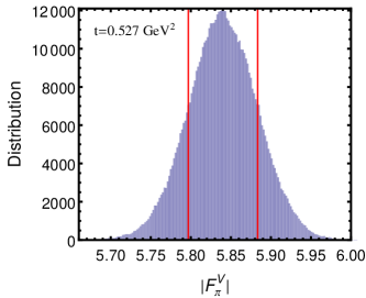
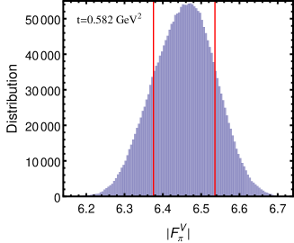
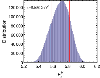
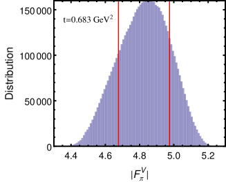
Figure 1: Statistical distribution of $|F_{\pi}^{V}(t)|$ at different energies $t$ shown in the legends. To obtain these histogram we use modulus data at $0.699\,\text{GeV}$ measured by BABAR, the spacelike point $t_{s}=-1.6\,\text{GeV}^{2}$, and Bern phase. The vertical lines (red) correspond to 68.3% CL intervals.

III.2 Methodology of $|F_{\pi}^{V}|$ determination

We have taken the range $(0.72-0.9)\,\text{GeV}$ as the output region, where we extrapolate the form factor and confront the results with the experimental data.

A nontrivial complication is the fact that the experimental values used as input are known up to statistical and systematic uncertainties. This requires to properly merge the formalism of analytic bounds with statistical simulations. The problem was solved in Refs. Ananthanarayan:2016mns ; Ananthanarayan:2017efc ; Ananthanarayan:2018nyx by generating a large sample of pseudodata, achieved by randomly sampling each of the input quantities with specific distributions based on the measured central values and the quoted errors. For each point from an input statistical sample, upper and lower bounds on $|F_{\pi}^{V}(t)|$ at points $t$ in the output region have been calculated using the formalism described in the previous section. Note that the input points had to pass a consistency condition in order to be included in the sample. Indeed, some of the minors of the determinant ${\cal D}$, mentioned below (13), involve only input quantities and, if the positivity condition is violated, the corresponding points had to be rejected. Finally, a set of allowed values in between the bounds has been uniformly generated, taking into account the fact that all the values between the extreme points are equally valid. The number of generated points was adapted to the width of the allowed range, being larger fow wider ranges.

In this way, for a specified spacelike and timelike input, we generated a large sample of output values of $|F_{\pi}^{V}(t)|$ at each point $\sqrt{t}$ in range $(0.72-0.9)\,\text{GeV}$ of interest. The output distributions turn out to be close to a Gaussian, allowing the extraction of the mean value and the standard deviation (defined as the 68.3% confidence limit interval). The values obtained with input from each experiment at different energies and of the different experiments (SND, CMD2, BABAR, KLOE11, KLOE13 and BESIII) have been then combined using an averaging prescription proposed in Schmelling:1994pz , where the correlations between different values are derived from the values themselves. The two spacelike input points have been considered separately and then we took the average of the two predictions for both the central value and the error. The same conservative procedure has been adopted for the phases: we considered the results obtained separately with the Bern and Madrid phases and also the simple average of the corresponding predictions. The comparison of these results with the experimental values serves as a test of unitarity and analyticity of the experimental determinations in the input and output regions.

IV Results

We start by illustrating the statistical distributions of the output values of $|F_{\pi}^{V}(t)|$, obtained with a specific input. In Figs. 1 we show these distributions at several values of $t$, obtained with the pseudodata sample generated with the experimental measurement at $0.699\,\text{GeV}$ by BABAR, the first spacelike input (III.1) and Bern phase. One can note the increasing number of points in the samples with increasing $t$. The explanation is that the allowed bands between the upper and lower bounds become wider at larger energies, and more intermediate points must be generated in order to obtain the correct statistical distribution. All the distributions are very close to a Gaussian, allowing the extraction of a central value and a standard deviation at 68.3% confidence level.

From these distributions, by applying the averaging procedure described in Sec. III.2, we obtained a central value and a standard deviation for the modulus for all energies in the output region $(0.72-0.9)\,\text{GeV}$. For convenience, we present the extrapolated values of $|F_{\pi}^{V}(t)|^{2}$ at 68.3% CL in this region as a band denoted as “allowed band”. This is the main prediction of our method, which we compare with the experimental values available in the same region.

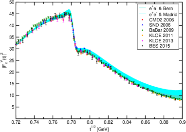
Figure 2: Allowed bands of $|F_{\pi}^{V}(t)|^{2}$ at 68.3% CL obtained with input from all $e^{+}e^{-}$ experiments. The bands obtained with the Bern and Madrid phases are shown separately.

In Fig. 2 we show the allowed bands for $|F_{\pi}^{V}(t)|^{2}$ in the range $(0.72-0.9)\,\text{GeV}$, obtained by using as input all $e^{+}e^{-}$ experiments (SND, CMD2, BABAR, KLOE 11, KLOE 13 and BESIII) in comparison with the $e^{+}e^{-}$ experimental data in the same region. The bands obtained with the Bern and Madrid phases are shown separately.

Several remarks can be made from this figure. First, below the $\rho$ peak the bands of extrapolated values are rather narrow, competing with the experimental data in this region. Only BABAR and KLOE data are more precise than the prediction. Several BABAR points lie definitely above the allowed band, while several KLOE points lie below the band. We can say that these points are in certain tension with analyticity and the data from the lower-energy region, $(0.65-0.71)\,\text{GeV}$. For the other datasets, which have larger uncertainties, no inconsistencies are seen.

Above the $\rho$ peak, the allowed bands obtained by extrapolation become gradually wider, as anticipated, and cannot compete in precision with the experimental data. However, some interesting features can be seen also in this region. All the data lie at the lower edge of the wider band obtained with the Bern phase Caprini:2011ky , and are definitely below the band obtained with the Madrid phase GarciaMartin:2011cn , which is more narrow since the quoted uncertainties are smaller. Some experimental points near 0.9 GeV are also below the average band obtained with the two phases, presented in Fig. 3.

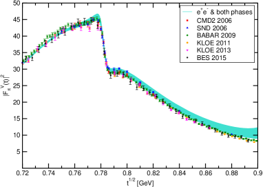
Figure 3: Allowed band obtained with input from all $e^{+}e^{-}$ experiments and Bern and Madrid phases.

The above predictions have been obtained by using as input all the data in the range $(0.65-0.71)\,\text{GeV}$. It is of interest to see what happens if we restrict the input to some datasets. In Fig. 4 we show the allowed band obtained using as input only BABAR 2009 data Aubert:2009ad and Bern phase. One can see that now the BABAR points below the $\rho$ peak are in more agreement with the allowed band, while the KLOE data lie definitely below the band and above the $\rho$ peak all the experimental data are well below the allowed band. As an opposite choice, we show in Fig. 5 the allowed band obtained using as input all the data except BABAR, with Bern phase used as before. The data are now in more agreement with the allowed band, except the BABAR data below the $\rho$ peak which are definitely higher.

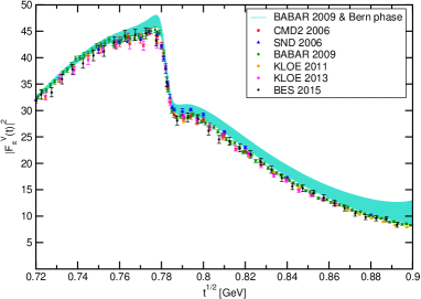
Figure 4: Allowed band using as input only BABAR data and Bern phase.

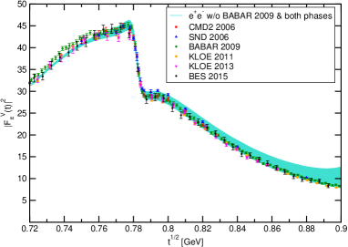
Figure 5: Allowed band using as input $e^{+}e^{-}$ data without BABAR, and Bern phase.

Finally, in Figs. 6 and 7 we present the allowed bands obtained using as input only KLOE 2011 Ambrosino:2010bv and KLOE 2013 Babusci:2012rp data, respectively, and Bern phase. Now all the experimental points, below and above the $\rho$ peak, are inside the allowed range, except the BABAR data below the $\rho$ peak, which are clearly above it. We note that the disagreement is more pronounced for the KLOE 2011 input, and slightly less stringent for the KLOE 2013 input.

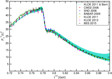
Figure 6: Allowed band using as input only KLOE11 data and Bern phase.

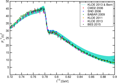
Figure 7: Allowed band using as input only KLOE13 data and Bern phase.

V Discussion and conclusions

In the present paper we have investigated the consistency of the recent high-statistics experimental data on the pion vector form factor with analyticity and unitarity. The aim was to provide additional constraints on the dispersive evaluation of the HVP contribution to the SM value of the muon $g-2$. The work was motivated also by the tensions which exist between the most precise data, BABAR and KLOE, which have not been resolved so far.

We have used a model-independent formalism, which uses Fermi-Watson theorem (2) in the elastic region and a very conservative integral condition (3) on the modulus in the inelastic region. From these boundary conditions, rigorous constraints on the values of the form factor at points inside the analyticity domain can be derived, expressed in the particular case of three points as the positivity condition (10) of the determinant (11) and of its minors.

In our analysis, we have exploited this constraint by using as input the experimental data (III.1) on the form factor on the spacelike axis and the measurements of the modulus in the region $(0.65-0.71)\,\text{GeV}$ by the SND, CMD2, BABAR, KLOE 11, KLOE 13 and BESIII experiments. The choice of this region was justified by the fact that data from various experiments are here in better mutual agreement than at higher energies. It may be noted however that this choice is an educated guess and cannot necessarily be considered very rigorous. In particular, some tensions between BABAR and KLOE data exist even in this region.

Using a specific input, we have derived upper and lower bounds on the modulus in the higher-energy region $(0.72-0.9)\,\text{GeV}$, which includes the $\rho$ peak. The bounds derived from analyticity have been converted into central values and standard deviations at 68.2% CL by using numerical simulations on pseudodata samples, and have been presented as a band of “allowed values”. The aim was to compare the bands obtained by analytic extrapolation with the experimental data available in the same region, where the tensions between BABAR and KLOE are larger.

We emphasize that in the present formalism the analytic extrapolation is performed without a specific parametrization of the form factor, like the Gounaris-Sakurai formula or the Omnès-like parametrizations used in the literature. Moreover, the results are optimal for a definite input and are rigorously independent on the unknown phase of the form factor above the inelastic threshold. For completeness, we gave in the Appendix A formal argument and a detailed proof of this property, presented here for the first time.

The results presented in Sec. IV indicate some inconsistencies between the data and the extrapolated band. The tension between BABAR and KLOE is manifest and exhibits new facets. As shown in Fig. 4, using as input only BABAR data in the region $(0.65-0.71)\,\text{GeV}$, the KLOE data below the $\rho$ peak are definitely lower than the extrapolated band. More impressively, above the $\rho$ peak all the data, including BABAR, lie below the allowed band. If, on the other hand, only KLOE data in the region $(0.65-0.71)\,\text{GeV}$ are used as input, Figs. 6 and 7 show that all the data above 0.72 GeV are consistent with the allowed band, except for BABAR data below the $\rho$ peak, which lie definitely above the band.

A somewhat surprising feature is that all the data above the $\rho$ peak appear to be situated at the lower edge of the extrapolated band. This feature is more dramatic when only BABAR data in the region $(0.65-0.71)\,\text{GeV}$ are used as input, as seen in Fig. 4, but is obtained also with input from all experiments, or from all experiments except BABAR, as seen in Figs. 3 and 5, respectively.

It is difficult at present to find a simple explanation for this result. Thus, it is unlikely that the resolution of the puzzle lies in insufficient knowledge of the phase. An important ingredient in our approach is the phase shift $\delta_{1}^{1}$, but this function is calculated with precision in $\pi\pi$ dispersion theory. Moreover, we used two phases, calculated independently in Caprini:2011ky and GarciaMartin:2011cn , and the results are consistent, with a somewhat wider bands obtained with Bern phase, which has larger uncertainties near 0.9 GeV.

A global correction factor, with large values precisely in the region of interest, might offer a possible explanation. We recall in this context the so-called $\rho-\gamma$ mixing factor, calculated in Jegerlehner:2011ti , whose effect is to slightly push upward the modulus of the form factor extracted from $e^{+}e^{-}$ data above the $\rho$ peak. However, for the moment we refrain from further speculating on possible explanations of the fact that the data from the region $(0.65-0.71)\,\text{GeV}$ seem to require higher values than the experimental measurements of the modulus above the $\rho$ peak, especially above 0.8 GeV.

Instead, we briefly comment on the implications of this result on the HVP contribution to the muon $g-2$. As it is known, the two-pion LO contribution to $a_{\mu}$, which does not contain the vacuum polarization effects but includes one-photon final-state radiation (FSR), is expressed as an integral over the modulus squared on the pion form factor (for the explicit formulae see for instance Sec. II of Ananthanarayan:2016mns ).

Using the central value and the error of the extrapolated band shown in Fig. 3, we obtained for the contribution from the region $[0.8,\,0.9]\,\text{GeV}$ the value $a_{\mu}[0.8,\,0.9]=(70\pm 4)\times 10^{-10}$. On the other hand, the values obtained for the same quantity from the direct integration of the data are (in units of $10^{-10}$) $67.5(4)(6)$ Davier:2019can and $66.6(3)$ Keshavarzi:2019abf , while the fit of the form factor performed in Colangelo:2018mtw gives $66.6(4)$. The value obtained by us from analytic extrapolation is much less precise than these estimates, as could be anticipated actually from the figures, and is consistent with them within the uncertainties. However, the fact that the central value is higher by about 3.8 units of $10^{-10}$ is a intriguing and deserves further investigations.

To summarize, in this work we have carried out the logical extension of our previous work which combines the method of unitarity bounds with detailed Monte Carlo simulations to yield determinations of the radius and the values of the form factor below 0.63 GeV, to the region above 0.72 GeV in the present work (as the timelike input data are in the region $0.65-0.71\,\text{GeV}$) which is essentially around the $\rho$. Since the bounds are now weaker we do not have a high precision determination but rather a detailed consistency test of the compatibility of the data in this region with unitarity and analyticity constraints. Our work reveals some puzzles as discussed in detail in the foregoing. It is a detailed merger of theoretical methods and experimental data in one of the few systems in the low-energy strong interaction sector where high quality data is available in several kinematic regimes.

Acknowledgments

I.C. acknowledges support from the Romanian Ministry of Education and Research, Contract PN 19060101/2019-2022. D.D. is supported by the DST, Government of India, under INSPIRE Fellowship (No. DST/INSPIRE/04/2016/002620).

Appendix A Independence of the bounds on the phase $\phi(t)$ for $t>t_{in}$

The Omnès function ${\cal{O}}(t)$ defined in (5) is not unique, as it involves the arbitrary function $\phi(t)$ for $t>t_{in}$. However, as argued in Caprini:1999ws ; Abbas:2010jc , a change of the function $\phi(t)$ for $t>t_{in}$ is equivalent with a multiplication by a function analytic and without zeros in $|z|<1$ (i.e., a so-called outer function). According to the general theory of analytic functions of Hardy class Duren , the multiplication by an outer function leads to an equivalent class of analytic functions. Therefore, the solution of the extremal problems defined on this class does not change, which means that the bounds do not depend on the phase $\phi(t)$ for $t>t_{in}$.

It is instructive to give also an explicit proof of this independence. We first note that the functions $w(z)$ are $g(z)$ do not involve the arbitrariness in question: $w(z)$ is given explicitly in (7), and $g(z)$ is analytic in $|z|<1$ and subject only to the condition (9). We must consider therefore only the functions ${\cal{O}}(t)$ and $\omega(t)$. More precisely, as seen from (15) and (16), we are interested in the ratio of their values for $t<t_{in}$.

It is convenient to write ${\cal{O}}(t)$ as

$${\cal{O}}(t)={\cal{O}}_{1}(t)\cdot{\cal{O}}_{2}(t),$$ (20)

where

$${\cal{O}}_{1}(t)=\exp\left(\displaystyle\frac{t}{\pi}\int^{t_{in}}_{t_{+}}dt^{\prime}\displaystyle\frac{\delta_{1}^{1}(t^{\prime})}{t^{\prime}(t^{\prime}-t)}\right),$$

$${\cal{O}}_{2}(t)=\exp\left(\displaystyle\frac{t}{\pi}\int^{\infty}_{t_{in}}dt^{\prime}\displaystyle\frac{\phi(t^{\prime})}{t^{\prime}(t^{\prime}-t)}\right).$$ (21)

From (6) and (17) it follows that we can write also

$$\omega(t)=\omega_{1}(t)\cdot\omega_{2}(t)$$ (22)

where

$$\omega_{1}(t) = \exp\left(\frac{\sqrt{t_{in}-t}}{\pi}\int^{\infty}_{t_{in}}\frac{dt^{\prime}}{\sqrt{t^{\prime}-t_{in}}(t^{\prime}-t)}\right.$$

$$\times \left.\frac{t^{\prime}}{\pi}\int^{t_{in}}_{t_{+}}\frac{\delta_{1}^{1}(t^{\prime\prime})dt^{\prime\prime}}{t^{\prime\prime}(t^{\prime\prime}-t^{\prime})},\right),$$

$$\omega_{2}(t) = \exp\left(\frac{\sqrt{t_{in}-t}}{\pi}\int^{\infty}_{t_{in}}\frac{dt^{\prime}}{\sqrt{t^{\prime}-t_{in}}(t^{\prime}-t)}\right.$$ (23)

$$\times \left.\frac{t^{\prime}}{\pi}\text{PV}\int^{\infty}_{t_{in}}\frac{\phi(t^{\prime\prime})dt^{\prime\prime}}{t^{\prime\prime}(t^{\prime\prime}-t^{\prime})}\right).$$

Here we indicated that the PV has to be taken only in $\omega_{2}(t)$, where the integration variables $t^{\prime\prime}$ and $t^{\prime}$ can coincide.

The functions ${\cal{O}}_{1}(t)$ and $\omega_{1}(t)$ depend only on the known phase $\delta_{1}^{1}(t)$ in the elastic region $t<t_{in}$. We must investigate therefore only the ratio of ${\cal{O}}_{2}(t)$ and $\omega_{2}(t)$, which separately depend on the arbitrary phase $\phi(t)$ for $t>t_{in}$. We recall that we have to evaluate these functions for $t<t_{in}$. Moreover, we note that the Principal Value is equal actually to the real part of the corresponding integral, as follows from the formal Plemelj relation

$$\frac{1}{x-z-i\epsilon}=\text{PV}\frac{1}{x-z}+i\pi\delta(z-x),$$ (24)

Using the identity

$$\frac{t^{\prime}}{t^{\prime\prime}(t^{\prime\prime}-t^{\prime})}=\frac{1}{t^{\prime\prime}-t^{\prime}}-\frac{1}{t^{\prime\prime}}$$ (25)

and permuting the order of integration, we write $\omega_{2}(t)$ as:

$$\omega_{2}(t)=\exp\left(\frac{\sqrt{t_{in}-t}}{\pi}\,\left[\int^{\infty}_{t_{in}}\phi(t^{\prime\prime})dt^{\prime\prime}\frac{1}{\pi}\text{Re}\int^{\infty}_{t_{in}}\frac{dt^{\prime}}{\sqrt{t^{\prime}-t_{in}}(t^{\prime}-t)(t^{\prime\prime}-t^{\prime})}-\int^{\infty}_{t_{in}}\frac{\phi(t^{\prime\prime})dt^{\prime\prime}}{t^{\prime\prime}}\frac{1}{\pi}\text{Re}\int^{\infty}_{t_{in}}\frac{dt^{\prime}}{\sqrt{t^{\prime}-t_{in}}(t^{\prime}-t)}\right]\right).$$ (26)

It is convenient to use in the first integral the identity

$$\frac{1}{((t^{\prime}-t)(t^{\prime\prime}-t^{\prime})}=\left[\frac{1}{t^{\prime\prime}-t^{\prime}}+\frac{1}{t^{\prime}-t}\right]\,\frac{1}{t^{\prime\prime}-t}.$$ (27)

Then the integrals upon $t^{\prime}$ in (26) can be performed exactly using the generic dispersion relation

$$\frac{1}{\pi}\int^{\infty}_{t_{in}}\frac{dt^{\prime}}{\sqrt{t^{\prime}-t_{in}}(t^{\prime}-y)}=\frac{1}{\sqrt{t_{in}-y}}$$ (28)

satisfied by the function $1/\sqrt{t_{in}-y}$, which is analytic of real type in the $y$ complex plane cut for $y>t_{in}$ and has an imaginary part equal to $1/\sqrt{t^{\prime}-t_{in}}$ on the upper edge of the cut.

In (26), $y$ is replaced either by $t^{\prime\prime}$, when the result $1/\sqrt{t_{in}-t^{\prime\prime}}$ is purely imaginary and does not contribute to the real part, or by $t$, when the result $1/\sqrt{t_{in}-t}$ is real and can be simplified with the factor $\sqrt{t_{in}-t}$ appearing in the numerator. Then it is easy to see that the two terms, with denominators $t^{\prime\prime}-t$ and $t^{\prime\prime}$, combine into a single term, leading to

$$\omega_{2}(t)=\exp\left(\displaystyle\frac{t}{\pi}\int^{\infty}_{t_{in}}dt^{\prime\prime}\displaystyle\frac{\phi(t^{\prime\prime})}{t^{\prime\prime}(t^{\prime\prime}-t)}\right).$$ (29)

But this term coincides with ${\cal{O}}_{2}(t)$ defined in (A), so that we obtain

$$\frac{\omega(t)}{{\cal{O}}(t)}=\frac{\omega_{1}(t)}{{\cal{O}}_{1}(t)},\quad\quad t<t_{in}.$$ (30)

From this equality it follows that the relations (15) and (16) contain only the quantities $\omega_{1}(t_{n})$ and ${\cal{O}}_{1}(t_{n})$, independent on the phase $\phi(t)$ for $t>t_{in}$, which proves the independence on this phase of the bounds derived from (10) and (11).

The rigorous independence of the bounds on the phase $\phi(t)$ above $t_{in}$ was checked numerically with various choices of this function. In particular, one can take $\phi(t)=0$ for $t>t_{in}$, which implies ${\cal{O}}_{2}(t)=1$ and $\omega_{2}(t)=1$. In this case, the phase in the integral (5) has a discontinuity at $t=t_{in}$, which leads to a logarithmic singularity of $\ln|{\cal{O}}_{1}(t)|$ at this point. This implies an end singularity of the form $1/\sqrt{t^{\prime}-t_{in}}\,\ln(t^{\prime}-t_{in})$ in the integrand of (6) at $t=t_{in}$. However, the singularity is integrable and can be handled numerically with precision.

References

- (1) G. W. Bennett et al. (Muon g-2 Collaboration), Final Report of the Muon E821 Anomalous Magnetic Moment Measurement at BNL, Phys. Rev. D 73 (2006), 072003, arXiv:hep-ex/0602035.
- (2) J. Grange et al. (Muon g-2 Collaboration), Muon (g-2) Technical Design Report, arXiv:1501.06858.
- (3) M. Abe et al., A new approach for measuring the muon anomalous magnetic moment and electric dipole moment, PTEP 2019 (2019) 053C02, arXiv:1901.03047.
- (4) T. Aoyama et al, The anomalous magnetic moment of the muon in the Standard Model, arXiv:2006.04822.
- (5) M. Davier, A. Hoecker, B. Malaescu and Z. Zhang, A new evaluation of the hadronic vacuum polarisation contributions to the muon anomalous magnetic moment and to , Eur. Phys. J. C 80, 241 (2020), Eur.Phys.J.C 80, 410 (2020) (erratum), arXiv:1908.00921.
- (6) A. Keshavarzi, D. Nomura and T. Teubner, of charged leptons, , and the hyperfine splitting of muonium, Phys. Rev. D 101, 014029 (2020), arXiv:1911.00367.
- (7) R. R. Akhmetshin et al. (CMD-2 Collaboration), Reanalysis of hadronic cross-section measurements at CMD-2, Phys. Lett. B 578, 285 (2004), arXiv:hep-ex/0308008.
- (8) R. R. Akhmetshin et al. (CMD-2 Collaboration), High-statistics measurement of the pion form factor in the rho-meson energy range with the CMD-2 detector, Phys. Lett. B 648, 28 (2007), hep-ex/0610021.
- (9) M. N. Achasov et al., Update of the cross-section measured by SND detector in the energy region , J. Exp. Theor. Phys. 103, 380 (2006), arXiv:hep-ex/0605013.
- (10) B. Aubert et al. (BABAR Collaboration), Precise measurement of the Cross Section with the initial state radiation method at BABAR, Phys. Rev. Lett. 103, 231801 (2009), arXiv:0908.3589.
- (11) J. P. Lees et al. (BABAR Collaboration), Precise measurement of the cross section with the initial state radiation method at BABAR, Phys. Rev. D 86, 032013 (2012), arXiv:1205.2228.
- (12) F. Ambrosino et al. (KLOE Collaboration], Measurement of and the dipion contribution to the muon anomaly with the KLOE detector, Phys. Lett. B 670, 285 (2009), arXiv:0809.3950.
- (13) F. Ambrosino et al. (KLOE Collaboration), Measurement of from threshold to 0.85 GeV2 using initial state radiation with the KLOE detector, Phys. Lett. B 700, 102 (2011), arXiv:1006.5313.
- (14) D. Babusci et al. (KLOE Collaboration), Precision measurement of and determination of the contribution to the muon anomaly with the KLOE detector, Phys. Lett. B 720, 336 (2013), arXiv:1212.4524.
- (15) M. Ablikim et al. (BESIII Collaboration), Measurement of the cross section between 600 and 900 MeV using initial state radiation, Phys. Lett. B 753, 629 (2016), arXiv:1507.08188.
- (16) E. Fermi, Lectures on pions and nucleons, Nuovo Cim. 2S1, 17 (1955); Riv. Nuovo Cim. 31, 1 (2008).
- (17) K. M. Watson, Some general relations between the photoproduction and scattering of mesons, Phys. Rev. 95, 228 (1954).
- (18) G. Colangelo, M. Hoferichter, P. Stoffer, Two-pion contribution to hadronic vacuum polarization, JHEP 02 (2019), 006, arXiv:1810.00007.
- (19) I. Caprini, Dispersive and chiral symmetry constraints on the light meson form-factors, Eur. Phys. J. C 13, 471 (2000), arXiv:hep-ph/9907227.
- (20) G. Abbas, B. Ananthanarayan, I. Caprini, I. Sentitemsu Imsong, S. Ramanan, Theory of unitarity bounds and low energy form factors, Eur. Phys. J. A 45, 389 (2010), arXiv:1004.4257.
- (21) I. Caprini, Functional analysis and optimization methods in hadron physics, Book series: SpringerBriefs in Physics, 2019 (Springer International Publishing AG, Gewerbestrasse, Cham, CH-6330, Switzerland).
- (22) B. Ananthanarayan, I. Caprini, D. Das, Electromagnetic charge radius of the pion at high precision, Phys. Rev. Lett. 119, 132002 (2017), arXiv:1706.04020.
- (23) B. Ananthanarayan, I. Caprini, D. Das, I. Sentitemsu Imsong, Precise determination of the low-energy hadronic contribution to the muon from analyticity and unitarity: An improved analysis, Phys. Rev. D 93, 116007 (2016), arXiv:1605.00202.
- (24) B. Ananthanarayan, I. Caprini, D. Das, Pion electromagnetic form factor at high precision with implications to and the onset of perturbative QCD, Phys. Rev. D 98, 114015 (2018), arXiv:1810.09265.
- (25) B. Ananthanarayan, I. Caprini and D. Das, Pion form factor and low-energy hadronic contribution to muon by analytic extrapolation: consistency and sensitivity tests, Rom. J. Phys. 64, 401 (2019), arXiv:1907.01767.
- (26) H. Leutwyler, Electromagnetic form factor of the pion, in: Continuous advances in QCD 2002, eds. K. A. Olive, M. A. Shifman, and M. B. Voloshin, World Scientific, Singapore, pp. 23–40, (2003), arXiv:hep-ph/0212324.
- (27) C. Hanhart, A new parameterization for the pion vector form factor, Phys. Lett. B 715, 170 (2012), arXiv:1203.6839.
- (28) B. Ananthanarayan, G. Colangelo, J. Gasser, H. Leutwyler, Roy equation analysis of scattering, Phys. Rept. 353, 207 (2001), arXiv:hep-ph/0005297.
- (29) I. Caprini, G. Colangelo and H. Leutwyler, Regge analysis of the scattering amplitude, Eur. Phys. J. C 72, 1860 (2012), arXiv:1111.7160.
- (30) R. Garcia-Martin, R. Kaminski, J. R. Pelaez, J. Ruiz de Elvira, F.J. Ynduráin, The pion-pion scattering amplitude. IV: Improved analysis with once subtracted Roy-like equations up to 1100 MeV, Phys. Rev. D 83, 074004 (2011), arXiv:1102.2183.
- (31) M. Tanabashi et al. [Particle Data Group], Review of Particle Physics, Phys. Rev. D 98 030001 (2018).
- (32) G. R. Farrar, D. R. Jackson, The pion form factor, Phys. Rev. Lett. 43, 246 (1979).
- (33) G. P. Lepage, S. J. Brodsky, Exclusive Processes in Quantum Chromodynamics: Evolution Equations for Hadronic Wave Functions and the Form-Factors of Mesons, Phys. Lett. B 87, 359 (1979).
- (34) T. Horn et al. (Jefferson Lab Collaboration), Determination of the charged pion form factor at and , Phys. Rev. Lett. 97, 192001 (2006), arXiv:nucl-ex/0607005.
- (35) G. M. Huber et al. (Jefferson Lab Collaboration), Charged pion form factor between and . II. Determination of, and results for, the pion form factor, Phys. Rev. C 78, 045203 (2008), arXiv:0809.3052.
- (36) J. A. Miranda and P. Roig, New -based evaluation of the hadronic contribution to the vacuum polarization piece of the muon anomalous magnetic moment, arXiv:2007.11019.
- (37) M. Schmelling, ‘Averaging correlated data, Phys. Scripta 51, 676 (1995).
- (38) F. Jegerlehner and R. Szafron, mixing in the neutral channel pion form factor and its role in comparing with spectral functions, Eur. Phys. J. C 71, 1632 (2011), arXiv:1101.2872.
- (39) P. Duren, Theory of spaces, Academic Press, New York (1970).