Exemplar-based Layout Fine-tuning for Node-link Diagrams

Abstract

We design and evaluate a novel layout fine-tuning technique for node-link diagrams that facilitates exemplar-based adjustment of a group of substructures in batching mode. The key idea is to transfer user modifications on a local substructure to other substructures in the entire graph that are topologically similar to the exemplar. We first precompute a canonical representation for each substructure with node embedding techniques and then use it for on-the-fly substructure retrieval. We design and develop a light-weight interactive system to enable intuitive adjustment, modification transfer, and visual graph exploration. We also report some results of quantitative comparisons, three case studies, and a within-participant user study.

K.6.1Management of Computing and Information SystemsProject and People ManagementLife Cycle; K.7.mThe Computing ProfessionMiscellaneousEthics Case study with the Finan512 dataset [11] of 74,752 nodes and 261,120 edges: (a) in the node-link diagram generated with FM³ [27], we specify an exemplar (in red) and several similar substructures (in blue) are retrieved with $k=200$, $min=10$, $max=100$, and $\epsilon=0.95$; (b) the exemplar; (c) five most similar (1-5) and five least similar (6-10) retrieved substructures; (d) we specify 14 substructures around the exemplar; (e) the modified exemplar; (f) modifications are transferred to 10 retrieved substructures; (g) modifications are transferred to substructures around the exemplar. All modified substructures are merged into the entire graph. (h-k) Readability before (orange) and after (purple) modification transfer measured by four readability criteria (from top to bottom: crosslessness, minimum-angle metric, edge-length variant, and shape-based metric); error bars depict 95% confidence intervals.

Introduction

Generating appropriate layouts of graph data has been a major research topic over the past decades, as witnessed by the extensive literature [5, 59, 12, 24, 30]. Among many solutions, node-link diagrams are widely used, because they reveal topology and connectivities [23]. When the number of nodes and edges increases, algorithms aimed at both computational speed and readability are valuable. New force-directed layout algorithms have harnessed data features to layout a large set of nodes and edges effectively [32]. However, additional layout optimizations or manual modifications are typically required to improve readability [61].

The aesthetics of a graph layout is often subjective and may vary with user preferences. Modern rule-based graph layout methods [15, 31, 36, 61] have successfully integrated users’ preferences into layout. Nevertheless, such state-of-the-art solutions for interactive fine-tuning of node-link diagrams work only for either dragging individual nodes or the entire diagram (e.g., fisheye) [8, 14]. Interaction techniques have enabled graph exploration but not layout modification [4, 65]. In particular, fine-tuning of node positions in a layout has to be manually performed, which is laborious and time-consuming.

We design an interactive exemplar-based tuning algorithm for displaying node-link diagrams in which exemplar is a local substructure of the underlying graph specified by users, following the technique proposed in [4] (Figure Exemplar-based Layout Fine-tuning for Node-link Diagramsb). The key to our solution is first to find topologically similar structures to the user-chosen exemplar and then to morph these structures automatically into a user-defined layout before embedding them in the original graph. Transferring the user’s input has two main challenges. First, substructures in a large node-link diagram can have distinctive topologies. Identifying similar ones from the entire diagram and constructing the correspondences between the two substructures is a nontrivial task. Second, mapping the dynamic change of one exemplar to another requires solving a two-dimensional substructure transformation. Our solution to these challenges has three main components: representation, retrieval, and morphing of substructures, designed to efficiently fine-tune substructures containing a group of user-specified nodes and edges. Compared with the baseline method (manual node dragging), our approach facilitates fast specifications of substructures and local layout fine-tuning based on users’ preferences.

This paper makes the following contributions:

• A novel layout fine-tuning method that can simultaneously adjust layouts of multiple similar substructures to user preferences;

• An efficient modification-transfer algorithm that can transfer fine-tuned results of an exemplar substructure to other topologically similar substructures;

• A set of quantitative and qualitative experiments that evaluate the efficiency of our approach.

1 Related Work

We review two related areas: graph visualization techniques and interaction techniques.

1.1 Graph Visualization

Two-dimensional (2D) graph drawing methods have been broadly reported in textbooks and surveys [59, 5, 24]. Force-directed and related drawing methods are classified into three categories [24]: force-directed methods, dimension-reduction methods, and multi-level methods. Force-directed methods simulate physical forces on nodes and edges to layout graphs; many extensions exist, e.g., spring-embedded methods [17, 19, 32], energy-based methods [21, 35], and probabilistic methods [10, 38]. Dimensionality-reduction methods aim to embed high-dimensional information (e.g., the shortest path length between two nodes) into a 2D space, using methods such as multidimensional scaling [3], self-organizing maps [2], and t-SNE [37]. Multi-level methods focus on accelerating graph drawing using two main phases: coarsening (simplify a graph into several coarser graphs) and refinement (successively compute fine layouts from simple coarser graphs) [20, 27]. Besides these generic layout algorithms for node-link diagrams, other methods aim to solve specific drawing problems. For example, orthogonal layouts proposed in [8, 36] improve readability of node-link diagrams of power-grids, software, and financial markets.

Unlike prior studies on layout algorithms, our work focuses on interactive fine-tuning by capturing users’ layout preferences through interaction. Our algorithms can potentially support personalized and fine-tuned layout of these current state-of-the-art graph visualizations.

1.2 Interaction Techniques

We categorize interaction techniques into three levels: data-level, view-level, and encoding-level.

Data-level interactions focus on selecting the data for display. The user can interact with the graphs to see similar structures. A system developed in [60] uses user-defined subgraph or motifs to reveal selected structures but these motifs were predefined and could not be modified by the users. Several systems [22, 63, 69] use PathRings to define motifs in biological pathways, but they do not find similar structures. Novel machine learning solutions utilized in [41] measure the similarity between two graphs, but it is not feasible because it does not locate substructures. A structure-based recommendation approach [4] detects similar substructures in a graph from user input and lets users subsequently interact with the detected structures. We adopt this approach to measure similarity, thus reducing user input; we subsequently introduce a new algorithm to further reduce users’ repetitive and effortful node editing through a substructure transformation algorithm.

View-level interactions mostly support graph navigation. Topology information can be exploited in browsing a large graph [49]. Fisheyes enlarge the display space for items of user interest to improve readability. For example, SchemeLens [8] reveals orthogonally laid-out diagrams. And the structure-aware fisheye proposed in [62] reduces spatial and temporal distortions. Compared to these solutions, our method supports the user’s defined input to customize layout.

Encoding-level interactions seek to manipulate the visual representation and layout of graph data. An appropriate layout can benefit analysis tasks [34, 44]. However, generating visually pleasing and useful layouts for large graphs is still challenging. NodeTrix [29] combines two schemes to show inter-community relationships using a node-link diagram and intra-community relationships using the matrix representation. In many situations, analysts fine-tune the node positions. An authoring tool proposed in [16] introduces continuous layout in response to user input. A method that could integrate multiple graph layouts preserved topological structures in graphs by controlling the Euclidean distance between nodes of subgraphs [66]. Some constraint-based layout editing methods [55, 56, 61] allow the user to edit and explore a layout with selected constraint rules. However, these methods aim to draw a constraint-based layout, and could not edit a layout freely on nodes to reach a fine-tuned layout and incorporate users’ preferences.

2 Layout Fine-Tuning: Workflow and Interface

We have designed and implemented an end-to-end tool for exemplar-based layout fine-tuning to reduce the manual workload of refining layout by suggesting fine-tuning candidates (similar substructures) and transferring user modifications to those candidates (Figure 1).

Our workflow has four steps:

1. Our algorithm calculates the node embedding of the entire graph to retrieve similar structures (Figure 1a). A node-link diagram is generated with an initial layout of the entire graph.

2. The user specifies an exemplar from the entire graph. Our similar structure-query technique using the method in [4] retrieves several target substructures topologically similar to the exemplar (Figure 1b). The user can also specify target substructures from the node-link diagram.

3. The user modifies the exemplar’s layout. Our modification transfer algorithm transfers the modifications to target substructures (Figure 1c).

4. Our algorithm merges the modified substructures into the original graph through global optimization to smooth the boundaries. The user can iterate from Step $2$ to Step $4$ to fine-tune the layout (Figure 1d).

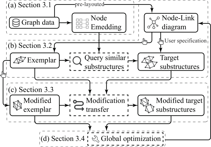
Figure 1: Workflow of our end-to-end system: (a) pre-computing node embeddings and laying-out a node-link diagram; (b) detecting similar target substructures with a specified exemplar; (c) transferring user modifications to similar substructures; (d) merging modified substructures into the entire layout with global optimization.

2.1 Step 1. Node-embedding-based Representations

Our approach uses a node-embedding technique to embed a node into a low-dimensional vector subject to its local topology. For a given exemplar, we employ the node-embedding-based representation to represent and retrieve similar substructures from the entire graph. In this way, we simplify the subgraph-retrieving problem to a similar multidimensional data-searching problem. Though various node-embedding representations [13, 26, 28, 45, 53] are compatible with our approach, we leverage GraphWave [13] following the study conducted in [4]. We pre-compute node embeddings because this process is time-consuming.

2.2 Step 2. Specifying Exemplar and Targets

The user can specify a substructure using the lasso interactions in the node-link diagram (Figure 2a). We then use the similar structure-query technique in [4] to retrieve a set of substructures that are potentially similar to the exemplar (Figure 2c). Four parameters are used in the searching process. The parameter $k$ is used in the $k$-nearest neighbors algorithm for retrieving similar nodes. A large $k$ may introduce many candidate nodes in a huge connected substructure; it will be filtered out by parameter $max$. On the other hand, a small $k$ limits the number of candidate nodes, so that the probability of forming a connected substructure is small. The parameter $k$ should be tuned interactively. We eliminate similar substructures whose node number is less than the minimum count ($min$) or more than the maximum count ($max$). We suggest setting $min$ and $max$ to be close to the number of nodes in the exemplar (e.g., set $min$ to be half $\#nodes$ and $max$ to be twice $\#nodes$), so as to generate substructures of similar scale to the exemplar. We also remove substructures whose Weisfeiler-Lehman similarity is less than the minimum similar threshold ($\epsilon$).

Also, we let the user specify additional structures in the node-link diagram using lasso interactions. We regard both retrieved substructures and user-specified substructures as target substructures.

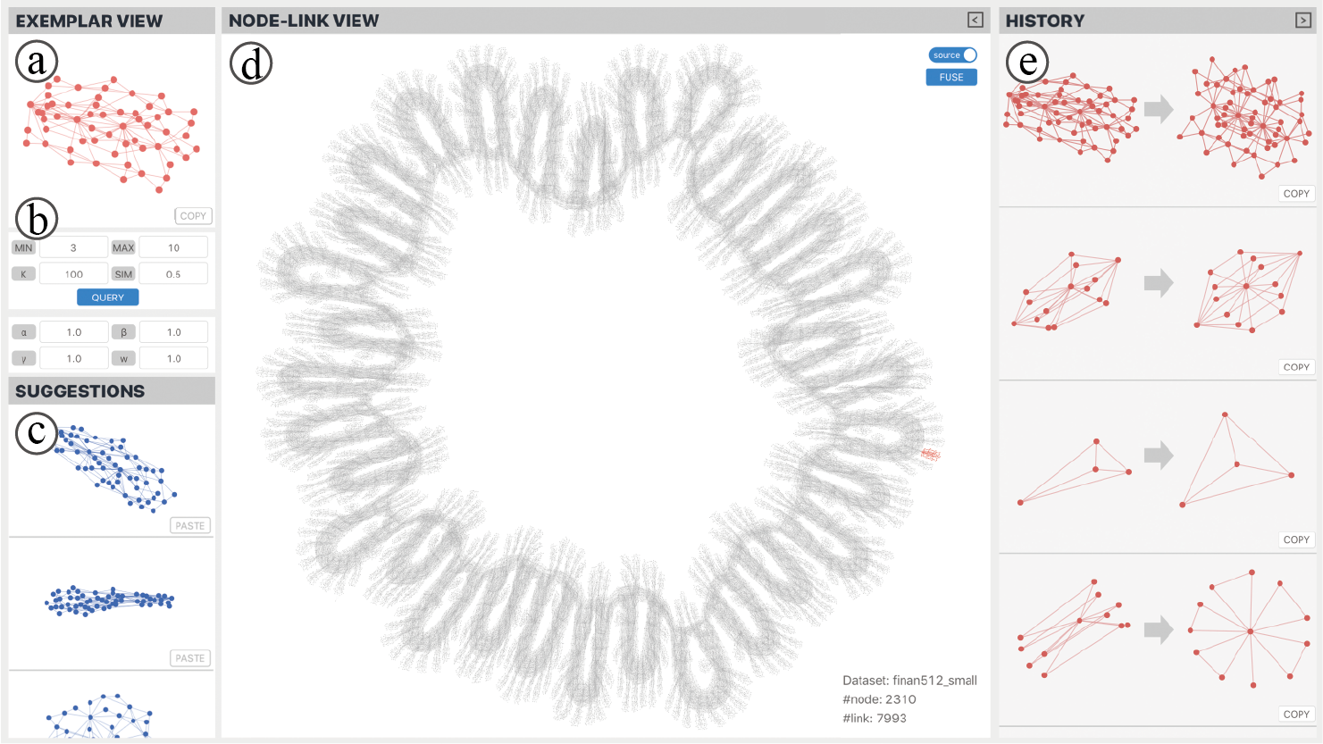
Figure 2: The user interface of our prototype system: (a) an exemplar view; (b) a control panel; (c) a suggestions gallery; (d) a node-link view; (e) a modification history view.

2.3 Step 3. User-driven Fine-tuning

Our approach uses dragging interaction to interactively manipulate the exemplar’s layout. The modification transfer algorithm described in Section 3 can transfer the exemplar’s layout modifications to target substructures’ layouts. We design an interaction mode called “format painter” (inspired by operations in Microsoft Word) to perform the modification transfer. After modifying the exemplar’s layout, the user can transfer modifications to other target substructures using the “copy” and “paste” buttons. Our approach records modifications after the user clicks the “copy” button and transfers modifications into target substructures after the user clicks the “paste” button.

2.4 Step 4. Global Layout Optimization

The exemplar and target substructures are parts of the entire graph. Directly merging the modified layout into the entire graph may lead to abrupt boundaries of the modified substructures (Figure 3b). Thus, we perform a global optimization to preserve the smooth boundaries of the modified substructures (Figure 3c). The optimization process is similar to the deforming step, like the stress-majorization layout [21] (see Section 3.2). We preserve details of the entire graph by minimizing the relative position displacements of each node pair. However, optimizing the entire graph is computationally expensive. We found that deforming the layout of the surroundings of the exemplar and target is to some extent adequate to reach smoothness. The surroundings of a structure are the induced subgraph of the entire graph whose nodes’ distances are less than a given distance $d$ to the structure, where $d$ is the maximum edge length in the entire graph. This ensures that nodes adjacent in both topology and Euclidean distance can be included.

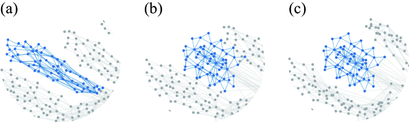
Figure 3: Global optimization in the Finan512 dataset case study; (a) original layout; (b) merging the modified target substructure into entire graph without any optimization; (c) merging modified target with our technique.

2.5 Visual Interface

We design and implement a visual interface, which consists of 4 parts: The exemplar view (Figure 2a) supports exploring and modifying a specified exemplar. When the user finishes modifications, the user can use “format painter” to transfer modifications to the targets. The control panel (Figure 2b) enables the user to adjust parameters of the modification transfer algorithm and the similar-substructure-retrieval algorithm. The suggestion gallery (Figure 2c) sequentially displays similar structures according to their Weisfeiler-Lehman similarities to the exemplar in node-link diagrams. In the meantime, the user can specify a structure in the node-link diagram as a suggestion; this is displayed at the top of the suggestion gallery. The node-link view (Figure 2d) provides visualizations with various graph-layout algorithms. The user can use the lasso to specify a substructure as an exemplar, which the exemplar view will then display. The modification history view (Figure 2e) records layout change history applied to the exemplar. Each record relates to a piece of modification on the exemplar. The layouts before and after modifications are shown side by side. The user can reuse modifications in the history view for transferring. The most recent history is displayed at the top.

3 Modification Transfer in Graph Structures

Here we introduce a modification-transfer algorithm to transfer layout adjustments from one graph structure to another. We define terms in Table 1. Here, given a source graph structure layout $S=(V^{s},E^{s})$, user modifications change $S$ into a new layout $S^{\prime}$. And given a target graph structure layout $T=(V^{t},E^{t})$, we denote the modification transfer as a process of analogizing the modifications ($S\rightarrow S^{\prime}$) to the target graph ($T\rightarrow\tilde{T}^{\prime}$) in three steps:

1. Marker selection first aligns $T$ and $S$ with correspondences $C$ generated by the graph-matching method and then selects some finely matched correspondences as markers (Figure 4a).

2. Layout simulation ($T\stackrel{{\scriptstyle S}}{{\longrightarrow}}\tilde{T}$) alters the layout of the target from $T$ to $\tilde{T}$ to simulate $S$ and expands $M$ to $\tilde{M}$ (Figure 4b).

3. Layout simulation ($\tilde{T}\stackrel{{\scriptstyle S^{\prime}}}{{\longrightarrow}}\tilde{T}^{\prime}$) alters the layout of the target from $\tilde{T}$ to $\tilde{T}^{\prime}$ to simulate $S^{\prime}$ (Figure 4c).

Here, we perform two rounds of layout simulate because $S^{\prime}$ is usually different from $T$, directly deforming $T$ into the shape of $S^{\prime}$ can lead to unpleasing transfers.

Table 1: Definition of symbols. Here $G=(V,E)$ denotes a graph with its layout, where $V=\left\{v_{1},v_{2},\ldots,v_{n}\right\},v_{i}\in\mathbb{R}^{2}$ contains the positions of a set of $n$ nodes and $E=\left\{e_{1},e_{2},\ldots,e_{m}\right\}$ is a set of $m$ edges in $G$.

Symbol	Description
$S=(V^{s},E^{s})$	A source graph layout
$S^{\prime}$	A modified source graph layout
$T=(V^{t},E^{t})$	A target graph layout
$\tilde{T}=(\tilde{V}^{t},E^{t})$	The target graph layout that simulates $S$’s layout
$\tilde{T}^{\prime}$	The target graph layout that simulates $S^{\prime}$’s layout
$M$	The set of paired markers that matches $V^{s}$ to $V^{t}$
$(m^{s}_{i},m^{t}_{i})\in M$	A pair of markers where $m^{s}_{i}\in V^{s}$ and $m^{t}_{i}\in V^{t}$
$C$	Correspondences between $S$ and $T$
$(c^{s}_{i},c^{t}_{i})\in C$	A correspondence pair where $c^{s}_{i}\in V^{s}$ and $c^{t}_{i}\in V^{t}$
$(v_{i}[x],v_{i}[y])$	The $x$ and $y$ positions of node $i$
$V(k)$	Positions of the node set $V$ in the iteration $k$
$\mathbf{R}$	A $3\times 3$ affine transformation matrix

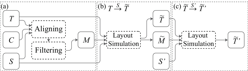
Figure 4: Modification transfer. (a) Marker selection: aligning layouts of target $T$ and source $S$ first, and then selecting a set of markers $M$ from given correspondences $C$ between $S$ and $T$; (b) the first round of layout simulation: altering the layout $T$ to simulate $S$, which produces a new target structure layout $\tilde{T}$ and expands $M$ to $\tilde{M}$; (c) the second round of layout simulation: altering the layout $\tilde{T}$ to simulate $S^{\prime}$, which produces $\tilde{T}^{\prime}$.

3.1 Marker Selection

The modification transfer algorithm relies on the correspondences between two structures, denoted as $C=\{(c^{s}_{i},c^{t}_{i})\},1\leq i\leq\min(|V^{s}|,|V^{t}|)$. Any graph-matching method that produces injective correspondences is suitable for modification transfer. Six graph-matching methods [7, 9, 25, 42, 67, 68] are examined (see Suppl. Material and Section 4.1 for comparison details). We employ Factorized Graph Matching (FGMU) [68] because it achieves the best efficiency.

Because graph-matching methods may depend on the graph layout, we layout the exemplar and target substructures with the same algorithm before constructing correspondences. We employ FM³ [27] because it is one of the most efficient layout algorithms to our knowledge. The graph-matching methods can generate unpleasant matching results because these methods build correspondences for all nodes even if they are not well matched. To examine their correspondences, we first align two graph structures $S$ and $T$ according to the correspondences (described in Section 3.2). If the graph-matching method generates correct correspondences, we align two corresponding nodes together in the aligning step and almost all of their neighborhoods can possibly be matched. Thus, we implement the correspondences filtering algorithm (Algorithm 1) to select “fine” correspondences ($(c^{s}_{i},c^{t}_{i})$) that satisfy:

1. The distance between $c^{s}_{i}$ and $c^{t}_{i}$ is less than the average length of their adjacent edges multiplied by a given ratio ($r_{d}$); and

2. $c^{s}_{i}$’s neighbors are mostly matched to $c^{t}_{i}$’s neighbors (with a ratio greater than $r_{u}$).

We fix $r_{d}$ and $r_{u}$ to be $2$ and $0.5$ in our implementation. A smaller $r_{d}$ and a larger $r_{u}$ lead to fewer, possibly more accurate correspondences. There is a trade-off between accuracy and number of correspondences. Here, we use these “fine” correspondences as a set of markers $M$ for the layout simulation. In addition, our approach also supports specifying markers manually to match user preferences. The user can click on two nodes, one in each of the exemplar and target substructures, to specify a pair of markers.

Algorithm 1 Correspondences filtering

1:$S=(V^{s},E^{s})$: a source graph; $T=(V^{t},E^{t})$: a target graph; $C=\left\{(c^{s}_{i},c^{t}_{i})\right\}$: a set of correspondences; $r_{u}$: a minimum common neighbors ratio; $r_{d}$: a maximum distance ratio;

2:$M=\left\{(m^{s}_{i},m^{t}_{i})\right\}$: a set of markers;

3:Init markers $M=\varnothing$

4:for each correspondence pair $(c^{s}_{i},c^{t}_{i})$ do

5:     $ns\leftarrow c^{s}_{i}$’s neighbors’ corresponding nodes

6:     $nt\leftarrow c^{t}_{i}$’s neighbors

7:     $nu\leftarrow ns\bigcap nt$

8:     if $Count(nu)>Count(ns)\times r_{u}$ or $Count(nu)>Count(nt)\times r_{u}$ then

9:         $ds\leftarrow$ the mean length of adjacent edges of $c^{s}_{i}$

10:         $dt\leftarrow$ the mean length of adjacent edges of $c^{t}_{i}$

11:         $d\leftarrow$ distance between $c^{s}_{i}$ and $c^{t}_{i}$

12:         if $d<ds\times r_{d}$ and $d<dt\times r_{d}$ then

13:              Add $(c^{s}_{i},c^{t}_{i})$ into $M$

14:         end if

15:     end if

16:end for

17:return $M$;

3.2 Layout Simulation

The goal of the layout simulation is to smoothly deform the markers of the target $T$ to those of the source $S$, while preserving the original layout of the target $T$ as much as possible (Figure 5). We do this in three steps: aligning, deforming, and matching. The aligning step scales, rotates, and translates $T$ to minimize the dissimilarity to $S$ (Figure 5d). The deforming step alters the node positions of $T$ to simulate the shape of $S$ (Figure 5e). The matching step constructs correspondences between the nodes of $T$ and $S$ by searching their neighbors (Figure 5f). These steps iteratively deform $T$ into the shape of $S$ until no more new correspondences are constructed.

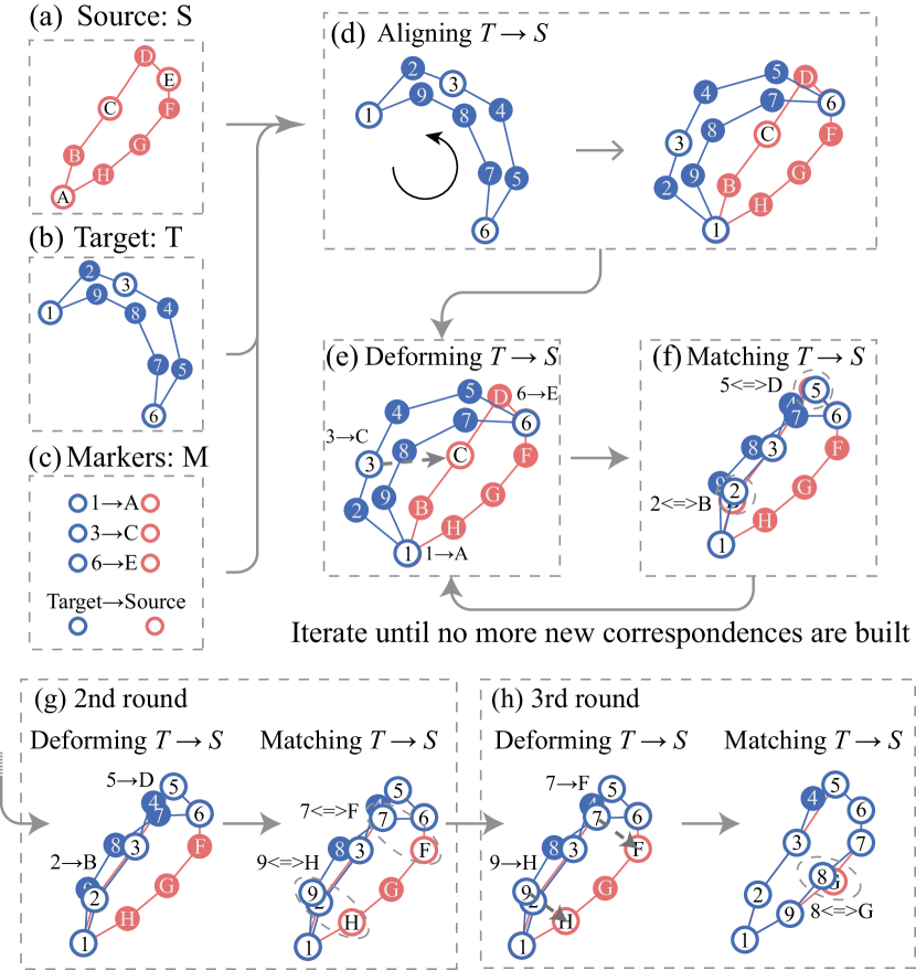
Figure 5: Layout simulation: altering the shape of a target structure $T$ to simulate the layout of a source structure $S$. (a) a source structure $S$; (b) a target structure $T$; (c) a set of markers $M$; (d) aligning $T$ to $S$ with markers $M$; (e) deforming $T$ into $S$ with markers $M$; (f) matching the nodes of $T$ to the nodes of $S$; two pairs of markers are constructed: {(2,B) and (5,D)}; (g) the second round of deforming and matching; two marker pairs are constructed: {(7,F) and (9,H)}; (h) the third round of deforming and matching, one pair of markers is constructed: {(8,G)}; Iterations are performed until no more new correspondences are built.

Aligning. We assume that both the topology and the layout of the source structure are similar to the target. To minimize the layout difference, the node-link diagrams of $S$ and $T$ are aligned. This step only transforms the global location and orientation of the target structure, not the positions of individual nodes.

We use a small set of predefined markers to achieve an optimal alignment. The markers are a set of paired nodes $M=\left\{(m^{s}_{i},m^{t}_{i})\right\},m^{s}_{i}\in V^{s},m^{t}_{i}\in V^{t}$ (Figure 5c). The markers on the source and the target are aligned by an affine transformation $\mathbf{R}$:

$$\mathbf{R}=scale\times\left(\begin{array}[]{ccc}\cos\theta&\sin\theta&tx\\ -\sin\theta&\cos\theta&ty\\ 0&0&1\end{array}\right)\approx\left(\begin{array}[]{ccc}s&h&tx\\ -h&s&ty\\ 0&0&1\end{array}\right)$$ (1)

where $scale$ is the scale coefficient, $\theta$ is the rotation angle, and $tx$ and $ty$ are the translation components. For the sake of simplicity, we use a linear approximation of $\mathbf{R}$ (after the approximately equal sign). $\mathbf{R}$ is calculated by solving the minimization problem:

$$\min_{\mathbf{R}}\sum_{i}^{|M|}||\mathbf{R}m^{t}_{i}-m^{s}_{i}||^{2},$$ (2)

where $(m^{t}_{i},m^{s}_{i})\in M$ denotes one pair of markers. The minimization problem is equivalent to the problem:

$$\min_{\mathbf{T}}\sum_{M}||\mathbf{A}(s,h,tx,ty)^{T}-\mathbf{b}||^{2},$$ (3)

where $\mathbf{A}$ contains the positions of the markers in the target and $\mathbf{b}$ contains the positions of the markers in the source:

$$\mathbf{A}=\left(\begin{array}[]{llll}{m^{t}_{i}}[x]&{m^{t}_{i}}[y]&1&0\\ {m^{t}_{i}}[y]&-{m^{t}_{i}}[x]&0&1\\ \vdots\end{array}\right),\mathbf{b}=\left(\begin{array}[]{c}{m^{s}_{i}}[x]\\ {m^{s}_{i}}[y]\\ \vdots\end{array}\right),i=1,\ldots,|M|.$$ (4)

${m^{t}_{i}}[x]$ and ${m^{t}_{i}}[y]$ are the positions of the target marker $m^{t}_{i}$ and ${m^{s}_{i}}[x]$ and ${m^{s}_{i}}[y]$ are the positions of the source marker $m^{s}_{i}$. The minimization problem can be solved by:

$$(s,h,tx,ty)^{T}=\mathbf{A}^{\dagger}\mathbf{b},$$ (5)

where $\mathbf{A}^{\dagger}$ is the Moore-Penrose pseudoinverse [48] of $\mathbf{A}$. Thus, the transformation can be defined as a linear function of the markers in the source. With the affine transformation matrix $\mathbf{R}$, $T$ is transformed to align $S$ by a linear transformation (Figure 5d). After modification transfer, the target layout is restored by an inverse process of the alignment step, so that it can be merged into the entire layout with the original rotation and scale.

Deforming. The deforming step seeks to alter the shape of $T$ to simulate $S$. We design an energy function to represent the process:

$$E=E_{S}+\gamma E_{M},$$ (6)

where $\gamma$ is a weight parameter. The deforming step is equivalent to minimizing $E$. It seeks to force positions of target markers $m^{t}_{i}$ to approach source markers $m^{s}_{i}$ ($E_{M}$) while preserving the original layout information to reach a smooth deformation ($E_{S}$). Here, we denote $E_{M}$ as the sum of distances between pairs of markers:

$$E_{M}=\sum_{i}^{|M|}||{m^{t}_{i}}-{m^{s}_{i}}||^{2}.$$ (7)

$E_{S}$ represents the layout change between $T$ and $\tilde{T}$, which is constructed by two items:

$$E_{S}=\alpha E_{O}+\beta E_{D},$$ (8)

where $\alpha$ and $\beta$ are two weights, $E_{O}$ is designed to preserve orientations of vectors between node pairs after the aligning step, and $E_{D}$ is designed to preserve distances between node pairs. $E_{O}$ is defined as:

$$E_{O}=\sum_{i<j}w_{ij}||norm(v^{t}_{i}-v^{t}_{j})-norm(\tilde{v}^{t}_{i}-\tilde{v}^{t}_{j})||^{2}.$$ (9)

Here, $norm(\cdot)$ denotes the normalization of a vector. $E_{D}$ is defined as:

$$E_{D}=\sum_{i<j}w_{ij}(||v^{t}_{i}-v^{t}_{j}||-||\tilde{v}^{t}_{i}-\tilde{v}^{t}_{j}||)^{2},$$ (10)

where $w_{ij}$ is the weight related to the node pair $(v^{t}_{i},v^{t}_{j})$, and $(\tilde{v}^{t}_{i},\tilde{v}^{t}_{j})$ is a node pair of the target structure after deformation ($\tilde{T}$). $w_{ij}$ is defined as:

$$w_{ij}=\left\{\begin{array}[]{ll}w||v^{t}_{i}-v^{t}_{j}||^{-2},&\text{ if }\left\{i,j\right\}\in E^{t}\\ ||v^{t}_{i}-v^{t}_{j}||^{-2},&\text{ otherwise }\end{array}\right.,$$ (11)

where $w$ is a preservation degree on the edges. Setting $w$ greater than $1$ makes the algorithm pay more attention to preserve orientations and length of edges.

Preferences on preservation of distances and orientations can be configured by balancing $\alpha$ and $\beta$. For example, when $\alpha$ is small, the distances between node pairs can be mostly preserved (Figure 6b). If we enlarge $\alpha$, the orientations can be better preserved (Figure 6c). Both weighting schemes are optional. The parameter $\gamma$ is used to configure the weight of moving marker positions in the target structure to their counterparts. A large $\gamma$ ensures that markers of $S$ and $T$ can be aligned.

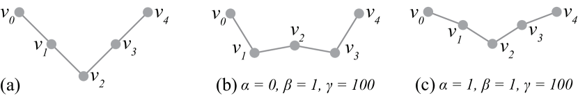
Figure 6: Different weighting schemes. The node $v_{2}$ is moved to a higher position while nodes $v_{0}$ and $v_{4}$ are fixed in their original positions. (a) is the original layout. (b) is the layout that preserves the distances with $\alpha=0,\beta=1$, and $\gamma=100$. (c) is the layout that keeps both orientations and distances with $\alpha=1,\beta=1$, and $\gamma=100$.

Following the optimization process in the stress majorization technique [21], $E_{O}$ and $E_{D}$ can be minimized by iteratively solving:

$$L_{w}^{V^{t}(k)}V^{t}(k+1)=L_{w}^{V^{t}}V^{t},$$ (12)

and

$$L_{w}V^{t}(k+1)=L_{w}^{V^{t}(k)}V^{t}(k),$$ (13)

where $V^{t}(k)$ and $V^{t}(k+1)$ are the target nodes in time $k$ and $k+1$. $L_{w}$ and $L_{w}^{V^{t}}$ are two weighted Laplacian matrices defined as:

$$(L_{w}^{V^{t}})_{ij} =\left\{\begin{array}[]{ll}-w_{ij}inv(||V^{t}_{i}-V^{t}_{j}||),&i\neq j\\ \sum_{l\neq i}(L_{w}^{V^{t}})_{il},&i=j\\ \end{array}\right.$$ (14)

$$(L_{w})_{ij} =\left\{\begin{array}[]{ll}-w_{ij},&i\neq j\\ \sum_{l\neq i}w_{il},&i=j\\ \end{array}\right.,$$

and the definition of $L_{w}^{V^{t}(k)}$ is similar to $L_{w}^{V^{t}}$ except that $v^{t}_{i}$ and $v^{t}_{j}$ are replaced by their counterparts in time $k$. The process is repeated until the target layout stabilizes.

Matching. The matching step constructs node correspondences between $S$ and $T$. Any node pair $(v^{s}_{i},\tilde{v}^{t}_{j}),i\leq|V^{s}|,j\leq|\tilde{V}^{t}|$ that satisfies $||v^{s}_{i}-\tilde{v}^{t}_{j}||<r_{j}$ is identified as one candidate correspondence. We consider that $r_{j}$ should be adaptive to different $\tilde{v}^{t}_{j}$, and thus, we associate $r_{j}$ to the mean length of $\tilde{v}^{t}_{j}$’s adjacent edges. By default, $r_{j}$ is set to be twice the mean length of the adjacent edges to avoid filtering out too many candidate node pairs. To avoid overlapping, correspondences should be injective. This maximum assignment problem can be solved by the Hungarian algorithm [39, 40]. Here, we use distances between node pairs as the cost in the Hungarian algorithm.

Adequate correspondences can yield accurate modification transfer. Thus, the aligning, deforming, and matching steps are iteratively performed by using the already-built correspondences or markers. For example, Figures 5(e-f) show the first round of deformation. With three markers, the target can not faithfully mimic the shape of the source. Additional correspondences are constructed by searching neighbors (Figure 5f). Two more deforming and matching rounds improve the accuracy (Figures 5(g-h)). The iteration stops until the number of correspondences no longer increases. $\tilde{T}$ is often similar to $S$ after deformation (Figure 5h). After that, layout simulation is performed again to alter the deformed target $\tilde{T}$ into the modified source $S^{\prime}$ (Figure 4c).

4 Results and Evaluation

We implement our system in a browser-based architecture. The front-end application is developed with JavaScript using React and D3. The back-end server uses Python 3.7.5 with flask, networkx, numpy, and scipy. All experiments are performed on a Macbook Pro laptop with an Intel Core i7-7820HQ CPU (2.9 GHz) and 16 GiB RAM.

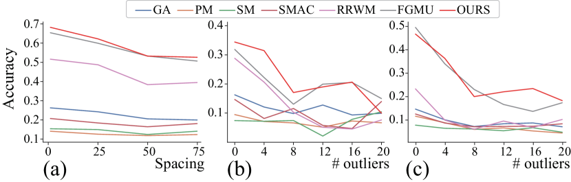
Figure 7: Quantitative comparison of several conventional graph matching methods and our approach: (a) average accuracy of different frame spacing in the CMU-house-image dataset; (b) average accuracy of different numbers of outliers in the Motorbike-image dataset; (c) average accuracy of different numbers of outliers in the Car-image dataset.

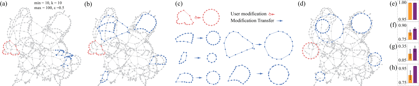
Figure 8: Case study with Power-Network dataset [54]: (a) an exemplar (in red) and two retrieved substructures (in blue, which are overlapped) overlaid on a network depicted using FM³ [27]. (b) Two retrieved substructures are discarded. And several target substructures are specified manually.(c) The shape of the exemplar is changed to a circle. Modification transfer alters the node positions of targets to simulate the exemplar’s shape. (d) All modified substructures are merged into the graph by an automatic optimization. (e-h) Readability before (orange) and after (purple) modification transfer measured by four readability criteria (from top to bottom: crosslessness, minimum-angle metric, edge-length variant, and shape-based metric);; error bars depict 95% confidence intervals.

4.1 Quantitative Comparison

Our approach uses a set of markers generated by graph-matching methods for modification transfer. We compared conventional graph-matching methods to ours using the following benchmark datasets with manually labeled ground truth:

1. The CMU-house-image dataset [68] contains 111 frames of a house with 30 landmarks. We randomly remove 5 landmarks and generate a graph with Delaunay triangulation that connects landmarks for each frame. Frames are paired spaced by 0, 25, 50, and 75 frames, yielding 444 pairs.

2. The Car-and-Motorbike image dataset [43] has 30 pairs of car images and 20 pairs of motorbike images. We used Delaunay triangulation to generate graphs for each image, added 0, 4, 8, 12, 16, and 20 outliers randomly, and removed unconnected nodes, yielding 222 pairs of graphs.

Node-link diagrams of these datasets are generated by the well-studied force-directed layout algorithm. We compare the accuracy of graph matching results. Figure 7 shows the average matching accuracy on different datasets. Our approach works slightly better than FGMU and exceeds other methods, meaning that our improvements on FGMU can generate more accurate results in most cases. Note that graphs in these benchmark datasets are smaller than those in the case studies.

4.2 Case Studies

We show how our exemplar-based layout fine-tuning approach works in three case studies.

We used FM³ [27] to generate the layout of the Finan512 dataset from the University of Florida Sparse Matrix Collection [11], which is generated from multistage stochastic financial modeling [57]. The graph consisted of 74,752 nodes and 261,120 edges rendered in WebGL (Figure Exemplar-based Layout Fine-tuning for Node-link Diagramsa). We saw several “donut-like” substructures.

Next, we specified a substructure (here called an exemplar) for fine-tuning (Figure Exemplar-based Layout Fine-tuning for Node-link Diagramsb). We retrieved similar substructures using $k=200$, $min=10$, $max=100$, and $\epsilon=0.95$ (Figure Exemplar-based Layout Fine-tuning for Node-link Diagramsa). To verify the topology of these substructures, we select target substructures as the five most similar and five most dissimilar substructures according to their Weisfeiler-Lehman similarities to the exemplar (Figure Exemplar-based Layout Fine-tuning for Node-link Diagramsc). In addition, to fine-tune the “donut” subgraph, we use substructures around it as target substructures.

We interactively modified the exemplar into a layout with a distinguishable structure (Figure Exemplar-based Layout Fine-tuning for Node-link Diagramse). After modification transfer, these substructures became clearer (Figures Exemplar-based Layout Fine-tuning for Node-link Diagrams(f, g)).

Our smooth merging scheme generated visually pleasing details compared to direct merging without any optimization. For example, the boundary of the substructure in Figure 3c is easier to distinguish than the one without optimization in Figure 3b.

The Power-Network dataset is collected from the Network Data Repository [54], which abstracts a power system: the nodes encode buses and edges are the transmission lines among the nodes. The network contains 662 nodes and 906 edges. A multilevel graph layout implemented by Tulip [1] and OGDF [6] is employed to layout the network (Figure 8a).

To reveal transmissions among a set of buses that may form a cycle, we specify a set of nodes as an exemplar (Figure 8a, in red). With $min=10$, $max=100$, $k=5$, and $\epsilon=0.5$, two overlapped structures are retrieved (Figure 8a, in blue). The retrieved structures are not topologically similar to the exemplar, because our technique detects embedding-similar structures, which are potentially similar to the exemplar. Thus we explore the node-link diagram to specify target substructures. Several sets of nodes that may form cycles are specified as target substructures (Figure 8b, in blue). Connections among these nodes are obscured by the visual clutter. The exemplar is interactively modified into a circle. Each target is deformed into a circle-like shape by transferring modifications (Figure 8c). Now the connections among nodes are far more distinguishable (Figure 8d) than the original layout.

We increase $\alpha$ to increase the degree of orientation preservation, which means that orientations of edges tend to remain unchanged. This makes the shape of the modified target substructure smoother (Figure 9c). Because the edge lengths before modification transfer are not identical (Figure 9a), solely preserving distances can lead to unsatisfying deformations. For example, setting $\alpha$ in Equation 8 to be zero generates irregular polygons (Figure 9b).

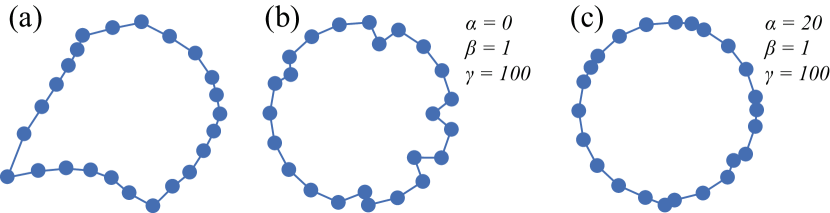
Figure 9: Different weighting schemes for the Power-Network dataset. (a) a target substructure; (b) a low preservation on orientations with $\alpha=0$, $\beta=1$, and $\gamma=100$; (c) a large preservation on orientations with $\alpha=20$, $\beta=1$, and $\gamma=100$.

The Price_1000 dataset is a tree from tsNET [37] that consists of 1000 nodes and 999 edges. We layout the graph with a simple radial tree layout algorithm [33] (Figure 10a), and find that sibling nodes are overlapped due to the space constraint.

We select one representative subtree as an exemplar. To reduce visual clutter,this is reconfigured into a radial tree layout (Figure 10b). To reconfigure other interested subtrees, we specify two nodes of the exemplar as markers, and the algorithm transfers modifications on the exemplar to other subtrees (Figure 10c).

Although there are some unpleasing details, their layouts are similar to the exemplar’s. Rather than interactively reconfiguring these subtrees from the original layout, our approach requires only a few slight modifications according to the minimum angle and the symmetry aesthetic metrics [52] to tune the details (Figure 10d) because it generates an initial layout for each subtree.

Readability. To evaluate the readability of the results generated by our approach, we use the measurements (crosslessness, minimum-angle metric, edge-length variation, and shape-based metric) in [41] to test readability improvement. All these measurements are normalized. Larger values of the measurements suggest higher readability except edge-length variation. Results of readability measurements for the Finan512 dataset, the Power-Network dataset and the Price_1000 dataset are given in Figures Exemplar-based Layout Fine-tuning for Node-link Diagrams(h,i,j,k), Figures 8(e,f,g,h), Figures 10(e,f,g,h), accordingly. Bars representing measurement values before modification transfer are in orange and bars after modification transfer are in purple. Note that, in the case study with the Price_1000 dataset, we also measure the readability after slight modifications (in light purple). Results show that our approach improves readability in most cases.

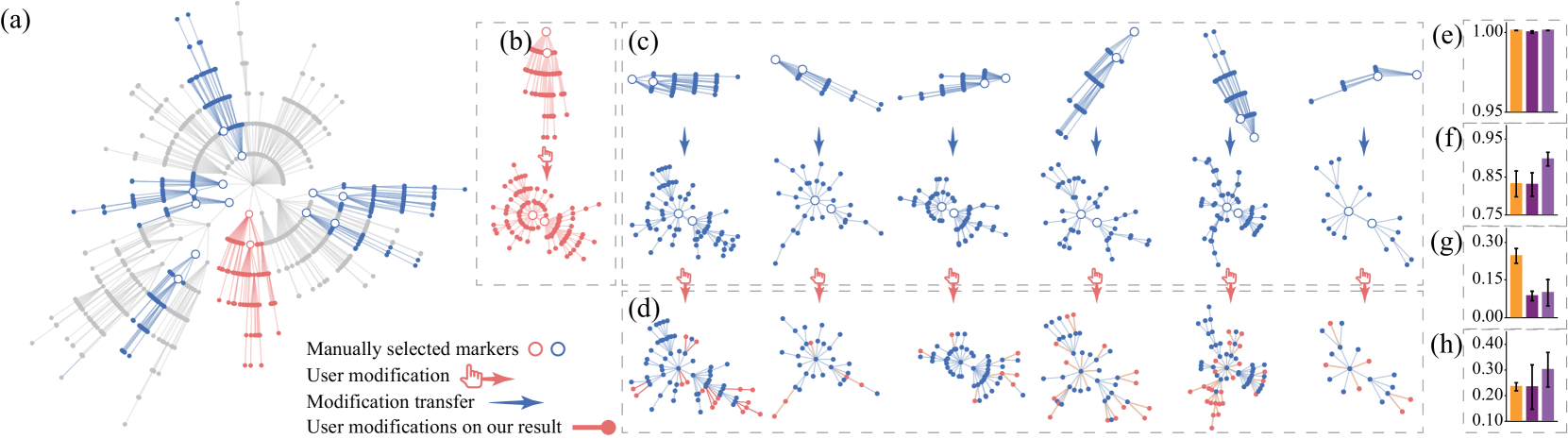
Figure 10: The Price_1000 dataset [37]. (a) A radial tree layout. (b) A specified exemplar in which we specify two nodes with the two largest degrees as markers. This is modified into a radial tree layout interactively. (c) Targets and their counterparts after modification transfer. (d) Modified targets after several slight user modifications (in red). (e-h) Readability before (orange) and after (purple) modification transfer measured by four readability criteria (from top to bottom: crosslessness, minimum-angle metric, edge-length variant, and shape-based metric); error bars depict 95% confidence intervals..

4.3 User Study

We conducted a within-participant experiment in which we asked participants to fine-tune structures’ layouts in three modes:

1) Baseline manual: mouse dragging without our approach;

2) Our semi-automatic method with markers specified by user;

3) Our fully automatic method with markers initialized by filtering the results of FGMU.

Task. Participants performed a task involving modifying the structure on the screen according to the expert’s modifications on the exemplar. Twenty substructures from four real-world datasets are used.

Datasets. A graph visualization expert helped us define the 20 total substructures used in the study. He first chose five exemplar substructures from four real-world datasets and then specified three target structures for each of the five exemplars (Figure 11). Graphs generated from four real-world datasets have already been laid out with FM³ [27]. Substructures are extracted with node positions. The expert was also asked to modify five exemplars’ layouts to support our task.

1) The Email-Eu-core dataset [51] is a time-varying email contact network in a large European research institution with 986 nodes and 332,334 contacts. Email communications within every 24 hours form a graph, yielding a total of 803 snapshots with 855 connected subgraphs. We obtained the first exemplar and its three target structures from Email-Eu-core dataset (Figure 11a). The expert modified the exemplar into a fan-like shape (Figure 11a-1).

2) The Mouse-Brain dataset [18] consists of 986 nodes and 1,536 edges. Nodes represent the mouse visual cortical neurons and edges are fiber tracts connecting one neuron to another. We obtained the second exemplar and its three target structures from the Mouse-Brain dataset (Figure 11b). The expert modified the exemplar into a star-like shape in which the interior node stays in the center and the leaves are placed evenly around the interior (Figure 11b-1).

3) The Euroroad dataset [58] is a road network mostly in Europe. Nodes represent cities and an edge between two nodes denote that they are connected. The network consists of 1,174 nodes and 1,417 edges. We obtained the third exemplar and its three target structures (Figure 11c) are extracted from the Euroroad dataset [58]. The expert modified the exemplar into a round circle (Figure 11c-1).

4) The High-School-contact dataset collected from the SocioPatterns initiative [47] consists of 180 nodes and 45,047 contacts. We created a temporal network following the procedure in [60]. The last two exemplars and six target structures were obtained from the High-School-contact dataset (Figures 11(d, e)). The expert modified one exemplar into a shape in which the inner circle is laid out as a regular polygon and the surrounding nodes are placed orthogonally (Figure 11d-1). And he modified the other exemplar into an orthogonal layout (Figure 11e-1).

We ensured that within the same dataset, the Weisfeiler-Lehman similarities between three target substructures and the exemplar are greater than 0.7. We recorded all modifications made by the expert along with a list of instructions (see Suppl. Material).

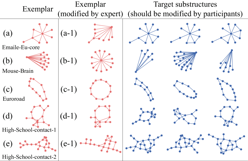
Figure 11: Data samples in the user study. Five exemplars and 15 target substructures were extracted from the four datasets. (a) is extracted from the Email-Eu-core dataset [51]; (b) is from the Mouse-Brain dataset [18]; (c) is from the Euroroad dataset [58]; (d) and (e) are from the High-School-contact dataset [47].

Participants and apparatus. Twelve volunteers were recruited to participate in the study (5 males, 7 females; aging from 23 to 27). All participants were students or researchers concentrating in computer science. They are familiar with visualization and four of them major in graph visualization. The study was conducted on a PC provided by us equipped with a mouse, keyboard, and 24-inch display. The interface was displayed within a window size of 1920 $\times$ 1080 resolution. Parameters of the modification transfer are fixed to $\alpha=1,\beta=5,\gamma=1000,\text{ and }w=1$.

Study Conditions. We tested the performance of different fine-tuning techniques (baseline manual, semi-automatic, and fully automatic) on a small graph layout. Each participant was asked to process three target structures in all four cases (one from the Mouse-Brain dataset, one from the Euroroad dataset, and two from the High-School-contact dataset) with three techniques, yielding 432 ($12\text{ participants}\times 4\text{ cases}\times 3\text{ targets}\times 3\text{ techniques}$) trials.

Procedure. The study has two stages. We first trained participants on the three manipulation modes (baseline manual, semi-automatic, and fully automatic). They viewed a demo video of an expert’s operations using data samples extracted from the Email-Eu-core dataset (Figure 11a), and then practiced till they felt comfortable with the tasks. In the formal study, they were then asked to manipulate three targets’ shapes to simulate the exemplar for each case using all three techniques ($4\text{ cases }\times 3\text{ targets }\times 3\text{ techniques }$ in total for each participant). For each trial, an exemplar, a modified exemplar, and a target substructure were displayed on the interface (see Suppl. Material). Participants were asked to manipulate the target substructure to simulate modifications made on the exemplar by comparing the exemplar and the modified exemplar. They could also follow printed instructions (see Suppl. Material). With our semi-automatic method, participants were asked to specify markers first. One pair of markers was constructed by clicking on two nodes, one from the exemplar and one from the target substructure. With our fully automatic method, markers were constructed automatically. Our two methods produced initial layouts that simulate the expert’s modifications and participants were asked to perform the task based on initial layouts. Parameters and initial layouts were the same for all participants. The order of four cases, three techniques, and three targets was randomly assigned to each participant to counterbalance learning effects. After the study, participants were interviewed to give some suggestions on our approach.

Hypotheses. We measure performance by participants’ completion time and number of interactions. We anticipate that the quality of the modified exemplar and the targets’ layouts makes little difference because participants were asked to fine-tune the target layouts until they were satisfied. We formulated three hypotheses:

1. Our fully automatic method is more efficient than the baseline manual method.

2. Our semi-automatic method is more efficient than the baseline manual method.

3. There is no difference in performance between our semi-automatic method and our fully automatic method.

Results. Participants spent about 45 minutes on average on the user study and got a reward of around $5 on completion. We recorded the number of interactions (mouse clicking and dragging) that participants performed and completion times to reach a satisfying layout. The completion time includes marker specification, algorithm computation, and layout modification; and the number of interactions includes marker specification and layout modification. Figures 12(a, b) summarizes the results. We analyzed our results using significance tests with significance levels set to $.05$.

The Shapiro-Wilk test, used to test the normality, suggested that both the number of interactions and the completion time did not follow normal distributions. Thus we used the Friedman test and pairwise Wilcoxon test. The Friedman test detected significant differences in both the number of interactions ($\chi^{2}(2)=154.96,p<0.05$) and the completion time ($\chi^{2}(2)=154.625,p<0.05$). Paired Wilcoxon tests were performed on all cases to compare the efficiency among three techniques. There were significant differences among all combinations of three techniques (baseline manual, semi-automatic, and fully automatic) on two measurements (the number of interactions and the completion time). The post-hoc analysis (Figures 12(a, b)) showed that our semi-automatic method performed most efficiently in both two measurements, followed by the baseline method and last our semi-automatic method. Thus H1 held while H2 and H3 were rejected.

Feedback. We collected some representative participant feedback. Most of them made comments along the lines of, “In fully automatic mode, most results are pretty close to exemplar’s results. I have to make little effort to modify them, especially in complex cases. But I still have to verify whether there is room for improvement”. Many of them mentioned that they were encouraged to attempt higher quality by the high-quality result generated by the fully automatic method. Some of them mentioned that “It is boring to wait for the fully automatic method to calculate the result”. Another complaint about our methods is that markers are hard to determine. Most participants had little experience in graph visualization. Interestingly, several participants mentioned that “The user study is like a game, fine-tuning layouts makes me feel relaxed because I generate nice-looking results”. One of them suggested expanding our user study into an online system to collect more user data.

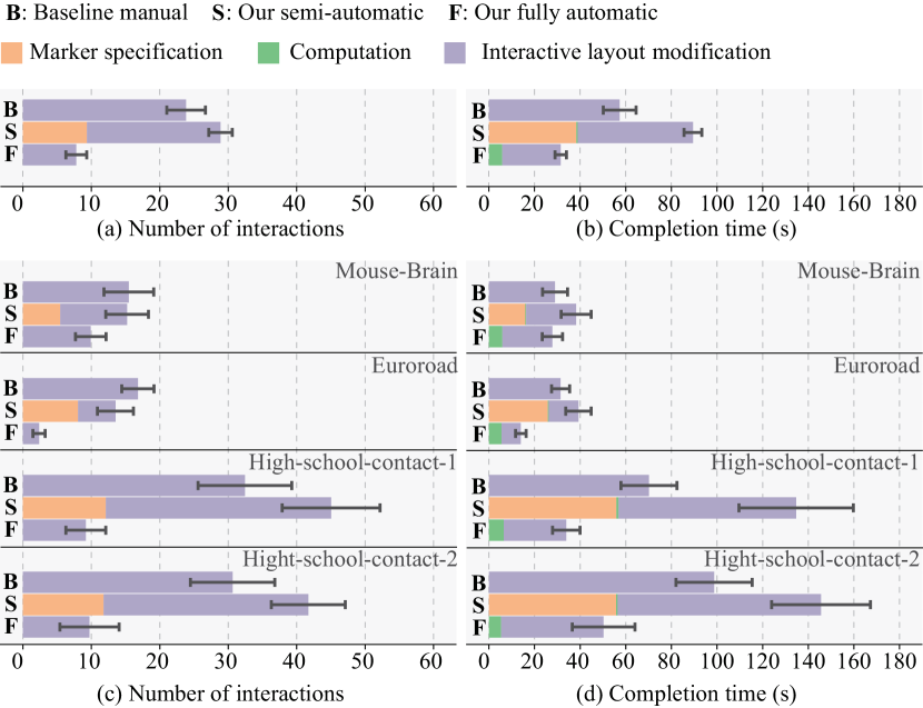
Figure 12: User study results. Measurement components are represented as stacked bars. (a) The distribution of the number of interactions; (b) the distribution of completion time; (c) the distribution of number of interactions on different cases; (d) the distribution of completion time on different cases. Error bars depict 95% CIs.

Discussion. We split the number of interactions and the completion time to look for deeper insights. The completion time consists of three parts: marker specification, algorithm computation, and interactive layout modification (Figure 12d). The computation time occupies a small fraction (in green) in both the semi-automatic and fully automatic methods. The marker specification (in orange) contributes a lot to the completion time of our semi-automatic method. In most cases, participants spent most time on interactively modifying layouts. We also calculated average completion time per interaction for the three methods; participants spent an average of 2.4 second, 2.6 second, and 3.3 second on each layout modifying interaction using the baseline method, our semi-automatic method, and our fully automatic method, respectively. Participants spent more time thinking about and verifying results generated by our fully automatic method. Each interaction for marker specification takes an average of 4.1 seconds. We observe that almost all participants tended to choose internal nodes in the star-like structures (Figure 11b) as markers. However, for structures extracted from the High-School-contact dataset, markers were diverse among participants. We report results of specified markers by an expert on graph analysis in the Suppl. Material. A good pair of markers should be able to assume the same role or status in the source and the target (e.g., cut nodes). This indicates that experience in and knowledge of graph analysis are necessary for marker specifications.

5 Discussion and Limitations

In terms of the performance of modification transfer, our algorithm outperforms the baseline method (manual node dragging), as demonstrated in Section 4.3. It reduces or eliminates the laborious interactions. And in terms of layout editing, our modification transfer algorithm may be more flexible than rule-based layout approaches [31, 36, 61]. Rather than pre-defining a set of rules or metrics, our algorithm supports arbitrary modifications on the exemplar.

Usability. Our visualization interface is implemented with a set of fundamental interactions, such as lasso, drag, pan, and zoom. The user can easily explore the entire graph and specify substructures. Compared to box selection, lasso interaction enables the user to more freely specify a substructure with a closed path. However, for complex graphs, layout algorithms can lead to visual clutter. It is hard for the user to specify structures in a virtual plane, so that selection interactions such as filter and query will be suitable for complex cases.

Scalability. Our cases show that our approach can handle fine-tuning on large-scale networks. Our interface with a WebGL rendering engine supports visualizing large-scale graphs with rich user interactions. Three aspects influence the scalability:

1. The substructure retrieval algorithm has a computational complexity of $O(|V^{s}|\times N)$, where $N$ denotes the node number of the underlying graph [4]. However, heuristic user-adjustments of the parameter $k$ (see Section 2.2) may reduce scalability.

2. Modification transfer consists of three parts: graph matching, correspondence filtering, and two rounds of layout simulation. The time complexity of FGMU [68] for matching $S=(V^{s},E^{s})$ and $T=(V^{t},E^{t})$ is $O(k\times\max(|V^{t}|^{3},|V^{s}|^{3})+|E^{t}||E^{s}|^{2}))$, where $k$ is the number of iteration for FGMU. The average time complexity of correspondence filtering is $O(\min(|V^{t}|,|V^{s}|)\times|E^{t}||E^{s}|/(|V^{t}||V^{s}|))$. The first round of layout simulation involves several iterations. The number of iterations depends on the number of markers. More markers can lead to less iterations. For each iteration, the deforming step employs a procedure similar to the stress-majorization layout [21], whose time complexity is the same as the stress majorization. The time complexity of the matching step is dominated by the Hungarian algorithm, whose complexity is $O(m^{3})$, where $m$ is the number of nodes selected for matching. The second round of layout simulation runs one time because no more correspondences are built.

3. The global optimization runs as fast as the stress-majorization layout, which is sensitive to the number of nodes in the surroundings to be optimized.

Robustness. Case studies and user study indicate that our approach can handle different kinds of datasets and layouts. Our approach is not sensitive to the original layout, because we layout the exemplar and targets with the same force-directed algorithm before building correspondences. Although the user study suggests that our fully automatic method works efficiently, we found that participants still performed a few interactions based on results generated by our approach. The reason may be that our approach generates similar layouts as the exemplar, not the same layouts; participants must check whether generated results can be improved.

Limitations and future work. This work has several limitations. First, the usability of the marker specification can be improved. We plan to allow the user to interactively select markers from correspondences built by graph-matching algorithms. An algorithm that can rate the correctness of correspondences can improve its usability. Second, we could also conduct a thorough user evaluation of readability. We designed our method to transfer modifications among structures, and thus the readability of substructure layouts generated by our approach depends largely on the exemplar’s modifications. Third, the substructure retrieval algorithm detects potentially similar structures using node embeddings. Its accuracy depends on the embedding technique.

In the future, we plan to perform both lab-based control studies as well as insight-based studies in real-world settings on our prototype system to measure readability [46, 50, 64], to characterise the goals and effects, user perception, and insights.

6 Conclusion

We designed and evaluated an exemplar-based graph layout fine-tuning approach that reduces human labor by transferring modifications made on an exemplar to other substructures. A user interface is developed to enable fine-tuning of graph layouts. A quantitative comparison of two datasets with ground truth indicates that our approach can reach more accurate correspondences. Three case studies show that our approach works well on different datasets and layouts. A user study shows that our approach significantly reduces or even eliminates laborious interactions.

- [1] D. Auber. Tulip—a huge graph visualization framework. In M. Jünger and P. Mutzel, editors, Graph Drawing Software, pages 105–126. 2004.
- [2] E. Bonabeau and F. Hénaux. Self-organizing maps for drawing large graphs. Information Processing Letters, 67(4):177–184, 1998.
- [3] U. Brandes and C. Pich. Eigensolver methods for progressive multidimensional scaling of large data. In Proceedings of Internatinal Symposium on Graph Drawing, volume 4372, pages 42–53. Springer, 2006.
- [4] W. Chen, F. Guo, D. Han, J. Pan, X. Nie, J. Xia, and X. Zhang. Structure-based suggestive exploration: A new approach for effective exploration of large networks. IEEE Transactions on Visualization and Computer Graphics, 25(1):555–565, 2019.
- [5] S.-H. Cheong and Y.-W. Si. Force-directed algorithms for schematic drawings and placement: A survey. Information Visualization, 19(1):65–91, 2020.
- [6] M. Chimani, C. Gutwenger, M. Jünger, G. W. Klau, K. Klein, and P. Mutzel. The Open Graph Drawing Framework (OGDF). In R. Tamassia, editor, Handbook on Graph Drawing and Visualization, pages 543–569. Chapman and Hall/CRC, 2013.
- [7] M. Cho, J. Lee, and K. M. Lee. Reweighted random walks for graph matching. In Proceedings of European Conference on Computer Vision, pages 492–505, 2010.
- [8] A. Cohé, B. Liutkus, G. Bailly, J. Eagan, and E. Lecolinet. Schemelens: A content-aware vector-based fisheye technique for navigating large systems diagrams. IEEE Transactions on Visualization and Computer Graphics, 22(1):330–338, 2016.
- [9] T. Cour, P. Srinivasan, and J. Shi. Balanced graph matching. In Proceedings of Advances in Neural Information Processing Systems, pages 313–320, 2007.
- [10] R. Davidson and D. Harel. Drawing graphs nicely using simulated annealing. ACM Transactions on Graphics, 15(4):301–331, 1996.
- [11] T. A. Davis and Y. Hu. The university of Florida sparse matrix collection. ACM Transactions on Mathematical Software, 38(1), 2011.
- [12] J. Díaz, J. Petit, and M. J. Serna. A survey of graph layout problems. ACM Computing Surveys, 34(3):313–356, 2002.
- [13] C. Donnat, M. Zitnik, D. Hallac, and J. Leskovec. Learning structural node embeddings via diffusion wavelets. In Proceedings of ACM SIGKDD Conference on Knowledge Discovery and Data Mining, pages 1320–1329, 2018.
- [14] F. Du, N. Cao, Y.-R. Lin, P. Xu, and H. Tong. iSphere: Focus+context sphere visualization for interactive large graph exploration. In Proceedings of ACM CHI Conference on Human Factors in Computing Systems, pages 2916–2927, 2017.
- [15] T. Dwyer, Y. Koren, and K. Marriott. IPSep-CoLa: An incremental procedure for separation constraint layout of graphs. IEEE Transactions on Visualization and Computer Graphics, 12(5):821–828, 2006.
- [16] T. Dwyer, K. Marriott, and M. Wybrow. Dunnart: A constraint-based network diagram authoring tool. In Proceedings of International Symposium on Graph Drawing, pages 420–431, 2008.
- [17] P. Eades. A heuristic for graph drawing. Congressus Numerantium, 42:149–160, 1984.
- [18] M. Fournier, L. B. Lewis, and A. C. Evans. BigBrain: Automated cortical parcellation and comparison with existing brain atlases. In Proceedings of Medical Computer Vision and Bayesian and Graphical Models for Biomedical Imaging, volume 10081, pages 14–25, 2016.
- [19] T. M. J. Fruchterman and E. M. Reingold. Graph drawing by force-directed placement. Software Practice and Experience, 21(11):1129–1164, 1991.
- [20] E. R. Gansner, Y. Hu, S. North, and C. Scheidegger. Multilevel agglomerative edge bundling for visualizing large graphs. In Proceedings of IEEE Pacific Visualization Symposium, pages 187–194, 2011.
- [21] E. R. Gansner, Y. Koren, and S. C. North. Graph drawing by stress majorization. In Proceedings of International Symposium on Graph Drawing, pages 239–250, 2004.
- [22] A. Garbarino, L. Sun, C. Garbarino, C. Schmidt, and J. Chen. VisGumbo, visMirror, visCut: Interactive narrative strategies for large biological pathway comparisons. IEEE VIS Workshop on Exploring Graphs at Scale (EGAS), 2016.
- [23] M. Ghoniem, J.-D. Fekete, and P. Castagliola. A comparison of the readability of graphs using node-link and matrix-based representations. In Proceedings of IEEE Symposium on Information Visualization, pages 17–24, 2004.
- [24] H. Gibson, J. Faith, and P. Vickers. A survey of two-dimensional graph layout techniques for information visualisation. Information Visualization, 12(3-4):324–357, 2013.
- [25] S. Gold and A. Rangarajan. A graduated assignment algorithm for graph matching. IEEE Transactions on Pattern Analysis and Machine Intelligence, 18(4):377–388, 1996.
- [26] A. Grover and J. Leskovec. node2vec: Scalable feature learning for networks. In Proceedings of ACM SIGKDD Conference on Knowledge Discovery and Data Mining, pages 855–864, 2016.
- [27] S. Hachul and M. Jünger. Drawing large graphs with a potential-field-based multilevel algorithm. In Proceedings of International Symposium on Graph Drawing, pages 285–295, 2004.
- [28] M. Heimann, H. Shen, T. Safavi, and D. Koutra. REGAL: Representation learning-based graph alignment. In Proceedings of ACM CIKM Conference on Information and Knowledge Management, pages 117–126, 2018.
- [29] N. Henry, J.-D. Fekete, and M. J. McGuffin. Nodetrix: A hybrid visualization of social networks. IEEE Transactions on Visualization and Computer Graphics, 13(6):1302–1309, 2007.
- [30] I. Herman, G. Melançon, and M. S. Marshall. Graph visualization and navigation in information visualization: A survey. IEEE Transactions on Visualization and Computer Graphics, 6(1):24–43, 2000.
- [31] J. Hoffswell, A. Borning, and J. Heer. SetCoLa: High-level constraints for graph layout. Computer Graphics Forum, 37(3):537–548, 2018.
- [32] M. Jacomy, T. Venturini, S. Heymann, and M. Bastian. ForceAtlas2, a continuous graph layout algorithm for handy network visualization designed for the Gephi software. PLOS ONE, 9(6):1–12, 2014.
- [33] T. J. Jankun-Kelly and K.-L. Ma. MoireGraphs: Radial focus+context visualization and interaction for graphs with visual nodes. In Proceedings of IEEE Symposium on Information Visualization, pages 59–66, 2003.
- [34] I. Jusufi, A. Kerren, and B. Zimmer. Multivariate network exploration with JauntyNets. In Proceedings of International Conference on Information Visualisation, pages 19–27, 2013.
- [35] T. Kamada and S. Kawai. An algorithm for drawing general undirected graphs. Information Processing Letters, 31(1):7–15, 1989.
- [36] S. Kieffer, T. Dwyer, K. Marriott, and M. Wybrow. HOLA: Human-like Orthogonal Network Layout. IEEE Transactions on Visualization and Computer Graphics, 22(1):349–358, 2016.
- [37] J. F. Kruiger, P. E. Rauber, R. M. Martins, A. Kerren, S. G. Kobourov, and A. Telea. Graph layouts by t-SNE. Computer Graphics Forum, 36(3):283–294, 2017.
- [38] M. Kudelka, P. Krömer, M. Radvanský, Z. Horak, and V. Snásel. Efficient visualization of social networks based on modified Sammon’s mapping. Swarm and Evolutionary Computation, 25:63–71, 2015.
- [39] H. W. Kuhn. The Hungarian method for the assignment problem. Naval research logistics quarterly, 2(1-2):83–97, 1955.
- [40] H. W. Kuhn. Variants of the Hungarian method for assignment problems. Naval Research Logistics Quarterly, 3(4):253–258, 1956.
- [41] O.-H. Kwon, T. Crnovrsanin, and K.-L. Ma. What would a graph look like in this layout? A machine learning approach to large graph visualization. IEEE Transactions on Visualization and Computer Graphics, 24(1):478–488, 2018.
- [42] M. Leordeanu and M. Hebert. A spectral technique for correspondence problems using pairwise constraints. In Proceedings of IEEE International Conference on Computer Vision, pages 1482–1489, 2005.
- [43] M. Leordeanu, R. Sukthankar, and M. Hebert. Unsupervised learning for graph matching. International Journal of Computer Vision, 96(1):28–45, 2012.
- [44] T. Major and R. C. Basole. Graphicle: Exploring units, networks, and context in a blended visualization approach. IEEE Transactions on Visualization and Computer Graphics, 25(1):576–585, 2018.
- [45] D. Marcus and Y. Shavitt. RAGE - A rapid graphlet enumerator for large networks. Computer Networks, 56(2):810–819, 2012.
- [46] K. Marriott, H. C. Purchase, M. Wybrow, and C. Goncu. Memorability of visual features in network diagrams. IEEE Transactions on Visualization and Computer Graphics, 18(12):2477–2485, 2012.
- [47] R. Mastrandrea, J. Fournet, and A. Barrat. Contact patterns in a high school: A comparison between data collected using wearable sensors, contact diaries and friendship surveys. PLOS ONE, 10(9):1–26, 2015.
- [48] E. H. Moore. On the reciprocal of the general algebraic matrix. Bulletin of the American Mathematical Society, 26:394–395, 1920.
- [49] T. Moscovich, F. Chevalier, N. Henry, E. Pietriga, and J.-D. Fekete. Topology-aware navigation in large networks. In Proceedings of ACM CHI Conference on Human Factors in Computing Systems, pages 2319–2328, 2009.
- [50] Q. H. Nguyen, S. Hong, and P. Eades. dNNG: Quality metrics and layout for neighbourhood faithfulness. In Proceedings of IEEE Pacific Visualization Symposium, pages 290–294, 2017.
- [51] A. Paranjape, A. R. Benson, and J. Leskovec. Motifs in temporal networks. In Proceedings of ACM International Conference on Web Search and Data Mining, pages 601–610, 2017.
- [52] H. C. Purchase. Metrics for graph drawing aesthetics. Journal of Visual Languages & Computing, 13(5):501–516, 2002.
- [53] L. F. R. Ribeiro, P. H. P. Saverese, and D. R. Figueiredo. Struc2vec: Learning node representations from structural identity. In Proceedings of ACM SIGKDD International Conference on Knowledge Discovery and Data Mining, pages 385–394, 2017.
- [54] R. A. Rossi and N. K. Ahmed. The network data repository with interactive graph analytics and visualization. In Proceedings of AAAI Conference on Artificial Intelligence, pages 4292–4293, 2015.
- [55] K. Ryall, J. Marks, and S. M. Shieber. An interactive constraint-based system for drawing graphs. In Proceedings of ACM Symposiumon User Interface Software and Technology, pages 97–104, 1997.
- [56] F. Schreiber, T. Dwyer, K. Marriott, and M. Wybrow. A generic algorithm for layout of biological networks. BMC Bioinformatics, 10:375, 2009.
- [57] A. J. Soper, C. Walshaw, and M. Cross. A combined evolutionary search and multilevel optimisation approach to graph-partitioning. Journal of Global Optimization, 29(2):225–241, 2004.
- [58] L. Šubelj and M. Bajec. Robust network community detection using balanced propagation. The European Physical Journal B, 81(3):353–362, 2011.
- [59] R. Tamassia, editor. Handbook on Graph Drawing and Visualization. Chapman and Hall/CRC, 2013.
- [60] T. von Landesberger, M. Görner, R. Rehner, and T. Schreck. A system for interactive visual analysis of large graphs using motifs in graph editing and aggregation. In Proceedings of the Vision, Modeling, and Visualization Workshop, pages 331–340, 2009.
- [61] Y. Wang, Y. Wang, Y. Sun, L. Zhu, K. Lu, C.-W. Fu, M. Sedlmair, O. Deussen, and B. Chen. Revisiting stress majorization as a unified framework for interactive constrained graph visualization. IEEE Transactions on Visualization and Computer Graphics, 24(1):489–499, 2018.
- [62] Y. Wang, Y. Wang, H. Zhang, Y. Sun, C.-W. Fu, M. Sedlmair, B. Chen, and O. Deussen. Structure-aware fisheye views for efficient large graph exploration. IEEE Transactions on Visualization and Computer Graphics, 25(1):566–575, 2019.
- [63] K. Wu, L. Sun, C. Schmidt, and J. Chen. Graph query algebra and visual proximity rules for biological pathway exploration. Information Visualization, 16(3):217–231, 2017.
- [64] Y. Wu, N. Cao, D. W. Archambault, Q. Shen, H. Qu, and W. Cui. Evaluation of graph sampling: A visualization perspective. IEEE Transactions on Visualization and Computer Graphics, 23(1):401–410, 2017.
- [65] K. Yan, W. Cui, and T. Zhao. Frequent pattern-based graph exploration. In Proceedings of International Symposium on Visual Information Communication and Interaction, pages 4:1–4:8, 2019.
- [66] X. Yuan, L. Che, Y. Hu, and X. Zhang. Intelligent graph layout using many users’ input. IEEE Transactions on Visualization and Computer Graphics, 18(12):2699–2708, 2012.
- [67] R. Zass and A. Shashua. Probabilistic graph and hypergraph matching. In Proceedings of IEEE Conference on Computer Vision and Pattern Recognition, pages 1–8, 2008.
- [68] F. Zhou and F. De la Torre. Factorized graph matching. In Proceedings of IEEE Conference on Computer Vision and Pattern Recognition, pages 127–134, 2012.
- [69] Y. Zhu, L. Sun, A. Garbarino, C. Schmidt, J. Fang, and J. Chen. PathRings: A web-based tool for exploration of ortholog and expression data in biological pathways. BMC bioinformatics, 16(1):165, 2015.