Equivariant annular Khovanov homology

Abstract.

We construct an equivariant version of annular Khovanov homology via the Frobenius algebra associated with $U(1)\times U(1)$-equivariant cohomology of $\mathbb{CP}^{1}$. Motivated by the relationship between the Temperley-Lieb algebra and annular Khovanov homology, we also introduce an equivariant analogue of the Temperley-Lieb algebra.

1. Introduction

In [Kh1] Khovanov introduced a categorification of the Jones polynomial by assigning a chain complex $CKh(D)$ of graded abelian groups to a diagram $D$ of an oriented link $L\subset\mathbb{R}^{3}$. Reidemeister moves between link diagrams induce chain homotopy equivalences between the chain complexes, and the graded Euler characteristic of $CKh(D)$ is the Jones polynomial of $L$. The chain complex is built by forming the so-called cube of resolutions and applying the two-dimensional TQFT corresponding to the Frobenius algebra

$$H^{*}(S^{2};\mathbb{Z})=\mathbb{Z}[X]/(X^{2}).$$

A crossingless diagram $D$ is assigned a chain complex supported in homological degree zero by applying the TQFT directly to $D$. In particular, the empty link is assigned $H^{*}(\{*\};\mathbb{Z})=\mathbb{Z}$, while the unknot is assigned $\mathbb{Z}[X]/(X^{2})$.

Varying the TQFT has been explored extensively, [BN2, Kh3, Le, KR], and has proven to be fruitful for topological applications, [Ra]. Of particular interest is the equivariant or universal theory, built using the Frobenius algebra

$$A=\mathbb{Z}[E_{1},E_{2},X]/(X^{2}-E_{1}X+E_{2})$$

with ground ring $R=\mathbb{Z}[E_{1},E_{2}]$. This is the Frobenius algebra associated with $U(2)$-equivariant cohomology of $\mathbb{CP}^{1}$ [Kh3]. It specializes to the original theory by setting $E_{1}=E_{2}=0$ and to the Lee deformation [Le] by setting $E_{1}=0,E_{2}=-1$. An equivariant version of $\mathfrak{sl}_{3}$-homology was constructed in [MV], and a generalization to $\mathfrak{sl}_{n}$-homology can be found in [Kr].

In another direction, Asaeda-Przytycki-Sikora [APS] defined homology for links in $I$-bundles over surfaces. The present paper concerns links in the solid torus, identified with $\mathbb{A}\times[0,1]$ where $\mathbb{A}=S^{1}\times[0,1]$ is the annulus. The APS construction in this case is known as annular Khovanov homology or annular APS homology. It is a triply graded theory; in addition to homological and quantum gradings, there is a third grading arising from the presence of non-contractible circles in $\mathbb{A}$. The APS annular chain complex may be obtained by applying to the cube of resolutions the annular TQFT

$$\mathcal{G}\colon\mathscr{BN}(\mathbb{A})\to\mathbb{Z}{\rm-}\operatorname{ggmod},$$

where $\mathscr{BN}(\mathbb{A})$ is the Bar-Natan category of the annulus, and $\Bbbk{\rm-}\operatorname{ggmod}$ denotes the category of bigraded modules over a ring $\Bbbk$.

This paper extends annular Khovanov homology to the equivariant setting. We work with the Frobenius algebra

$$A_{\alpha}=\mathbb{Z}[\alpha_{0},\alpha_{1},X]/((X-\alpha_{0})(X-\alpha_{1}))$$

with ground ring $R_{\alpha}=\mathbb{Z}[\alpha_{0},\alpha_{1}]$, which are the $U(1)\times U(1)$-equivariant cohomology of $\mathbb{CP}^{1}$ and of a point, respectively [KR]. The Frobenius pair $(R_{\alpha},A_{\alpha})$ is an extension of $(R,A)$ by identifying $E_{1},E_{2}$ with elementary symmetric polynomials in $\alpha_{0},\alpha_{1}$,

$$E_{1}\mapsto\alpha_{0}+\alpha_{1},E_{2}\mapsto\alpha_{0}\alpha_{1},$$

so that the polynomial $X^{2}-E_{1}X+E_{2}\in R[X]$ splits as $(X-\alpha_{0})(X-\alpha_{1})$ in $R_{\alpha}[X]$. We observe in Section 4.1 that working over $(R,A)$ cannot produce an equivariant version of annular APS homology. There is a natural $U(1)\times U(1)$-equivariant analogue $\mathscr{BN}_{\alpha}(\mathbb{A})$ of $\mathscr{BN}(\mathbb{A})$ where the local relations are dictated by the structure of $A_{\alpha}$.

Our main construction is a TQFT $\mathcal{G}_{\alpha}$, which, when applied to the cube of resolutions of an annular link diagram, gives a $U(1)\times U(1)$-equivariant version of annular homology.

Theorem 1.1.

There exists a functor $\mathcal{G}_{\alpha}\colon\mathscr{BN}_{\alpha}(\mathbb{A})\to R_{\alpha}{\rm-}\operatorname{ggmod}$ such that the following diagram commutes

where the vertical arrows are obtained by setting $\alpha_{0}=\alpha_{1}=0$.

We define $\mathcal{G}_{\alpha}$ by choosing a suitable basis and using a filtration induced by an additional annular grading, as in [Ro]. Given a collection of disjoint simple closed curves $\mathscr{C}\subset\mathbb{A}$, each circle in $\mathscr{C}$ is assigned the module $A_{\alpha}$, with the module assigned to a trivial circle concentrated in annular degree zero. The essential circles in $\mathscr{C}$ are naturally ordered. For each essential circle $C$ in $\mathscr{C}$ we equip its module $A_{\alpha}$ with a distinguished homogeneous basis, either $\{1,X-\alpha_{0}\}$ or $\{1,X-\alpha_{1}\}$, depending in an alternating manner on the position of $C$. We show that maps assigned to cobordisms are non-decreasing with respect to the annular grading.

A feature of the equivariant theory is that the dotted product cobordism on a non-contractible circle in $\mathbb{A}$,

$$\begin{gathered}\includegraphics{AD3.pdf}\end{gathered}\,,$$

is not sent to the zero map. Algebraically, this says that multiplication by $X$ on an essential circle is nonzero in the equivariant theory. On the other hand, this cobordism evaluates to zero in APS homology and also in the quantum annular homology [BPW].

The paper is organized as follows. In Section 2.1 we review Khovanov homology using the framework of the Bar-Natan cobordism category [BN2]. The remaining parts of Section 2 give an overview of Frobenius algebras $A$, $A_{\alpha}$, and $A_{\alpha\mathcal{D}}$, following [KR]. Section 3 reviews annular Khovanov homology. Our equivariant theory is defined in Section 4.2. In Section 4.3 we study a further extension appearing in [KR], which is obtained by inverting an element $\mathcal{D}\in A_{\alpha}$. We prove an analogue of [Le, Theorem 4.2], that for a $k$-component annular link, the homology obtained by inverting $\mathcal{D}$ is free of rank $2^{k}$. In Section 5 we recall the Temperley-Lieb category and its relation to annular Khovanov homology, following observations in [BPW]. This perspective leads to a natural equivariant analogue of the Temperley-Lieb category and algebra, where strands may carry dots. Acknowledgements. I would like to thank Mikhail Khovanov for suggesting this project, for many helpful discussions, and for comments on earlier versions of the paper. I would also like to thank my advisor Slava Krushkal. The author was supported by NSF RTG Grant DMS-1839968.

2. Some link homology theories

We review Bar-Natan’s approach to Khovanov homology and describe four Frobenius algebras, all of which have appeared in the literature and yield homology for links in $\mathbb{R}^{3}$.

2.1. Khovanov homology

We start with a brief overview of the Bar-Natan category $\mathscr{BN}$ and the construction of the chain complex $[[D]]$ assigned to a link diagram $D$; for a complete treatment see [BN2].

First, recall the (dotted) Bar-Natan category $\mathscr{BN}$. Let $I:=[0,1]$ denote the unit interval. Objects of $\mathscr{BN}$ are formal direct sums of formally graded collections of simple closed curves in the plane $\mathbb{R}^{2}$. Morphisms are matrices whose entries are formal $\mathbb{Z}$-linear combinations of dotted cobordisms properly embedded in $\mathbb{R}^{2}\times I$, modulo isotopy relative to the boundary, and subject to the local relations shown in Figure 1. For the remainder of the paper, all cobordisms are assumed to possibly carry dots, unless specified otherwise.

Let $A_{0}=\mathbb{Z}[X]/(X^{2})$. The trace

$$\varepsilon_{0}\colon A_{0}\to\mathbb{Z},\,1\mapsto 0,\,X\mapsto 1$$

makes $A_{0}$ a Frobenius algebra, with comultiplication

$$A_{0} \to A_{0}\otimes A_{0}$$

$$1 \mapsto X\otimes 1+1\otimes X$$

$$X \mapsto X\otimes X$$

This is the Frobenius algebra underlying $\mathfrak{sl}_{2}$ link homology [Kh1].

(a) Sphere

(b) Neck-cutting

(c) Dotted sphere

(d) Two dots

Figure 1. Relations in $\mathscr{BN}$

The Bar-Natan relations (Figure 1) can be seen as arising from the structure of $A_{0}$ in the following way. Interpret the cup cobordism as the unit map

$$\eta_{0}\colon\mathbb{Z}\to A_{0},\,1\mapsto 1,$$

the cap as the trace $\varepsilon_{0}$, and a dot as multiplication by $X\in A_{0}$. Then the sphere relation corresponds to

$$\varepsilon_{0}(\eta_{0}(1))=0$$

while the dotted sphere comes from $\varepsilon_{0}(X)=1$. The two dots relation corresponds to the relation $X^{2}=0$ in $A_{0}$. Neck-cutting is a topological incarnation of the algebraic relation

$$y=X\varepsilon_{0}(y)+\varepsilon_{0}(Xy),$$

which holds for every $y\in A_{0}$.

For a cobordism $S\subset\mathbb{R}^{2}\times I$, let $d(S)$ denote the number of dots on $S$, and set the degree of $S$ to be

(1) $$\deg(S)=-\chi(S)+2d(S).$$

Note that the relations in Figure 1 are homogeneous. Define the quantum grading $\operatorname{qdeg}$ on $A_{0}$ by setting

(2) $$\operatorname{qdeg}(1)=-1\hskip 20.00003pt\operatorname{qdeg}(X)=1.$$

Remark 2.1.

The grading elsewhere in the literature [Kh1, BN1, BN2] is opposite that of the one appearing here. Moreover, viewing $A_{0}$ as an algebra, it is more natural to set $1$ and $X$ in degrees $0$ and $2$, respectively, to make the multiplication grading-preserving. However, when viewing $A_{0}$ as a module, degrees are balanced around $0$ as above.

For a ring $\Bbbk$, let $\Bbbk{\rm-}\operatorname{gmod}$ denote the category of $\mathbb{Z}$-graded $\Bbbk$-modules and graded maps (of any degree) between them. The Frobenius algebra $A_{0}$ defines a $(1+1)$-dimensional TQFT, and it descends to a graded, additive functor

(3) $$\mathcal{F}\colon\mathscr{BN}\to\mathbb{Z}{\rm-}\operatorname{gmod}.$$

which is $\mathbb{Z}$-linear on each morphism space. In fact, due to delooping [BN3], any such functor is determined by its value on the empty diagram.

Let $D$ be a diagram for an oriented link $L\subset\mathbb{R}^{3}$. We recall the construction $[[D]]$ from [BN2], which is a chain complex over the additive category $\mathscr{BN}$. One first forms the cube of resolutions as follows. Label the crossings of $D$ by $1,\ldots,n$. Every crossing may be resolved in two ways, called the 0-smoothing and 1-smoothing, shown in Figure 2. For each $u=(u_{1},\ldots,u_{n})\in\{0,1\}^{n}$, perform the $u_{i}$-smoothing at the $i$-th crossing. The resulting diagram is a collection of disjoint simple closed curves in the plane $\mathbb{R}^{2}$, and we denote it by $D_{u}$. Thinking of elements of $\{0,1\}^{n}$ as vertices of an $n$-dimensional cube, decorate the vertex $u$ by the smoothing $D_{u}$.

Figure 2. The two smoothings at a crossing

Next, let $u=(u_{1},\ldots,u_{n})$ and $v=(v_{1},\ldots,v_{n})$ be vertices which differ only in the $i$-th entry, where $u_{i}=0$ and $v_{i}=1$. Then the diagrams $D_{u}$ and $D_{v}$ are the same outside of a small disk around the $i$-th crossing. There is a cobordism from $D_{u}$ to $D_{v}$, which is the obvious saddle ($1$-handle attachment) near the $i$-th crossing and the identity (product cobordism) elsewhere. Denote this cobordism by $d_{u,v}$, and decorate each edge of the $n$-dimensional cube by these saddle cobordisms. This forms a commutative cube in the category $\mathscr{BN}$. There is a way to assign $s_{u,v}\in\{0,1\}$ to each edge in the cube so that multiplying the edge map $d_{u,v}$ by $(-1)^{s_{u,v}}$ results in an anti-commutative cube (see [BN2, Section 2.7]).

For $u=(u_{1},\ldots,u_{n})\in\{0,1\}^{n}$, set $|{u}|=\sum_{i}u_{i}$. Now, form the chain complex $[[D]]$ over $\mathscr{BN}$ by setting

$$[[D]]^{i}=\bigoplus_{|u|=i+n_{-}}D_{u}\{n_{-}-n_{+}-i\}$$

in homological degree $i$, where $n_{-}$, $n_{+}$ denote the number of negative and positive crossings in $D$, and $\{-\}$ is the upwards grading shift in $\mathscr{BN}$. The differential is given on each summand by the edge map $(-1)^{s_{u,v}}d_{u,v}$. Anti-commutativity of the cube ensures that $[[D]]$ is a chain complex.

The relations in Figure 1 imply the $S$, $T$, and $4Tu$ relations from [BN2].

Theorem 2.2.

([BN2, Theorem 1]) If diagrams $D$ and $D^{\prime}$ are related by a Reidemeister move, then $[[D]]$ and $[[D^{\prime}]]$ are chain homotopy equivalent.

Thus to obtain link homology, it suffices to apply a functor from $\mathscr{BN}$ into an abelian category, and Theorem 2.2 guarantees that the homotopy class of the resulting chain complex is a link invariant. In particular, the TQFT (3) yields a chain complex

$$CKh(D):=\mathcal{F}([[D]])$$

of graded abelian groups. After reversing the quantum grading, this is the chain complex appearing in [Kh1, Section 7].

2.2. $U(2)$-equivariant Khovanov homology

This section reviews the so-called $U(2)$-equivariant Frobenius pair, denoted $(R,A)$. Although this extension is of general importance, it is not necessary for our construction in Section 4; in fact, in Section 4.1 we note that an analogue of annular APS homology using $(R,A)$ is not possible.

Consider the graded ring

$$R=\mathbb{Z}[E_{1},E_{2}]$$

with $\deg(E_{1})=2$, $\deg(E_{2})=4$. The $R$-algebra

$$A=R[X]/(X^{2}-E_{1}X+E_{2})$$

equipped with the trace

$$\varepsilon\colon A\to R,\,1\mapsto 0,X\mapsto 1$$

is a Frobenius algebra over $R$. The rings $R$ and $A$ are the $U(2)$-equivariant cohomology with $\mathbb{Z}$ coefficients of a point and $\mathbb{CP}^{1}$, respectively [Kh3]. The Frobenius algebra $A$ determines a link homology theory as in Section 2.1, obtained by applying the corresponding TQFT to the formal complex $[[D]]$.

2.3. $U(1)\times U(1)$-equivariant Khovanov homology

In this section we review an extension of the Frobenius pair $(R,A)$. This extension was studied in [KR] and is central to our construction in Section 4.

Let

$$R_{\alpha}=\mathbb{Z}[\alpha_{0},\alpha_{1}],$$

and consider the $R_{\alpha}$-algebra

$$A_{\alpha}=R_{\alpha}[X]/((X-\alpha_{0})(X-\alpha_{1})).$$

The trace

$$\varepsilon_{\alpha}\colon A_{\alpha}\to R_{\alpha},\,1\mapsto 0,\,X\mapsto 1.$$

makes $A_{\alpha}$ into a Frobenius algebra, with comultiplication

$$\Delta\colon A_{\alpha} \to A_{\alpha}\otimes A_{\alpha}$$

$$1 \mapsto(X-\alpha_{0})\otimes 1+1\otimes(X-\alpha_{1})$$

$$X \mapsto X\otimes X-\alpha_{0}\alpha_{1}1\otimes 1.$$

There is an inclusion $(R,A)\hookrightarrow(R_{\alpha},A_{\alpha})$ given by identifying $E_{1},E_{2}\in R$ with the elementary symmetric polynomials in $R_{\alpha}$,

$$E_{1}\mapsto\alpha_{0}+\alpha_{1}\hskip 20.00003ptE_{2}\mapsto\alpha_{0}\alpha_{1}.$$

As noted in [KR], $R_{\alpha}$ and $A_{\alpha}$ are the $U(1)\times U(1)$-equivariant cohomology with $\mathbb{Z}$ coefficients of a point and $2$-sphere $S^{2}$, respectively.

Let $\mathscr{BN}_{\alpha}$ denote the Bar-Natan category subject to relations coming from $A_{\alpha}$. Objects of $\mathscr{BN}_{\alpha}$ are formal direct sums of formally graded collections of simple closed curves in the plane $\mathbb{R}^{2}$. Morphisms are matrices whose entries are formal $R_{\alpha}$-linear combinations of dotted cobordisms properly embedded in $\mathbb{R}^{2}\times I$, modulo isotopy relative to the boundary, and subject to the local relations shown in Figure 3. As outlined in Section 2.1, these topological relations correspond to algebraic relations in the Frobenius algebra $A_{\alpha}$.

Remark 2.3.

We note that $\mathscr{BN}_{\alpha}$ is induced from the corresponding $U(2)$-equivariant cobordism category with relations dictated by $(R,A)$, since the relations involve only symmetric polynomials in $\alpha_{0},\alpha_{1}$.

(a) Sphere

(b) Neck-cutting

(c) Dotted sphere

(d) Two dots

Figure 3. Relations in $\mathscr{BN}_{\alpha}$

For a cobordism $S\subset\mathbb{R}^{2}\times I$, define the degree of $S$ as in (1), and put $\alpha_{0},\alpha_{1}\in R_{\alpha}$ in degree $2$. Note that the relations in Figure 3 are homogeneous. The algebra $A_{\alpha}$ is a free $R_{\alpha}$-module with basis $\{1,X\}$. Using the same notation as in (2), define a grading $\operatorname{qdeg}$ on $A_{\alpha}$ by setting

(4) $$\operatorname{qdeg}(1)=-1\hskip 20.00003pt\operatorname{qdeg}(X)=1.$$

Remark 2.4.

Viewing $A_{\alpha}$ as an $R_{\alpha}$-algebra, it is more natural to set $1$ and $X$ in degrees $0$ and $2$, respectively, so that multiplication in $A_{\alpha}$ is grading-preserving. When viewing $A_{\alpha}$ as an $R_{\alpha}$-module with homogeneous basis $\{1,X\}$ according to the grading (4), the elements $X-\alpha_{0}$ and $X-\alpha_{1}$ should be interpreted as $X-\alpha_{0}\cdot 1$ and $X-\alpha_{1}\cdot 1$, which are homogeneous of degree $1$. In either case, multiplication by $X$ is a degree $2$ endomorphism of $A_{\alpha}$.

The Frobenius algebra $A_{\alpha}$ defines a two-dimensional TQFT, and it descends to a graded, additive functor

(5) $$\mathcal{F}_{\alpha}\colon\mathscr{BN}_{\alpha}\to R_{\alpha}{\rm-}\operatorname{gmod}$$

which is $R_{\alpha}$-linear on each morphism space. Moreover, the following diagram commutes

(6)

where the vertical maps are obtained by setting $\alpha_{0}=\alpha_{1}=0$.

Given a diagram $D$ for an oriented link $L\subset\mathbb{R}^{3}$, form the chain complex $[[D]]$ as described in Section 2.1. We may view $[[D]]$ as a chain complex over $\mathscr{BN}_{\alpha}$. The relations in Figure 3 imply the $S$, $T$, and $4Tu$ relations from [BN2], so by [BN2, Theorem 1], the homotopy class of $[[D]]$ is an invariant of $L$. It follows that the chain complex obtained by applying $\mathcal{F}_{\alpha}$ to $[[D]]$ is an invariant of $L$ up to chain homotopy equivalence.

2.4. Inverting the discriminant and Lee homology

We recall from [KR] a further extension of the Frobenius pair $(R_{\alpha},A_{\alpha})$. Let

(7) $$\mathcal{D}=(\alpha_{0}-\alpha_{1})^{2}$$

denote the discriminant of the quadratic polynomial $(X-\alpha_{0})(X-\alpha_{1})\in R_{\alpha}[X]$. Let

$$R_{\alpha\mathcal{D}}=R_{\alpha}[\mathcal{D}^{-1}]$$

denote the ring obtained by inverting $\mathcal{D}$ (equivalently, one may invert $\alpha_{0}-\alpha_{1}$) and let

$$A_{\alpha\mathcal{D}}=A_{\alpha}\otimes_{R_{\alpha}}R_{\alpha\mathcal{D}}$$

be the extension of $A_{\alpha}$ to an $R_{\alpha\mathcal{D}}$-algebra. Let $\mathcal{F}_{\alpha\mathcal{D}}$ denote the composition

$$\mathscr{BN}_{\alpha}\xrightarrow{\mathcal{F}_{\alpha}}R_{\alpha}{\rm-}\operatorname{gmod}\to R_{\alpha\mathcal{D}}{\rm-}\operatorname{gmod}$$

where the second functor is extension of scalars, $(-)\otimes_{R_{\alpha}}R_{\alpha\mathcal{D}}$. For a link $L\subset\mathbb{R}^{3}$ with diagram $D$, let

$$CKh_{{\alpha\mathcal{D}}}(D):=\mathcal{F}_{\alpha\mathcal{D}}([[D]])$$

denote the resulting chain complex. It is an invariant of $L$ up to chain homotopy equivalence, and we will denote its homology by $Kh_{{\alpha\mathcal{D}}}(L)$.

The elements

(8) $$e_{0}=\frac{X-\alpha_{0}}{\alpha_{1}-\alpha_{0}},\hskip 10.00002pte_{1}=\frac{X-\alpha_{1}}{\alpha_{0}-\alpha_{1}}\in A_{\alpha\mathcal{D}}.$$

form a basis for $A_{\alpha\mathcal{D}}$ and satisfy

$$e_{0}+e_{1}=1,\ e_{0}^{2}=e_{0},\ e_{1}^{2}=e_{1},\ e_{0}e_{1}=0,$$

so that the algebra $A_{\alpha\mathcal{D}}$ decomposes as a product, $A_{\alpha\mathcal{D}}=R_{\alpha\mathcal{D}}e_{0}\times R_{\alpha\mathcal{D}}e_{1}$. With respect to the basis $\{e_{0},e_{1}\}$, comultiplication in $A_{\alpha\mathcal{D}}$ is simply given by

(9) $$\begin{split}\Delta(e_{0})&=(\alpha_{1}-\alpha_{0})e_{0}\otimes e_{0}\\ \Delta(e_{1})&=(\alpha_{0}-\alpha_{1})e_{1}\otimes e_{1}.\end{split}$$

As noted in [KR, Section 1.2], the TQFT $\mathcal{F}_{\alpha\mathcal{D}}$ is essentially the Lee deformation [Le]. By [Le, Theorem 4.2], the Lee homology of a $k$-component link is free (over $\mathbb{Q}$) of rank $2^{k}$. A quick alternate proof can be found in the final remark in [We]. The following is stated in [KR] without proof, but the arguments in [We] apply without modification.

Proposition 2.5.

For a link $L\subset\mathbb{R}^{3}$ with $k$ components, the homology $Kh_{{\alpha\mathcal{D}}}(L)$ is a free $R_{\alpha\mathcal{D}}$-module of rank $2^{k}$.

3. Annular Khovanov homology

We give an overview of annular Khovanov homology, also known as annular Asaeda-Przytycki-Sikora (APS) homology. It was originally defined in [APS] as part of a broader categorification of the Kauffman bracket skein module of $I$-bundles over surfaces. A convenient reference for the annular setting is [GLW].

Let $\mathbb{A}=S^{1}\times I$ denote the annulus. An annular link is a link in the thickened annulus $\mathbb{A}\times I$, and its diagram is a projection onto the first factor of $\mathbb{A}\times I$. Embed $\mathbb{A}$ standardly in $\mathbb{R}^{2}$ as

$$\mathbb{A}=\{x\in\mathbb{R}^{2}\mid 1\leq|{x}|\leq 2\},$$

so that an annular link diagram and all of its smoothings are drawn in the punctured plane $\mathbb{R}^{2}\setminus(0,0)$. We represent the annulus in the plane by simply indicating the puncture using the symbol $\times$. Figure 4 illustrates an example of an annular link diagram. By a circle in $\mathbb{A}$ we mean a smoothly and properly embedded $S^{1}$ in $\mathbb{A}$. There are two kinds of circles in $\mathbb{A}$: trivial circles, which are contractible in $\mathbb{A}$, and essential ones, which are not contractible.

Figure 4. An annular link diagram

Let $\mathscr{BN}(\mathbb{A})$ denote the Bar-Natan category of the annulus. Its objects are formal direct sums of formally bigraded collections of simple closed curves in $\mathbb{A}$. Morphisms are matrices whose entries are formal $\mathbb{Z}$-linear combinations of dotted cobordisms properly embedded in $\mathbb{A}\times I$, modulo isotopy relative to the boundary, and subject to the local relations shown in Figure 1. The bidegree of a cobordism $S\subset\mathbb{A}\times I$ is defined to be

(10) $$(-\chi(S)+d(S),0),$$

where $d(S)$ is the number of dots on $S$.

For a ring $\Bbbk$, denote by $\Bbbk{\rm-}\operatorname{ggmod}$ the category of $\mathbb{Z}\times\mathbb{Z}$-graded $\Bbbk$-modules and graded maps (of any bidegree) between them. We now describe the annular TQFT

$$\mathcal{G}\colon\mathscr{BN}(\mathbb{A})\to\mathbb{Z}{\rm-}\operatorname{ggmod},$$

which will be additive, graded, and $\mathbb{Z}$-linear on each morphism space.

Let $\mathscr{C}\subset\mathbb{A}$ be a collection of $n$ trivial and $m$ essential circles. Embed $\mathbb{A}\times I$ standardly into $\mathbb{R}^{2}\times I$, and apply the TQFT $\mathcal{F}$ from Section 2.1,

$$\mathcal{F}(\mathscr{C})=A_{0}^{\otimes n}\otimes A_{0}^{\otimes m}.$$

Define a second grading, called the annular grading and denoted $\operatorname{adeg}$, on $\mathcal{F}(\mathscr{C})$ in the following way. A tensor factor $A_{0}$ corresponding to a trivial circle is concentrated in annular degree $0$. For a factor $A_{0}$ corresponding to an essential circle, let

$$v_{0}=1,\hskip 20.00003ptv_{1}=X.$$

denote a basis for this copy of $A_{0}$, and set

$$\operatorname{adeg}(v_{0})=-1\hskip 20.00003pt\operatorname{adeg}(v_{1})=1.$$

Bigradings are summarized in Figure 5.

Figure 5. Bigradings, where $\{1,X\}$ corresponds to trivial circles, and $\{v_{0},v_{1}\}$ correspond to essential ones. See also Remark 2.1.

The underlying abelian group of $\mathcal{G}(\mathscr{C})$ is $\mathcal{F}(\mathscr{C})$, and the bigrading is given by $(\operatorname{qdeg},\operatorname{adeg})$. For a cobordism $S\subset\mathbb{A}\times I$, first view $S$ as a surface in $\mathbb{R}^{2}\times I$ and consider the map $\mathcal{F}(S)$. It is shown in [Ro, Section 2] that $\mathcal{F}(S)$ splits as a sum

(11) $$\mathcal{F}(S)=\mathcal{F}(S)_{0}+\mathcal{F}(S)_{+}$$

where $\mathcal{F}(S)_{0}$ preserves $\operatorname{adeg}$ and $\mathcal{F}(S)_{+}$ increases $\operatorname{adeg}$. Set

$$\mathcal{G}(S):=\mathcal{F}(S)_{0}$$

to be the $\operatorname{adeg}$-preserving part. It follows from (11) that $\mathcal{G}$ is functorial with respect to composition of cobordisms. By construction, $\mathcal{G}(S)$ is a map of bidegree

$$(-\chi(S)+2d(S),0)$$

so the functor $\mathcal{G}$ is degree preserving on morphism spaces. We will refer to $\mathcal{G}$ as the annular TQFT.

To distinguish the bigraded modules assigned to trivial and essential circles, write

$$V=\mathcal{G}(C)$$

if $C$ is an essential circle, with basis written as $\{v_{0},v_{1}\}$, and keep the notation $A_{0}=\mathcal{G}(C)$ when $C$ is trivial. Then if $\mathscr{C}\subset\mathbb{A}$ consists of $n$ trivial and $m$ essential circles, the module assigned to $\mathscr{C}$ is

$$\mathcal{G}(\mathscr{C})=A_{0}^{\otimes n}\otimes V^{\otimes m}.$$

Given a diagram $D$ for an oriented annular link $L$, form the chain complex $[[D]]$ as described in Section 2.1. The construction is completely local and crossings are away from the puncture $\times$. Thus we may view $[[D]]$ as a chain complex over $\mathscr{BN}(\mathbb{A})$, with $\mathbb{Z}$-grading shifts $\{-\}$ in $\mathscr{BN}$ rewritten as a $\mathbb{Z}\times\mathbb{Z}$-grading shifts $\{-,0\}$ in $\mathscr{BN}(\mathbb{A})$. Isotopies of annular links are described by Reidemeister moves away from the puncture, and it follows that the homotopy class of $[[D]]$, viewed as a chain complex over $\mathscr{BN}(\mathbb{A})$, is an invariant of $L$. Therefore the chain complex

(12) $$CKh^{\mathbb{A}}(D):=\mathcal{G}([[D]])$$

is an invariant of $L$ up to chain homotopy equivalence.

An elementary cobordism is one that has a single non-degenerate critical point with respect to the height function $\mathbb{A}\times I\to I$. It consists of a union of a product cobordism and a single cup, cap, or saddle. An elementary cobordism $S$ with $\partial S$ consisting of trivial circles in $\mathbb{A}$ is assigned the same map by $\mathcal{F}$ and $\mathcal{G}$. We record the maps assigned to the four elementary saddles involving at least one essential circle, Figure 6. The vertical red arc is the central axis of $\mathbb{A}\times I\subset\mathbb{R}^{2}\times I$.

(13) $$\begin{split}V\otimes A_{0}&\xrightarrow{\hyperref@@ii[fig:type1]{\operatorname{(I)}}}V\\ v_{0}\otimes 1&\mapsto v_{0}\\ v_{1}\otimes 1&\mapsto v_{1}\\ v_{0}\otimes X&\mapsto 0\\ v_{1}\otimes X&\mapsto 0\end{split}$$

(14) $$\begin{split}V\otimes V&\xrightarrow{\hyperref@@ii[fig:type2]{\operatorname{(II)}}}A_{0}\\ v_{0}\otimes v_{0}&\mapsto 0\\ v_{1}\otimes v_{0}&\mapsto X\\ v_{0}\otimes v_{1}&\mapsto X\\ v_{1}\otimes v_{1}&\mapsto 0\end{split}$$

(15) $$\begin{split}V&\xrightarrow{\hyperref@@ii[fig:type3]{\operatorname{(III)}}}V\otimes A_{0}\\ v_{0}&\mapsto v_{0}\otimes X\\ v_{1}&\mapsto v_{1}\otimes X\end{split}$$

(16) $$\begin{split}A_{0}&\xrightarrow{\hyperref@@ii[fig:type4]{\operatorname{(IV)}}}V\otimes V\\ 1&\mapsto v_{0}\otimes v_{1}+v_{1}\otimes v_{0}\\ X&\mapsto 0\end{split}$$

(a) Type (I)

(b) Type (II)

(c) Type (III)

(d) Type (IV)

Figure 6. Saddles involving essential circles

From (13), we see that $X$ acts trivially on any essential circle. It follows that a cobordism with a component that carries a dot and a closed curve which is nonzero in $\pi_{1}(\mathbb{A}\times I)$ is assigned the zero map. Thus $\mathcal{G}$ factors through the relation shown in Figure 7, called Boerner’s relation [Bo]. Indeed, for an essential circle $C\subset\mathbb{A}$, there are no nonzero endomorphisms of $\mathcal{G}(C)$ with bidegree $(2,0)$.

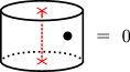
Figure 7. Boerner’s relation

The category $\mathscr{BN}(\mathbb{A})$ is monoidal, with monoidal product given by taking two copies $\mathbb{A}_{1},\mathbb{A}_{2}$ of $\mathbb{A}$ and gluing the boundary component $S^{1}\times\{1\}$ of $\mathbb{A}_{1}$ to the boundary component $S^{1}\times\{0\}$ of $\mathbb{A}_{2}$. The annular TQFT $\mathcal{G}$ is evidently monoidal.

4. Equivariant annular Khovanov homology

We are interested in an annular version of the theory outlined in Section 2.3. Precisely, the goal is to fill in the dashed arrow in the diagram

where the vertical arrows are obtained by setting $\alpha_{0}=\alpha_{1}=0$. Section 4.1 justifies working with the extension $(R_{\alpha},A_{\alpha})$ rather than $(R,A)$. The desired functor $\mathcal{G}_{\alpha}$ is defined in Section 4.2. Maps assigned to saddle cobordisms can be found in (20)–(23). In Section 4.3 we invert $\mathcal{D}$ in the annular theory and show that the rank of the resulting homology depends only on the number of components.

4.1. A preliminary observation

Before defining our equivariant annular TQFT, we note that the $U(2)$-equivariant Frobenius pair $(R,A)$ from Section 2.2 does not admit such a lift, under the minor assumption that modules assigned to circles are free.

The ring $R=\mathbb{Z}[E_{1},E_{2}]$ can be made bigraded, with bidegrees of $E_{1}$ and $E_{2}$ given by $(2,0)$ and $(4,0$), respectively. Let $M$ be a free $\mathbb{Z}\times\mathbb{Z}$-graded $R$-module with basis $m_{-},m_{+}$ in bidegrees $(-1,-1)$ and $(1,1)$, respectively. Suppose $g\colon M\to M$ is an $R$-linear map of bidegree $(2,0)$. Then necessarily

(17) $$g(m_{-})=nE_{1}m_{-}$$

for some $n\in\mathbb{Z}$. In particular, if $M$ is the module assigned to a single essential circle and $g$ is the map assigned to the cobordism in Figure 8, then the relation $X^{2}-E_{1}X+E_{2}=0$ in $A$ implies

(18) $$g^{2}(m_{-})-E_{1}g(m_{-})+E_{2}m_{-}=0.$$

However, (17) and (18) are incompatible.

Figure 8. Dotted product cobordism on an essential circle

4.2. The equivariant annular TQFT $\mathcal{G}_{\alpha}$

Let $\mathscr{BN}_{\alpha}(\mathbb{A})$ denote the Bar-Natan category of the annulus subject to the relations determined by $A_{\alpha}$. Its objects are formal direct sums of formally bigraded collections of simple closed curves in $\mathbb{A}$. Morphisms are matrices whose entries are formal $R_{\alpha}$-linear combinations of dotted cobordisms properly embedded in $\mathbb{A}\times I$, modulo isotopy relative to the boundary, and subject to the local relations shown in Figure 3. The bidegree of a cobordism $S\subset\mathbb{A}\times I$ is given by (10). For an oriented annular link $L$ with diagram $D$, the formal complex $[[D]]$ over $\mathscr{BN}_{\alpha}(\mathbb{A})$ is an invariant of $L$ up to chain homotopy equivalence.

Let $\mathscr{C}\subset\mathbb{A}$ be a collection of circles, and view $\mathscr{C}$ as embedded in $\mathbb{R}^{2}$. Consider $\mathcal{F}_{\alpha}(\mathscr{C})$ with the following additional annular grading, denoted $\operatorname{adeg}$ as in Section 2.3. Define elements of $A_{\alpha}$,

$$v_{0}=1,\hskip 20.00003ptv_{1}=X-\alpha_{0},$$

$$v_{0}^{\prime}=1,\hskip 20.00003ptv_{1}^{\prime}=X-\alpha_{1},$$

with the annular gradings

(19) $$\operatorname{adeg}(v_{0})=\operatorname{adeg}(v_{0}^{\prime})=-1,\hskip 20.00003pt\operatorname{adeg}(v_{1})=\operatorname{adeg}(v_{1}^{\prime})=1.$$

Remark 4.1.

The notation $v_{0},v_{1}$ was also used in Section 3. Setting $\alpha_{0}=\alpha_{1}=0$ in the above expressions recovers $v_{0},v_{1}$ in the non-equivariant setting.

Both $\{v_{0},v_{1}\}=\{1,X-\alpha_{0}\}$ and $\{v_{0}^{\prime},v_{1}^{\prime}\}=\{1,X-\alpha_{1}\}$ is an $R_{\alpha}$-basis for $A_{\alpha}$. Together with the quantum grading, these equip $A_{\alpha}$ with two (isomorphic) structures of a bigraded $R_{\alpha}$-module, with the bigrading given by $(\operatorname{qdeg},\operatorname{adeg})$. The ground ring $R_{\alpha}$ lies in annular degree $0$.

Figure 9. Bigradings, where $\{1,X\}$ corresponds to trivial circles, and $\{v_{0},v_{1}\}$, $\{v_{0}^{\prime},v_{1}^{\prime}\}$ correspond to essential ones. See also Remark 2.4.

Let $\mathscr{C}\subset\mathbb{A}$ consist of $n$ trivial and $m$ essential circles, with the essential circles ordered from innermost (closest to the puncture $\times$) to outermost. Define the annular grading on

$$\mathcal{F}_{\alpha}(\mathscr{C})=A_{\alpha}^{\otimes n}\otimes A_{\alpha}^{\otimes m}$$

by declaring that every copy of $A_{\alpha}$ corresponding to a trivial circle is concentrated in annular degree $0$ and that the copy of $A_{\alpha}$ corresponding to the $i$-th essential circle $(1\leq i\leq m)$ is given the homogeneous basis

$$\{v_{0},v_{1}\}=\{1,X-\alpha_{0}\}$$

if $i$ is odd and

$$\{v_{0}^{\prime},v_{1}^{\prime}\}=\{1,X-\alpha_{1}\}$$

if $i$ is even. In other words, the essential circles are assigned the homogeneous bases $\{1,X-\alpha_{0}\}$ or $\{1,X-\alpha_{1}\}$ in an alternating manner, with the innermost circle assigned $\{1,X-\alpha_{0}\}$. Bigradings are summarized in Figure 9

As in Section 3, it is convenient to distinguish the modules assigned to essential and trivial circles. Let $V_{\alpha}$ and $V^{\prime}_{\alpha}$ denote the module $A_{\alpha}$ with homogeneous bases $\{v_{0},v_{1}\}$ and $\{v_{0}^{\prime},v_{1}^{\prime}\}$, respectively. Then for a collection of circles $\mathscr{C}\subset\mathbb{A}$, the $i$-th essential circle in $\mathscr{C}$ is assigned $V_{\alpha}$ if $i$ is odd and $V_{\alpha}^{\prime}$ if $i$ is even. We reserve the notation $A_{\alpha}$ for the module assigned to a trivial circle. Note that interchanging $\alpha_{0}\leftrightarrow\alpha_{1}$ also interchanges $v_{0}\leftrightarrow v_{0}^{\prime}$ and $v_{1}\leftrightarrow v_{1}^{\prime}$.

Lemma 4.2.

Let $S\subset\mathbb{A}\times I$ be an elementary cobordism. Viewing $S$ as a cobordism in $\mathbb{R}^{2}\times I$, the map $\mathcal{F}_{\alpha}(S)$ splits as a sum

$$\mathcal{F}_{\alpha}(S)=\mathcal{F}_{\alpha}(S)_{0}+\mathcal{F}_{\alpha}(S)_{2}$$

where $\mathcal{F}_{\alpha}(S)_{0}$ preserves $\operatorname{adeg}$ and $\mathcal{F}_{\alpha}(S)_{2}$ increases $\operatorname{adeg}$ by $2$.

Proof.

If the saddle component of $S$ involves only trivial circles then the claim is immediate, since $\mathcal{F}_{\alpha}(S)=\mathcal{F}_{\alpha}(S)_{0}$ in this case. We verify the claim for the four elementary cobordisms in Figure 6 by rewriting $\mathcal{F}_{\alpha}(S)$ in terms of the bases for the circles involved. Terms where $\operatorname{adeg}$ is increased by $2$ are boxed.

$$\begin{split}V_{\alpha}\otimes A_{\alpha}&\xrightarrow{\hyperref@@ii[fig:type1]{\operatorname{(I)}}}V_{\alpha}\\ v_{0}\otimes 1&\mapsto v_{0}\\ v_{1}\otimes 1&\mapsto v_{1}\\ v_{0}\otimes X&\mapsto\alpha_{0}v_{0}+\framebox{$v_{1}$}\\ v_{1}\otimes X&\mapsto\alpha_{1}v_{1}\end{split}$$

$$\begin{split}V_{\alpha}\otimes V_{\alpha}^{\prime}&\xrightarrow{\hyperref@@ii[fig:type2]{\operatorname{(II)}}}A_{\alpha}\\ v_{0}\otimes v_{0}^{\prime}&\mapsto\framebox{$1$}\\ v_{1}\otimes v_{0}^{\prime}&\mapsto X-\alpha_{0}\\ v_{0}\otimes v_{1}^{\prime}&\mapsto X-\alpha_{1}\\ v_{1}\otimes v_{1}^{\prime}&\mapsto 0\end{split}$$

$$\begin{split}V_{\alpha}&\xrightarrow{\hyperref@@ii[fig:type3]{\operatorname{(III)}}}V_{\alpha}\otimes A_{\alpha}\\ v_{0}&\mapsto v_{0}\otimes X-\alpha_{1}v_{0}\otimes 1+\framebox{$v_{1}\otimes 1$}\\ v_{1}&\mapsto v_{1}\otimes X-\alpha_{0}v_{1}\otimes 1\end{split}$$

$$\begin{split}A_{\alpha}&\xrightarrow{\hyperref@@ii[fig:type4]{\operatorname{(IV)}}}V_{\alpha}\otimes V_{\alpha}^{\prime}\\ 1&\mapsto v_{0}\otimes v_{1}^{\prime}+v_{1}\otimes v_{0}^{\prime}\\ X&\mapsto\alpha_{0}v_{0}\otimes v_{1}^{\prime}+\alpha_{1}v_{1}\otimes v_{0}^{\prime}+\framebox{$v_{1}\otimes v_{1}^{\prime}$}\end{split}$$

Our assignment for essential circles depends on nesting, so strictly speaking the above calculations do not handle all cases. However, note that for types (I) and (II), the position of the essential circle does not change, and for types (III) and (IV), the two essential circles involved in the saddle must be consecutive in the ordering. Thus a full verification amounts to interchanging $v_{0}\leftrightarrow v_{0}^{\prime}$, $v_{1}\leftrightarrow v_{1}^{\prime}$ in the input of above maps. One may check that this amounts to interchanging $v_{0}\leftrightarrow v_{0}^{\prime}$, $v_{1}\leftrightarrow v_{1}^{\prime}$, and $\alpha_{0}\leftrightarrow\alpha_{1}$ in the output. ∎

Corollary 4.3.

1. Let $S\subset\mathbb{A}\times I$ be a cobordism. Viewing $S$ as a cobordism in $\mathbb{R}^{2}\times I$, the map $\mathcal{F}_{\alpha}(S)$ splits as a sum

   $$\mathcal{F}_{\alpha}(S)=\mathcal{F}_{\alpha}(S)_{0}+\mathcal{F}_{\alpha}(S)_{+}$$

   where $\mathcal{F}_{\alpha}(S)_{0}$ preserves $\operatorname{adeg}$ and $\mathcal{F}_{\alpha}(S)_{+}$ increases $\operatorname{adeg}$.

2. Let $S_{1},S_{2}\subset\mathbb{A}\times I$ be composable cobordisms. Then

   $$\mathcal{F}_{\alpha}(S_{2}S_{1})_{0}=\mathcal{F}_{\alpha}(S_{2})_{0}\mathcal{F}_{\alpha}(S_{1})_{0}.$$

Proof.

For $(1)$, write $S$ as a composition $S=S_{n}\cdots S_{1}$ where each $S_{i}$ is an elementary cobordism. Functoriality of $\mathcal{F}_{\alpha}$ and Lemma 4.2 yield

$$\mathcal{F}_{\alpha}(S) =\mathcal{F}_{\alpha}(S_{n})\cdots\mathcal{F}_{\alpha}(S_{1})$$

$$=\left(\mathcal{F}_{\alpha}(S_{n})_{0}+\mathcal{F}_{\alpha}(S_{n})_{2}\right)\cdots\left(\mathcal{F}_{\alpha}(S_{1})_{0}+\mathcal{F}_{\alpha}(S_{1})_{2}\right)$$

$$=\mathcal{F}_{\alpha}(S_{n})_{0}\cdots\mathcal{F}_{\alpha}(S_{1})_{0}+\text{terms that increase }\operatorname{adeg}.$$

Therefore

$$\mathcal{F}_{\alpha}(S)_{0}=\mathcal{F}_{\alpha}(S_{n})_{0}\cdots\mathcal{F}_{\alpha}(S_{1})_{0}$$

is the desired $\operatorname{adeg}$-preserving part, and the remaining terms constitute $\mathcal{F}_{\alpha}(S)_{+}$. Statement (2) follows from (1) in a similar fashion. ∎

We are now ready for the main theorem.

Theorem 4.4.

There exists a functor $\mathcal{G}_{\alpha}\colon\mathscr{BN}_{\alpha}(\mathbb{A})\to R_{\alpha}{\rm-}\operatorname{ggmod}$ such that the following diagram commutes

where the vertical arrows are obtained by setting $\alpha_{0}=\alpha_{1}=0$.

Proof.

For a collection of circles $\mathscr{C}\subset\mathbb{A}$, set

$$\mathcal{G}_{\alpha}(S):=\mathcal{F}_{\alpha}(\mathscr{C}),$$

with the bigrading $(\operatorname{qdeg},\operatorname{adeg})$ as defined earlier in this section. For a cobordism $S\subset\mathbb{A}\times I$, set

$$\mathcal{G}_{\alpha}(S):=\mathcal{F}_{\alpha}(S)_{0}$$

as in Corollary 4.3 (1). That $\mathcal{G}_{\alpha}$ is well-defined on cobordisms and factors through the relations in $\mathscr{BN}_{\alpha}(\mathbb{A})$ follows from the analogous statements for $\mathcal{F}_{\alpha}$. Corollary 4.3 (2) implies functoriality of $\mathcal{G}_{\alpha}$. Finally, commutativity of the diagram follows from deleting the boxed terms and setting $\alpha_{0}=\alpha_{1}=0$ in the maps appearing in the proof of Lemma 4.2, and comparing the result with the maps (13)–(16). ∎

Maps assigned to the four elementary saddles in Figure 6 are recorded below. The full set of maps – that is, if other essential circles are present – can be obtained by interchanging $\alpha_{0}\leftrightarrow\alpha_{1}$.

(20) $$\begin{split}V_{\alpha}\otimes A_{\alpha}&\xrightarrow{\hyperref@@ii[fig:type1]{\operatorname{(I)}}}V_{\alpha}\\ v_{0}\otimes 1&\mapsto v_{0}\\ v_{1}\otimes 1&\mapsto v_{1}\\ v_{0}\otimes X&\mapsto\alpha_{0}v_{0}\\ v_{1}\otimes X&\mapsto\alpha_{1}v_{1}\end{split}$$

(21) $$\begin{split}V_{\alpha}\otimes V_{\alpha}^{\prime}&\xrightarrow{\hyperref@@ii[fig:type2]{\operatorname{(II)}}}A_{\alpha}\\ v_{0}\otimes v_{0}^{\prime}&\mapsto 0\\ v_{1}\otimes v_{0}^{\prime}&\mapsto X-\alpha_{0}\\ v_{0}\otimes v_{1}^{\prime}&\mapsto X-\alpha_{1}\\ v_{1}\otimes v_{1}^{\prime}&\mapsto 0\end{split}$$

(22) $$\begin{split}V_{\alpha}&\xrightarrow{\hyperref@@ii[fig:type3]{\operatorname{(III)}}}V_{\alpha}\otimes A_{\alpha}\\ v_{0}&\mapsto v_{0}\otimes X-\alpha_{1}v_{0}\otimes 1\\ v_{1}&\mapsto v_{1}\otimes X-\alpha_{0}v_{1}\otimes 1\end{split}$$

(23) $$\begin{split}A_{\alpha}&\xrightarrow{\hyperref@@ii[fig:type4]{\operatorname{(IV)}}}V_{\alpha}\otimes V_{\alpha}^{\prime}\\ 1&\mapsto v_{0}\otimes v_{1}^{\prime}+v_{1}\otimes v_{0}^{\prime}\\ X&\mapsto\alpha_{0}v_{0}\otimes v_{1}^{\prime}+\alpha_{1}v_{1}\otimes v_{0}^{\prime}\end{split}$$

Let $\mathscr{C}\subset\mathbb{A}$ consist of $m>0$ essential circles, and let $C$ be the $i$-th essential circle in $\mathscr{C}$. Consider the cobordism $S$ whose underlying surface is the identity cobordism $\mathscr{C}\times I$, with a single dot on the component $C\times I$, as shown in Figure 10. Then $\mathcal{G}_{\alpha}(S)$ is the identity on all tensor factors except the one corresponding to $C$, and on $C$ it is given by the left-hand side of (24) if $i$ is odd, and the right-hand side if $i$ is even.

Figure 10. Product cobordism on $m>0$ essential circles, with the $i$-th component dotted

(24) $$\begin{aligned} V_{\alpha}&\to V_{\alpha}\\ v_{0}&\mapsto\alpha_{0}v_{0}\\ v_{1}&\mapsto\alpha_{1}v_{1}\end{aligned} \begin{aligned} V_{\alpha}^{\prime}&\to V_{\alpha}^{\prime}\\ v_{0}^{\prime}&\mapsto\alpha_{1}v_{0}^{\prime}\\ v_{1}^{\prime}&\mapsto\alpha_{0}v_{1}^{\prime}\end{aligned}$$

Observe that the functor $\mathcal{G}_{\alpha}$ is not monoidal, since the action of $X$ on an essential circle depends on its nestedness.

Let $L\subset\mathbb{A}\times I$ be an oriented link with diagram $D$. Let

$$CKh^{\mathbb{A}}_{\alpha}(D):=\mathcal{G}_{\alpha}([[D]])$$

denote the chain complex obtained by applying $\mathcal{G}_{\alpha}$ to the formal complex $[[D]]$. The differential preserves bidegree, and the complex is an invariant of $L$ up to bidegree-preserving chain homotopy equivalence.

The remainder of this section discusses variants of $\mathcal{G}_{\alpha}$. Instead of setting both $\alpha_{0}=\alpha_{1}=0$, it is possible to set only $\alpha_{0}=0$ and rename the remaining parameter $\alpha_{1}$ to $\alpha_{1}=h$. Denote the resulting Frobenius pair by $(R_{h},A_{h})$. Explicitly,

$$R_{h}=\mathbb{Z}[h],\ A_{h}=R_{h}[X]/(X^{2}-hX).$$

It may also be obtained from $(R,A)$ by setting $E_{1}=h$, $E_{2}=0$; note that the obstruction in Section 4.1 disappears when $E_{2}=0$. Collapsing $(R_{h},A_{h})$ further to characteristic $2$ (that is, applying $(-)\otimes_{R_{h}}\mathbb{Z}_{2}[h])$ recovers Bar-Natan’s theory [BN2, Section 9.3]. We expect that the resulting annular homology is related to [TW].

Let $L\subset\mathbb{A}\times I$ be an oriented link with diagram $D$. Viewing $D$ as a diagram in $\mathbb{R}^{2}$ and applying $\mathcal{F}_{\alpha}$ to $[[D]]$ yields a chain complex $CKh_{\alpha}(D)$ of bigraded $R_{\alpha}$-modules. Letting $\partial$ denote the differential, Lemma 4.2 implies that $\partial$ splits as

$$\partial=\partial_{0}+\partial_{2}$$

where $\partial_{0}$ is of bidegree $(0,0)$ and $\partial_{2}$ is of bidegree $(0,2)$. As in [HKLM], we can introduce an extra parameter $\beta$ to account for $\partial_{2}$. Let $R_{\alpha\beta}=R_{\alpha}[\beta]$ with $\beta$ in bidegree $(0,-2)$, and let $CKh_{\alpha\beta}(D)$ be the chain complex over $R_{\alpha\beta}$ with

$$CKh_{\alpha\beta}^{i}(D):=CKh_{\alpha}^{i}(D)\otimes_{R_{\alpha}}R_{\alpha\beta}$$

in homological degree $i$ and differential $\partial_{\beta}$ given by

$$\partial_{\beta}:=\partial_{0}+\beta\partial_{2}.$$

Note that $\partial_{\beta}$ preserves bidegree. Maps assigned to the four elementary saddles in Figure 6 are given below.

$$\begin{split}V_{\alpha}\otimes A_{\alpha}&\xrightarrow{\hyperref@@ii[fig:type1]{\operatorname{(I)}}}V_{\alpha}\\ v_{0}\otimes 1&\mapsto v_{0}\\ v_{1}\otimes 1&\mapsto v_{1}\\ v_{0}\otimes X&\mapsto\alpha_{0}v_{0}+\ \beta v_{1}\\ v_{1}\otimes X&\mapsto\alpha_{1}v_{1}\end{split}$$

$$\begin{split}V_{\alpha}\otimes V_{\alpha}^{\prime}&\xrightarrow{\hyperref@@ii[fig:type2]{\operatorname{(II)}}}A_{\alpha}\\ v_{0}\otimes v_{0}^{\prime}&\mapsto\beta\\ v_{1}\otimes v_{0}^{\prime}&\mapsto X-\alpha_{0}\\ v_{0}\otimes v_{1}^{\prime}&\mapsto X-\alpha_{1}\\ v_{1}\otimes v_{1}^{\prime}&\mapsto 0\end{split}$$

$$\begin{split}V_{\alpha}&\xrightarrow{\hyperref@@ii[fig:type3]{\operatorname{(III)}}}V_{\alpha}\otimes A_{\alpha}\\ v_{0}&\mapsto v_{0}\otimes X-\alpha_{1}v_{0}\otimes 1+\beta v_{1}\otimes 1\\ v_{1}&\mapsto v_{1}\otimes X-\alpha_{0}v_{1}\otimes 1\end{split}$$

$$\begin{split}A_{\alpha}&\xrightarrow{\hyperref@@ii[fig:type4]{\operatorname{(IV)}}}V_{\alpha}\otimes V_{\alpha}^{\prime}\\ 1&\mapsto v_{0}\otimes v_{1}^{\prime}+v_{1}\otimes v_{0}^{\prime}\\ X&\mapsto\alpha_{0}v_{0}\otimes v_{1}^{\prime}+\alpha_{1}v_{1}\otimes v_{0}^{\prime}+\beta v_{1}\otimes v_{1}^{\prime}\end{split}$$

4.3. Inverting $\mathcal{D}$ in equivariant annular homology

Recall the Frobenius pair $(R_{\alpha\mathcal{D}},A_{\alpha\mathcal{D}})$ from [KR], which was reviewed in Section 2.4. Let $\mathcal{G}_{\alpha\mathcal{D}}$ denote the composition

$$\mathscr{BN}_{\alpha}(\mathbb{A})\xrightarrow{\mathcal{G}_{\alpha}}R_{\alpha}{\rm-}\operatorname{ggmod}\to R_{\alpha\mathcal{D}}{\rm-}\operatorname{ggmod}$$

where the second functor is extension of scalars. Consider the following elements of $A_{\alpha\mathcal{D}}$,

$$\overline{v}_{0}:=v_{0}=1,\hskip 20.00003pt\overline{v}_{1}:=\frac{v_{1}}{\alpha_{1}-\alpha_{0}}=\frac{X-\alpha_{0}}{\alpha_{1}-\alpha_{0}},$$

$$\overline{v}_{0}^{\prime}:=v_{0}^{\prime}=1,\hskip 20.00003pt\overline{v}_{1}^{\prime}:=\frac{v_{1}^{\prime}}{\alpha_{0}-\alpha_{1}}=\frac{X-\alpha_{1}}{\alpha_{0}-\alpha_{1}}.$$

Figure 11. Bigradings

As in Section 4.2, let $V_{\alpha\mathcal{D}}$ and $V_{\alpha\mathcal{D}}^{\prime}$ denote the module $A_{\alpha\mathcal{D}}$ with distinguished homogeneous bases $\{\overline{v}_{0},\overline{v}_{1}\}$ and $\{\overline{v}_{0}^{\prime},\overline{v}_{1}^{\prime}\}$, respectively. For a collection of circles $\mathscr{C}\subset\mathbb{A}$, the $i$-th essential circle in $\mathscr{C}$ is assigned $V_{\alpha\mathcal{D}}$ if $i$ is odd and $V_{\alpha\mathcal{D}}^{\prime}$ if $i$ is even. The notation $A_{\alpha\mathcal{D}}$ is reserved for trivial circles, with distinguished basis $\{e_{0},e_{1}\}$, see (8). Bigradings are summarized in Figure 11.

With respect to these bases, the maps assigned to the four elementary saddles in Figure 6 are recorded below.

(25) $$\begin{split}V_{\alpha\mathcal{D}}\otimes A_{\alpha\mathcal{D}}&\xrightarrow{\hyperref@@ii[fig:type1]{\operatorname{(I)}}}V_{\alpha\mathcal{D}}\\ \overline{v}_{0}\otimes e_{0}&\mapsto 0\\ \overline{v}_{1}\otimes e_{0}&\mapsto\overline{v}_{1}\\ \overline{v}_{0}\otimes e_{1}&\mapsto\overline{v}_{0}\\ \overline{v}_{1}\otimes e_{1}&\mapsto 0\end{split}$$

(26) $$\begin{split}V_{\alpha\mathcal{D}}\otimes V_{\alpha\mathcal{D}}^{\prime}&\xrightarrow{\hyperref@@ii[fig:type2]{\operatorname{(II)}}}A_{\alpha\mathcal{D}}\\ \overline{v}_{0}\otimes\overline{v}_{0}^{\prime}&\mapsto 0\\ \overline{v}_{1}\otimes\overline{v}_{0}^{\prime}&\mapsto e_{0}\\ \overline{v}_{0}\otimes\overline{v}_{1}^{\prime}&\mapsto e_{1}\\ \overline{v}_{1}\otimes\overline{v}_{1}^{\prime}&\mapsto 0\end{split}$$

(27) $$\begin{split}V_{\alpha\mathcal{D}}&\xrightarrow{\hyperref@@ii[fig:type3]{\operatorname{(III)}}}V_{\alpha\mathcal{D}}\otimes A_{\alpha\mathcal{D}}\\ \overline{v}_{0}&\mapsto(\alpha_{0}-\alpha_{1})\overline{v}_{0}\otimes e_{1}\\ \overline{v}_{1}&\mapsto(\alpha_{1}-\alpha_{0})\overline{v}_{1}\otimes e_{0}\end{split}$$

(28) $$\begin{split}A_{\alpha\mathcal{D}}&\xrightarrow{\hyperref@@ii[fig:type4]{\operatorname{(IV)}}}V_{\alpha\mathcal{D}}\otimes V_{\alpha\mathcal{D}}^{\prime}\\ e_{0}&\mapsto(\alpha_{1}-\alpha_{0})\overline{v}_{1}\otimes\overline{v}_{0}^{\prime}\\ e_{1}&\mapsto(\alpha_{0}-\alpha_{1})\overline{v}_{0}\otimes\overline{v}_{1}^{\prime}\end{split}$$

To obtain the full set of maps – that is, if other essential circles are present – one interchanges $\alpha_{0}\leftrightarrow\alpha_{1}$, which has the effect of interchanging $\overline{v}_{0}\leftrightarrow\overline{v}_{0}^{\prime}$, $\overline{v}_{1}\leftrightarrow\overline{v}_{1}^{\prime}$, and $e_{0}\leftrightarrow e_{1}$. They are recorded below for convenience.

(29) $$\begin{split}V_{\alpha\mathcal{D}}^{\prime}\otimes A_{\alpha\mathcal{D}}&\to V_{\alpha\mathcal{D}}^{\prime}\\ \overline{v}_{0}^{\prime}\otimes e_{0}&\mapsto\overline{v}_{0}^{\prime}\\ \overline{v}_{1}^{\prime}\otimes e_{0}&\mapsto 0\\ \overline{v}_{0}^{\prime}\otimes e_{1}&\mapsto 0\\ \overline{v}_{1}^{\prime}\otimes e_{1}&\mapsto\overline{v}_{1}^{\prime}\end{split}$$

(30) $$\begin{split}V_{\alpha\mathcal{D}}^{\prime}\otimes V_{\alpha\mathcal{D}}&\to A_{\alpha\mathcal{D}}\\ \overline{v}_{0}^{\prime}\otimes\overline{v}_{0}&\mapsto 0\\ \overline{v}_{1}^{\prime}\otimes\overline{v}_{0}&\mapsto e_{1}\\ \overline{v}_{0}^{\prime}\otimes\overline{v}_{1}&\mapsto e_{0}\\ \overline{v}_{1}^{\prime}\otimes\overline{v}_{1}&\mapsto 0\end{split}$$

(31) $$\begin{split}V_{\alpha\mathcal{D}}^{\prime}&\to V_{\alpha\mathcal{D}}^{\prime}\otimes A_{\alpha\mathcal{D}}\\ \overline{v}_{0}^{\prime}&\mapsto(\alpha_{1}-\alpha_{0})\overline{v}_{0}^{\prime}\otimes e_{0}\\ \overline{v}_{1}^{\prime}&\mapsto(\alpha_{0}-\alpha_{1})\overline{v}_{1}^{\prime}\otimes e_{1}\end{split}$$

(32) $$\begin{split}A_{\alpha\mathcal{D}}&\to V_{\alpha\mathcal{D}}^{\prime}\otimes V_{\alpha\mathcal{D}}\\ e_{0}&\mapsto(\alpha_{1}-\alpha_{0})\overline{v}_{0}^{\prime}\otimes\overline{v}_{1}\\ e_{1}&\mapsto(\alpha_{0}-\alpha_{1})\overline{v}_{1}^{\prime}\otimes\overline{v}_{0}\end{split}$$

These maps may be written uniformly in the following way. Let $\mathscr{C}\subset\mathbb{A}$ be a collection of circles, and label each circle in $\mathscr{C}$ by one of the letters $\mathbf{a}$ or $\mathbf{b}$. From such a labeling we obtain a distinguished basis element of $\mathcal{G}_{\alpha\mathcal{D}}(\mathscr{C})$ by using the correspondence

(33) $$\mathbf{a}\leftrightarrow e_{0},\ \mathbf{b}\leftrightarrow e_{1}$$

for a trivial circle, and

(34) $$\mathbf{a}\leftrightarrow\begin{cases}\overline{v}_{1}&i\text{ is odd}\\ \overline{v}_{0}^{\prime}&i\text{ is even}\end{cases},\ \mathbf{b}\leftrightarrow\begin{cases}\overline{v}_{0}&i\text{ is odd}\\ \overline{v}_{1}^{\prime}&i\text{ is even}\end{cases}$$

on the $i$-th essential circle. Then the saddle maps are

(35) $$\begin{split}V_{\alpha\mathcal{D}}\otimes A_{\alpha\mathcal{D}}&\xrightarrow{\hyperref@@ii[fig:type1]{\operatorname{(I)}}}V_{\alpha\mathcal{D}}\\ \mathbf{b}\otimes\mathbf{a}&\mapsto 0\\ \mathbf{a}\otimes\mathbf{a}&\mapsto\mathbf{a}\\ \mathbf{b}\otimes\mathbf{b}&\mapsto\mathbf{b}\\ \mathbf{a}\otimes\mathbf{b}&\mapsto 0\end{split}$$

(36) $$\begin{split}V_{\alpha\mathcal{D}}\otimes V_{\alpha\mathcal{D}}^{\prime}&\xrightarrow{\hyperref@@ii[fig:type2]{\operatorname{(II)}}}A_{\alpha\mathcal{D}}\\ \mathbf{b}\otimes\mathbf{a}&\mapsto 0\\ \mathbf{a}\otimes\mathbf{a}&\mapsto\mathbf{a}\\ \mathbf{b}\otimes\mathbf{b}&\mapsto\mathbf{b}\\ \mathbf{a}\otimes\mathbf{b}&\mapsto 0\end{split}$$

(37) $$\begin{split}V_{\alpha\mathcal{D}}&\xrightarrow{\hyperref@@ii[fig:type3]{\operatorname{(III)}}}V_{\alpha\mathcal{D}}\otimes A_{\alpha\mathcal{D}}\\ \mathbf{b}&\mapsto(\alpha_{0}-\alpha_{1})\mathbf{b}\otimes\mathbf{b}\\ \mathbf{a}&\mapsto(\alpha_{1}-\alpha_{0})\mathbf{a}\otimes\mathbf{a}\end{split}$$

(38) $$\begin{split}A_{\alpha\mathcal{D}}&\xrightarrow{\hyperref@@ii[fig:type4]{\operatorname{(IV)}}}V_{\alpha\mathcal{D}}\otimes V_{\alpha\mathcal{D}}^{\prime}\\ \mathbf{a}&\mapsto(\alpha_{1}-\alpha_{0})\mathbf{a}\otimes\mathbf{a}\\ \mathbf{b}&\mapsto(\alpha_{0}-\alpha_{1})\mathbf{b}\otimes\mathbf{b}\end{split}$$

Moreover, the same formulas hold with $V_{\alpha\mathcal{D}}$ and $V_{\alpha\mathcal{D}}^{\prime}$ interchanged.

For an annular link $L$ with diagram $D$, let

$$CKh^{\mathbb{A}}_{{\alpha\mathcal{D}}}(D):=\mathcal{G}_{\alpha\mathcal{D}}([[D]])$$

denote the chain complex obtained by applying $\mathcal{G}_{\alpha\mathcal{D}}$ to $[[D]]$. It is an invariant of $L$ up to chain homotopy equivalence, so we may write $Kh^{\mathbb{A}}_{{\alpha\mathcal{D}}}(L)$ to denote the homology of $CKh^{\mathbb{A}}_{{\alpha\mathcal{D}}}(D)$, for any diagram $D$ of $L$.

Theorem 4.5.

Let $L\subset\mathbb{A}\times I$ be a link with diagram $D$. Viewing $L$ as a link in $\mathbb{R}^{3}$, there is a $\operatorname{qdeg}$-preserving isomorphism

$$\varphi\colon CKh^{\mathbb{A}}_{{\alpha\mathcal{D}}}(D)\xrightarrow{\sim}CKh_{{\alpha\mathcal{D}}}(D).$$

Proof.

For a smoothing $D_{u}$, the inclusion $\mathbb{A}\hookrightarrow\mathbb{R}^{2}$ induces an isomorphism

$$\varphi_{u}\colon\mathcal{G}_{\alpha\mathcal{D}}(D_{u})\to\mathcal{F}_{\alpha\mathcal{D}}(D_{u}),$$

defined in terms of the basis elements labeled by $\mathbf{a}$ and $\mathbf{b}$ by

$$\mathbf{a}\mapsto e_{0},\ \mathbf{b}\mapsto e_{1}.$$

Comparing the formulas (35)–(38) with multiplication and comultiplication in $A_{\alpha\mathcal{D}}$, we see that each of the maps $\varphi_{u}$ commute with cobordism maps and thus assemble into an isomorphism $\varphi\colon CKh^{\mathbb{A}}_{{\alpha\mathcal{D}}}(D)\to CKh_{{\alpha\mathcal{D}}}(D)$. It is evident from Figure 11 that each $\varphi_{u}$ preserves $\operatorname{qdeg}$. Quantum grading shifts in both chain complexes are the same, so the isomorphism $\varphi$ preserves $\operatorname{qdeg}$ as well. ∎

The following is immediate from Proposition 2.5.

Corollary 4.6.

For a link $L\subset\mathbb{A}\times I$ with $k$ components, the homology $Kh^{\mathbb{A}}_{{\alpha\mathcal{D}}}(L)$ is a free $R_{\alpha\mathcal{D}}$-module of rank $2^{k}$.

We recall the canonical generators for Lee homology, following [Le] and [Ra]. Let $L\subset\mathbb{A}\times I$ be a link with diagram $D$. Given an orientation $o$ on $L$, let $D_{o}\subset\mathbb{A}$ denote the result of performing the oriented resolution at each crossing,

$$\begin{gathered}\includegraphics{AD_oriented_resolution.pdf}\end{gathered}\,.$$

Each of the resulting circles is naturally oriented. Assign a mod $2$ invariant to each circle $C$ as follows. First, consider the number of circles in $D_{o}$ separating $C$ from infinity, mod $2$. Add $1$ if $C$ is standardly (counterclockwise) oriented, and add $0$ otherwise. Now that each circle in $D_{o}$ is labeled by $0$ or $1$, use the correspondence $0\leftrightarrow\mathbf{a}$, $1\leftrightarrow\mathbf{b}$ to label each circle by $\mathbf{a}$ or $\mathbf{b}$, and finally use (33) and (34) to obtain a generator $\mathfrak{s}_{o}$ in $CKh^{\mathbb{A}}_{{\alpha\mathcal{D}}}(D)$.

For a collection of oriented circles $\mathscr{C}\subset\mathbb{A}$, let $w(\mathscr{C})$ denote the winding number of $\mathscr{C}$. That is, $w(\mathscr{C})$ equals the number of counterclockwise essential circles minus the number of clockwise ones. If $C_{1},\ldots,C_{m}$ are the essential circles in $\mathscr{C}$, then

$$w(\mathscr{C})=\sum_{i=1}^{m}w(C_{i}).$$

Proposition 4.7.

Let $L\subset\mathbb{A}\times I$ be a link with diagram $D$, and let $o$ be an orientation of $L$. Let $m$ be the number of essential circles in the oriented resolution $D_{o}$. Then

$$\operatorname{adeg}(\mathfrak{s}_{o})=(-1)^{m}w(L,o)$$

where $w(L,o)$ is the winding number of $L$ with respect to the orientation $o$.

Proof.

First note that $w(L,o)=w(D_{o})$. It is straightforward to verify that each essential circle $C$ in $D_{o}$ contributes $(-1)^{m}w(C)$ to the annular degree of $\mathfrak{s}_{o}$. The claim follows, since trivial circles do not contribute to the annular degree or the winding number. ∎

5. Dotted Temperley-Lieb category

This section reviews the Temperley-Lieb category $\mathscr{TL}$ and its relation to annular Khovanov homology, following observations in [BPW]. We then introduce a natural equivariant analogue.

For each $n\geq 0$, fix a collection $\underline{n}\subset(0,1)$ of $n$ points in the interior of the unit interval. A planar $(n,m)$-tangle is a smooth embedding of a compact $1$-manifold $M$ into $I\times I$, such that the boundary of $M$ maps to $I\times\{0\}\cup I\times\{1\}$, with $n$ points in $\partial M$ mapping to $\underline{n}\subset I\times\{0\}$, and the remaining $m$ points in $\partial M$ mapping to $\underline{m}\subset\times\{1\}$. Planar tangles are always considered up to isotopy of $I\times I$ fixing the boundary.

Let $\mathscr{TL}$ denote the $\mathbb{Z}[q,q^{-1}]$-linear category whose objects are nonnegative integers. The morphism space $\mathscr{TL}(n,m)$ is freely generated over $\mathbb{Z}[q,q^{-1}]$ by planar $(n,m)$-tangles, modulo the local relation that an innermost circle can be removed at the cost of multiplying the remaining tangle by $q+q^{-1}$,

(39) $$\begin{gathered}\includegraphics{AD_rel_TL.pdf}\end{gathered}\,.$$

Composition is defined by vertically stacking planar tangles. Denote the space of morphisms from $n$ to $m$ by

$$\mathscr{TL}(n,m).$$

The Temperley-Lieb algebra $TL_{n}$ can then be identified with the endomorphism space $\mathscr{TL}(n,n)$. Let $\mathscr{TL}_{q=1}$ denote the category obtained by setting $q=1$.

It was observed in [BPW, Section 6.1] that $\mathscr{TL}$ is closely tied to annular Khovanov homology. By spinning planar tangles in the $S^{1}$ direction, one obtains a functor

(40) $$S^{1}\times(-)\colon\mathscr{TL}_{q=1}\to\mathscr{BN}(\mathbb{A}).$$

Explicitly, $n$ is sent to the essential circles $S^{1}\times\underline{n}\subset\mathbb{A}$, and a planar tangle $T$ is sent to the cobordism $S^{1}\times T$. That $S^{1}\times(-)$ factors through the relation (39) when $q=1$ follows from the fact that a torus in $\mathbb{A}\times I$ evaluates to $2$ in $\mathscr{BN}(\mathbb{A})$. Let

$$\mathscr{BBN}(\mathbb{A})$$

denote the category obtained from $\mathscr{BN}(\mathbb{A})$ by imposing Boerner’s relation, Figure 7. Recall that the non-equivariant annular TQFT $\mathcal{G}$ factors through this relation, so no information is lost from the point of view of link homology.

It is shown in [GLW, Section 4.2] that $\mathcal{G}$ can be made to take values in the representation category of $\mathfrak{sl}_{2}$. On the other hand, it is well-known that Temperley-Lieb diagrams (planar tangles modulo relation (39)) can be interpreted as $U_{q}(\mathfrak{sl}_{2})$-linear maps between tensor powers of the fundamental representation of $U_{q}(\mathfrak{sl}_{2})$; a convenient reference is [BPW, Appendix A.1]. Thus for $q=1$, both $\mathscr{TL}_{q=1}$ and $\mathscr{BBN}(\mathbb{A})$ admit functors $\mathcal{F}_{\mathscr{TL}}$ and $\mathcal{G}$ to $U(\mathfrak{sl}_{2}){\rm-}\operatorname{mod}$. It was observed in [BPW, (6.1)] that the following diagram commutes.

(41)

Moreover, if $\mathscr{TL}_{q=1}$ is made additive and graded by introducing formal direct sums [BN2, Definition 3.2] and formal grading shifts [BN2, Section 6], then the horizontal functor in (41) becomes an equivalence of categories, [BPW, Proposition 6.1].

Thus $\mathscr{TL}_{q=1}$ characterizes the skein category $\mathscr{BBN}(\mathbb{A})$ and the functor $\mathcal{F}_{\mathscr{TL}}$ characterizes the annular TQFT $\mathcal{G}$. On the other hand, $\mathscr{BN}(\mathbb{A})$ was similarly described using planar diagrams in [Ru], which we restate now. A dotted planar $(n,m)$-tangle is a planar $(n,m)$ tangle whose components may be decorated by some number of dots, which are allowed to float freely along a component. Let

$$\mathscr{TL}_{\bullet}$$

denote the category whose objects are nonnegative integers and whose morphisms are $\mathbb{Z}$-linear combinations of dotted planar tangles, modulo the additional local relations in Figure 12.

(a) Undotted circle

(b) Dotted circle

(c) Two dots relation

Figure 12. Relations in $\mathscr{TL}_{\bullet}$.

For a dotted planar tangle $T$, let $T^{u}$ denote the tangle obtained by removing all dots ($u$ stands for undotted). Consider the functor

(42) $$S^{1}\times(-)\colon\mathscr{TL}_{\bullet}\to\mathscr{BN}(\mathbb{A})$$

which sends a dotted planar tangle $T$ to the cobordism whose underlying surface is $S^{1}\times T^{u}$, and which carries $k$ dots on a component if $T$ carried $k$ dots on the corresponding component. The relations in Figure 12 are planar analogues of relations in $\mathscr{BN}(\mathbb{A})$, Figure 1. Figures 12(a) and 12(b) correspond to an undotted torus and a once-dotted torus evaluating to $2$ and $0$ in $\mathscr{BN}(\mathbb{A})$, respectively. Figure 12(c) corresponds to the two dots relation in Figure 1(d).

Upon introducing formal direct sums and formal grading shifts, the argument in [BPW, Proposition 6.1] shows that the functor (42) is essentially surjective and full. It is not faithful, but by [Ru, Theorem 3.1], its kernel is generated by the local relations shown in Figure 13. Note that the second follows from the first by adding a dot near one of the endpoints of the strands and simplifying using the two dots relation.

Figure 13. Russel relations.

To see that the relations hold, consider two annuli embedded in $\mathbb{A}\times I$ with a tube joining them, Figure 14(a), and perform neck-cutting along the two disks shown in Figure 14(b) and Figure 14(c). Denote by

$$\widetilde{\mathscr{TL}}_{\bullet}$$

the category obtained by imposing the Russel relations. It follows from [Ru, Theorem 3.1] that the induced functor

$$S^{1}\times(-)\colon\widetilde{\mathscr{TL}}_{\bullet}\to\mathscr{BN}(\mathbb{A})$$

becomes an equivalence of categories after introducing formal direct sums and formal grading shifts to $\widetilde{\mathscr{TL}}_{\bullet}$.

(a)

(b)

(c)

Figure 14. Two compression disks.

An equivariant version of $\mathscr{TL}_{\bullet}$ follows from considering the skein category $\mathscr{BN}_{\alpha}(\mathbb{A})$. Arguing as in [BPW, Proposition 6.1], any object of $\mathscr{BN}_{\alpha}(\mathbb{A})$ is isomorphic to a direct sum of grading-shifted essential circles. Any cobordism in $\mathscr{BN}_{\alpha}(\mathbb{A})$ can be expressed, in a non-unique way, as an $R_{\alpha}$-linear combination of cobordisms of the form $S^{1}\times T$, where $T$ is a dotted planar tangle. It follows that any additive functor out of $\mathscr{BN}_{\alpha}(\mathbb{A})$ is determined by its value on each collection of $n\geq 0$ essential circles and on cobordisms of the form $S^{1}\times T$. This naturally leads to the following definition.

Definition 5.1.

Let $\mathscr{TL}_{\alpha}$ denote the category whose objects are nonnegative integers, and whose morphisms are formal $R_{\alpha}$-linear combinations of dotted planar tangles, modulo the local relations shown in Figure 15.

For a dotted planar tangle $T$ with $d(T)$ dots, define its degree to be

$$\deg(T)=2d(T).$$

Note that the relations in Figure 15 are homogeneous.

(a) Undotted circle

(b) Dotted circle

(c) Two dots relation

Figure 15. Relations in $\mathscr{TL}_{\alpha}$.

To motivate the relations, consider the functor

(43) $$S^{1}\times(-)\colon\mathscr{TL}_{\alpha}\to\mathscr{BN}_{\alpha}(\mathbb{A})$$

defined as in (42). An undotted torus and a once-dotted torus in $\mathbb{A}\times I$ evaluate to $2$ and $\alpha_{0}+\alpha_{1}$ in $\mathscr{BN}_{\alpha}(\mathbb{A})$, respectively, which explains the relations in Figure 15(a) and Figure 15(b). The relation in Figure 15(c) is a planar analogue of the two dots relation in $\mathscr{BN}_{\alpha}(\mathbb{A})$, see Figure 3(d). A straightforward induction argument also shows that an innermost circle with $k\geq 0$ dots evaluates to $\alpha_{0}^{k}+\alpha_{1}^{k}$ in $\mathscr{TL}_{\alpha}$,

(44) $$\begin{gathered}\includegraphics{AD_TLa_circle_rel.pdf}\,.\end{gathered}$$

By composing (43) with the equivariant annular TQFT $\mathcal{G}_{\alpha}$,

(45) $$\mathscr{TL}_{\alpha}\xrightarrow{S^{1}\times(-)}\mathscr{BN}_{\alpha}(\mathbb{A})\xrightarrow{\mathcal{G}_{\alpha}}R_{\alpha}{\rm-}\operatorname{ggmod},$$

one can view dotted planar tangles as $R_{\alpha}$-linear maps between tensor powers of $A_{\alpha}$.

Remark 5.1.

As is the case for $\mathscr{BN}_{\alpha}(\mathbb{A})$, the relations in $\mathscr{TL}_{\alpha}$ involve only symmetric polynomials in $\alpha_{0}$ and $\alpha_{1}$, so one may consider the $U(2)$-equivariant analogue instead; see also Remark 2.3. However, the functor (45) is not present in the $U(2)$-equivariant setting.

The functor (43) is of course not faithful. For example, it factors through the local relations shown in Figure 16, which are equivariant analogues of the Russel relations, Figure 13. Let

$$\widetilde{\mathscr{TL}}_{\alpha}$$

denote the category obtained from $\mathscr{TL}_{\alpha}$ by imposing the relations in Figure 16 (it suffices to impose only the first).

Figure 16. Equivariant Russel relations.

We end the section with two questions. The first is motivated by [Ru, Theorem 3.1].

Question 1.

Is the induced spinning functor $S^{1}\times(-)\colon\widetilde{\mathscr{TL}}_{\alpha}\to\mathscr{BN}_{\alpha}(\mathbb{A})$ faithful?

By [Ru, Main Theorem] and results in [Kh2], the abelian group $\widetilde{\mathscr{TL}}_{\bullet}(2n,0)$ is free of rank

$$\binom{2n}{n}.$$

Note that for a symbol $\star\in\{\varnothing,\bullet,\alpha\}$, the modules $\mathscr{TL}_{\star}(n,m)$ and $\mathscr{TL}_{\star}(k,\ell)$ are isomorphic whenever $n+m=k+\ell$. An isomorphism $\mathscr{TL}_{\star}(n,m)\to\mathscr{TL}_{\star}(n+m,0)$ and its inverse are depicted in Figure 17. It clearly factors through the Russel relations, so $\widetilde{\mathscr{TL}}_{\bullet}(n,m)$ is free of rank

(46) $$\binom{n+m}{(n+m)/2}$$

whenever $n$ and $m$ have the same parity, and otherwise it is the zero module.

Question 2.

Is $\widetilde{\mathscr{TL}}_{\alpha}(n,m)$ free over $R_{\alpha}$, and, if so, of what rank?

(a) $\mathscr{TL}_{\star}(n,m)\to\mathscr{TL}_{\star}(n+m,0)$

(b) $\mathscr{TL}_{\star}(n+m,0)\to\mathscr{TL}_{\star}(n,m)$

Figure 17. An isomorphism $\mathscr{TL}_{\star}(n,m)\cong\mathscr{TL}_{\star}(n+m,0)$.

Note that $\mathscr{TL}_{\alpha}(n,m)=0$ if $n$ and $m$ have different parities, and otherwise $\mathscr{TL}_{\alpha}(n,m)$ is free of rank

$$2^{\ell}C(\ell),$$

where $\ell=\frac{n+m}{2}$ and $C(\ell)$ is the $\ell$-th Catalan number. To see this, consider the collection of dotted planar $(n,m)$-tangles in which every component carries at most one dot and which has no closed components. They evidently form a basis for $\mathscr{TL}_{\alpha}(n,m)$. There are $C(\ell)$ undotted planar $(n,m)$-tangles with no closed components. A fixed such tangle has $\ell$ components, hence $2^{\ell}$ ways to put at most one dot on each component, which yields the count.

We can find bases for small values. A basis for $\widetilde{\mathscr{TL}}_{\alpha}(1,1)$ is given by an undotted and once-dotted vertical strand, and a basis for $\widetilde{\mathscr{TL}}_{\alpha}(2,2)$ is depicted in (47). That these elements generate the module follows from Figure 16, and linear independence can be verified using $S^{1}\times(-)$ and the TQFT $\mathcal{G}_{\alpha}$. The ranks agree with (46), but it is not clear if this is a coincidence for small examples. For $\widetilde{\mathscr{TL}}_{\alpha}(3,3)$, there are $2^{3}C(3)=40$ generators and many relations, making direct computation difficult.

(47) $$\begin{gathered}\includegraphics{AD_TLa2_basis.pdf}\end{gathered}$$

References

- [APS] M. Asaeda, J. H. Przytycki, and A. Sikora. Categorification of the Kauffman bracket skein module of -bundles over surfaces, Algebr. Geom.Topol. 4:1177–1210, 2004. https://arxiv.org/abs/math/0409414
- [BN1] D. Bar-Natan, On Khovanov’s Categorification of the Jones Polynomial, Algebr. Geom. Topol. 2 (2002), 337-370. https://arxiv.org/abs/math/0201043
- [BN2] D. Bar-Natan, Khovanov Homology for Tangles and Cobordisms, Geom. Topol. 9:1443–1499, 2005. https://arxiv.org/abs/math/0410495
- [BN3] D. Bar-Natan, Fast Khovanov homology computations, J. Knot Th. Ram. 16:243–256, 2007. https://arxiv.org/abs/math/0606318
- [Bo] J. Boerner, A homology theory for framed links in I-bundles using embedded surfaces, Topology Appl. 156, no. 2, 375–391, 2008.
- [BPW] A. Beliakova, K. K. Putyra, and S. M. Wehrli, Quantum Annular Link Homology via Trace Functor I, Invent. Math. 215, 383-492, 2019. https://arxiv.org/abs/1605.03523
- [GLW] J. E. Grigsby, A. Licata, and S. M. Wehrli, Annular Khovanov homology and knotted Schur-Weyl representations, Compos, Math., 154(3), 459-502, 2018. https://arxiv.org/abs/1505.04386
- [HKLM] H. Hunt, H. Keese, A. Licata, and S. Morrison, Computing annular Khovanov homology. https://arxiv.org/abs/1505.04484
- [Kh1] M. Khovanov, A categorification of the Jones polynomial, Duke Math. J.101(3):359–426, 2000. https://arxiv.org/abs/math/9908171
- [Kh2] M. Khovanov, Crossingless matchings and the cohomology of Springer varieties, Communications in Contemporary Math.6 no.2:561–577, 2004. https://arxiv.org/abs/math/0202110
- [Kh3] M. Khovanov, Link homology and Frobenius extensions, Fund. Math., 190:179–190, 2006. https://arxiv.org/abs/math/0411447
- [KR] M. Khovanov and L.-H. Robert, Link homology and Frobenius extensions II. https://arxiv.org/abs/2005.08048
- [Kr] D. Krasner, Equivariant sl(n)-link homology, Algebr. Geom. Topol. 10 no. 1:1 - 32, 2010. https://arxiv.org/abs/0804.3751
- [Le] E. S. Lee, An endomorphism of the Khovanov invariants, Adv. Math.197(2):554-586, 2005. https://arxiv.org/abs/math/0210213
- [MV] M. Mackaay and P. Vaz, The universal -link homology, Algebr. Geom. Topol. 7:1135–1169, 2007. https://arxiv.org/abs/math/0603307
- [Ra] J. Rasmussen, Khovanov homology and the slice genus, Invent. Math., 182(2):419–447, 2010. https://arxiv.org/abs/math/0402131
- [Ro] L. P. Roberts, On knot Floer homology in double branched covers, Geom. Top., 17:413–467, 2013. https://arxiv.org/abs/0706.0741
- [Ru] H. M. Russel, The Bar-Natan skein module of the solid torus and the homology of -Springer varieties, Geom. Dedicata 142:71–89, 2009. https://arxiv.org/abs/0805.0286.
- [TW] L. Truong and M. Zhang, Annular link invariants from the Sarkar-Seed-Szabó spectral sequence. https://arxiv.org/abs/1909.05191
- [We] S. M. Wehrli, A spanning tree model for Khovanov homology, J. Knot Th. Ram. 17 (12):1561-1574, 2008. https://arxiv.org/abs/math/0409328