Interest Clustering Coefficient: a New Metric for Directed Networks like Twitter

Abstract.

We study here the clustering of directed social graphs. The clustering coefficient has been introduced to capture the social phenomena that a friend of a friend tends to be my friend. This metric has been widely studied and has shown to be of great interest to describe the characteristics of a social graph. In fact, the clustering coefficient is adapted for a graph in which the links are undirected, such as friendship links (Facebook) or professional links (LinkedIn). For a graph in which links are directed from a source of information to a consumer of information, it is no more adequate. We show that former studies have missed much of the information contained in the directed part of such graphs. We thus introduce a new metric to measure the clustering of a directed social graph with interest links, namely the interest clustering coefficient. We compute it (exactly and using sampling methods) on a very large social graph, a Twitter snapshot with 505 million users and 23 billion links. We additionally provide the values of the formerly introduced directed and undirected metrics, a first on such a large snapshot. We exhibit that the interest clustering coefficient is larger than classic directed clustering coefficients introduced in the literature. This shows the relevancy of the metric to capture the informational aspects of directed graphs.

1. Introduction

Networks appear in a large number of complex systems, whether they are social, biological, economical or technological. Examples include neuronal networks, the Internet, financial transactions, online social networks, … Most “real-world” networks exhibit some properties that are not due to chance and that are really different from random networks or regular lattices. In this paper, we focus on the study of the clustering coefficient of social networks. Nodes in a network tend to form highly connected neighborhoods. This tendency can be measured by the clustering coefficient. It is classically defined for undirected networks as three times the number of triangles divided by the number of open triangles (formed by two incident edges). This clustering coefficient had been computed in many social networks and had been observed as much higher than what randomness would give. Triangles thus are of crucial interest to understand “real world” networks.

However, a large quantity of those networks are in fact directed (e.g. the web, online social networks like Instagram, financial transactions). It is for instance the case of Twitter, one of the largest and most influential social networks with 126 million daily active users (washington-post, ). In Twitter, a person can follow someone she is interested in; the resulting graph, where there is a link $u\rightarrow v$ if the account associated to the node $u$ followed the account associated to the node $v$, is thus directed. In this study, we used as main dataset the snapshot of Twitter (TS in short) extracted by Gabielkov et al. as explained in (gabielkov2014studying, ) and made available by the authors. The TS has around 505 million nodes and 23 billion arcs, making it one of the biggest snapshots of a social network available today.

The classic definition of the clustering coefficient cannot be directly applied on directed graphs. This is why most of the studies computed it on the so-called mutual graph, as defined by Myers & al. in (myers2014information, ), i.e., on the subgraph built with only the bidirectional links. We call mutual clustering coefficient (mcc for short) the clustering coefficient associated with this graph. We computed this coefficient in the TS, using both exact and approximated methods. We find a value for the mcc of 10,7%. This is a high value, of the same order than the ones found in other web social networks.

However, this classical way to operate leaves out 2/3 of the graph! Indeed, the bidirectional edges only represents 35% of the edges of the TS. A way to avoid it is to consider all links as undirected and to compute the clustering coefficient of the obtained undirected graph. We call undirected clustering coefficient (ucc for short) the corresponding computed coefficient. Such a computation in the TS gives a value of ucc of only 0.11%. This is way lower than what was found in most undirected social networks. It is thus a necessity to introduce specific clustering coefficients for the directed graphs. More generally, when analyzing any directed datasets, it is of crucial importance to take into account the information contained in its directed part in the most adequate way.

A first way to do that is to look at the different ways to form triangles with directed edges. Fagiolo computed the expected values of clustering coefficients considering directed triangles for random graphs in (fagiolo2007clustering, ) and illustrated his method on empirical data on world-trade flows. There are two possible orientations of triangles: transitive and cyclic triangles, see Figures 1(b) and 1(c). Each type of triangles corresponds to a directed clustering coefficient :

• the transitive clustering coefficient (tcc in short), defined as:

  $$tcc=\frac{\text{\# transitive triangles}}{\text{\# open transitive triangles}},$$

• the cyclic clustering coefficient (ccc in short), defined as:

  $$ccc=\frac{3\cdot\text{\# cyclic triangles}}{\text{\# open transitive triangles}}.$$

We computed both coefficients for the snapshot, obtaining $tcc=1.9\%$ and $ccc=1.7\%$. However, note that a large part of the transitive and cyclic triangles comes from bidirectional triangles. When removing them, we arrive to values of $tcc=0.51\%$ and $ccc=0.24\%$.

We believe those metrics miss an essential aspect of the Twitter graph: while the clustering coefficient were defined to represent the social cliques between people, it is not adequate to capture the information aspect of Twitter, known to be both a social and information media (kwak2010twitter, ; myers2014information, ). In this work, we go one step further in the way directed relationships are modeled. We argue that in directed networks, the best way to define a relation or similarity between two individuals (Bob and Alice) is not always by a direct link, but by a common interest, that is, two links towards the same node (e.g., Bob $\rightarrow$ Carol and Alice $\rightarrow$ Carol). Indeed, when discussing interests, consider two nodes having similar interests. Apart from being friends, these two nodes do not have any reason to be directly connected. However, they would tend to be connected to the same out-neighbors. We exploit this to study a new notion of connections in directed networks and the new naturally associated clustering coefficient, which we name interest clustering coefficient, or icc in short, and define as follows:

$${\tt icc}=\frac{4\cdot\text{\# K22s}}{\text{\# open K22s}},$$

where a K22 is defined as a set of four nodes in which two of them follow the two others, and an open K22 is a K22 with a missing link, see Figure 1(d). We computed the icc on the Twitter snapshot, obtaining ${\tt icc}=3.6\%$ ($3.1\%$ when removing the bidirectional structures). This value, an order of magnitude higher than the previous clustering coefficients computed on the non bidirectional directed graph, confirm the interest of this metric. If the clustering coefficient of triangles are good metrics to capture the social aspect of a graph, the interest clustering coefficient is a good metric to capture the informational aspect.

In summary, our contributions are the following:

• We define a new clustering coefficient for graphs with interest links.

• We succeeded in computing it, both exactly and using sampling methods, for a snapshot of Twitter with 505 million nodes and 23 billion edges.

• We additionally provide the values of the directed and undirected clustering coefficients previously defined in the literature. We believe this is the first time that such coefficients are computed exactly for a large directed online social network.

• We compute this new metric as much as the previous ones on other directed datasets to highlight the differences and interests of the different metrics.

• We then propose a new random graph model to obtain random directed graphs with a high interest clustering coefficient. We prove this model follows power-law in- and out-degree distributions, and analyse the interest clustering coefficient value by simulation.

• Lastly, we discuss the usage of this new metric for link recommendation. The principle is to recommend links closing a large number of K22s (instead, classically, of triangles). We discuss the strengths/weaknesses of this method for a set of Twitter users.

The paper is organized as follows. We first discuss related work in Section 2. In Section 3, we present the algorithms we used to compute the values of the interest clustering coefficient, both exactly and by sampling. We discuss the results on the clustering coefficients of Twitter in Section 4, and of other directed datasets in Section 5. In section 6, we propose and study a preferential attachment model providing a high interest clustering coefficient. Lastly, we discuss the use of interest clustering coefficient for link recommendation in Section 7.

(a) Undirected triangles.

(b) Transitive directed triangles.

(c) Cyclic directed triangles.

(d) K22s.

Figure 1. Closed (left) and open (right) undirected and directed triangles and K22s.

2. Related Work

Complex networks. Even if the study of complex networks is an old field (strogatz2001exploring, ), it keeps receiving a lot of attention from the research community. The reason for this is twofold. First, a great number of very large practical systems emerged recently can be seen as complex networks, in particular online social media networks, see (lu2011link, ) for a survey. Second, with the development of big data analysis, entrepreneurs, analysts or researchers have new tools to study those huge amounts of data. Complex networks often exhibit common properties, like small diameter (albert2002statistical, ), small average distance (watts1998collective, ; backstrom2012four, ; leskovec2008planetary, ), heavy tail degree distributions (clauset2009power, ; leskovec2008planetary, ), high clustering (watts1998collective, ), communities (ugander2011anatomy, ), etc.

Clustering coefficient. Among those properties, the clustering coefficient shows that, when two people know each other, there is a high probability that those people have common friends. The clustering coefficient has numerous important applications, such as spam detection (boykin2005leveraging, ), link recommendation (silva2010graph, ; chen2009make, ), information spread (granovetter1977strength, ), study of biased network samples (newman2003ego, ), performance of some neural networks (kim2004performance, ) , etc. There are different definitions of the clustering coefficient. The global clustering coefficient, sometimes also called transitivity, was first introduced by Barrat and Weigt in (barrat2000properties, ). It is defined as

$$CC_{g}=3\times\frac{\text{\# triangles in the graph}}{\text{\# connected triplets of vertices in the graph}}.$$

Another definition was given by Watts and Strogatz (watts1998collective, ) and is called the local clustering coefficient. It is defined as the mean over all nodes of the graph of the local clustering of each node, that is the probability that two random neighbors of the node are also connected together. We use the global clustering coefficient in this paper. The clustering coefficient has also been defined for weighted graphs (saramaki2007generalizations, ; opsahl2009clustering, ). The local clustering coefficient of a node i, first introduced by Watts and Strogatz (watts1998collective, ), is defined as the probability that two neighbors of i are also connected together. This probability can be computed as

$$CC(i)=\frac{\text{\# triangles with the node i}}{\text{\# connected triplets centered on i}},$$

where (# connected triplets centered on i) = $\binom{\text{deg(i)}}{2}$. From here can be defined for the whole graph a clustering coefficient as the mean of the local clustering coefficients over all the nodes of the graph:

$$CC_{g1}=\frac{1}{n}\sum\limits_{i\in V}CC(i)$$

Another definition was first introduced by Barrat and Weigt in (barrat2000properties, ), and is called the global clustering coefficient, or transitivity. It is defined as

$$CC_{g}=3\times\frac{\text{\# triangles in the graph}}{\text{\# connected triplets of vertices in the graph}}.$$

We use the global clustering coefficient in this paper. The clustering coefficient has also been defined for weighted graphs (saramaki2007generalizations, ; opsahl2009clustering, ).

Computations for social graphs. The undirected clustering coefficient of some social networks has been provided in the literature. It has been computed on very large snapshots for Facebook (ugander2011anatomy, ), Microsoft Messenger (leskovec2008planetary, ), Flickr, and YouTube (mislove2007measurement, ). The local clustering coefficient has also been studied in the undirected mutual graph of Twitter (myers2014information, ). We can also cite the values given by the Network Repository project (rossi2015network, ), providing a large comprehensive collection of network graph data available for which it lists some basic properties. The undirected clustering coefficient is usually much higher in social networks than in random models.

Directed graphs. All these studies only consider the undirected clustering coefficient, even for directed graphs like Twitter. Fagiolo introduced definitions of directed clustering coefficients, that we named tcc and ccc (fagiolo2007clustering, ), but those definitions had never been computed and discussed on large datasets to our knowledge, as we do in this paper. Moreover, we believe that these metrics are not the most relevant ones for directed graphs with interest links.

Computing substructures. Researchers studied methods to efficiently compute the number of triangles in a graph, as naive methods are computationally very expensive on large graphs. Two families of methods have been proposed: triangle exact counting or enumeration and estimations. In the first family, the fastest algorithm is due to Alon, Yuster, and Zwick (alon1997finding, ) and runs in $O(m^{1.41})$, with m the number of edges. $O(m^{\frac{2\omega}{\omega+1}})$, with m the number of edges and $\omega$ the best known exponent for the fast matrix multiplication. Its current value is 2.3728, due to an algorithm of (coppersmith1987matrix, ) improved by (le2014powers, ), giving a complexity of $O(m^{1.41})$ for the AYZ algorithm. However, methods using matrix multiplication cannot be used for large graphs because of their memory requirements. In practice, enumeration methods are often used, see e.g., (latapy2008main, ; schank2005finding, ). A large number of methods for approximate counting were proposed, see for example (kolountzakis2012efficient, ) and its references. The authors obtain a running time of $O(m+\frac{m^{3/2}\log n}{t\varepsilon^{2}})$ and a $(1\pm\varepsilon)$ approximation. Methods to count rectangles and butterfly structures in undirected bipartite networks were also proposed in (wang2014rectangle, ) and in (sanei2018butterfly, ). In this paper, we propose an efficient enumeration algorithm to count the number of K22s and open K22s in a very large graph. We focused on the case in which only one adjacency can be stored, as this was our case for the TS. To the best of our knowledge, we are the first to consider this setting.

3. Computing Clustering Coefficients in Twitter

We computed the interest clustering coefficient and the triangle clustering coefficients on a directed Twitter snapshot (TS in short) that we use as a typical example of a directed social network with interest links. We used two different methods: an exact count and an estimation using sampling techniques, either with a Monte Carlo algorithm or with a sampling of the graph.

3.1. The Twitter Snapshot

In order to compute the different clustering coefficients of a real graph, the authors of (gabielkov2012complete, ) gave us access to a snapshot of the graph of the followings of Twitter. The snapshot was collected between March 2012 and July 2012. With $n=505$ million nodes and $m=24$ billion links collected, this graph is the largest directed social network graph available today, to the best of our knowledge. Each node of the graph represents an account of Twitter, and there is a link between two nodes $u$ and $v$, if the account $u$ follows the account $v$. All account IDs have been anonymized. The snapshot is a perfect case study as Twitter is a directed social network used both as a social and an information network (myers2014information, ; kwak2010twitter, ). It allows to study directed/undirected social/interest clustering coefficients.
Degree distributions of the Twitter Snapshot.

Figure 2. In- (Top) and out-degree (Bottom) distributions of the Twitter Snapshot. The obtained distribution is given by the blue points; the black crosses represent the logarithmic binning of the distribution (a mean of a given amount of points on a logarithmic scale). The red straight line is the fit of the logarithmic binning; it has slopes of $-2.174$ and $-2.762$ for the in and out degree distribution.

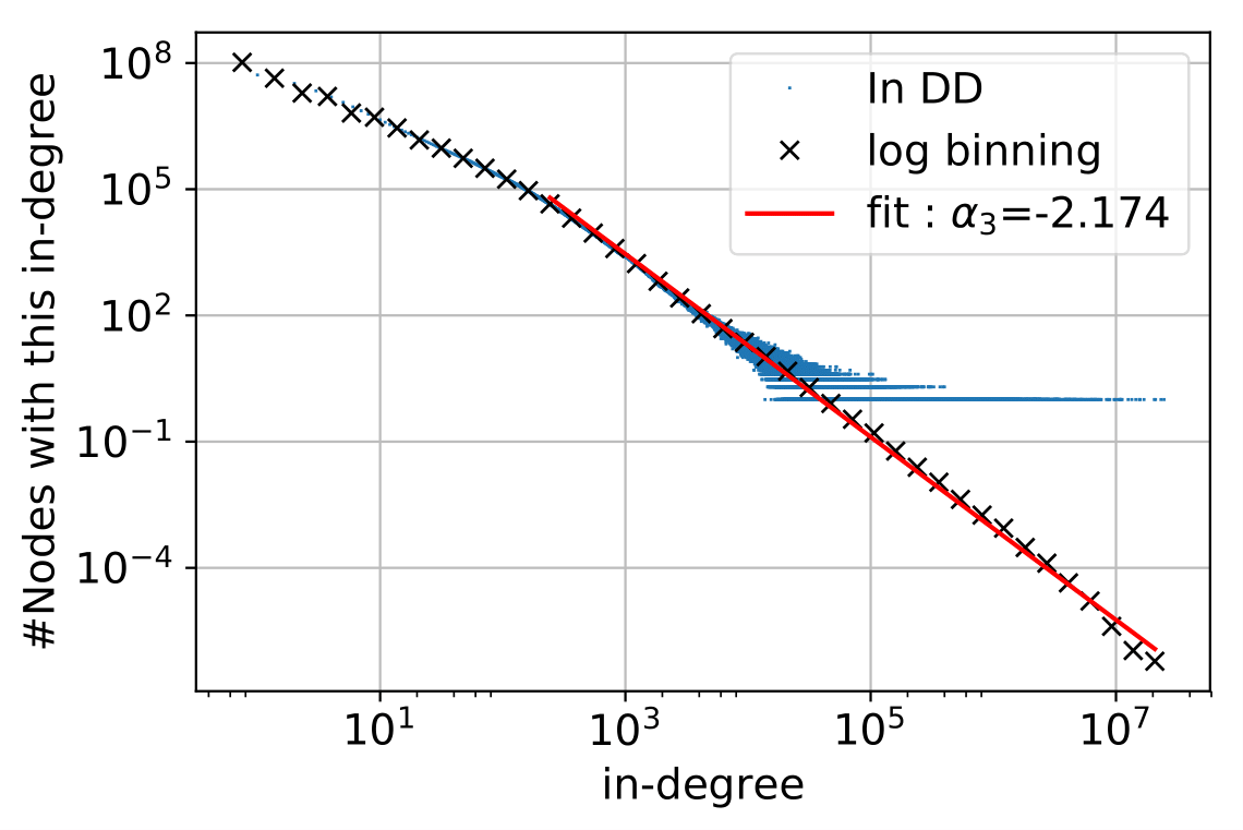
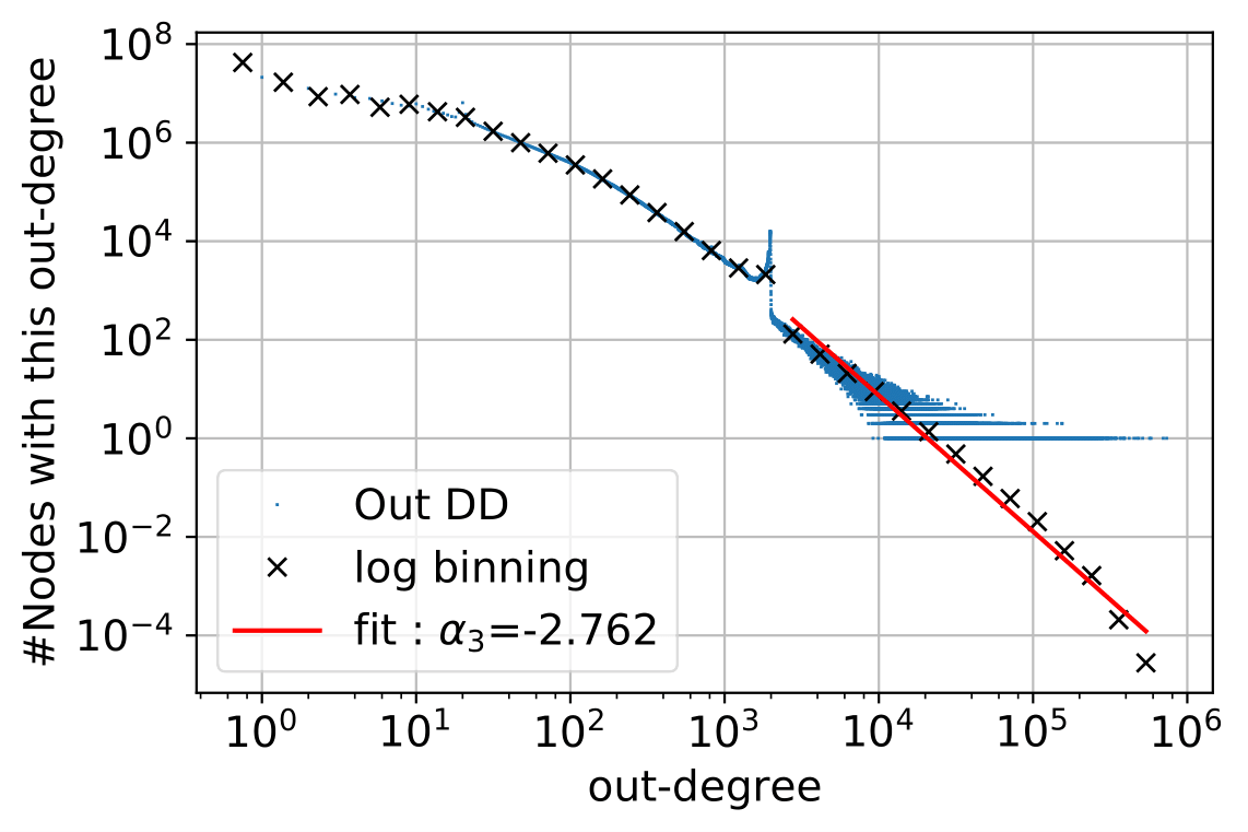
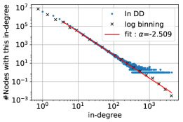
We provide in Figure 2 the degree distributions of the TS. We fitted their tails to power law distributions. We obtained $P^{-}(i)=C^{-}i^{-2.17}$ and $P^{+}(i)=C^{+}i^{-2.76}$, with $P^{-}(i)$ (respectively $P^{+}(i)$) the probability that a node has in-degree (resp. out-degree) $i$. In the following, we use the obtained values to compute the practical complexity of the algorithms.
Other references of the literature have also provided a power law fit for both distributions, see e.g., (myers2014information, ). In this work, the authors obtained exponents of values 1.35 and 1.28. However, we believe that the authors did a fit on the complete distributions and not on their tails, leading to power law exponents below 2. This is why we preferred to only fit the tail. Another point of discussion would be to decide if the out-degree distribution really behaves as a power law. However, the best fit of the distributions is out of the scope of this paper. We just used the values provided by our fit as a possible model of the graph, but others exist.

3.2. Exact Count

We computed the exact numbers of K22s and open K22s in the Twitter Snapshot. Recall that we are discussing a dataset with hundreds of million nodes and billions of arcs. [Fred: should we put it? if yes, we should be coherent everywhere] Since 21.3% of the accounts of the TS have a null in-degree and out-degree (gabielkov2014studying, ), if we remove those vertices, we are left to the study of a network with $n=396$ million nodes and $a=24$ billion arcs. Results are reported in Table 1 and discussed in Section 4. We also retrieved the number of directed and undirected triangles of TS. We first discuss the complexity of algorithms for exact counting on very large graphs. We then present the algorithms we use and discuss the results.

In the rest of this paper, we call top vertices (resp. bottom vertices) of a K22 the vertices which are destinations (resp. sources) of the K22 edges. We call a fork a set of two edges of a K22 connected to the same vertex. We say that a fork has top (or bottom) vertex $x$ if both edges are connected to $x$ and $x$ is a top (resp. bottom) vertex of the K22. The same terminology applies to open K22s.

Trivial algorithm. The trivial algorithm would consider all quadruplets of vertices with 2 upper vertices. Then, for each quadruplet, it would check the existence of a K22 and of open K22s. There are $\binom{4}{2}\binom{n}{4}$ such quadruplets. It thus gives a complexity of $O(n^{4})$. This method can thus not be considered for the TS as it would perform $6.4\text{\times}{10}^{33}$ iterations.

Improved algorithm. The practical complexity can be greatly improved by only considering connected quadruplets, and by mutualizing the computations of the common neighbors of the in-neighbors of a vertex, as explained below. The pseudo-code is given in Algorithm 1.
The algorithm’s main loop iterates on the vertices of the graph. For each vertex $x$, we consider its in-neighborhood $N^{-}(x)$. We then compute how many times a vertex $w$ (with $w<x$ to avoid counting a K22 twice) appears in the out-neighborhoods of the vertices of $N^{-}(x)$. We denote it $\#occ(w)$. We use a hash table to store the value of $\#occ(w)$ in order to be able to do a single pass on each out-neighbor.
For a vertex $w$, any pair of its $\#occ(w)$ in-neighbors common with $x$ forms a K22 with $x$ and $w$ as bottom vertices. There are hence $\binom{k}{2}$ K22s with $x$ and $w$ as bottom vertices. The number of K22s with $x$ as a top vertex is then

$$\#K22(x)=\sum_{w|\#occ(w)\geq 2}\binom{\#occ(w)}{2}.$$

The number of open K22s with $x$ as the top vertex is computed by noticing that, for any pair of vertices $u$ and $v$ of $N^{-}(x)$, we have $d^{+}(u)-1+d^{+}(v)-1-\mathds{1}_{v\in N^{+}(u)}-\mathds{1}_{u\in N^{+}(v)}$ open K22s containing this fork $(ux,vx)$. We can count the number of open K22s with $x$ as a top vertex, $u$ as the bottom vertex of out-degree 2 (and thus another vertex $v$ as the bottom vertex of out-degree 1). A vertex $u\in N^{-}(x)$ is thus in $(d^{+}(u)-1\sum_{v\in N^{-}(x)\setminus\{u\}}1_{v\in N^{+}(u)})(d^{-}(x)-1)$ such open K22s. The only subtlety is that we count the number of arcs, which are between two vertices of $N^{-}(x)$, during the loop on the out-neighborhoods of the vertices of $N^{-}(x)$. We note this number #internalArcs. We then have:

$$\#openK22(x)=\left(\sum_{u\in N^{-}(x)}(d^{+}(u)-1)(d^{-}(x)-1)\right)-\#internalArcs.$$

Lastly, the global number of K22s (resp. open K22s) in the digraph is just the sum of the number of K22s (resp. open K22s) with a vertex $x$ as a top vertex, as, since we only consider K22s formed with a vertex $w$ such that $x<w$, we only count each K22 once.

Algorithm 1 Enumeration of K22s and open K22s

1:$\rhd$

2:Input: Digraph$(V,A)$

3:#occ=0 $\triangleright$ hash table

4:for $x\in V$ do

5:     $\#internalArcs\leftarrow 0$ $\triangleright$ We count the number of arcs internal to $N^{-}(x)$ as these arcs do not form open K22s

6:     for $v\in N^{-}(x)$ do

7:         #openK22s $+=(d^{+}(v)-1)(d^{-}(x)-1)$

8:         for $w\in N^{+}(v)\setminus\{x\}$ do

9:              #occ$[w]+=1$

10:              if $w\in N^{-}(x)$ then $\triangleright$ We use a second hash table to test that.

11:                  $\#internalArcs+=1$                             

12:     for $w$ with #occ$[w]\geq 2$ do

13:         #k22$+=\binom{\#occ[w]}{2}$      

14:     #openK22s $-=\#internalArcs$

15:     $\#occ\leftarrow 0$ $\triangleright$ Done with a double loop

16:icc $\leftarrow\frac{4\#K22}{\#openK22}$

[Fred: Should we put them in appendix?]

• As the graph is stored as a table of lists of neighbors, we do not have access in $O(1)$ to the information that $u$ belongs to a neighborhood $N^{-}(x)$. We can get it in $O(\log_{2}(d-(x)))$ by doing a search by dichotomy. We preferred to avoid this, and thus we use two hash tables:

  • A hash table to store the number of occurrences of a vertex $w$ in the out-neighborhoods of the vertices of $N^{-}(x)$.

  • A hash table to store $N^{-}(x)$ to compute the internal arcs.

• We avoid some multiplications by:

  • computing $2\cdot\#K22(x)=\#occ[w]\break\cdot(\#occ[w]-1)$. We then get at the end 2 times the number of K22s. We just have to multiply by 2 and divide by the #openK22s to obtain icc.

  • We avoid $d^{-}(x)$ multiplications of line 7 by doing it only once per vertex on line 14.

• We re-initialize the table #occ by using the same double loop on the out-neighborhoods of the vertices of $N^{-}(x)$ to avoid iterating on the table.

Complexity of the used algorithm. The complexity thus is $m+\sum_{u}d^{+}(u)(d^{+}(u)-1)$. Indeed, each edge is only considered once as an in-arc and $d^{+}-1$ times as an out-arc. Note that, in the Twitter Snapshot, the sum of the squares of the degrees is equal to $8\cdot 10^{13}$. The order of the number of iterations needed to compute the number of K22s was thus massively decreased from the $6.4\text{\times}{10}^{33}$ iterations of the trivial algorithm.

graph following a power-law degree distribution A main characteristic of the real networks is their heavy-tailed degree distribution: most of them have a power-law degree distribution  (clauset2009power, )  (newman2018networks), with a power exponent between 2 and 3. It is known that the maximum degree of a power-law distribution $P(i)=Ci^{-a}$ is in $O(n^{\frac{1}{a-1}})$ (cohen2000resilience). Complexity on graphs following a power-law degree distribution. Complexity on graphs following a power-law degree distribution. The complexity of the algorithm on a graph built with preferential attachment can be computed as follows. We consider without loss of generality that the sum of the square of the degrees is minimum for the out-degrees (and not the in-degrees). The maximum degree is $d^{+}_{\max}=O(n^{1/(\alpha^{+}-1)})$, with $\alpha^{+}$ the exponent of the out-degree power law distribution. Thus, the sum of the squares of the degrees, when $2\leq\alpha^{+}<3$, is $\sum_{v\in V}(d^{+}(v))^{2}$ = $C^{+}n\sum_{i=1}^{d^{+}_{\max}}\frac{i^{2}}{i^{\alpha^{+}}}$ $\underset{n\to\infty}{\sim}$ $C^{+}n\int_{i=1}^{d^{+}_{\max}}\frac{1}{i^{\alpha^{+}-2}}$ = $\left[\frac{C^{+}n}{(3-\alpha^{+})i^{\alpha^{+}-3}}\right]_{1}^{d^{+}_{\max}}$ $\simeq$ $\frac{C^{+}n}{(3-\alpha^{+}){d^{+}_{\max}}^{\alpha^{+}-3}}$ = $\frac{C^{+}}{(3-\alpha^{+})}n^{1+\frac{3-\alpha^{+}}{\alpha^{+}-1}}$, where $C^{+}=\frac{1}{\sum_{i\in\mathbb{N}^{+}}i^{\alpha^{+}}}$. The complexity is thus in $O(m+n^{1+\frac{3-\alpha^{+}}{\alpha^{+}-1}})$. For preferential attachment graphs with exponents between 2 and 3, this gives a complexity between $O(m+n)$ and $O(n^{2})$, to be compared to the one of the naive method $O(n^{4})$. Discuter de l’AN
Note that the number of undirected and directed triangles can be easily computed while counting the K22s. We do not present how here due to lack of space.

Counting the number of triangles. The number of transitive triangles can easily be computed for free while counting the K22s. When iterating over the vertices of the TS and considering the vertex $x$ in Algorithm 1, the number internal_arcs of arcs between vertices of $N^{-}(x)$ corresponds to the number of transitive triangles for which $x$ is the top vertex. The number of open transitive triangles with $x$ as the top vertex is simply $d^{-}(x)\cdot d^{+}(x)$. The total number of open transitive triangles is then just the sum of this quantity over all $x$. The number of cyclic triangles for $x$ can also be easily computed by counting the number of arcs from $N^{+}(x)$ to $N^{-}(x)$. Each cyclic triangle is counted three times. The number of open cyclic triangles is the same as the number of transitive triangles. We can compute the number of undirected triangles with similar methods (either on the full (but undirected) graph or on the mutual graph).

Complexity of the triangle counting could be computed precisely.

Note that the fastest methods to compute triangles in graphs have a complexity of $O(m^{1.41})$, where $m$ is the number of edges  (alon1997finding, ). These methods rely on fast matrix multiplications and cannot be applied for large graphs as they need to have the full matrix in memory. Moreover, our algorithms would be faster in practice for large complex networks as they are sparse graphs. The average indegree (or outdegree) has a low value of 45.6 (gabielkov2014studying, ) in Twitter. The complexity of the matrix methods would be of the order of $3.2\cdot 10^{14}$ for the TS as $m=2.3\cdot 10^{10}$. This is higher than the practical complexity of computing the exact number of K22s (which is itself higher than the complexity of computing triangles). We discuss the obtained results with the exact count in Section 4.

[Fred: be careful $O(constant)$]

3.3. Approximate Counts

As discussed later in Section 4, the exact count of the number of K22s and open K22s in Twitter implies massive computations. This number can be estimated using Monte Carlo Method and/or computations on a sample of the graph. We discuss both methods below. One of our goals was to see how good computations made in the literature using smaller Twitter snapshots were.

3.3.1. Exact icc on Twitter Samples.

Figure 3. Estimation of the K22s (Top), open K22s (Middle) and interest clustering coefficient (Bottom) for different sample sizes.

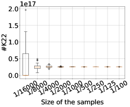
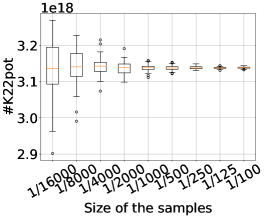
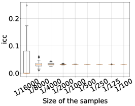
We built samples of the TS to estimate the interest clustering coefficient. Several choices can be made to build the samples. To avoid missing nodes of high degrees (which would lead to a high variance), we sampled the arcs (and not the nodes). Given a sampling probability $p$, we keep an arc in the sample with probability $p$. We generated samples of different sizes corresponding to sampling probabilities from $p=1/100$ to $p=1/16000$.

[Fred: the following is too detailed]

Estimator of the number of K22 and open K22s. Let us call $\mathcal{A}$ the set of occurrences of a specific pattern (in our case, either a K22 or an open K22). The number of occurrences of the pattern in a sample, $X$, is given by $X=\sum_{A\in\mathcal{A}}X_{A}$, where $X_{A}$ is the random variable which is equal to $1$ if all the arcs of pattern $A$ are selected in the sample and $0$ otherwise.
If we note $l$ the number of arcs of the pattern (4 for a K22 and 3 for an open K22), we have that $\mathcal{P}[X_{A}=1]=p^{l}$. By linearity of the expectation, we get $E[X]=p^{l}|\mathcal{A}|.$

$$E[X]=p^{l}|\mathcal{A}|$$

Thus, $Y=p^{-l}X$ is an unbiased estimator of $|\mathcal{A}|$. We succeeded to give theoretical bounds on the variance of this estimator. The difficulty was that the random variables $X_{A}$ are not independent, i.e., two K22s can share a common link. Otherwise, the variance would simply be $\mathbb{V}(X)=\sum_{A\in\mathcal{A}}\mathbb{V}[X_{A}]=|\mathcal{A}|p^{l}(1-p^{l})\leq|\mathcal{A}|p^{l}$. However, we argued that (and we later verified that), in practice, most of the K22s and open K22s do not share any link. The theoretical bounds can be found in annex LABEL:Annex:edge_sample.

Variance. Note that the random variables $X_{A}$ are not independent, i.e., two K22s can share a common link. Otherwise, the variance would simply be $\mathbb{V}(X)=\sum_{A\in\mathcal{A}}\mathbb{V}[X_{A}]=|\mathcal{A}|p^{l}(1-p^{l})\leq|\mathcal{A}|p^{l}$. However, we can argue that (and we will verify that), in practice, most of the K22s and open K22s do not share any link. It can be used in the analysis as follows.

$$\mathbb{V}[X] =E[X^{2}]-E[X]^{2}=E[(\sum_{A\in\mathcal{A}}X_{A})^{2}]-E[X]^{2}$$

$$=\sum_{(A,B)\in\mathcal{A}}E[X_{A}X_{B}]-E[X]^{2}$$

$$\mathbb{V}[X] =E[X^{2}]-E[X]^{2}$$

$$=E[(\sum_{A\in\mathcal{A}}X_{A})^{2}]-E[X]^{2}$$

$$=\sum_{(A,B)\in\mathcal{A}}E[X_{A}X_{B}]-E[X]^{2}$$

We now distinguish the couples of dependent patterns, which we note $\Delta=\{(A,B)\mid A\cap B\neq\emptyset\}$, from the ones of independent ones, ${\bar{\Delta}}=\{(A,B)\mid A\cap B=\emptyset\}$.

$$V[X] =\sum_{(A,B)\in{\bar{\Delta}}}E[X_{A}X_{B}]+\sum_{(A,B)\in\Delta}E[X_{A}X_{B}]-E[X]^{2}$$

When $A$ and $B$ are independent, we have

$$E[X_{A}X_{B}]=\mathbb{E}[X_{A}]\mathbb{E}[X_{B}]=p^{2l}.$$

As $E[X]^{2}=p^{2l}|\mathcal{A}|^{2}$, we get

$$V[X] =\sum_{(A,B)\in{\bar{\Delta}}}E[X_{A}]E[X_{B}]+\sum_{(A,B)\in\Delta}E[X_{A}X_{B}]-E[X]^{2}$$

$$=\sum_{(A,B)\in\Delta}(E[X_{A}X_{B}]-p^{2l})$$

Let us now distinguish different cases. We note $\Delta_{i}$ the set of couples of patterns sharing $1\leq i\leq l$ arcs. For a couple $(A,B)\in\Delta_{i}$, we have that $\mathbb{E}[X_{A}X_{B}]=p^{2l-i}$, giving that

$$\mathbb{V}[X]\leq\sum_{i=1}^{l}\sum_{(A,B)\in\Delta_{i}}(p^{2l-i}-p^{2l}).$$

Since $p<1$, we get

$$\mathbb{V}[X]\leq\sum_{i=1}^{l}p^{2l-i}\left|\Delta_{i}\right|.$$

Note that, when all patterns are independent, $\left|\Delta\right|=|\Delta_{l}|=|\mathcal{A}|$ (couples $(A,A)\in\mathcal{A}$), giving back the variance of the independent case, $p^{l}|\mathcal{A}|$. Chebycheff’s inequality tells us that:

$$Prob[|Y-\mu|\geq k\sigma]\leq\frac{1}{k^{2}},$$

where $\mu$ is the expectation and $\sigma$ is the standard deviation of $X$. In our case, if we want an accuracy of $\varepsilon$ with a probability $q$, we should have $\frac{1}{k^{2}}\leq 1-q$ and $k\sigma\leq\varepsilon p^{l}|\mathcal{A}|$, which can be rewritten as:

$$\frac{k^{2}}{\epsilon^{2}}\sum_{i=1}^{l}p^{2l-i}\frac{|\Delta_{i}|}{|\mathcal{A}|^{2}}\leq p^{2l}.$$

Lastly, to estimate the icc, we use as an estimator

$$Z=\frac{4Y}{Y_{0}},$$

with $Y$ and $Y_{o}$ the estimators of the number of K22s and open K22s, respectively. As $\lim_{n\to\infty}Y=\#K22s$ and $\lim_{n\to\infty}Y=\#openK22s$, we have that $\lim_{n\to\infty}Z={\tt icc}$. For the precision, if $Y$ and $Y_{o}$ have an accuracy of $\varepsilon$ and $\varepsilon_{o}$ respectively, then with a probability $q=0.99$, $Z$ has at least an accuracy of $\frac{1+\varepsilon}{1-\varepsilon_{o}}\underset{\varepsilon\to 0}{\sim}1+\varepsilon+\varepsilon_{o}$ with a probability $q^{2}\approx 0.98$.

Numerical application. We now consider the K22s of the TS. Note that we know that $\frac{|\Delta_{4}|}{|\mathcal{A}|^{2}}=1/\#K22s=$3.8\text{\times}{10}^{-17}$$. We also can notice that $|\Delta_{3}=\Delta_{4}|$. In the TS, an edge is shared by $\frac{\#K22s}{m}$ K22s on average, with $m$ the number of links of the TS. Thus, the average number of K22s sharing at least an edge with a K22 is between $\frac{\#K22s}{m}$ and $4\cdot\frac{\#K22s}{m}$. It gives $\frac{1}{m}|\mathcal{A}|^{2}\leq\Delta_{1}+\Delta_{2}+\Delta_{3}+\Delta_{4}\leq\frac{4}{m}|\mathcal{A}|^{2}$. The number of overlapping K22s with $i$ arcs is a non-increasing function of $i$. To make a numerical evaluation, we suppose that most overlapping K22s share one edge and not 2 edges in the TS. We set that $|\Delta_{1}|=\frac{1}{m}=$4.3\text{\times}{10}^{-8}$|\mathcal{A}|^{2}$, and $|\Delta_{2}|=10^{-16}|\mathcal{A}|^{2}$. Now, if we want a precision of $\varepsilon=0.1$ with a probability 0.99 (that is $k=10$), we need to take a sampling probability $p$ such that

$$p^{8}\geq\frac{10^{2}}{10^{-4}}(p^{7}$4.3\text{\times}{10}^{-8}$+p^{6}${10}^{-16}$+p^{5}$3.8\text{\times}{10}^{-17}$+p^{4}$3.8\text{\times}{10}^{-17}$).$$

That is $p\geq$2.5\text{\times}{10}^{-4}$$. Thus, under these hypotheses, a sample with sampling probability 1/2500 and larger, e.g., our 1/2000 sample, allows to estimate the number of K22s with a precision of 10%. The number of open K22s is larger and thus, the precision is better. It gives a precision of at least $\frac{1+1/100}{1-1/100}=0.20$ for the estimation of icc. In practice, the Chebysheff inequality and our hypothesis are pessimistic as shown below.

Results. We present in Figure 3 the results of the algorithm for different sample sizes, corresponding to sampling probabilities from $p=1/100$ to p=$1/16,000$. For each sample size, we generated 30 samples. The distribution over the samples of the interest clustering coefficient, K22s and open K22s are provided by a boxplot for each value of $p$. Note that a K22 of the TS appears in a sample with a probability of only $p^{4}$, and of $p^{3}$ for an open K22. The clustering coefficient of a sample is thus an estimate of $p\cdot{\tt icc}$.
We observe that the clustering coefficient is well estimated using any sample for a sampling probability of $1/1000$ or larger. Indeed, for this range of probabilities, the distribution over all samples is very concentrated and around the exact value of the icc. Note that, for $p=1/1000$, a K22 is present in the sample with a probability of only $10^{-12}$. The expectation of the number of nodes with an edge is only 23 million nodes (over 500 million) and the number of edges also around 23 million. Thus, a small sample (5% of the nodes and 0.1% of edges) allows to do an efficient estimation of the icc.
For smaller values of $p$, the variance increases. The median estimates well the icc for a range of $p$ between $1/8000$ and $1/1000$, but samples of these sizes may have error of 100% of the value. Lastly, for $p=1/16000$, only the number of open K22s (and not the K22s or the icc) is approximated by the median.
In conclusion, a sample with sampling probability 1/1000 is enough to efficiently estimate the interest clustering coefficient, with a computation time of around 1 minute (instead of days for the whole TS) on a machine of the cluster.

3.3.2. Monte Carlo Method.

Figure 4. Estimation of the clustering coefficient with Monte Carlo Method.

After a short reminder of the precision of the Monte Carlo Method, we first quickly discuss the case of triangles to show the particularity of estimating the interest clustering coefficient. The difficulty here is that the probability to observe a (closed or open) K22 or a triangle is very small. In the case of triangles, this difficulty can be easily circumvented by knowing the node degrees. This allows to select an open triangle uniformly at random. In the case of K22s, this information is not sufficient to select an open K22 uniformly at random. In fact, achieving this goal is very costly, but we present a method in which, by picking only forks (as we do for triangles), we can compute the interest clustering coefficient. The difficulty to estimate the clustering coefficients using Monte Carlo Method is that the probability to observe a (closed or open) K22 or a triangle is very small. In the case of triangles, this difficulty can be easily circumvented by knowing the node degrees. This allows to select an open triangle uniformly at random. In the case of K22s, this information is not sufficient to select an open K22 uniformly at random. In fact, achieving this goal is very costly. We thus introduce a new method in which, by picking only forks (as we do for triangles), we can compute the interest clustering coefficient. This new method, as much as its theoretical justification, is developed in annex LABEL:Annex:MC. The idea is to select a vertex $v$ as a root according to the square of its in-degree (as in the case of triangles), but without knowing its number of open K22s (first step). We then select two arcs $u_{1}v$ and $u_{2}v$ uniformly at random (second step). We then compute the number of K22s and open K22s with the selected fork $(u_{1}v,u_{2}v)$ (third step). We present here the results of the experiments.

Preliminary: Precision of Monte Carlo Method. Precision of the estimation and number of iterations. Each trial is a Bernoulli variable with probability $p$. We use as an estimate $Y$, the mean of the random sample. Its expectation is $p$ and its standard deviation is $\frac{\sqrt{p(1-p)}}{\sqrt{n}}$. Due to the central limit theorem, we get that, when $n$ is large,

$$Prob\left[|Y-p|\leq Z_{\alpha/2}\frac{\sqrt{p(1-p)}}{\sqrt{n}}\right]=\alpha,$$

with $Z_{\alpha/2}$ the value giving the $\alpha$ confidence interval a standard normal distribution. To get with probability $\alpha$ an accuracy of $\varepsilon$ of the empirical mean $p$ (which is not known), we should have $Z_{\alpha/2}\frac{\sqrt{p(1-p)}}{\sqrt{n}}\leq\varepsilon p$. That is $n\geq\frac{Z_{\alpha/2}^{2}(1-p)}{p\varepsilon^{2}}$. If we take $n\geq\frac{Z_{\alpha/2}^{2}}{p\varepsilon^{2}}$, we have the wanted precision (and we are not doing many more iterations when $p$ is small). For example, to get an accuracy of $99\%$ ($\varepsilon=0.01$), with probability $\alpha=0.99$, we should have a number of iterations such that $n\geq\frac{75,625}{p}$.

Approximating the number of undirected triangles. A first direct method would be to select three vertices uniformly at random and check if they form a triangle and open triangles. The problem with this method is that the probability to form a triangle in Twitter is the number of triangles divided by the number of triplet of nodes, i.e., $\frac{$6.23\text{\times}{10}^{11}$}{($5\text{\times}{10}^{8}$)^{3}}=$5\text{\times}{10}^{-15}$$. Thus the number of needed iterations would be astronomic, $5.5\text{\times}{10}^{19}$ for an accuracy of $1\%$, with probability $\alpha=0.99$. We thus have to use methods selecting open triangles directly.

To estimate the undirected clustering coefficient, we need to select open (undirected) triangles uniformly at random. We then test if the selected triangle is closed or not (which is the case with probability ucc). The number of open triangles rooted at vertex $v$ is equal to $\frac{d(v)d(v)-1}{2}$. We can thus perform the sampling by picking a vertex $v$ with probability $\binom{d(v)}{2}/\sum_{v\in V}\binom{d(v)}{2}$ and then select two random edges adjacent to $v$.

Directed triangles. The method is the same in the case of directed triangles. We select an open triangle uniformly at random. The number of open triangles rooted at a vertex v is $d^{-}(u)d^{+}(u)$. We thus select a node $u$ with probability $d^{-}(u)d^{+}(u)/\sum_{v\in V}d^{-}(v)d^{+}(v)$. We then select uniformly at random an incoming arc and an outgoing arc. Lastly, we check if the triangle is closed (which is the case with a probability equal to tcc and to ccc respectively for transitive and cyclic triangles).

Precision of the estimation and number of iterations. Each trial is a Bernoulli variable with a probability $p=tcc=0.019$. To get an accuracy of $1\%$, with probability $0.99$, we should thus do $n=$4\text{\times}{10}^{6}$$ iterations.

Interest clustering coefficient. For triangles, we were able to select uniformly at random open triangles using the node degrees. In the case of K22s, node degrees is not sufficient to select an open K22 uniformly at random. To do so, it would be necessary to compute the number of open K22s with $u$ as a root. This pre-processing is very costly: for each node, we should consider its in-neighbors, sum their out-degrees, and compute the number of internal edges. It would be almost as costly as doing an exact count of the number of K22s.

Another method is to select a vertex $v$ as a root according to the square of its in-degree (as in the case of triangles), but without knowing its number of open K22s (first step). We then select two arcs $u_{1}v$ and $u_{2}v$ uniformly at random (second step). We then compute the number of K22s and open K22s with the selected fork $(u_{1}v,u_{2}v)$ (third step).

For the first step, the algorithm needs a list of the node in-degrees of the TS, which would have been computed in a preliminary step. For the second one, it then uses the in-adjacency of $v$. For the third step, the out-adjacency of $u_{1}$ and $u_{2}$ are necessary for the computations.

We then use the estimators introduced below. We first define $X=\#K22s(u_{1}v,u_{2}v)$ and $X_{o}=\#openK22s(u_{1}v,u_{2}v).$

$$X=\#K22s(u_{1}v,u_{2}v)\quad\mbox{ and }\quad X_{o}=\#openK22s(u_{1}v,u_{2}v).$$

We have

$$\mathbb{E}[X]=\sum_{forks}\#K22s(fork)\mathbb{P}(fork).$$

As each fork is chosen uniformly at random and as a K22 has two forks, we get

$$\mathbb{E}[X]=\sum_{forks}\#K22s(fork)\frac{1}{\#forks}=\frac{2\#K22s}{\#forks}.$$

Similarly,

$$\mathbb{E}[X_{o}]=\frac{\#openK22s}{\#forks}.$$

We may thus define two efficient unbiased estimates for #K22s and #openK22s:

$$Y=\frac{\#forks}{2n}\sum_{i=1}^{n}X_{i}.\quad\mbox{ and }\quad Y_{o}=\frac{\#forks}{n}\sum_{i=1}^{n}{X_{o}}_{i}.$$

We have $\mathbb{E}[Y]=\#K22s$ and $\mathbb{E}[Y_{o}]=\#openK22s$. The number of forks with a vertex $v$ as a root is given by $\binom{d^{-}(v)}{2}$. The total number of forks in the TS is thus $\sum_{v\in V}\binom{d^{-}(v)}{2}$. Note that $\sigma(X)=\sigma(\#K22sperfork)$ and thus $\sigma(Y)=\frac{\sigma(\#K22sperfork)}{\sqrt{n}}$. Similarly, $\sigma(Y_{o})=\frac{\sigma(\#openK22sperfork)}{\sqrt{n}}$. [Fred: unfortunatly, we do not have this number, we have something a little bit similar, the number of K22s and open K22s per vertices along with their degrees…] [Fred: BUT WE HAVE THE ONE FROM MONTE CARLO EXP] Lastly, as we are interested by the interest clustering coefficient, we define

$$Z=\frac{4Y}{Y_{0}}.$$

As $\lim_{n\to\infty}Y=\#K22s$ and $\lim_{n\to\infty}Y=\#openK22s$, we have that $\lim_{n\to\infty}Z={\tt icc}$.

[Fred: discuss precision] Note that if the precision for the estimations of #K22 and of #openK22s are $\varepsilon_{1}$ and $\varepsilon_{2}$, since ($\frac{1+\varepsilon_{1}}{1-\varepsilon_{2}}\underset{\varepsilon\to 0}{\sim}1+\varepsilon_{1}+\varepsilon_{2}$) the precision of $Z$ to estimate icc is $\varepsilon_{1}+\varepsilon_{2}$.

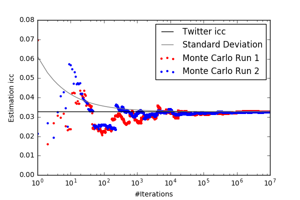
Experiments. We carried out two runs with 10 million iterations. It took about 2min30 for one run ($60.000$ iterations per second). The value of the estimator of the icc for the two runs is plotted as a function of the number of iterations in Figure 4. We first see that the estimator converges as expected to the value of the icc of TS represented by a straight horizontal line (and which was computed exactly in the previous section). We also plotted the estimated standard deviation as a function of the number of iterations. To obtain it, we did one billion iterations. We then estimated the standard deviation $\sigma$, and plotted $\frac{\sigma}{\sqrt{n}}$. We see that large jumps or discontinuity happen, but only at the beginning. They correspond to the draw of a fork with a lot of K22s and open K22s corresponding to a user who does not have the same icc as the global network. Then, the convergence is quick. After 300 iterations, the standard deviation is below 10% and after 1000 iterations, we do not experience a value of the runs less precise than 10%. .. [Fred: maybe give how many iterations for an average mistake of 10%, 1%…] Note that we have seen in Section 3.2 in Figures LABEL:fig:by-nodes/cc-distribution that nodes with very large numbers of K22s and open K22s, see Figures LABEL:fig:by-nodes/k22s-distribution. and LABEL:fig:by-nodes/openk22s-distribution.

$\begin{array}[]{|l|ccc|}\hline\cr&\#closed&\#open&cc\\ \hline\cr{\tt icc}&25,605,832,012,451,571&3,138,466,676,914,054,233&0.032634831\\ &2.610^{16}&3.110^{18}&3.3\%\\ tcc&2,469,018,039,988&129,023,573,841,024&0.019136178\\ &2.510^{12}&1.310^{14}&1.9\%\\ ccc&723,131,368,202&129,023,573,841,024&0.016813936\\ &7.210^{11}&1.310^{14}&1.7\%\\ ucc&623,873,346,660&1,631,948,600,661,523&0.001146862\\ &6.2310^{11}&1,6310^{15}&0.11\%\\ mcc&317,649,850,664&8,924,125,201,234&0.106783526\\ &3.210^{11}&8.910^{12}&10.7\%\\ \hline\cr\end{array}$

Table 1. Clustering coefficients (exact and approximated count) in the TS.

4. Results: Clustering coefficients in Twitter

To compute the number of K22s and open K22s, directed triangles, and undirected triangles in the Twitter Snapshot, we used a cluster with a rack of 16 Dell C6420 dual-Xeon 2.20GHz (20 cores), with $192\text{\,}\mathrm{G}\mathrm{B}$ RAM, all sharing an NFS Linux partition over Infiniband. It took 51 hours to compute the exact numbers of K22s and open K22s, corresponding to 265h of cumulative computation times on the cluster. We reported the results in Table 1.

Number of K22s and triangles. We see that the numbers of K22s and open K22s are huge, $2.6\text{\times}{10}^{16}$ and $3.1\text{\times}{10}^{18}$, respectively. It has to be compared with the number of triangles which are several orders of magnitude smaller: e.g., $2.5\text{\times}{10}^{12}$ and $1.3\text{\times}{10}^{14}$ for transitive triangles.

Clustering coefficient in the mutual graph. The mutual graph captures the friendship relationships in the social network. The mutual clustering coefficient thus is high ($mcc=10.7\%$), as cliques of friends are frequent in Twitter.

Clustering coefficients in the whole graph. We observe that ${\tt icc}=3.3\%>tcc=1.9\%>ccc=1.7\%>ucc=0.11\%$. Directed metrics better capture the interest relationships in the TS as ucc is very low. The highest parameter is the icc. It confirms the hypothesis of this paper that common interests between two users are better captured by the notion of K22 than by a direct link between these users. As expected, the second parameter is the one using transitive triangles. Indeed, they capture a natural way for a user of finding a new interesting user, that is, considering the followings of a following, especially after having seen retweets. A bit surprisingly, the ccc is not very low. In fact, a large fraction of the cyclic triangles are explained by corresponding triangles in the mutual graph (triangles of bi-directional links).
A way to artificially take off the social influence in order to focus exclusively on the directed interest part of the graph is to remove the (open and closed) triangles and K22s contained in the mutual graph from the total count. Indeed, each undirected triangle of the mutual graph induces two cyclic triangles and four transitive triangles, and each undirected open triangle induces two open triangles. In the same way, each undirected K22 induces two K22s and each undirected open K22 induces two open K22s. The obtained results are shown in Table 2. If we take off those mutual triangles, both the tcc and the ccc values drop to $0.51\%$ and $0.24\%$, respectively, while the icc stays about the same at $3.1\%$. This tends to confirm the hypothesis that the directed triangle clusterings somehow measure the friendship part of the TS more than the interest part.

We can even go one step further by computing the number of triangles in the graph in which all bidirectional edges have been removed. In that case, the $ccc$ drastically drops to 0 (we found no cyclic triangles without at least a bidirectional arc in the dataset!) while tcc and interest clustering coefficient stay almost the sames, 3.6 and 4.2 respectively. This confirms that cyclic triangles are artificially created by friendship relations and that the $ccc$ gives no information about the directed part of the graph.

$\begin{array}[]{|l|cccc|}\hline\cr&icc&tcc&ccc&ucc\\ \hline\cr Twitter&3.1\%&0.51\%&0.24\%&0.057\%\\ \hline\cr\end{array}$

Table 2. Clustering coefficients without the mutual structures.

Figure 5. Histogram of the distribution of the interest clustering coefficient over all users of the Twitter Snapshot. The vertical bars indicate the value of the glocal icc (3.3%) and the average value (7.7%) or local icc.

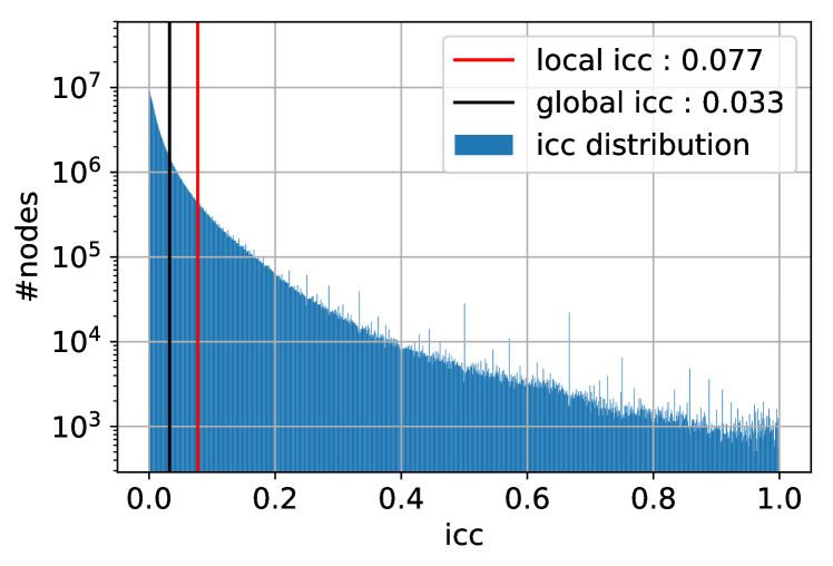
Distribution of the icc and local clustering. We also provide the distribution of the values of the interest clustering coefficient over all users (having open K22s) in Figure 5. We see that the icc greatly varies between 0 and 1. A large number of nodes have a low value of icc, e.g., $2.23\text{\times}{10}^{7}$ users ($10.2\%$ of the users with open K22s) have a value of 0, meaning they are part of open K22s but not of K22s. At the opposite end, $2.4\text{\times}{10}^{4}$ users ($0.011\%$ of the users with open K22s) have a value of 1, meaning that all their open K22s belong to a K22. The average value is equal to 7.7%. This value could be used as a definition of a local ${\tt icc}^{\top}$. Indeed, as discussed above, the number of K22s and open K22s per user have been computed while considering a user as a top vertex. A second local coefficient, ${\tt icc}_{\bot}$, can be defined for bottom vertices.
Similarly to what was found in Facebook, the local coefficient has a larger value than the global one. This may be due to the fact that a large number of nodes with few K22s and open K22s (usually nodes with small degrees) only are in a single small strongly connected community, and thus have a higher than average icc. On the contrary, a small number of nodes with larger degrees and larger number of K22s and open K22s may be in different communities, leading to smaller than average icc.

5. Results: Other Directed Datasets

	Is a Social Network	N	$|E|$	$\frac{|E|_{m}}{|E|}$
Instagram	Yes	$4.5\text{\times}{10}^{4}$	$6.7\text{\times}{10}^{5}$	11%
Flickr	Yes	$2.3\text{\times}{10}^{6}$	$3.3\text{\times}{10}^{7}$	62%
Web (.edu)	No	$6.9\text{\times}{10}^{5}$	$7.6\text{\times}{10}^{6}$	25%
Citations	No	$3.8\text{\times}{10}^{6}$	$1.7\text{\times}{10}^{7}$	0%

Table 3. Datasets information. $N$ is the number of nodes, $|E|$ the number of edges, and $\frac{|E|_{m}}{|E|}$ the fraction of edges implied in a bidirectional link.

	icc	tcc	ccc	mcc	ucc
Instagram	12.0%	15.4%	3.7%	22.6%	4.1%
Flickr	12.4%	12.2%	9.3%	13.9%	10.8%
Web (.edu)	46.3%	59.6%	18.8%	78.5%	0.69%
Citations	22.3%	9.1%	0%	(none)	6.7%

Table 4. Clustering coefficients of the directed datasets.

We computed the different metrics on four other directed networks: two social networks, a web networks and a citation network. The data information are gathered in Table 3, while the clustering coefficients are reported in Table 4. We also computed the values of the clustering coefficients without the mutual structures (not provided here); interestingly, those values are close to the ones on the total graphs.
We observe that the structure of each dataset is revealed by (the mix of) values of the different clustering coefficients, as discussed below.

Instagram: Instagram is a photo and video-sharing social network. This dataset was collected by Ferrara et al. (ferrara2014online, ) in 2014. The network is close to the Twitter one. Nodes corresponds to the accounts, and there is a link $u\rightarrow v$ if the account u follows the account v. The results are quite similar to what we found for Twitter: the $icc$ and $tcc$ are high and of the same order; the $ccc$ is also high because of the bidirectionnal edges (it drastically drops to 0.06% when removing those links). The $mcc$ is the highest value, while the $ucc$ is lower than the others. This confirms that social networks exhibit some common characteristics.

Flickr: Flickr is an image and video hosting service, which allows you to follow other people on the plateform to see more easily their content. The dataset was collected in 2008 by Mislove et al. (mislove-2008-flickr, ). This is once again a graph of followers of a directed social network. The values are similar to the previous one but for the $ucc$, which is higher. We can notice that Flickr looks more like a social media than Twitter and Instagram, since there is 62% of links implied in bidirectional. This explains why the undirected clustering coefficient is not so different from the mutual one .

Berkley-Stanford.edu web pages: The dataset was collected in 2002 by Leskovec et al.(leskovec2009community, ). The nodes represent the pages from berkely.edu and stanford.edu domains and directed edges represent hyperlinks between them. The $tcc$, $icc$, and $mcc$ are really high. For the $tcc$, this is due to the very hierarchical structure of the institution web pages. As an example, a researcher will be linking towards his group, laboratory, and university in its website, while the group website is linking to its laboratory and university… This strong structure translates into a high value of the $tcc$. As for the $icc$, research and educational domains form naturally strong communities creating large number of common neighbors for individuals of the same domain, and thus a high $icc$. Groups/teams/departments also constitutes strong social communities, leading to a high $mcc$.

Citations: Collected by Leskovec et al.(leskovec2005graphs, ), it includes all citations made by patents granted between 1975 and 1999. This is a good example of information network, giving a high value of icc of 22.6%, while the tcc value is 9.1%. Indeed, research fields and industry domains are strong communities leading to a high icc. Moreover, it is also not rare to cite a patent and its citations (the patent acting as a survey), explaining the tcc value. Note that there are no cyclic triangles nor bidirectional links, because of the temporal structure of citations - a paper will only cite older papers.

Takeaways: The following takeaways summarize the variety of informations given by the different clustering coefficients:

• A high value of icc indicates the presence of clusters of interests such as research communities or interest fields.

• A high value of tcc is the sign of an important local phenomena of friends’ or acquaintances’ recommendations and/or of a high hierarchical structure in the dataset.

• The ccc has no real social meaning. If its value can be high in a directed graph, this is only due to the presence of bidirectional arcs and triangles. The closure of a cyclic triangles is very rare in directed networks with no bidirectionnal edges, confirming the general intuition.

• Directed networks have a high $mcc$. Indeed, their bidirectional parts (mutual graph) have strong social communities, leading to a high clustering coefficient.

• The ucc is usually significantly lower, showing that the directed part of the network is better understood using directed clustering coefficients.

• Directed social networks have similar mixes of values of their undirected and directed clustering coefficients, however, with some notable differences, due to their diverse usages and information.

6. Model with addition of K22s

To model complex networks, a model with a high number of triangles was introduced in (vazquez2003growing, ). In this section, we introduce a new random graph model in which the number of K22s is higher than classical directed random graphs. The model is based on the model from Bollobás et al. (bollobas2003directed, ) to which we add what we call a K22 event. A K22 event closes an open K22. The principle is that if a user has a common interest with another user, and if this user has another interest, it has an increased chance to be interested and to follow it. We then show that the in-degree and out-degree distributions of the introduced model follow a power law (as many real networks). Lastly, we exhibit the increase of the interest clustering coefficient of the generated graphs with the probability of a K22 event.

6.1. Presentation of the model

We recall here the events defining the classic preferential attachment model of (bollobas2003directed, ) and define the K22 event. We start with an initial graph $G_{0}=(V_{0},E_{0})$. Then, at each time step t:

• With a probability (1-p) (Bollobás et al. event):

  • With a probability $\alpha$, we add a node u and a link leaving this node and reaching an existing node v chosen with a probability proportional to $d_{in}(v)+\delta_{in}$;

  • With a probability $\beta$, we add a node v and a link reaching this node and leaving an existing node u chosen with a probability proportional to $d_{out}(u)+\delta_{out}$;

  • With a probability $1-\alpha-\beta$, we add an edge between two existing nodes, chosen with probability proportional to $d_{out}(u)+\delta_{out}$ for the leaving node u and $d_{in}(v)+\delta_{in}$ for the reached node v.

• With a probability $p$ (K22 event):

  • We choose a random node (called $u_{1}$) with a probability proportional to its out-degree $d_{out}(u_{1})$;

  • We pick uniformly at random an out-neighbor of the node $u_{1}$ (called $v_{1}$);

  • We pick uniformly at random an in-neighbor of the node $v_{1}$ (called $u_{2}$);

  • We pick uniformly at random pick an out-neighbor of the node $u_{2}$ (called $v_{2}$);

  • We add a link from $u_{1}$ to $v_{2}$.

The idea of the K22 event is to close an open K22 ; since $u_{2}$ follows $v_{1}$ and $v_{2}$ at the same time, $v_{1}$ and $v_{2}$ have a higher probability to be similar, and a person $u_{1}$ following $v_{1}$ has a higher chance to be interested in $v_{2}$.
Note that it is possible to introduce multiedges with the K22 events. Indeed, to make the problem tractable, we allow $u_{1}=u_{2}$ in Step 3), or $v_{2}=v_{1}$ in Step 4). In the empirical study, we construct the random graphs with the multiedges and we get rid of them at the end of the constructions. We empirically verify that the multiedges do not impact the results in the end of the section. Indeed, most of them appear for low degree nodes and, thus, they do not affect the tail of the degree distributions.

Courbe du nb de multiedges en annexe en fonction de p et pour différents $\alpha$ ?

6.2. In-degree and out-degree distributions

We show in what follows that the in- and out-degree distributions of the introduced model follow power-laws, as most real networks. More precisely:

Theorem 6.1.

The probability $P(i)$ (resp. $P(o)$) for a node to have in-degree $i$ (resp. out-degree $o$) in the new model is:

$$P(i)\underset{i>>1}{\sim}i^{-(1+\frac{1}{A})}\quad\mbox{ and }\quad P(o)\underset{o>>1}{\sim}o^{-(1+\frac{1}{B})},$$

where $A=p+\frac{(1-p)(1-\beta)}{1+(1-p)(\alpha+\beta)\delta_{in}}$ and $B=p+\frac{(1-p)(1-\alpha)}{1+(1-p)(\alpha+\beta)\delta_{out}}$.

Proof.

We first focus on the in-degree distribution. This result is derived from the equation giving the evolution of the number of nodes of in-degree $i$ as a function of time, sometimes called Master Equation.
Let $G(t)=(V(t),E(t))$ be the graph obtained at time $t$, and $N(t)=|V(t)|$. The number of edges at time $t$ is $|E(t)|=t+|E_{0}|\approx t$, while the number of nodes is $N(t)=(1-p)(\alpha+\beta)(t+|V_{0}|)\approx(1-p)(\alpha+\beta)t$ when t is high enough. Hence, the mean in-degree (and out-degree) of the network is $m=\frac{1}{(1-p)(\alpha+\beta)}$.

Let us compute the in-degree distribution. Calling $N(i,t)$ the number of nodes of in-degree $i$ at time $t$, we can write the Master Equation:

$$N(i,t+1)-N(i,t)=(1-p)\alpha\delta_{0,i}+(1-p)\beta\delta_{1,i}$$

$$\mbox{ }+(1-p)(1-\beta)\frac{i-1+\delta_{in}}{\sum\limits_{i=0}^{+\infty}N(i,t)(i+\delta_{in})}N(i-1,t)$$

$$\mbox{ }-(1-p)(1-\beta)\frac{i+\delta_{in}}{\sum\limits_{i=0}^{+\infty}N(i,t)(i+\delta_{in})}N(i,t)$$

$$\mbox{ }+p\frac{i-1}{\sum\limits_{i=0}^{+\infty}N(i,t)i}N(i-1,t)-p\frac{i}{\sum\limits_{i=0}^{+\infty}N(i,t)i}N(i,t)$$

where $\delta_{i,j}$ is the Kronecker delta.
The Master Equation formulates the variation of the number of nodes with degree i between time $i$ and time $i+1$. The two first terms on the right hand side correspond to the addition of a new node, with degree 0 or 1 (depending on if we are in the first or second case of the Bollobás et al. event). The third and fourth terms are the probabilities that, during the Bollobás et al. event, an edge is connected to a node of degree $(i-1)$ or $i$. This would lead to the arrival of a new node of degree $i$, or the loss of one of them. Those events occur with probability $(1-p)(\alpha+(1-\alpha-\beta))$. Finally, the last two terms correspond to the probability that an edge connects a node of degree $(i-1)$ or $i$ during the K22 event.
We now show that the probability to connect to a node ($v_{2}$) of a given degree after following an open K22 is proportional to the degree of this node. Indeed, the probability to connect to a node ($v_{2}$) of a given degree after following an open K22 is

$$P(x=v_{2})=\sum\limits_{y\in N^{+}(v_{2})}P(y=u_{2})\times\frac{1}{d_{out}(y)},$$

where $N^{+}(v_{2})$ is the set of in-neighbors of $v_{2}$, and $u_{2}$ is defined in the model. Using the same reasoning, we have

$$P(x=u_{2})=\sum\limits_{y\in N^{-}(u_{2})}P(y=v_{1})\times\frac{1}{d_{in}(y)}$$

and

$$P(x=v_{1})=\sum\limits_{y\in N^{+}(v_{1})}P(y=u_{1})\times\frac{1}{d_{out}(y)}.$$

Since $P(y=u_{1})=\frac{d_{out}(y)}{t}$, we deduce that

$$P(x=v_{2})=\frac{d_{in}(x)}{t},$$

which gives us the expected result.

Using this property and knowing that

$$\sum\limits_{i=0}^{+\infty}i\cdot N(i,t)=|E(t)|=t$$

and

$$\sum\limits_{i=0}^{+\infty}N(i,t)\delta_{in}=\delta_{in}N(t)=(1-p)(\alpha+\beta)\delta_{in},$$

we can rewrite the equation as:

$$N(i,t+1)=\alpha\delta_{0,i}+\beta\delta_{1,i}$$

$$\mbox{ }+\Big{(}p\frac{i-1}{1}+(1-p)(1-\beta)\frac{i-1+\delta_{in}}{1+(1-p)(\alpha+\beta)\delta_{in}}\Big{)}\frac{N(i-1,t)}{t}$$

$$\mbox{ }-\Big{(}1+\big{(}p\frac{i}{1}+(1-p)(1-\beta)\frac{i+\delta_{in}}{1+(1-p)(\alpha+\beta)\delta_{in}}\big{)}\frac{1}{t}\Big{)}N(i,t).$$

Let us call

$$Z\equiv 1+(1-p)(\alpha+\beta)\delta_{in}.$$

We need the following lemma from (durrett2007random, ):

Lemma 6.2 ((durrett2007random, )).

If we have an equation of the form :

$$N(i,t+1)=\Big{(}1-\frac{b(t)}{t}\Big{)}N(i,t)+g(t)$$

where $b(t)\rightarrow b$ and $g(t)\rightarrow g$ as $t\rightarrow+\infty$, then

$$\frac{N(i,t)}{t}\rightarrow\frac{g}{b+1}.$$

Using Lemma 6.2 and calling $P(i)=\lim\limits_{t\rightarrow+\infty}\frac{N(i,t)}{t}$, we have:

$$P(i) =\frac{\big{(}\frac{(1-p)(1-\beta)}{Z}+p\big{)}(i-1)+\frac{\delta_{in}}{Z}}{1+\big{(}\frac{(1-p)(1-\beta)}{Z}+p\big{)}i+\frac{\delta_{in}}{Z}}P(i-1).$$

Let us call

$$A\equiv\frac{(1-p)(1-\beta)}{Z}+p.$$

We thus have:

$$P(i) =\frac{i-1+\frac{\delta_{in}}{ZA}}{i+\frac{\delta_{in}}{ZA}+\frac{1}{A}}P(i-1)$$

$$=P(1)\prod\limits_{k=2}^{i}\frac{k-1+\frac{\delta_{in}}{ZA}}{k+\frac{\delta_{in}}{ZA}+\frac{1}{A}}$$

$$=\frac{\Gamma(i+\frac{\delta_{in}}{ZA})\Gamma(\frac{1}{A}+\frac{\delta_{in}}{ZA}+2)}{\Gamma(i+\frac{\delta_{in}}{ZA}+\frac{1}{A}+1)\Gamma(\frac{\delta_{in}}{ZA}+1)}.$$

Leading to

$$P(i)\underset{i>>1}{\sim}i^{-(1+\frac{1}{A})}.$$

The out-degree distribution calculation follows the same method. The master equation is the same, except that $\delta_{in}$ and $\beta$ are replaced by $\delta_{out}$ and $\alpha$. The slope of the out-degree distribution is thus:

$$P_{out}(o)\underset{o>>1}{\sim}o^{-(1+\frac{1}{B})},\mbox{with }B=\frac{(1-p)(1-\alpha)}{1+(1-p)(\alpha+\beta)\delta_{out}}+p.$$

Concentration. We have studied here the mean of the distributions. We now use the Azuma’s inequalities to show the concentration around the mean. We have the following result (durrett2007random, ): Let $X_{t}$ be a martingale with $|X_{s}-X_{s-1}|\leq c$ for $1\leq s\leq t$. Then:

$$P(|X_{t}-X_{0}|>x)\leq\exp(-x^{2}/2c^{2}t).$$

Let $Z(i,t)$ be the number of vertices of degree $i$ at time $t$ and let $F_{s}$ denote the $\sigma$-field generated by the choices up to time $s$. We apply the result to $X_{s}=E(Z(i,t)|F_{s})$. We have that $|X_{s}-X_{s-1}|\leq 2$. Indeed, when we add an edge in the network, we affect only the degrees of its two end-vertices. Since $Z(i,0)=E(Z(i,t))$, using the result with $x=\sqrt{t\log(t)}$, we have

$$P(|Z(i,t)-E(Z(i,t))|>\sqrt{t\log(t)})\leq t^{-\frac{1}{8}}.$$

And hence, $\frac{Z(i,t)}{t}\underset{t\rightarrow+\infty}{\rightarrow}P(i)$ in probability. ∎

The degree distributions of the model follow power-laws, with exponents between $-2$ and $-\infty$. We notice that, for $p=0$, we recover the exponents of the Bollobás et al. model $-(1+\frac{1+(\alpha+\beta)\delta_{in}}{1-\beta})$ and $-(1+\frac{1+(\alpha+\beta)\delta_{out}}{1-\alpha})$ (bollobas2003directed, ), while, when $p$ goes to $1$, the exponent goes to $-2$.

Note that, similarly to the Bollobás et al. model, we cannot generate graphs with any wanted mean-degree and fixed slopes of the power-law. Some constraints exist in order to keep $\delta_{in}>0$ and $\delta_{out}>0$. For instance, with $\alpha=\beta=0.4$ and slopes of $-2.5$ (the values of our experiments), $p$ has to stay in the interval $[\frac{1}{6},\frac{2}{3}]$.

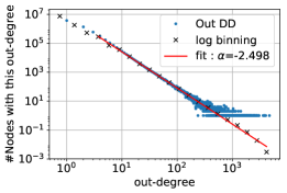
Validation by simulations. We validate the analysis and the hypothesis by simulation. In Figure 6, we present the in- and out-degree distributions of a network built with our new model as an example. The parameters are fixed to $p=0.5$, $\alpha=\beta=0.4$, and $\delta_{in}=\delta_{out}=2.0$. In this case, the expected slopes are $-2.5$. The fit is almost perfect: $-2.509$ and $-2.498$ for the in- and out-degree distributions.

Figure 6. In- (Top) and out- (Bottom) degree distributions of a network built with the new model. The obtained distribution is given by the blue points; the black crosses represent the logarithmic binning of the distribution (a mean of a given amount of points on a logarithmic scale). The red straight line is the fit of the logarithmic binning; it has slope of $-2.509$ (resp. $-2.498$) for the in- (resp. out-) degree distribution (expected slopes from analysis are $-2.5$).

6.3. Interest clustering coefficient of the new model

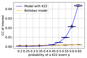
We show by simulation how the icc increases as $p$ increases. We compare it with the one of the Bollobás et al. model. Note that, when $p$ increases, the average degree of the model increases. Indeed, the mean degree is $m_{new}=\frac{1}{(1-p)(\alpha+\beta)}$. To compare networks with the same characteristics (mean degrees and exponents of the in-degree distribution), we adapt the parameters of the second model with the value of $p$.
Since, in the Bollobas et al. model, the mean degree is $m_{Bol}=\frac{1}{\alpha+\beta}$, we can compare the two models by: choosing the values of $\alpha$, $\beta$, and $p$ for our model. This imposes a value of $m$. We then choose $\alpha$, $\beta$ for the Bollobás et al. model, so that the two networks have the same mean degree. Finally, we choose $\delta_{in}$ so that the exponent of the in-degree distribution stays the same in both networks. In practice, we have fixed the exponent to $-2.5$ and imposed $\alpha_{new}=\beta_{new}=0.4$. We compare the icc for both models for different values of $p$ and report the results in Figure 7. We used graphs of size $N=10^{7}$ nodes and averaged over 10 networks for each point. We see that the icc varies from 0.036% to 4.4% when $p$ varies from 0.2 to 0.6.

Figure 7. Interest clustering coefficient of our new model as a function of $p$, the probability of a K22 event. The value is compared with the one of the Bollobás et al. model (bollobas2003directed, ).

7. Link Recommendation

[Fred: could we put the results for 1000 users?]

We propose to use the K22s defined for our metric to carry out link recommendation, as we advocate that the interest clustering coefficient is a good measure of common user interests. For a neighbor, the principle is to recommend links closing open K22s. We define the strength of a link as the number of open k22s it would close if added to the graph. Links are then recommended by decreasing strengths. Typical recommendation systems propose the strongest link to a user (e.g., Facebook) or a top 10/top 20 list (e.g., Youtube).

We tested our method on the Twitter snapshot. We considered a population of 1000 users selected uniformly at random over the full population of Twitter’s users. Note that we excluded users following no one. Indeed, isolated users are not interesting users per se and for this study and they have no TT or K22 recommendations.

For each node, we computed its open K22s (for a node $x$, we follow all its out-neighbors, then for each out-neighbor, we follow its in-neighbors, then for each in-neighbor, we follow its out-neighbors. These last nodes (which were not already followed by $x$) are the recommended nodes. We then count how many times a node is recommended. This gives the link strength.

We compared the method with classic recommendations using triangles. For example, on Facebook, it is frequent to have a message such as “8 of your friends know Bob. Do you know Bob?” Connecting with Bob would close 8 open (undirected) triangles. As we are considering a directed graph and are focusing on interest links, we computed recommendations based on transitive triangles, as they have more social sense than cyclic triangles. For a user $x$, we recommend the out-neighbors of the out-neighbors of $x$.

the nodes followed by the nodes that $x$ follows are recommended. We could have also studied undirected triangles. Future works?

Note that there are a lot more open K22s than open triangles in the graph, $3.1\text{\times}{10}^{18}$ compared to $1.3\text{\times}{10}^{14}$. We argue in the following that it allows to make more recommendations and most importantly better recommendations.

Figure 8. Cumulative distribution of the max and 10th recommendation strength over 1000 random Twitter’s users for K22 recommendation (Top) and transitive triangle recommendation (Bottom). The left plots are a zoom on recommendations with weak strengths ($\geq 20$). The right plots present the complete cumulative distribution in log scale. Beware of the y-scale for the K22 zoom left plot.

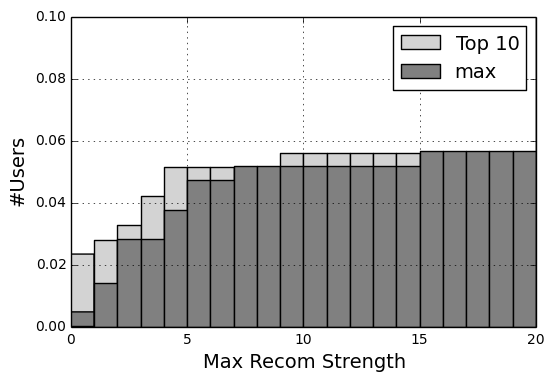
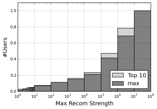
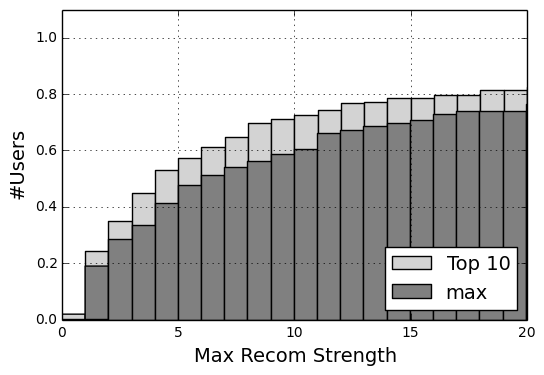
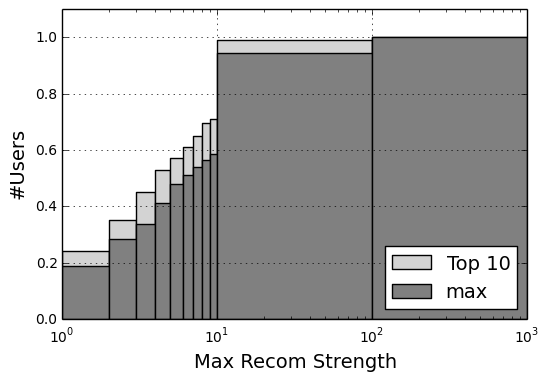
We report in Figure 8 histograms of the cumulative distribution over the 1000 random users of the strengths of the recommendation with maximum strength and of the 10th recommendation. The top plots present K22 recommendations while the bottom ones the TT recommendations. The right plots show the complete cumulative distribution in log scale, while the left plots are a zoom on recommendations with weak strengths ($\leq 20$). Beware that the y-scale of the K22 zoom left plot which is between 0 and 0.1. Notice also the difference in x-scale for the right plots.

Top/Max recommendation. We remark that a small amount of users have TT recommendations and no K22 recommendation. This is due to the fact that for a user with few outgoing links, it is more probable that the followed users are also following at least one other user (providing a TT recommendation) than they are followed by other users (necessary to provide a K22 recommendation). We do not advocate to use only K22 recommendations, but to use it as a complementary tool. In particular, for users with no TT and K22, recommendations would only be made based on global social network statistics (trending topics for example).

However, when a K22 recommendation exists for a user, it has much more strength than the TT recommendations for her. Indeed, 21% of users have TT recommendations of strengths 0 or 1. This number is just 1.2% for K22 recommendations. A recommendation of strength 1 has very good chance to be of no interest, as it is based on the following of a single user over 500 million ones. Similarly, 28% of users only have TT recommendations of strengths 2 or lower (to be compared with 2.5% for K22 recommendations). This means that, for a very large portion of users, TT recommendations are based on very few links. On the contrary, more than 94% of users have a top K22 recommendation with strength more than 10. We are thus able to carry out a meaningful recommendation for the vast majority of users using K22s.

Top 10 recommendations. When considering a recommendation system proposing a top 10, we see that 25% of users have their $10$th TT-recommendation of strength 1 or lower, and 35% of strength 2 or lower. There does not exist a significant top 10 list for more than one third of users. On the contrary, 94% of users have their $10$th K22-recommendation with strength higher than 10. Top 10 recommendation systems can thus be implemented for most users using K22s. Moreover, the distribution of recommendation strengths is very flat when using TT (a large number of top recommendations have strength 1), see Figure 9. Thus, it is very hard to discriminate between recommended users and to do a meaningful ranking of recommendations. At the opposite end, the distribution usually is steep for K22. It is thus a lot easier to establish a ranking.

Figure 9. Strengths of the top 10 recommendations for 2 typical Twitter users using (Left) K22 recommendations (Right) TT recommendations.

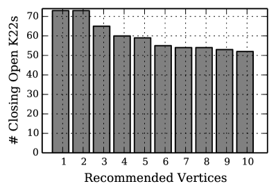
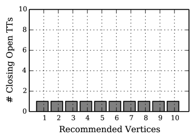
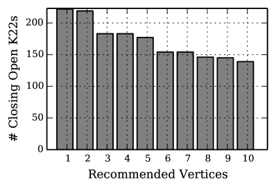
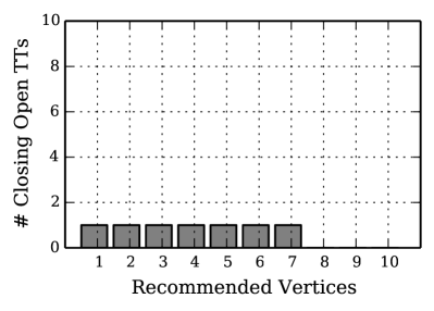
Typical users. We present in Figure 9 the strengths of the top 10 recommendations using K22 (Left) and TT (Right) for two typical users. For the first one (Top), it is implicated in around 200 triangles, representing each a potential recommendation. However, the strength of the recommendations is very low, just 1 for all of them. Recommendations for this user would be very bad for two reasons: first, they are based on the choice of only 1 user. Second, if the recommendation system had to propose a top 10, how would it discriminate between the 200 similar potential ones with similar strength. On the contrary, the K22 recommendations have much more strengths: 72 for the 1st and the 2d ones, and 52 for the 10th one. The K22 recommendations are thus much more well-grounded. For the second user (Bottom), we observe a similar phenomenon, but with fewer recommendations. It is not even possible to build a top 10 for her using TT as only 8 links can be proposed, and not with a high confidence (strength 1). Conversely, the top 10 K22 recommendations have strengths between 215 and 135.

The study should be dealt with more depth but we obtain some preliminary results:

• Some nodes with no classic triangle recommendation have K22 recommendations. We exhibit an example in Figure LABEL:fig:recommendations. In this case, recommendations would be only be made based on global social network statistics (trending topics for example). Using K22 recommendations thus would allow to make more personal recommendations than a recommend global recommendation.

• Note that there are more open K22s than open triangles in the graph $3.110^{18}$ compared to $1.310^{14}$. This allows to make more recommendations and (better) recommendations. To discuss more… When no triangle recommendation and more data when there are both (user 3)… A large average number per user, but it is really skewed…

• The reverse also happens. A node with no K22 recommendation which has triangle recommendations. We do not advocate to use only K22 recommendations, but to use it as a complementary tool.

• A large number of nodes do not have undirected mutual recommendations.

• Nodes recommended often differs.

Figure 10. FUTURE WORK? - Distribution of the number of K22s, open K22s and clustering coefficients per degree of users. Histogram and cdf. [Fred: curves do not make sense]

8. Conclusion

In this paper, we introduce a new metric, the interest clustering coefficient, to capture the interest phenomena in a directed graph. Indeed, the classical undirected clustering coefficient apprehends the social phenomena that my friends tend to be connected. However, it is not adequate to take into account directed interest links. The interest clustering coefficient is based on the idea that, if two people are following a common neighbor, they have a higher chance to have other common neighbors, since they have at least one interest in common. We computed this new metric on a network known to be at the same time a social and information media, a snapshot of Twitter from 2012 with 505 million users and 23 billion links. The computation was made on the total graph, giving the exact value of the interest clustering coefficient, and using sampling methods. The value of the interest clustering coefficient of Twitter is around 3.3%, higher than (undirected and directed) clustering coefficients introduced in the literature and based on triangles, which we also computed on the snapshot. This consolidates the idea that Twitter is indeed used as a social and information media, and that the new metric introduced in this paper captures the interest phenomena. We then proposed a new model, building random directed networks with a high value of K22s, and a new method for link recommendation using K22s. As a future work, we would like to investigate further link recommendation based on the K22 structure defined for the interest clustering coefficient: in particular, it would be interesting to carry out a real-world user case study to investigate if users are more satisfied by such recommendations.

References

- (1) Albert, R., Barabási, A.L.: Statistical mechanics of complex networks. Reviews of modern physics 74(1), 47 (2002)
- (2) Alon, N., Yuster, R., Zwick, U.: Finding and counting given length cycles. Algorithmica 17(3), 209–223 (1997)
- (3) Backstrom, L., Boldi, P., Rosa, M., Ugander, J., Vigna, S.: Four degrees of separation. In: Proceedings of the 4th Annual ACM Web Science Conference. pp. 33–42. ACM (2012)
- (4) Barrat, A., Weigt, M.: On the properties of small-world network models. The European Physical Journal B-Condensed Matter and Complex Systems 13(3), 547–560 (2000)
- (5) Bollobás, B., Borgs, C., Chayes, J., Riordan, O.: Directed scale-free graphs. In: Proceedings of the fourteenth annual ACM-SIAM symposium on Discrete algorithms. pp. 132–139. Society for Industrial and Applied Mathematics (2003)
- (6) Boykin, P.O., Roychowdhury, V.P.: Leveraging social networks to fight spam. Computer 38(4), 61–68 (2005)
- (7) Chen, J., Geyer, W., Dugan, C., Muller, M., Guy, I.: Make new friends, but keep the old: recommending people on social networking sites. In: Proceedings of the SIGCHI Conference on Human Factors in Computing Systems. pp. 201–210. ACM (2009)
- (8) Clauset, A., Shalizi, C.R., Newman, M.E.: Power-law distributions in empirical data. SIAM review 51(4), 661–703 (2009)
- (9) Coppersmith, D., Winograd, S.: Matrix multiplication via arithmetic progressions. In: Proceedings of the nineteenth annual ACM symposium on Theory of computing. pp. 1–6. ACM (1987)
- (10) Durrett, R.: Random graph dynamics, vol. 200. Cambridge university press Cambridge (2007)
- (11) Fagiolo, G.: Clustering in complex directed networks. Physical Review E 76(2), 026107 (2007)
- (12) Ferrara, E., Interdonato, R., Tagarelli, A.: Online popularity and topical interests through the lens of instagram. In: Proceedings of the 25th ACM conference on Hypertext and social media. pp. 24–34. ACM (2014)
- (13) Gabielkov, M., Legout, A.: The complete picture of the twitter social graph. In: Proceedings of the 2012 ACM conference on CoNEXT student workshop. pp. 19–20. ACM (2012)
- (14) Gabielkov, M., Rao, A., Legout, A.: Studying social networks at scale: macroscopic anatomy of the twitter social graph. In: ACM SIGMETRICS Performance Evaluation Review. vol. 42, pp. 277–288. ACM (2014)
- (15) Granovetter, M.S.: The strength of weak ties. In: Social networks, pp. 347–367. Elsevier (1977)
- (16) Kim, B.J.: Performance of networks of artificial neurons: The role of clustering. Physical Review E 69(4), 045101 (2004)
- (17) Kolountzakis, M.N., Miller, G.L., Peng, R., Tsourakakis, C.E.: Efficient triangle counting in large graphs via degree-based vertex partitioning. Internet Mathematics 8(1-2), 161–185 (2012)
- (18) Kwak, H., Lee, C., Park, H., Moon, S.: What is twitter, a social network or a news media? In: Proceedings of the 19th international conference on World wide web. pp. 591–600. ACM (2010)
- (19) Latapy, M.: Main-memory triangle computations for very large (sparse (power-law)) graphs. Theoretical Computer Science 407(1-3), 458–473 (2008)
- (20) Le Gall, F.: Powers of tensors and fast matrix multiplication. In: Proceedings of the 39th international symposium on symbolic and algebraic computation. pp. 296–303. ACM (2014)
- (21) Leskovec, J., Horvitz, E.: Planetary-scale views on a large instant-messaging network. In: Proceedings of the 17th international conference on World Wide Web. pp. 915–924. ACM (2008)
- (22) Leskovec, J., Kleinberg, J., Faloutsos, C.: Graphs over time: densification laws, shrinking diameters and possible explanations. In: Proceedings of the eleventh ACM SIGKDD international conference on Knowledge discovery in data mining. pp. 177–187. ACM (2005)
- (23) Leskovec, J., Lang, K.J., Dasgupta, A., Mahoney, M.W.: Community structure in large networks: Natural cluster sizes and the absence of large well-defined clusters. Internet Mathematics 6(1), 29–123 (2009)
- (24) Lü, L., Zhou, T.: Link prediction in complex networks: A survey. Physica A: statistical mechanics and its applications 390(6), 1150–1170 (2011)
- (25) Mislove, A., Koppula, H.S., Gummadi, K.P., Druschel, P., Bhattacharjee, B.: Growth of the flickr social network. In: Proceedings of the 1st ACM SIGCOMM Workshop on Social Networks (WOSN’08) (August 2008)
- (26) Mislove, A., Marcon, M., Gummadi, K.P., Druschel, P., Bhattacharjee, B.: Measurement and analysis of online social networks. In: Proceedings of the 7th ACM SIGCOMM conference on Internet measurement. pp. 29–42. ACM (2007)
- (27) Myers, S.A., Sharma, A., Gupta, P., Lin, J.: Information network or social network?: the structure of the twitter follow graph. In: Proceedings of the 23rd International Conference on World Wide Web. pp. 493–498. ACM (2014)
- (28) Newman, M.E.: Ego-centered networks and the ripple effect. Social Networks 25(1), 83–95 (2003)
- (29) Opsahl, T., Panzarasa, P.: Clustering in weighted networks. Social networks 31(2), 155–163 (2009)
- (30) Rossi, R., Ahmed, N.: The network data repository with interactive graph analytics and visualization. In: AAAI. vol. 15, pp. 4292–4293 (2015)
- (31) Sanei-Mehri, S.V., Sariyuce, A.E., Tirthapura, S.: Butterfly counting in bipartite networks. In: Proceedings of the 24th ACM SIGKDD International Conference on Knowledge Discovery & Data Mining. pp. 2150–2159. ACM (2018)
- (32) Saramäki, J., Kivelä, M., Onnela, J.P., Kaski, K., Kertesz, J.: Generalizations of the clustering coefficient to weighted complex networks. Physical Review E 75(2), 027105 (2007)
- (33) Schank, T., Wagner, D.: Finding, counting and listing all triangles in large graphs, an experimental study. In: International workshop on experimental and efficient algorithms. pp. 606–609. Springer (2005)
- (34) Shaban, H.: https://www.washingtonpost.com/technology/2019/02/07/twitter-reveals-its-daily-active-user-numbers-first-time/
- (35) Silva, N.B., Tsang, R., Cavalcanti, G.D., Tsang, J.: A graph-based friend recommendation system using genetic algorithm. In: Evolutionary Computation (CEC), 2010 IEEE Congress on. pp. 1–7. IEEE (2010)
- (36) Strogatz, S.H.: Exploring complex networks. nature 410(6825), 268 (2001)
- (37) Ugander, J., Karrer, B., Backstrom, L., Marlow, C.: The anatomy of the facebook social graph. arXiv preprint arXiv:1111.4503 (2011)
- (38) Vázquez, A.: Growing network with local rules: Preferential attachment, clustering hierarchy, and degree correlations. Physical Review E 67(5), 056104 (2003)
- (39) Wang, J., Fu, A.W.C., Cheng, J.: Rectangle counting in large bipartite graphs. In: 2014 IEEE International Congress on Big Data. pp. 17–24. IEEE (2014)
- (40) Watts, D.J., Strogatz, S.H.: Collective dynamics of ‘small-world’networks. nature 393(6684), 440 (1998)