Privacy-Aware Data Cleaning-as-a-Service

Abstract

Data cleaning is a pervasive problem for organizations as they try to reap value from their data. Recent advances in networking and cloud computing technology have fueled a new computing paradigm called Database-as-a-Service, where data management tasks are outsourced to large service providers. In this paper, we consider a Data Cleaning-as-a-Service model that allows a client to interact with a data cleaning provider who hosts curated, and sensitive data. We present PACAS: a Privacy-Aware data Cleaning-As-a-Service model that facilitates interaction between the parties with client query requests for data, and a service provider using a data pricing scheme that computes prices according to data sensitivity. We propose new extensions to the model to define generalized data repairs that obfuscate sensitive data to allow data sharing between the client and service provider. We present a new semantic distance measure to quantify the utility of such repairs, and we re-define the notion of consistency in the presence of generalized values. The PACAS model uses (X,Y,L)-anonymity that extends existing data publishing techniques to consider the semantics in the data while protecting sensitive values. Our evaluation over real data show that PACAS safeguards semantically related sensitive values, and provides lower repair errors compared to existing privacy-aware cleaning techniques.

1 Introduction

Data cleaning is a pervasive problem motivated by the fact that real data is rarely error free. Organizations continue to be hindered by poor data quality as they wrangle with their data to extract value. Recent studies estimate that up to 80% of the data analysis pipeline is consumed by data preparation tasks such as data cleaning [1]. A wealth of data cleaning solutions have been proposed to reduce this effort: constraint based cleaning that use dependencies as a benchmark to repair data values such that the data and dependencies are consistent [2], statistical based cleaning, which propose updates to the data according to expected statistical distributions [3], and leveraging master data as a source of ground truth [4].

Recent advances in networking and cloud infrastructure have motivated a new computing paradigm called Database-as-a-Service that lowers the cost and increases access to a suite of data management services. A service provider provides the necessary hardware and software platforms to support a variety of data management tasks to a client. Companies such as Amazon, Microsoft, and Google each provide storage platforms, accelerated computational capacity, and advanced data analytics services. However, the adoption of data cleaning services has been limited due to privacy restrictions that limit data sharing. Recent data cleaning efforts that use a curated, master data source share a similar service model to provide high quality data cleaning services to a client with inconsistent data [4, 5]. However, these techniques largely assume the master data is widely available, without differentiating information sensitivity among the attribute values.

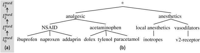
Figure 1: (a) ${\sf DGH}^{\sf med}$ and (b) ${\sf VGH}^{\sf med}$.

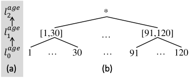
Figure 2: (a) ${\sf DGH}^{\sf age}$ and (b) ${\sf VGH}^{\sf age}$.

ID	GEN	AGE	ZIP	DIAG	MED
$m_{1}$	male	51	P0T2T0	osteoarthritis	ibuprofen
$m_{2}$	female	45	P2Y9L8	tendinitis	addaprin
$m_{3}$	female	32	P8R2S8	migraine	naproxen
$m_{4}$	female	67	V8D1S3	ulcer	tylenol
$m_{5}$	male	61	V1A4G1	migraine	dolex
$m_{6}$	male	79	V5H1K9	osteoarthritis	ibuprofen

Table 1: Curated medical records ($R_{SP}$)

ID	GEN	AGE	DIAG	MED
$t_{1}$	male	51	osteoarthritis	ibuprofen
$t_{2}$	male	79	osteoarthritis	intropes
$t_{3}$	male	45	osteoarthritis	addaprin
$t_{4}$	female	32	ulcer	naproxen
$t_{5}$	female	67	ulcer	tylenol
$t_{6}$	male	61	migrane	dolex
$t_{7}$	female	32	pylorospasm	appaprtin
$t_{8}$	male	37	hypertension	dolex

Table 2: Dirty client records w.r.t. $\varphi$.

ID	GEN	AGE	ZIP	DIAG	MED
$g_{1}$	*	[31,60]	P*	osteoarthritis	ibuprofen
$g_{2}$	*	[31,60]	P*	tendinitis	addaprin
$g_{3}$	*	[31,60]	P*	migraine	naproxen
$g_{4}$	*	[61,90]	V*	ulcer	tylenol
$g_{5}$	*	[61,90]	V*	migraine	dolex
$g_{6}$	*	[61,90]	V*	osteoarthritis	ibuprofen

Table 3: Public table.

Example 1.1

A data broker gathers longitudinal data from hospital and doctors’ records, prescription and insurance claims. Aggregating and curating these disparate datasets lead to a valuable commodity that clients are willing to pay for gleaned insights, and to enrich and clean their individual databases. Table 3 shows the curated data containing patient demographic, diagnosis and medication information. The schema consists of patient gender (GEN), age (AGE), zip code (ZIP), diagnosed illness (DIAG), and prescribed medication (MED).

A client such as a pharmaceutical firm, owns a stale and inconsistent subset of this data as shown in Table 3. For example, given a functional dependency (FD) $\varphi:[{\sf GEN},{\sf DIAG}]\rightarrow[{\sf MED}]$ on Table 3, it states that a person’s gender and diagnosed condition determine a prescribed medication. That is, for any two tuples in Table 3, if they share equal values in the [GEN, DIAG] attributes, then they should also have equal values in the MED attribute. We see that tuples ${t}_{1}$ - ${t}_{5}$ falsify $\varphi$. Error cells that violate $\varphi$ are highlighted in light and dark gray, and values in bold are inaccurate according to Table 3.

If the client wishes to clean her data with the help of a data cleaning service provider (i.e., the data broker and its data), she must first match the inconsistent records in Table 3 against the curated records in Table 3. This generates possible fixes (also known as repairs) to the data in Table 3. The preferred repair is to update $t_{2}[{\sf MED}]$, $t_{3}[{\sf MED}]$ to ibuprofen (from $m_{6}$), and $t_{4}[{\sf DIAG}]=$ migraine (from $m_{3}$). However, this repair discloses sensitive patient information about diagnosed illness and medication from the service provider. It may be preferable to disclose a more general value that is semantically similar to the true value to protect individual privacy. For example, instead of disclosing the medication ibuprofen, the service provider discloses Non-steroid anti-inflammatory drug (NSAID), which is the family of drugs containing ibuprofen. In this paper, we explore how to compute such generalized repairs in an interactive model between a service provider and a client to protect sensitive data and to improve accuracy and consistency in client data.

State-of-the-Art. Existing work in data privacy and data cleaning have been limited to imputation of missing values using decision trees [6], or information theoretic techniques [7], and studying trade-offs between privacy bounds and query accuracy over differentially private relations [8]. In the data cleaning-as-a-service setting, which we consider in this paper, using differential privacy poses the following limitations: (i) differential privacy provides guarantees assuming a limited number of interactions between the client and service provider; (ii) queries are limited to aggregation queries; and (iii) data randomization decreases data utility.

Given the above limitations, we explore the use of Privacy Preserving Data Publishing (PPDP) techniques, that even though do not provide the same provable privacy guarantees as differential privacy, do restrict the disclosure of sensitive values without limiting the types of queries nor the number of interactions between the client and service provider. PPDP models prevent re-identification and break attribute linkages in a published dataset by hiding an individual record among a group of other individuals. This is done by removing identifiers and generalizing quasi-identifier (QI) attributes (e.g., GEN, AGE, ZIP) that together can re-identify an individual. Well-known PPDP methods such as $k$-anonymity require the group size to be at least $k$ such that an individual cannot be identified from $k-1$ other individuals [9, 10]. Extensions include (X,Y)-anonymity that break the linkage between the set $X$ of QI attributes, and the set $Y$ of sensitive attributes by requiring at least $k$ distinct sensitive values for each unique $X$ [11]. For example, Table 3 is $k$-anonymous for $k=3$ by generalizing values in the QI attributes. It is also (X,Y)-anonymous for sensitive attribute MED for $k=3$ since there are three distinct medications for each value in the QI attributes $X$, e.g., values $(*,[31,60],P*)$ of $X$ co-occur with ibuprofen, addaprin, and naproxen of $Y$.

To apply PPDP models in data cleaning, we must also address the highly contextualized nature of data cleaning, where domain expertise is often needed to interpret the data to achieve correct results. It is vital to incorporate these domain semantics during the cleaning process, and into a privacy model during privacy preservation. Unfortunately existing PPDP models only consider syntactic forms of privacy via generalization and suppression of values, largely ignoring the data semantics. For example, upon closer inspection of Table 3, the values in the QI attributes in records $g_{1}-g_{3}$ are associated with the same family of medication, since ibuprofen, addaprin, and naproxen all belong to the the NSAID class, which are analgesic drugs. In past work, we introduced a privacy-preserving framework that uses an extension of (X,Y)-anonymity to incorporate a generalization hierarchy, which capture the semantics of an attribute domain [12]. In Table 3, the medications in $g_{1}-g_{3}$ are modeled as synonyms in such a hierarchy. In this paper, we extend our earlier work [12] to define a semantic distance metric between values in a generalization hierarchy, and to incorporate generalized values as part of the data repair process.

Example 1.2

To clean Table 3, a client requests the correct value(s) in tuples $t_{1}-t_{3}$ from the data cleaning service provider. The service provider returns ibuprofen to the client to update $t_{2}[{\sf MED}]$ and $t_{3}[{\sf MED}]$ to $m_{6}[{\sf MED}]=$ ibuprofen. However, disclosing the specific ibuprofen medication violates the requirements of the underlying privacy model. Hence, the service provider must determine when such cases arise, and offer a revised solution to disclose a less informative, generalized value, such as NSAID or analgesic. The model must provide a mechanism for the client and service provider to negotiate such a trade-off between data utility and data privacy.

Technical Challenges.

1. Data cleaning with functional dependencies (FDs), and record matching (between the service provider and client) is an NP-complete problem. In addition, it is approximation-hard, i.e., the problem cannot be approximately solved with a polynomial-time algorithm and a constant approximation ratio [4]. We extend this data cleaning problem with privacy restrictions on the service provider, making it as hard as the initial problem. In our earlier work, we analyzed the complexity of this problem, and proposed a data cleaning framework realizable in practice [12]. In this paper, we extend this framework to consider a new type of repair with generalized values that further protects sensitive data values.

2. Given a generalization hierarchy as shown in Figures 1 and 2, proposed repairs from a service provider may contain general values that subsume a set of specific values at the leaf level. In such cases, we study and propose a new (repair) semantics for data consistency with respect to (w.r.t.) an FD involving general values.

3. By proposing generalized values as repair values, we lose specificity in the client data instance. We study the trade-off between generalized versus specific repair values. Resolving inconsistencies w.r.t. a set of FDs requires traversing the space of possible fixes (which may now include general values). Quantifying the individual utility of a generalized value as a repair value, while respecting data cleaning budgets from the client is our third challenge.

Our Approach and Contributions. We build upon our earlier work that introduced PACAS, a $P$rivacy-$A$ware data $C$leaning-$A$s-a-$S$ervice framework that facilitates data cleaning between a client and a service provider [12]. The interaction is done via a data pricing scheme where the service provider charges the client for each disclosed value, according to its adherence to the privacy model. PACAS includes a new privacy model that extends (X,Y)-anonymity to consider the data semantics, while providing stronger privacy protection than existing PPDP methods. In this work, we present extensions to PACAS to resolve errors (FD violations) by permitting updates to the data that are generalizations of the true value to avoid disclosing details about sensitive values. Our goal is to provide repair recommendations that are semantically equivalent to the true value in the service provider data. We make the following contributions:

1. We extend PACAS  the existing privacy-preserving, data cleaning framework that identifies FD errors in client data, and allows the client to purchase clean, curated data from a service provider [12]. We extend the repair semantics to introduce generalized repairs that update values in the client instance to generalized values.

2. We re-define the notion of consistency between a relational instance (with generalized values) and a set of FDs. We propose an entropy-based measure that quantifies the semantic distance between two values to evaluate the utility of repair candidates.

3. We extend our SafeClean algorithm that resolves FD errors by using external data purchased from a service provider. SafeClean proposes repairs to the data by balancing its data privacy requirements against satisfying query purchase requests for its data at a computed price [12]. Given a cleaning budget, we present a new budget allocation algorithm that improves upon previous, fixed allocations, to consider allocations according to the number of errors in which a database value participates.

4. We evaluate the effectiveness of SafePrice and SafeClean over real data showing that by controlling data disclosure via data pricing, we can effectively repair FD violations while guaranteeing (X,Y,L)-anonymity. We also show that our SafeClean achieves lower repair error than comparative baseline techniques.

We provide notation and preliminaries in Section 2. In Section 3, we define generalized relations, and their consistency w.r.t. a set of FDs, and present a new semantic distance function. We present our problem definition, and review the PACAS system in Section 4. We discuss how data privacy is enforced via data pricing in Section 5, and describe new extensions to our data cleaning algorithm that consider generalized values in Section 6. We present our experimental results in Section 7, related work in Section 8, and conclude in Section 9.

2 Preliminaries

2.1 Relations and Dependencies

A relation (table) $R$ with a schema $\mathcal{R}=\{A_{1},...,A_{n}\}$ is a finite set of $n$-ary tuples $\{{t}_{1},...,{t}_{N}\}$. A database (instance) $D$ is a finite set of relations $R_{1},...,R_{m}$ with schema ${\color[rgb]{0,0,0}\mathfrak{R}}=\{\mathcal{R}_{1},...\mathcal{R}_{m}\}$. We denote by small letters $x,y,z$ as variables. Let $A,B,C$ refer to single attributes and $X,Y,Z$ as sets of attributes. A cell $c=t[A_{i}]$ is the $i$-th position in tuple ${t}$ with its value denoted by $c.{\sf value}$. We use $c$ to refer to the value $c.{\sf value}$ if it is clear from the context. A functional dependency (FD) $\varphi$ over a relation $R$ with set of attributes $\mathcal{R}$ is denoted by $\varphi:X\rightarrow Y$, in which $X$ and $Y$ are subsets of $\mathcal{R}$. We say $\varphi$ holds over $R$, $R\models\varphi$, if for every pair of tuples ${t}_{1}$, ${t}_{2}$ $\in R$, ${t}_{1}[X]={t}_{2}[X]$ implies ${t}_{1}[Y]={t}_{2}[Y]$. Table 4 summarizes our symbols and notations.

A matching dependency (MD) $\phi$ over two relations $R$ and $R^{\prime}$ with schemata $\mathcal{R}=\{A_{1},A_{2},...\}$ and $\mathcal{R}^{\prime}=\{A^{\prime}_{1},A^{\prime}_{2},...\}$ is an expression of the following form:

$$\bigwedge_{i\in[1,n]}R[X_{i}]\approx R^{\prime}[X^{\prime}_{i}]\rightarrow R[Y]\leftrightharpoons R^{\prime}[Y^{\prime}],$$ (1)

where $(X_{i},X^{\prime}_{i})$ and $(Y,Y^{\prime})$ are comparable pairs of attributes in $R$ and $R^{\prime}$. The MD $\phi$ states that for a pair of tuples $(t,t^{\prime})$ with $t\in R$ and $t^{\prime}\in R^{\prime}$, if $t[X^{\prime}_{i}]$ values are similar to values $t^{\prime}[X^{\prime}_{i}]$ according to the similarity function $\approx$, the values of $t[Y]$ and $t^{\prime}[Y^{\prime}]$ are identical [5].

Table 4: Summary of notation and symbols.

Symbol	Description
$R,\mathcal{R}$	relation and relational schema
$A,B$	relational attributes
$X,Y,Z$	sets of relational attributes
$D,{\color[rgb]{0,0,0}\mathfrak{R}}$	database instance and database schema
$\varphi,\phi$	functional dependency and matching dependency
${\sf Dom}^{A},{\sf dom}^{A}$	domain of attribute $A$
${\sf dom}^{A}(l)$	sub-domain of attribute $A$ in level $l$
${\sf DGH}^{A}$,${\sf VGH}^{A}$	domain and value generalization hierarchies
$\leq$	generalization relation for levels
$\preceq$	generalization relation for values, tuples, and relations
$Q,G$	Simple query and generalized query (GQ)
$l,L$	level and sequence of levels
$\mathcal{S},\mathcal{C}^{Q}$	support set, and conflict set
$\mathcal{B},B_{i}$	total and the budget for the i-th iteration
$l_{\sf max}$	generalization level
$c,e$	database cell and error cell
$\delta$	distance function for values, tuples and relations

2.2 Generalization

Generalization replaces values in a private table with less specific, but semantically consistent values according to a generalization hierarchy. To generalize attribute $A$, we assume a set of levels $\mathcal{L}^{A}=\{l^{A}_{0},...,l^{A}_{h}\}$ and a partial order $\leq^{A}$, called a generalization relation on $\mathcal{L}^{A}$. Levels $l^{A}_{i}$ are assigned with disjoint domain-sets ${\sf dom}(l^{A}_{i})$. In $\leq^{A}$, each level has at most one parent. The domain-set ${\sf dom}(l^{A}_{n})$ is the maximal domain set and it is a singleton, and ${\sf dom}(l^{A}_{0})$ is the ground domain set. The definition of $\leq^{A}$ implies the existence of a totally ordered hierarchy, called the domain generalization hierarchy, ${\sf DGH}^{A}$. The domain set ${\sf dom}(l^{A}_{i})$ generalizes ${\sf dom}(l^{A}_{j})$ iff $l^{A}_{j}\leq l^{A}_{i}$. We use $h^{A}$ to refer to the number of levels in ${\sf DGH}^{A}$. Figures 1(a) and 2(a) show the DGH s for the medication and age attributes, resp. A value generalization relationship for $A$, is a partial order $\preceq^{A}$ on ${\sf Dom}^{A}=\bigcup{\sf dom}(l^{A}_{i})$. It specifies a value generalization hierarchy, ${\sf VGH}^{A}$, that is a tree whose leaves are values of the ground domain-set ${\sf dom}(l^{A}_{0})$ and whose root is the single value in the maximal domain-set ${\sf dom}(l^{A}_{n})$ in ${\sf DGH}^{A}$. For two values $v$ and $v^{\prime}$ in ${\sf Dom}^{A}$, $v^{\prime}\preceq^{A}v$ means $v^{\prime}$ is more specific than $v$ according to the VGH. We use $\preceq$ rather than $\preceq^{A}$ when the attribute is clear from the context. The VGH for the MED and AGE attributes are shown in Figures  1(b) and 2(b), respectively. According to VGH of MED, ibuprofen $\preceq$ NSAID.

A value is ground if there is no value more specific than it, and it is general if it is not ground. In Figure 1, ibuprofen is ground and analgesic is general. For a value $v$, its base denoted by ${\sf base}(v)$ is the set of ground values $u$ such that $u\preceq v$. We use $0\leq{\sf level}(v)\leq h^{A}$ to refer to the level of $v$ according to ${\sf VGH}^{A}$.

A general relation (table) is a relation with some general values and a ground relation has only ground values. A general database is a database with some general relations and a ground database has only ground relations. The generalization relation $\preceq^{A}$ trivially extends to tuples. We give an extension of the generalization relation to general relations and databases in Section 3.

The generalization hierarchies (DGH and VGH) are either created by the data owners with help from domain experts or generated automatically based on data characteristics [13]. The automatic generation of hierarchies for categorical attributes [14] and numerical attributes [15, 16, 17] apply techniques such as histogram construction, binning, numeric clustering, and entropy-based discretization [13].

2.3 Generalized Queries

We review generalized queries (GQs) to access values at different levels of the DGH [12].

Definition 1 (Generalized Queries)

A generalized query (GQ) with schema $\mathcal{R}$ is a pair $G=\langle Q,L\rangle$, where $Q$ is an $n$-ary select-projection-join query over $\mathcal{R}$, and $L=\{l_{1},...,l_{n}\}$ is a set of levels for each of the $n$ values in $Q$ according to the DGHs in $\mathcal{R}$. The set of answers to $G$ over $R$, denoted as $G(R)$, contains $n$-ary tuples ${t}$ with values at levels in $l_{i}\in{\sf L}$, such that $\exists{t}^{\prime}\in Q(R)$ and ${t}$ generalizes ${t}^{\prime}$, i.e. ${t}^{\prime}\preceq{t}$.

Intuitively, answering a GQ involves finding the answers of $Q(R)$, and then generalizing these values to levels that match $L$. For a fixed size DGH, the complexity of answering $G$ is the same as answering $Q$.

Example 2.1

Consider a GQ $G=\langle Q,L\rangle$ with level $L=\{l_{0}^{\sf GEN}$, $l_{1}^{\sf MED}\}$ and query $Q(R_{SP})$ $=$ $\Pi_{\sf GEN,MED}(\sigma_{{\sf DIAG}={\sl migraine}}(R_{SP}))$ posed on relation $R_{SP}$ is Table 3. The query $Q$ requests the gender and medication of patients with a migraine. The answers to $Q(R_{SP})$ are {(female, naproxen), (male, dolex)}. The GQ $G$ asks for the same answers but at the levels specified by $L$. Therefore the answers to $G$ are {(female, NSAID), (male, acetaminophen)}, which are generalized according to $L$ and Figure 1.

2.4 Privacy-Preserving Data Publishing

The most well-known PPDP privacy model is $k$-anonymity that prevents re-identification of a single individual in an anonymized data set [9, 10].

Definition 2 ($X$-group and $k$-anonymity)

A relation $R$ is $k$-anonymous if every QI-group has at least $k$ tuples. An $X$-group is a set of tuples with the same values in $X$.

As an example, Table 3 has two QI-groups, $\{g_{1},g_{2},g_{3}\}$ and $\{g_{4},g_{5},g_{6}\}$, and it is $k$-anonymous with $k=3$. $k$-anonymity is known to be prone to attribute linkage attacks where an adversary can infer sensitive values given QI values. Techniques such as (X,Y)-anonymity aim to address this weakness by ensuring that for each QI value in $X$, there are at least $k$ different values of sensitive values in attribute(s) $Y$ in the published (public) data [18].

Definition 3 ((X,Y)-anonymity)

A table $R$ with schema $\mathcal{R}$ and attributes $X,Y\subseteq\mathcal{R}$ is (X,Y)-anonymous with value $k$ if for every ${t}\in R$, there are at least $k$ values in ${Q}^{t}(R)$, $|{Q}^{t}(R)|\geq k$, where ${Q}^{t}(R)=\Pi_{Y}(\sigma_{X=t[X]}(R))$.

The query $Q^{t}(R)$ in Definition 3 returns distinct values of attributes $Y$ that appear in $R$ with the values $t[X]$. Therefore, if the size of $Q^{t}(R)$ is greater than $k$ for every tuple $t$, that means every values of $X$ are linked with at least $k$ values of $Y$. Note that $k$-anonymity is a special case of (X,Y)-anonyity when $X$ is the set of QI attributes and $Y$ is the set of sensitive attributes that are also a key in $R$ [18].

Example 2.2

For $X=\{{\sf GEN},{\sf AGE},{\sf ZIP}\}$, $Y=\{{\sf MED}\}$ with $k=3$, Table 3 is (X,Y)-anonymous since each $g_{i}\in R$, ${Q}^{g_{i}}(R)$ is either {ibuprofen, addaprin, naproxen} or {tylenol, dolex, ibuprofen}, which means the values of $X$ in each tuple $g_{i}$ are linked to $k=3$ distinct values of $Y$ ($Q^{g_{i}}(R)$ represents the set of distinct values of $Y$ that are linked to the values of $g_{i}[X]$ in $R$). Table 3 is not (X,Y)-anonymous with $X=\{{\sf DIAG}\}$ and $Y=\{{\sf MED}\}$, since for $g_{1}$, ${Q}^{g_{1}}(R)=\{$ibuprofen$\}$ with size $1\leq k$.

The (X,Y)-anonymity model extends $k$-anonymity; if $Y$ is a key for $R$ and $X,Y$ are QI and sensitive attributes, respectively, then (X,Y)-anonymity reduces to $k$-anonymity.

The $l$-diversity privacy model extends $k$-anonymity with a stronger restriction over the $X$-groups [19]. A relation is considered $l$-diverse if each $X$-group contains at least $l$ “well-represented” values in the sensitive attributes $Y$. Well-representation is normally defined according to the application semantics, e.g., entropy $l$-diversity requires the entropy of sensitive values in each $X$-group to satisfy a given threshold [19]. When well-representation requires $l$ sensitive values in each $Y$ attribute, (X,Y)-anonymity reduces to $l$-diversity.

2.4.1 (X,Y,L)-anonymity.

In earlier work, we introduced (X,Y,L)-anonymity, which extends (X,Y)-anonymity to consider the semantic closeness of values [12]. Consider the following example showing the limitations of (X,Y)-anonymity.

Example 2.3

(X,Y)-anonymity prevents the linkage between sets of attributes $X$ and $Y$ in a relation $R$ by making sure that every values of $Y$ appears with at least $k$ distinct values of $X$ in $R$. For example, Table 3 is (X,Y)-anonymous with $X=\{{\sf GEN},{\sf AGE},{\sf ZIP}\}$, $Y=\{{\sf MED}\}$, and $k=3$ because the values of $X$ appear with three different values; $(*,[31,60],P*)$ co-occurs with ibuprofen, addaprin, naproxen and $(*,[61,90],V*)$ appears with tylenol, dolex, ibuprofen.

(X,Y)-anonymity ignores how close the values of $Y$ are according to their VGHs. For example, although ibuprofen, addaprin, naproxen are distinct values, they are similar medications with the same parent NSAID according to the VGH in Figure 1. This means the value $(*,[31,60],P*)$ of attributes $X$ is linked to NSAID which defies the purpose of (X,Y)-anonymity.

(X,Y,L)-anonymity resolves this issue by adding a new parameter $L$ for levels of $Y$. In (X,Y,L)-anonymity, every values of $X$ has to appear with at least $k$ values of $Y$ in the levels of $L$. For example, Table 3 is not (X,Y,L)-anonymous if $L=\{l_{1}^{\sf MED}\}$ because $(*,[31,60],P*)$ appears with $Y$ values that all roll up to NSAID at level $l_{1}^{\sf MED}$. Thus, to achieve (X,Y,L)-anonymity we need to further suppress values in Table 3 to prevent the linkage between $(*,[31,60],P*)$ and NSAID.

Definition 4 ((X,Y,L)-anonymity)

Consider a table $R$ with schema $\mathcal{R}$ and attributes $X,Y\subseteq\mathcal{R}$, and a set of levels $L$ corresponding to attribute DGHs from $Y$. $R$ is (X,Y,L)-anonymous with value $k$ if for every $t\in R$, there are at least $k$ values in ${G}^{t}(R)$, where ${G}^{t}=\langle{Q}^{t},L\rangle$ is a GQ with ${Q}^{t}(R)=\Pi_{Y}(\sigma_{X=t[X]}(R))$.

In Definition 4, the GQ $G^{t}(R)$ returns the set of $Y$ values in levels $L$ that appear with the $X$ values of the tuples $t$. If the size of $G^{t}(R)$ is greater than $k$, then every value of $X$ appears with at least $k$ values of $Y$ in the level $L$, which is the objective of (X,Y,L)-anonymity, as shown in Example 2.3.

2.5 Data Pricing

High quality data is a valuable commodity that has lead to increased purchasing and selling of data online. Data market services provide data across different domains such as geographic and locational (e.g., AggData [20]), advertising (e.g., Oracle [21], Acxiom [22]), social networking (e.g., Facebook [23], Twitter [24]), and people search (e.g. Spokeo [25]). These vendors have become popular in recent years, and query pricing has been proposed as a fine-grained and user-centric technique to support the exchange and marketing of data [26].

Given a database instance $D$ and query $Q$, a pricing function returns a non-negative real number representing the price to answer $Q$ [26]. A pricing function should have the desirable property of being arbitrage-free [26]. Arbitrage is defined using the concept of query determinacy [27]. Intuitively, $Q$ determines $Q^{\prime}$ if for every database $D$, the answers to $Q^{\prime}$ over $D$ can be computed from the answers to $Q$ over $D$. Arbitrage occurs when the price of $Q$ is less than that of $Q^{\prime}$, which means someone interested in purchasing $Q^{\prime}$ can purchase the cheaper $Q$ instead, and compute the answer to $Q^{\prime}$ from $Q$. For example, $Q(R)=\Pi_{Y}(R)$ determines $Q^{\prime}(R)=\Pi_{Y}(\sigma_{Y<10}(R))$ because the user can apply $Y<10$ over $Q(R)$ to obtain $Q^{\prime}(R)$. Arbitrage occurs if $Q$ is cheaper than $Q^{\prime}$ which means a user looking for $Q^{\prime}(R)$ can buy $Q$ and compute answers to $Q^{\prime}$. An arbitrage-free pricing function denies any form of arbitrage and returns consistent pricing without inadvertent data leakage [26]. A pricing scheme should also be history-aware [26]. A user should not be charged multiple times for the same data purchased through different queries. In such a pricing scheme, the data seller must track the history of queries purchased by each buyer and price future queries according to historical data.

3 Generalized Relations

Using general values as repair values in data cleaning requires us to re-consider the definition of consistency between a relational instance and a set of FDs. In this section, we introduce an entropy-based measure that allows us to quantify the utility of a generalized value as a repair value, and present a revised definition of consistency that has not been considered in past work [12].

3.1 Measuring Semantic Distance

By replacing a value $v^{\prime}$ in a relation $R$ with a generalized value $v$, there is necessarily some information loss. We present an entropy-based penalty function that quantifies this loss [28]. We then use this measure as a basis to define a distance function between two general values.

Definition 5 (Entropy-based Penalty [28])

Consider an attribute $A$ in a ground relation $R$. Let $X_{A}$ be a random variable to randomly select a value from attribute $A$ in $R$. Let ${\sf VGH}^{A}$ be the value generalization hierarchy of the attribute $A$ (the values of $A$ in $R$ are ground values from ${\sf VGH}^{A}$). The entropy-based penalty of a value $v$ in ${\sf VGH}^{A}$ denoted by $E(v)$ is defined as follows:

$$E(v)=P(X_{A}\in\textit{base}(v))\times H(X_{A}|X_{A}\in\textit{base}(v)),$$

where $P(X_{A}\in\textit{base}(v))$ is the probability that the value of $X_{A}$ is a ground value and a descendant of $v$, $X_{A}\in\textit{base}(v))$. The value $H(X_{A}|X_{A}\in\textit{base}(v))$ is the entropy of $X_{A}$ conditional to $X_{A}\in\textit{base}(v)$.

Intuitively, the entropy $H(X_{A}|X_{A}\in\textit{base}(v))$ measures the uncertainty of using the general value $v$. $E(v)$ measures the information loss of replacing values in $\textit{base}(v)$ with $v$. Note that $E(v)=0$ if $v$ is ground because $H(X_{A}|X_{A}\in\textit{base}(v))=0$, and $E(v)$ is maximum if $v$ is the root value $*$ in ${\sf VGH}^{A}$. $E(v)$ is monotonic whereby if $v\preceq v^{\prime}$, then $E(v)\leq E(v^{\prime})$. Note that the conditional entropy $H(X_{A}|X_{A}\in\textit{base}(v))$ is not a monotonic measure [28].

Example 3.1

Consider the general value $v=g_{1}[{\sf AGE}]=$[31,60] in Table 3. Three ground values 51, 45 and 32 in $base(v)$ appear in Table 3, which has total $6$ records, so $P(X_{\sf AGE}\in base(v))=\frac{3}{6}=\frac{1}{2}$. According to Table 3, the conditional entropy is $H(X_{A}|X_{\sf AGE}\in base(v))=3\times(-\frac{1}{3}\times\log\frac{1}{3})=1.58$ because 51, 45 and 32 each appear exactly once in the table. Therefore, the entropy-based penalty of $v$ is $E(v)=\frac{1}{2}\times 1.58=0.79$.

Definition 6 (Semantic Distance Function, $\delta$)

The semantic distance between $v$ and $v^{\prime}$ in ${\sf VGH}^{A}$ is defined as follows:

$$\delta(v,v^{\prime})=\begin{cases}|E(v^{\prime})-E(v)|&\textit{if}\;v\preceq v^{\prime}\;\textit{or}\;v^{\prime}\preceq v\\ \delta(v,a)+\delta(a,v^{\prime})&\textit{otherwise}\end{cases}$$

in which $a=\textit{lca}(v,v^{\prime})$ is the least common ancestor of $v$ and $v^{\prime}$.

Intuitively, if $v$ is a descendant of $v^{\prime}$ or vice versa, i.e. $v\preceq v^{\prime}$ or $v^{\prime}\preceq v$, their distance is the the difference between their entropy-based penalties, i.e., $|E(v^{\prime})-E(v)|$. This is the information loss incurred by replacing a more informative child value $v$ with its ancestor $v^{\prime}$ when $v\preceq v^{\prime}$. If $v$ and $v^{\prime}$ do not align along the same branch in the VGH, i.e. $v\not\preceq v^{\prime}$ and $v^{\prime}\not\preceq v$, $\delta(v,v^{\prime})$ is the total distance between $v$ and $v^{\prime}$ as we travel through their least common ancestor $a$, i.e. $\delta(v,a)+\delta(a,v^{\prime})$.

Example 3.2

(Ex. 3.1 continued) According to Definition 6, $\delta([31,60],51)=|E([31,60])-E(51)|=|0.79-0|=0.79$ because $51\preceq[31,60]$. Similarly, $\delta([31,60],45)=0.79$. Also, $\delta(45,51)=\delta(45,[31,60])+\delta([31,60],51)=1.58$ because $45$ and $51$ do not belong to the same branch, and $[31,60]$ is their least common ancestor.

The $\delta(v^{\prime}v)$ distance captures the semantic closeness between values in the VGH. We extend the definition of $\delta$ to tuples by summing the distances between corresponding values in the two tuples. The $\delta$ function naturally extends to sets of tuples and relations. We use the $\delta(v^{\prime}v)$ distance measure to define repair error in our evaluation in Section 7.

3.2 Consistency in Generalized Relations

A (generalized) relation $R$ may contain generalized values that are syntactically equal but are semantically different and represent different ground values. For example, $g_{1}[{\sf AGE}]$ and $g_{2}[{\sf AGE}]$ in Table 3 are syntactically equal (containing [31,60]), but their true values in Table 3 are different, $m_{1}[{\sf AGE}]=51$ and $m_{2}[{\sf AGE}]=45$, respectively. In contrast, two syntactically different general values may represent the same ground value. For example, although analgesic and NSAID are different general values, they may both represent ibuprofen. The consistency between traditional FDs and a relation $R$ is based on syntactic equality between values. We present a revised definition of consistency with the presence of generalized values in $R$.

Given a generalized relation $R^{\prime}$ with schema $\mathcal{R}$, and FD $\varphi:A\rightarrow B$ with attributes $A,B$ in $\mathcal{R}$, $R^{\prime}$ satisfies $\varphi$ ($R^{\prime}\models\varphi$), if for every pair of tuples $t_{1},t_{2}$ in $R^{\prime}$, if $t_{1}[A]$ and $t_{2}[A]$ are equal ground values then $t_{1}[B]$ is an ancestor of $t_{2}[B]$ or vice-versa, i.e. $t_{1}[B]\preceq t_{2}[B]$ or $t_{2}[B]\preceq t_{1}[B]$. Since a general value $v$ encapsulates a set of distinct ground values in $\textit{base}(v)$, relying on syntactic equality between two (general) values, $t_{1}[B]$ and $t_{2}[B]$ is not required to determine consistency, since they may be syntactically different but represent the same ground value. Our definition requires that $t_{1}[B]$ be an ancestor of $t_{2}[B]$ (or vice-versa), which means they represent the same ground value. This definition extends to FDs $X\rightarrow Y$ with a set of attributes $X,Y$ in $\mathcal{R}$. The definition reduces to the classical FD consistency when $R^{\prime}$ is ground. Assuming VGHs have fixed size, consistency checking in the presence of generalized values is in quadratic time according to $|R^{\prime}|$.

Example 3.3

Consider an FD $\varphi:[{\sf GEN},{\sf DIAG}]\rightarrow[{\sf MED}]$ that states two patients of the same gender that are diagnosed with the same disease should be prescribed the same medication. According to the classic definition of FD consistency, $t_{1}$ and $t_{2}$ in Table 3 are inconsistent as $t_{1}$ and $t_{2}$ are males with osteoarthritis, i.e. $t_{1}[{\sf GEN,DIAG}]=t_{2}[{\sf GEN,DIAG}]$ $=$ {male, osteoarthritis}, but are prescribed different medications, i.e. $t_{1}[{\sf MED}]=$ ibuprofen $\neq$intropes $=t_{2}[{\sf MED}]$. Under our revised definition of consistency for a generalized relation, if we update $t_{2}[{\sf MED}]$ to NSAID, which is the ancestor of ibuprofen, then $t_{1}$ and $t_{2}$ are now consistent. In our revised consistency definition, $t_{1}[{\sf MED}]=$ ibuprofen $\preceq$ NSAID $=t_{2}[{\sf MED}]$, indicating that the general value $t_{2}[{\sf MED}]=$ NSAID may represent the ground value $t_{1}[{\sf MED}]=$ ibuprofen. However, if we were to update $t_{2}[{\sf MED}]$ to vasodilators, which is not the ancestor of $t_{1}[{\sf MED}]=$ ibuprofen, then $t_{1}$ and $t_{2}$ remain inconsistent under the generalized consistency definition, since the general value $t_{2}[{\sf MED}]=$ vasodilators cannot represent $t_{1}[{\sf MED}]=$ ibuprofen.

4 PACAS Overview

We formally define our problem, and then review the PACAS framework [12], including extensions for generalized repairs.

4.1 Problem Statement

Consider a client, CL, and a service provider, SP, with databases $D_{\textit{CL}},D_{\textit{SP}}$ containing single relations $R_{\textit{CL}},R_{\textit{SP}}$, respectively. Our discussion easily extends to databases with multiples relations. We assume a set of FDs $\Sigma$ defined over $R_{\textit{CL}}$ that is falsified. We use FDs as the benchmark for error detection, but our framework is amenable to other error detection methods. The shared generalization hierarchies are generated by the service provider (applying the techniques mentioned in Section 2.2). The problem of privacy-preserving data cleaning is twofold, defined separately for CL and SP. We assume a generalization level $l_{\max}$, which indicates the maximum level that values in our repaired database can take from the generalization hierarchy.

Client-side: For every cell $c\in R_{\textit{CL}}$ with value $c.{\sf value}$, let $c.{\sf value}^{*}$ be the corresponding accurate value in $R_{\textit{SP}}$. A cell $c$ is considered dirty if $c.{\sf value}\neq c.{\sf value}^{*}$. We assume the client can initiate a set of requests $r_{1},...,r_{n}$ to $R_{\textit{SP}}$ in which each request $r_{i}$ is of the form $r_{i}=(t,A,l)$, that seeks the clean value of database cell $t[A]$ at level $l$ in $R_{\textit{SP}}$. We assume $\sum_{i}(\textit{price}(r_{i}))\leq\mathcal{B}$ for a fixed cleaning budget $\mathcal{B}$. Let $R^{*}_{\textit{CL}}$ be the clean version of $R_{\textit{CL}}$ where for each cell, $c.{\sf value}=c.{\sf value}^{*}$. The problem is to generate a set of requests $r_{1},...,r_{n}$, where the answers (possibly containing generalized values) are used to compute a relation $R^{\prime}_{\textit{CL}}$ such that: (i) $R^{\prime}_{\textit{CL}}\models\Sigma$, (ii) $\delta(R^{\prime}_{\textit{CL}},R^{*}_{\textit{CL}})$ is minimal, and (iii) for each $c.{\sf value}$, its level $l\leq l_{\max}$.

In our implementation, we check consistency $R^{\prime}_{\textit{CL}}\models\Sigma$ using the consistency definition in Section 3.2, and measure the distance $\delta(R^{\prime}_{\textit{CL}},R^{*}_{\textit{CL}})$ using the semantic distance function $\delta$ (Defn. 6).

Service-side: The problem is to compute a pricing function $\textit{price}(r_{i})$ that assigns a price to each request $r_{i}$ such that $R_{\textit{SP}}$ preserves (X,Y,L)-anonymity.

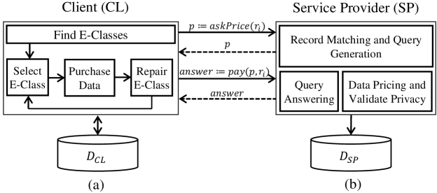
Figure 3: Framework overview.

4.2 Solution Overview

Figure 3 shows the PACAS system architecture consisting of two main units that execute functions for CL and SP. Figure 3(a) shows the CL unit containing four modules. The first module finds equivalence classes in $R_{\textit{CL}}$. An equivalence class (eq) is a set of cells in $R_{\textit{CL}}$ with equal values in order for $R_{\textit{CL}}$ to satisfy $\Sigma$ [2]. The next three modules apply an iterative repair for the eqs. These modules select an eq, purchase accurate value(s) of dirty cell(s) in the class, and then repair the cells using the purchased value. If the repairs contain generalized values, the CL unit must verify consistency of the generalized relation against the defined FDs. The cleaning iterations continue until $\mathcal{B}$ is exhausted or all the eqs are repaired. We preferentially allocated the budget $\mathcal{B}$ to cells in an eq based on the proportion of errors in which the cells (in an eq) participate. Figure 3(b) shows the SP unit. The Record Matching module receives a request $r_{i}=(t,A,l)$ from CL, identifies a matching tuple $t^{\prime}$ in $R_{\textit{SP}}$, and returns $t^{\prime}[A]$ at the level $l$ according to the VGH. The Data Pricing and Validate Privacy module computes prices for these requests, and checks whether answering these requests will violate (X,Y,L)-anonymity in $R_{\textit{SP}}$. If so, the request is not safe to be answered. The Query Answering module accepts payment for requests, and returns the corresponding answers to CL.

5 Limiting Disclosure of Sensitive Data

The SP must carefully control disclosure of its curated and sensitive data to the CL. In this section, we describe how the SP services an incoming client request for data, validates whether answering this request is safe (in terms of violating (X,Y,L)-anonymity), and the data pricing mechanism that facilitates this interaction.

5.1 Record Matching and Query Generation

Given an incoming CL request $r_{i}=(t,A,l)$, the SP must translate $r_{i}$ to a query that identifies a matching (clean) tuple $t^{\prime}$ in $R_{\textit{SP}}$, and returns $t^{\prime}[A]$ at level $l$. To answer each request, the SP charges the CL a price that is determined by the level $l$ of data disclosure and the adherence of $t^{\prime}[A]$ to the privacy model. To translate a request $r$ to a GQ $G_{r}$, we assume a schema mapping exists between $R_{\textit{SP}}$ and $R_{\textit{CL}}$, with similarity operators $\approx$ to compare the attribute values. This can be modeled via matching dependencies (MDs) in SP [5].

Example 5.1

Consider a request $r\!\!=\!\!(t_{2},{\sf MED},l^{\sf MED}_{1})$ that requests the medication of the patient in tuple $t_{2}$ at level $l^{\sf MED}_{1}$. To translate $r$ into a generalized query $G_{r}=\langle Q_{r},L_{r}\rangle$, we use the values of the QI attributes GEN and AGE in tuple $t_{2}$. We define a query $Q_{r}(R_{\textit{SP}})=\Pi_{\sf MED}(\sigma_{{\sf GEN}=t_{2}[{\sf GEN}]\wedge{\sf AGE}=t_{2}[{\sf AGE}]}$  $(R_{\textit{SP}}))$ requesting the medications of patients in $R_{\textit{SP}}$ with the same gender and age as the patient in tuple $t_{2}$. The GQ $G_{r}$ level is equal to the level of the request, i.e. $L_{r}=\{l^{\sf MED}_{1}\}$. The query $Q_{r}$ is generated from an assumed matching dependency (MD) $R_{\textit{CL}}[{\sf GEN}]=R_{\textit{SP}}[{\sf GEN}]\wedge R_{\textit{CL}}[{\sf AGE}]=R_{\textit{SP}}[{\sf AGE}]\rightarrow R_{\textit{CL}}[{\sf MED}]=R_{\textit{SP}}[{\sf MED}]$ that states if the gender and age of two records in SP and CL are equal, then the two records refer to patients with the same prescribed medication.

5.2 Enforcing Privacy

Recall from Section 2.4.1 that (X,Y,L)-anonymity extends (X,Y)-anonymity to consider the attribute domain semantics. Given a GQ, the SP must determine whether it is safe to answer this query, i.e., decide whether disclosing the value requested in $r_{i}$ violates (X,Y,L)-anonymity (defined in Defn. 4). In this section, we formalize the privacy guarantees of (X,Y,L)-anonymity, and in the next section, review the SafePrice data pricing algorithm that assigns prices to GQs to guarantee (X,Y,L)-anonymity.

(X,Y,L)-anonymity applies tighter privacy restrictions compared to (X,Y)-anonymity by tuning the parameter $L$ (determined by the data owner). At higher levels of $L$, it becomes increasingly more difficult to satisfy the (X,Y,L)-anonymity condition, while (X,Y,L)-anonymity reduces to (X,Y)-anonymity at $l_{i}=0$ for every $l_{i}\in L$. We formally state this in Theorem 5.1. (X,Y,L)-anonymity is a semantic extension of (X,Y)-anonymity. Similar extensions can be defined for PPDP models such as (X,Y)-privacy, $l$-diversity, $t$-closeness. Unfortunately, all these models do not consider the data semantics in the attribute DGHs and VGHs [11].

Theorem 5.1

Consider a relation $R$ and let $X$ and $Y$ be two subsets of attributes in $R$. Let $L_{1}$ and $L_{2}$ be levels of the attributes in $Y$ with $L_{1}\leq L_{2}$, i.e. every level of $L_{1}$ is lower than or equal to its corresponding level in $L_{2}$. The following holds for relation $R$ with a fixed $k>1$:

1. If $R$ is $(X,Y,L_{2})$-anonymous it is also $(X,Y,L_{1})$-anonymous, but not vice versa (i.e. $R$ can be $(X,Y,L_{1})$-anonymous but not $(X,Y,L_{2})$-anonymous).

2. For any levels $L$ of attributes in $Y$, if $R$ is (X,Y,L)-anonymous, it is also (X,Y)-anonymous.

Proof of Theorem 5.1. In the first item, if $R$ is $(X,Y,L_{2})$-anonymous, then for every $t$, $|G_{1}^{t}(R)|\geq k$ in which $G_{1}^{t}=\langle Q^{t},L_{1}\rangle$. Considering $G_{2}^{t}=\langle Q^{t},L_{2}\rangle$, we can claim $|G_{2}^{t}(R)|\geq k$, which proves $R$ is also $(X,Y,L_{1})$-anonymous. The claim holds because if $Q^{t}$ has $n$ answers in levels of $L_{1}$, it will have fewer or equal number of answers in the higher level $L_{2}$ since different values in levels of $L_{1}$ may be replaced with the same ancestors in the levels of $L_{2}$. The second item holds because if $R$ is (X,Y,L)-anonymous it is also $(X,Y,L^{\bot})$-anonymous where $L^{\bot}$ contains the bottom levels of attributes in $Y$; due to $L^{\bot}\leq L$ and item 1. If $R$ is $(X,Y,L^{\bot})$-anonymous, then every value of $X$ appears with $k$ ground values and we can conclude it is (X,Y)-anonymous. $\square$

5.3 Pricing Generalized Queries.

PPDP models have traditionally been used in non-interactive settings where a privacy-preserving table is published once. We take a user-centric approach and let users dictate the data they would like published. We apply PPDP in an interactive setting where values from relation $R_{\textit{SP}}$ are published incrementally according to (user) CL requests, while verifying that the disclosed data satisfies (X,Y,L)-anonymity [12]. We adopt a data pricing scheme that assigns prices to GQs by extending the baseline data pricing algorithm defined in [29] to guarantee (X,Y,L)-anonymity. We review this baseline pricing algorithm next.

Baseline Data Pricing.    The baseline pricing model computes a price for a query $Q$ over relation $R$ according to the amount of information revealed about $R$ when answering $Q$ [29].

Given a query $Q$ over a relation $R$ (a database with single relation $R$), the baseline pricing model determines the price of $Q$ based on the amount of information revealed about $R$ by answering $Q$. Let $\mathcal{I}$ be a set of possible relations that the buyer believes to be $R$, representing his initial knowledge of $R$. As the buyer receives answers to $Q(R)$, he gains new knowledge, allowing him to eliminate relations $R^{\prime}$ from $\mathcal{I}$, which provide a different answer $Q(R^{\prime})\neq Q(R)$. This set of eliminated instances $R^{\prime}$ is called the conflict set of $Q$ denoted as $\mathcal{C}_{Q}$, and intuitively represents the amount of information that is revealed by answering $Q$ (Figure 4). As more queries are answered, the size of $\mathcal{I}$ is reduced. We can apply a set function that uses $\mathcal{C}_{Q}$ to compute a price for $Q$. We can use the weighted cover set function with predefined weights assigned to the relations in $\mathcal{I}$. Query prices are computed by summing the weights for relations in $\mathcal{C}_{Q}$, which has been shown to give arbitrage-free prices [29]. In practice, the set $\mathcal{I}$ is usually infinite making it infeasible to implement. To circumvent this problem, a smaller, finite subset $\mathcal{S}$ called the support set is used to generate arbitrage-free prices [29]. The support set is defined as the neighbors of $R$, generated from $R$ via tuple updates, insertions, and deletions. The values that are used to generate the support set are from the same domain of the original relation $R$.

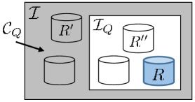
Figure 4: Possible relations $\mathcal{I}$, conflict set $\mathcal{C}_{Q}$ and admissible relations $\mathcal{I}_{Q}$ for query $Q$.

Input : A query $Q$, a database $D$, support set $\mathcal{S}$, weight function $w$

Output : Price to answer $Q$

1

2$p\leftarrow 0$;

3for $D^{\prime}\in\mathcal{S}$ do

4       if $Q(D^{\prime})\neq Q(D)$ then  $p\leftarrow p+w(D^{\prime})$ ;

5      

return $p$;

Algorithm 1 $\textit{price}(Q,D,\mathcal{S},w)$ [29]

Several optimizations are applied to the baseline pricing, and its effectiveness is experimentally justified [29]. Most importantly, the relations in the support set can be modeled by update operations. That is, we generate each relation in $\mathcal{S}$ from $R$ by applying its corresponding update operation and use the resulting relation to compute the value of the weighted function as the final price. We roll-back the update to restore $R$, and continue this process to compute the weighted function using other relations in $\mathcal{S}$. We avoid storing all databases in $\mathcal{S}$ to enable more efficient price computations.

Algorithm 1 provides pseudocode of the baseline algorithm. The algorithm takes query $Q$, database $D$, a support set $\mathcal{S}$, and a weight function $w$, and computes the price to answer $Q$ over $R$. The baseline algorithm is history-aware as input $\mathcal{S}$ excludes databases that were already considered by past queries.

SafePrice Algorithm.    We describe the SafePrice algorithm (originally introduced in [12]) that enforces (X,Y,L)-anonymity over $R$ (equivalently $R_{\textit{SP}}$ in our framework). We first present the definition of a safe query, i.e., criteria for a GQ to preserve (X,Y,L)-anonymity.

Definition 7

(Safe Query) Consider a GQ $G$ over a relation $R$ with schema $\mathcal{R}$, $X,Y\subseteq\mathcal{R}$, and levels $L$ corresponding to attributes in $Y$. Let $\mathcal{I}_{G}\subseteq\mathcal{I}$ be the set of relations $R^{\prime\prime}$ such that $G(R)=G(R^{\prime\prime})$. $G$ is safe (or preserves (X,Y,L)-anonymity of $R$) with value $k$, if for every tuple $t\in R$, there are at least $k$ tuples in the set of answers $\{t^{\prime\prime}\;|\;\exists R^{\prime\prime}\in\mathcal{I}_{G},t^{\prime\prime}\in{G}^{t}(R^{\prime\prime})\}$ where ${G}^{t}=\langle{Q}^{t},L\rangle$ is a GQ with ${Q}^{t}(R^{\prime\prime})=\Pi_{Y}(\sigma_{X=t[X]}(R^{\prime\prime}))$.

In Definition 7, $\mathcal{I}_{G}$ represents the set of relations that the buyer believes $R$ is drawn from after observing the answer $G(R)$. If there are at least $k$ tuples in the answer set of ${G}^{t}$ over $\mathcal{I}_{G}$, this indicates that the buyer does not have enough information to associate the values in $X$ to less than $k$ values of $Y$ at level $L$, thus preserving (X,Y,L)-anonymity. If the SP determines that a GQ is safe, he will assign a finite price relative to the amount of disclosed information about $R$.

Algorithm 2 presents the SafePrice details. The given support set $\mathcal{S}$ represents the user’s knowledge about relation $R$ after receiving the answer to past purchased queries. We maintain a set $\mathcal{S}_{G}$ that represents all admissible relations after answering $G$ and captures the user’s posterior knowledge about $R$ after answering $G$. We use $\mathcal{S}_{G}$ to check whether answering $G$ is safe. This is done by checking over instances in $\mathcal{S}_{G}$ whether values in $X$ are associated with at least $k$ values of $Y$ using the query ${G}^{t}$. The price for a query is computed by summing the weights of the inadmissible relations in the conflict set $\mathcal{C}_{G}=\mathcal{S}\setminus\mathcal{S}_{G}$ (Line 2). Similar to the baseline pricing, we use the support set $\mathcal{S}$ and admissible relations $\mathcal{S}_{G}$ rather than $\mathcal{I}$ and $\mathcal{I}_{G}$, respectively. We iterate over tuples $t\in R$ (Line 2), and check whether values in $X$ are associated with less than $k$ values in $Y$ over relations in $\mathcal{S}_{G}$. If so, we return an infinite price reflecting that query $G$ is not safe (Line 2).

Proposition 1

If the input GQ is not safe, Algorithm 2 preserves (X,Y,L)-anonymity by returning an infinite price.

Proof sketch: According to Definition 7, if $G$ violates (X,Y,L)-anonymity then for $t\in R$, there are less than $k$ answers to ${G}^{t}$ over relations in $\mathcal{I}_{G}$. Since $\mathcal{S}_{G}\subseteq\mathcal{I}_{G}$, there will be less than $k$ answers to ${G}^{t}$ over relations in $\mathcal{S}_{G}$, meaning Algorithm 2 assigns infinite price to $G$ in Line 2. Note that if Algorithm 2 returns an infinite price, it does not imply $G$ is unsafe (this only occurs when $\mathcal{S}=\mathcal{I}$).  

Input : $G$, $R$, $\mathcal{S}$, $w$

Output : Price of $G$

1

2$p\leftarrow 0$; $\mathcal{S}_{G}\leftarrow 0$;

3for $T\in\mathcal{S}$ do

4       if $G(T)=G(R)$ then  $\mathcal{S}_{G}\leftarrow\mathcal{S}_{G}\cup\{T\}$ ;

5       else  $p\leftarrow p+w(T)$ ;

6      

7for $t\in R$  do

8       $A\leftarrow\emptyset$;

9      for $R^{\prime\prime}\in\mathcal{S}_{G}$ do  $A\leftarrow A\cup{G}^{t}(R^{\prime\prime})$ ;

10      

11      if $|A|<k$ then return $\infty$;

12      

return $p$;

Algorithm 2 $\textit{SafePrice}(G,R,\mathcal{S},w)$

Given the interactive setting between the CL and the SP, we must ensure that all (consecutively) disclosed values guarantee (X,Y,L)-anonymity over $R$. We ensure that SafePrice is history-aware by updating the support set $\mathcal{S}$ after answering each GQ. The SP uses the pricing function in Algorithm 2 to update $\mathcal{S}$ to reflect the current relations $R^{\prime}$ that have been eliminated by answering the latest GQ. The SP implements $\textit{AskPrice}(r_{i},R_{\textit{SP}})$ (cf. Figure 3) by translating $r_{i}$ to a GQ, and then invoking SafePrice.

We assume that requesting a query price is free. We acknowledge that returning prices might leak information about the data being priced and purchased. This problem is discussed in the data pricing literature, particularly to incentivize data owners to return trustful prices when prices reveal information about the data (cf. [30] for a survey on this issue). We consider this problem as a direction of future work.

5.4 Query Answering

A CL data request is executed via the $\textit{Pay}(p,r_{i},R_{\textit{SP}})$ method, where she purchases the value in $r_{i}$ at price $p$. The Query Answering module executes $\textit{Pay}(p,r_{i},R_{\textit{SP}})$ via SP accepts payment, translates $r_{i}$ to a GQ, and returns the answer over $R_{\textit{SP}}$ to CL. Lastly, SP updates the support set $\mathcal{S}$ to ensure SafePrice has an accurate history of disclosed data values.

We note that all communication between CL and SP is done via the AskPrice and Pay methods (provided by SP). We assume there is a secure communication protocol between the CL and SP, and that all data transfer is protected and encrypted. The model is limited to a single SP that sells data at non-negotiable prices. We intend to explore general cases involving multiple SP providers and price negotiation as future work.

6 Data Cleaning with Generalized Values

Existing constraint-based data repair algorithms that propose updates to the data to satisfy a set of data dependencies assume an open-access data model with no data privacy restrictions [2, 31, 32, 33, 34]. In these repair models, inadvertent data disclosure can occur as the space of repair candidates is not filtered nor transformed to obscure sensitive values. A privacy-aware data repair algorithm must address the challenge of providing an accurate repair to an error while respecting data generalizations and perturbations to conceal sensitive values.

In earlier work, we introduced SafeClean, a data repair algorithm that resolves errors in a relation $R_{\textit{CL}}$ using data purchased from a service provider $R_{\textit{SP}}$ [12]. The key distinctions of SafeClean from past work include: (i) SafeClean interacts with the service provider, SP, to purchase trusted values under a constrained budget $\mathcal{B}$. This eliminates the overhead of traversing a large search space of repair candidates; and (ii) SafeClean tries to obtain values with highest utility from SP for repairing CL. However, the existing SafeClean algorithm grounds all purchased values thereby not allowing generalized values in $R_{\textit{CL}}$. In this paper, we extend SafeClean to consider generalized values in $R_{\textit{CL}}$ by re-defining the notion of consistency between a relation and a set of FDs (Section 3.2), and revising the budget allocation algorithm to requests according to the number of errors in which cells in an equivalence participate (Section 6.4). In contrast, the existing SafeClean provides fixed budget allocations. We give an overview of our cleaning algorithm and subsequently describe each component in detail.

6.1 Overview

For a fixed number of FDs $\Sigma$, the problem of finding minimal-cost data repairs to $R_{\textit{CL}}$ such that $R_{\textit{CL}}$ satisfies $\Sigma$ is NP-complete [2]. Due to these intractability results, we necessarily take a greedy approach that cleans cell values in $R_{\textit{CL}}$ that maximally reduce the overall number of errors w.r.t. $\Sigma$. This is in similar spirit to existing techniques that have used various weighted cost functions [2, 35] or conflict hypergraphs [33] to model error interactions among data dependencies in $\Sigma$.

Given $R_{\textit{CL}}$ and $\Sigma$, we identify a set of error cells that belong to tuples that falsify some $\sigma\in\Sigma$. For an error cell $e\in\mathcal{E}$, we define eq($e$) as the equivalence class to which $e$ belongs. An equivalence class is a set of database cells with the same value such that $\Sigma$ is satisfied [2]. We use eqs for two reasons: (i) by clustering cells into eqs, we determine a repair value for a group of cells rather than an individual cell, thereby improving performance; and (ii) we utilize every cell value within an eq to find the best repair.

The SafeClean algorithm repairs FD errors by first finding all the eqs in $R_{\textit{CL}}$. The algorithm then iteratively selects an eq, and purchases the true value of a cell, and updates all dirty cells in the same class to the purchased value. The SP may decide that returning a generalized value is preferred to protect user sensitive data in $R_{\textit{SP}}$. If so, then the CL must validate consistency of its data including these generalized values. At each iteration, we repair the eq class with cells that participate in the largest number of FD errors. At each iteration, SafeClean assigns a portion of the budget $\mathcal{B}$ that is proportional to the number of errors relative to the total number of errors in $R_{\textit{CL}}$ (this new extension to SafeClean is discussed in Section 6.4). SafeClean continues until all the eqs are repaired, or the budget is exhausted.

Input : $R_{\textit{CL}}$, $R_{\textit{SP}}$, $\Sigma$, $\mathcal{B}$

Output : Clean $R_{\textit{CL}}^{\prime}$

1 $R_{\textit{CL}}^{\prime}\leftarrow R_{\textit{CL}}$;

2 $\textit{EQ}\leftarrow\textit{GenerateEQs}(R_{\textit{CL}}^{\prime},\Sigma)$;

3 $B\leftarrow\mathcal{B}$;

4 for $\textit{eq}\in\textit{EQ}$ do

5      if $\textit{Resolved}(\textit{eq})$ then $\textit{EQ}\leftarrow\textit{EQ}\setminus\{\textit{eq}\}$;

6      

7while $B>0$ and $\textit{EQ}\neq\emptyset$ do

8       $\textit{eq}\leftarrow\textit{Select}(\textit{EQ});$

9       $r_{i}\leftarrow\textit{GenerateRequest}(\textit{eq},\alpha_{i}\times B,R_{\textit{SP}});$

10       if $r_{i}\neq{\sl null}$ then

11             $p_{i}\leftarrow\textit{AskPrice}(r_{i},R_{\textit{SP}});$

12             $u_{i}\leftarrow\textit{Pay}(p_{i},r_{i},R_{\textit{SP}})$;

13             $B\leftarrow B-p_{i}$;

14             $\textit{ApplyRepair}(\textit{eq},u_{i})$;

15      $\textit{EQ}\leftarrow\textit{EQ}\setminus\textit{eq}$;

return $R_{\textit{CL}}^{\prime}$

Algorithm 3 $\textit{SafeClean}(R_{\textit{CL}},R_{\textit{SP}},\Sigma,\mathcal{B})$

SafeClean Algorithm. Algorithm 3 gives details of SafeClean’s overall execution. The algorithm first generates the set of eqs via GenerateEQs in Line 3. Equivalence classes containing only one value are removed since there is no need for repair. In Line 3, SafeClean selects an equivalence class $\textit{eq}_{i}$ with cells participating in the largest number of violations for repair (further details in Section 6.3). To repair the error cells in $\textit{eq}_{i}$, SafeClean generates a request $r_{i}$ using GenerateRequest that requests a repair value for a cell in $\textit{eq}_{i}$ (Line 3). This request is made at the lowest possible level (less than $l_{max}$) at a price allowable within the given budget. The algorithm assigns a fraction of the remaining budget, i.e. $\alpha_{i}\times B$ ($B\leq\mathcal{B}$ is the remaining budget) to purchase data at each iteration. This fraction depends on the number of violations in $\textit{eq}_{i}$ (cf. Section 6.4 for details). If such a request can be satisfied, the value(s) are purchased and applied (Lines 3-3). If there is insufficient budget remaining to purchase a repair value, then the eq cannot be repaired. In either case, SafeClean removes $\textit{eq}_{i}$ from EQ and continues with the next eq (Line 3). SafeClean terminates when $\mathcal{B}$ is exhausted, or there are no eqs are remaining. We present details of eq generation, selection, request generation, and data purchase/repair in the following sections.

6.2 Generating Equivalence Classes

The eqs are generated by GenerateEQs in Algorithm 4 that takes as input $R_{\textit{CL}}$ and $\Sigma$, and returns the set of eqs EQ. For every cell $c_{i}\in R_{\textit{CL}}$, the procedure initializes the eq of $c_{i}$ as $\textit{eq}(c_{i})=\{c_{i}\}$, and adds it to the set of eqs EQ (Line 4). We then iteratively merge the eqs of any pair of cells $c_{1}=t_{1}[B],c_{2}=t_{2}[B]$ if there is a FD $\varphi:A\rightarrow B\in\Sigma$, $t_{1}[A]=t_{2}[A]$, and both $t_{1}[A]$ and $t_{2}[A]$ are ground. The procedure stops and returns EQ when no further pair of eqs can be merged.

Input : $R_{\textit{CL}}$, $\Sigma$,

Output : The set of equivalence classes EQ

1

2$\textit{EQ}\leftarrow\emptyset$;

3for $c_{i}\in R_{\textit{CL}}$ do  $\textit{EQ}\leftarrow\textit{EQ}\cup\{\{c_{i}\}\}$ ;

4

5for every $t_{1},t_{2}\in R_{\textit{CL}}$ and $\varphi:A\rightarrow B\in\Sigma$ do

6       if $t_{1}[A]=t_{2}[A]$  then  $\textit{merge}(\textit{EQ}(t_{1}[B]),\textit{EQ}(t_{2}[B]))$ ;

7      

8return EQ;

Algorithm 4 $\textit{GenerateEQs}(R_{\textit{CL}},\Sigma)$

Example 6.1

Given FD $\varphi:[{\sf GEN},{\sf DIAG}]\rightarrow[{\sf MED}]$ in Table 3, since $t_{1}$, $t_{2}$ and $t_{3}$ have the same attribute values on GEN and DIAG, we merge $t_{1}[{\sf MED}]$, $t_{2}[{\sf MED}]$ and $t_{3}[{\sf MED}]$ into the same $\textit{EQ}_{1}$. Similarly, we cluster $t_{4}$ and $t_{5}$ into the same $\textit{EQ}_{2}$.

6.3 Selecting Equivalence Classes for Repair

In each iteration of Algorithm 3, we repair the cells in an eq $\textit{eq}_{i}$ that will resolve the most errors in $R_{\textit{CL}}$ w.r.t. $\Sigma$. To achieve this goal, we choose $\textit{eq}_{i}$ as the eq with cells participating in the largest number of errors. For a cell $c_{j}\in R_{\textit{CL}}$ and an FD $\varphi:A\rightarrow B\in\Sigma$, let $\mathcal{E}(R_{\textit{CL}},\varphi,c_{j})$ be the set of errors $\{{t_{1}},{t_{2}}\}$ w.r.t. $\varphi$ and $c_{j}\in\{t_{1}[A],t_{1}[B],t_{2}[A],t_{2}[B]\}$. For an eq $\textit{eq}_{i}$, let $\mathcal{E}(R_{\textit{CL}},\varphi,\textit{eq}_{i})=\bigcup_{c_{j}\in\textit{eq}_{i}}\mathcal{E}(R_{\textit{CL}},\varphi,c_{j})$ and $\mathcal{E}(R_{\textit{CL}},\Sigma,\textit{eq}_{i})=\bigcup_{\varphi\in\Sigma}\mathcal{E}(R_{\textit{CL}},\varphi,\textit{eq}_{i})$. The eq $\textit{eq}_{i}$ returned by Select in Line 3 of Algorithm 3 is the eq with the largest number of errors in $\mathcal{E}(R_{\textit{CL}},\Sigma,\textit{eq}_{i})$. In other words, this is the number of tuple pairs that every cell in $\textit{eq}_{i}$ participates, summed over all FDs in $\Sigma$.

Example 6.2

We continue Example 6.1 with $\textit{EQ}_{1}$ and $\textit{EQ}_{2}$. According to our error definition, given FD $\varphi:[{\sf GEN},{\sf DIAG}]\rightarrow[{\sf MED}]$, $\textit{EQ}_{1}$ is involved in three errors with tuples ($\{t_{1},t_{2}\}$, $\{t_{1},t_{3}\}$ and $\{t_{2},t_{3}\}$), while $\textit{EQ}_{2}$ has one error ($\{t_{3},t_{4}\}$). Hence, our algorithm will select $\textit{EQ}_{1}$ to repair first.

6.4 Data Request Generation

To repair cells in $\textit{eq}_{i}$, we generate a request $r_{i}=\langle c,l\rangle$ by GenerateRequest (Algorithm 5) that requests accurate and trusted value of a cell $c\in\textit{eq}_{i}$ at level $l$ from $R_{\textit{SP}}$. There are two restrictions on this request: (i) the price must be within the budget $\alpha_{i}\times\mathcal{B}$, and (ii) the level $l$ must be $\leq l_{\textit{max}}$. The value $\alpha_{i}$ is defined as follows:

$$\alpha_{i}=\frac{\mathcal{E}(R_{\textit{CL}},\Sigma,\textit{eq}_{i})}{\sum_{\textit{eq}_{j}\in\textit{EQ}}{\mathcal{E}(R_{\textit{CL}},\Sigma,\textit{eq}_{j})}}.$$

In this definition, the allocated budget $\alpha_{i}\times B$ to each iteration is proportional to the number of FD violations in $\textit{eq}_{i}$, and also depends on the total number of errors in $R_{\textit{CL}}$. This allocation model improves upon previous work that decreases the budget allocated to the $i^{th}$-request by a factor of $\frac{1}{i}$, and does not adjust the allocation to the number of errors in which a cell participates [12]. Note that if the price paid for $r_{i}$ (i.e. $p_{i}$) is less than this allocated budget, the remaining budget carries to the next iteration through $B$.

If there is no such request, GenerateRequest returns null, indicating that $\textit{eq}_{i}$ cannot be repaired with the allocated budget (Line 5). If there are several requests that satisfy (i) and (ii), we follow a greedy approach and select the request at the lowest level with the price to break ties (Line 5). For a cell $c_{i}\in\textit{eq}_{i}$, LowestAffordableLevel in Line 5 finds the lowest level in which the value of $c_{i}$ can be purchased from $R_{\textit{SP}}$ considering the restrictions in (i) and (ii). Our greedy algorithm spends most of the allocated budget $\alpha_{i}\times B$ in the current iteration. An alternative approach is to select requests with the highest acceptable level ($l_{\textit{max}}$) to preserve the budget for future iterations.

Input : eq $C$, budget $b$ and $R_{\textit{SP}}$.

Output : Request $r_{i}$

1

2$l\leftarrow l_{h}$; $p\leftarrow\infty$; $c\leftarrow{\sl null}$;

3for $c_{i}\in C$ do

4       $l_{i}\leftarrow\textit{LowestAffordableLevel}(c_{i},b,l_{\textit{max}},R_{\textit{SP}})$;

5       $p_{i}\leftarrow\textit{AskPrice}(\langle c_{i},l_{i}\rangle,R_{\textit{SP}})$;

6       if $l_{i}<l$ or $(l_{i}==l$ and $p_{i}\leq p)$ then

7            $c\leftarrow c_{i}$;$\;\;l\leftarrow l_{i}$;$\;\;p\leftarrow p_{i}$;

8if $c\neq{\sl null}$ then return $\langle c,l\rangle$;

9return null;

Algorithm 5 $\textit{GenerateRequest}(C,b,R_{\textit{SP}})$

6.5 Purchase Data and Repair

To repair the cells in $\textit{eq}_{i}$, Algorithm 3 invokes $\textit{Pay}(r_{i},R_{\textit{SP}})$ to purchase the trusted value $u_{i}$ and replaces the value of every cell in $\textit{eq}_{i}$ with $u_{i}$ in ApplyRepair. The algorithm then removes the eq $\textit{eq}_{i}$ from EQ and continues to repair the next eq. The algorithm stops when there is no eq to repair or the budget is exhausted.

Example 6.3

Continuing from Example 6.2, since $\textit{EQ}_{1}$ has the largest number of errors, we purchase the trusted value from $R_{\textit{SP}}$ to repair $\textit{EQ}_{1}$ first. If the purchased value is general value NSAID, we update all cells in $\textit{EQ}_{1}$, i.e., $t_{1}[{\sf MED}]$, $t_{2}[{\sf MED}]$ and $t_{3}[{\sf MED}]$ to NSAID to resolve the inconsistency.

6.6 Complexity Analysis

We analyze the complexity of SafeClean’s modules:

• Identifying errors involves computing equivalence classes, and selecting an equivalence class for repair. In the worst case, this is quadratic in the number of tuples in $R_{\textit{CL}}$.

• For each data request to resolve an error, executing SafePrice and $pay$ rely on $R_{\textit{SP}}$, the support set $\mathcal{S}$, and the complexity of GQ answering. We assume the size of $\mathcal{S}$ is linear w.r.t the size of $R_{\textit{SP}}$. The complexity of running GQs is the same as running SQL queries. Thus, all procedures run in polynomial time to the size of $R_{\textit{SP}}$.

• In applyRepair, for each returned value from SP, we update the error cells in $R_{\textit{CL}}$ for each equivalence class and each FD, taking time on the order of $\mathcal{O}(|\mathcal{E}||A||\Sigma|)$ for attribute domain size $|A|$. We must update the affected cells in the equivalence class, and their dirty scores; both taking time bounded by the number of cells in $R_{\textit{CL}}$. Hence, Algorithm 3 runs in polynomial time to the size of $R_{\textit{SP}}$ and $R_{\textit{CL}}$.

7 Experiments

Our evaluation focuses on the following objectives:

1. We evaluate the impact of generalized values on the repair error, and the runtime performance. In addition, we study the proportion of generalized repair values that are recommended for varying budget levels.

2. The efficiency and effectiveness of SafePrice to generate reasonable prices that allow SafeClean to effectively repair the data.

3. We evaluate the repair error and scalability of SafeClean as we vary the parameters $k,l,e$ and $\mathcal{B}$ to study the repair error to runtime tradeoff.

4. We compare SafeClean against PrivateClean, a framework that explores the link between differential privacy and data cleaning [8]. We study the repair error to runtime tradeoff between these two techniques, and show that data randomization in PrivateClean significantly hinders error detection and data repair, leading to increased repair errors.

7.1 Experimental Setup

We implement PACAS using Python 3.6 on a server with 32 Core Intel Xeon 2.2 GHz processor with 64GB RAM. We describe the datasets, baseline comparative algorithm, metrics and parameters. The datasets, their schema, and source code implementation can be found at [36].

Table 5: Data characteristics.

	Clinical	Census	Food
$|R_{\textit{CL}}|$	345,000	300,000	30,000
$n$	29	40	11
$|\Pi_{A}(R)|$	61/73	17/250	248/70
$|{\sf VGH}^{A}|$	5/5	5/6	5/5

Table 6: Parameter values (defaults in bold).

Sym.	Description	Values
$\mathcal{B}$	budget	0.2, 0.4, 0.6, 0.8
$|\mathcal{S}|$	support set size	6, 8, 10, 12, 14
$l$	generalization level	0, 1, 2, 3, 4
$k$	#tuples in X-group	1, 2, 3, 4, 5
$e$	error rate	0.05, 0.1, 0.15, 0.2, 0.25

Datasets. We use three real datasets. Table 6 gives the data characteristics, showing a range of data sizes in the number of tuples ($|R_{\textit{CL}}|$), number of attributes ($n$), number of unique values in the sensitive attribute $A$ ($|\Pi_{A}(R)|$), and the height of the attribute ${\sf VGH}^{A}$ ($|{\sf VGH}^{A}|$). We denote sensitive attributes with an asterisk (*).

Clinical Trials (Clinical). The Linked Clinical Trials database describes patient demographics, diagnosis, prescribed drugs, symptoms, and treatment [37]. We select the country, gender, source and age as QI attributes. We define two FDs: (i) $\varphi_{1}:$ [age, overall_status, gender] $\to$ [drug_name*]; and (ii) $\varphi_{2}:$ [overall_status, timeframe, measure] $\to$ [condition*]. We construct attribute value generalization hierarchies (VGH) with five levels on attributes drug name and condition, respectively using external ontologies (Bioprotal Medical Ontology [38], the University of Maryland Disease Ontology [39], and the Libraries of Ontologies from the University of Michigan [40]). The average number of children per node in the VGH is eight.

Census. The U.S. Census Bureau provides population characteristics such as education level, years of schooling, occupation, income, and age [41]. We select sex, age, race, and native country as QI attributes. We define two FDs: (i) $\varphi_{3}:$ [age, education-num] $\to$ [education*]; and (ii) $\varphi_{4}:$ [age, industry code, occupation] $\to$ [wage-per-hour*]. We construct VGH on attributes wage-per-hour and education by stratifying wage and education levels according to hierarchies from US statistics [42], and the US Department of Education [43]. The average number of children per node is five.

Food Inspection (Food). This dataset contains violation citations of inspected restaurants in New York City describing the address, borough, zipcode, violation code, violation description, inspection type, score, grade. We define inspection type, borough, grade as QI attributes. We define two FDs: (i) $\sigma_{5}:$ [borough, zipcode] $\to$ [address*]; and (ii) $\sigma_{6}:$ [violation code, inspection type] $\to$ [violation description*]. We construct attribute VGH on address and violation description by classifying streets into neighborhoods, districts, etc, and extracting topic keywords from the description and classifying the violation according to the Food Service Establishment Inspection Code [44]. The average number of children per node in the VGH is four.

For each dataset, we manually curate a clean instance $R_{\textit{SP}}$ according to the defined FDs, verify with external sources and ontologies, and is used as the ground truth. To create a dirty instance $R_{\textit{CL}}$, we duplicate $R_{\textit{SP}}$ to obtain $R_{\textit{CL}}$, and use BART, an error generation benchmarking tool for data cleaning applications to inject controlled errors in the FD attributes [45]. We use BART to generate constraint-induced errors and random errors, and define error percentages ranging from 5% to 25%, with respect to the number of tuples in a table. We use BART’s default settings for all other parameters.

Comparative Baseline. The closest comparative baseline is PrivateClean, a framework that explores the link between differential privacy and data cleaning [8]. PrivateClean provides a mechanism to generate $\epsilon$-differentially private datasets on numerical and discrete values from which a data analyst can apply data cleaning operations. PrivateClean proposes randomization techniques for discrete and numeric values, called Generalized Randomized Response (GRR), and applies this across all attributes. To guarantee a privatized dataset with discrete attributes is $\epsilon$-differentially private at confidence $(1-\alpha)$, a sufficient number of distinct records is needed. In our comparison evaluation, we set $\alpha=0.05$, and the degree of privacy $p=0.5$ (applied uniformly across the attributes and equivalent to $\epsilon$ for discrete attributes [8]). Since PrivateClean does not directly propose a data cleaning algorithm, but rather data cleaning operators, we apply the well-known Greedy-Repair [2] FD repair algorithm to generate a series of updates to correct the FD violations. We use the transform() operation to represent each of these updates in PrivateClean, and use the source code provided by the authors in our implementation. We choose the Greedy-Repair algorithm for its similarity to our repair approach; namely, to repair cells on an equivalence class basis, and to minimize a cost function that considers the number of data updates and the distance between the source and target values.

Metrics. We compute the average runtime over four executions. To measure the quality of the recommended repairs, we define the repair error of a cell as the distance between a cell’s true value and its repair value. We use the semantic distance measure, $\delta(v,v^{\prime})$, in Section 3.1, that quantifies the distance between two values $v$ (suppose a true value), and $v^{\prime}$ (a repair value) in the attribute value generalization hierarchy, and considers the distribution of $v$ and $v^{\prime}$ in the relation. We assume a cell’s value, and its repair are both in the generalization hierarchy. The repair error of a relational instance is computed as the sum of the repair errors across all cells in the relation. We use the absolute value of the repair error in our experiments (denoted as $\delta$). Similar to other error metrics (such as mean squared error), lower error values are preferred.

Parameters. Unless otherwise stated, Table 6 shows the range of parameter values we use, with default values in bold. We vary the following parameters to evaluate algorithm performance: (i) the budget $\mathcal{B}$; (ii) the size of the support set $|\mathcal{S}|$ in the pricing function; (iii) $l$ (the lower bound of generalization); (i) $k$, the number of tuples in an $X$-group; and (vi) the error rate $e$ in $R_{\textit{CL}}$.

7.2 Generalized Values

We measure the proportion of generalized values that are returned for varying levels of the budget $\mathcal{B}$. Since a repair value may be returned at any level of the VGH, we compute the semantic distance between the generalized value $v$ and the corresponding ground value $v^{\prime}$ in the CL. We normalize the distance between ($v,v^{\prime}$) into four ranges: [0-0.25], [0.25-0.5], [0.5-0.75], [0.75-1], where a distance of zero indicates $v$ and $v^{\prime}$ are both ground values.

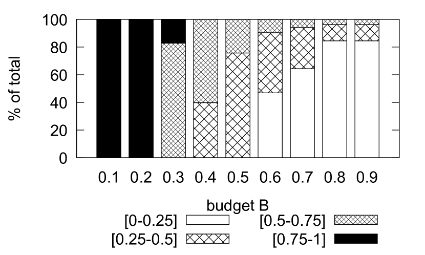
Figure 5: Ratio of gen. values.

Figure 6: Error vs. gen. values.

Figure 7: Runtime vs. gen. values.

Figure 5 shows the relative proportions for varying $\mathcal{B}$ values over the clinical dataset. As expected, the results show that the proportion of generalized values at the highest levels of the VGH occur for low $\mathcal{B}$ values since we can only afford (cheaper) generalized values under a constrained budget. In contrast, for $\mathcal{B}$ values close to 0.9, close to $85\%$ of the repair values are specific, ground values with a distance range of [0, 0.25], while the remaining $15\%$ are generalized values at the next level. We observe that for $\mathcal{B}>0.6$ approximately 70% of the total repair values are very close to the ground value (where distance is at [0-0.25]), indicating higher quality repairs.

We evaluate the impact on the runtime to repair error tradeoff when an increasing number of generalized values occur in the repaired relation. We control the number of generalized values indirectly via the number of error cells under a constrained budget $\mathcal{B}=0.1$ where it is expected that close to all repair recommendations will be general values. Figure 6 and Figure 7 show the repair error and runtime curves over the clinical data, respectively. As expected, we observe for an increasing number of generalized values, the repair error increases as the constrained budget leads to more values returned at the highest * generalized value, thereby increasing the distance between ground-truth relation and repaired relation. In contrast, the increased number of generalized values leads to lower runtimes due to the increased number of unsatisfied query requests.

7.3 SafePrice Efficiency and Effectiveness

Figure 8: Repair error vs. $|\mathcal{S}|$.

The SafePrice algorithm relies on a support set $\mathcal{S}$ to determine query prices by summing the weights of discarded instances from the conflict set $\mathcal{C}$. These discarded instances represent the knowledge gained by CL. We vary the size of the initial $\mathcal{S}$ to determine its influence on the repair error ($\delta$), and the overall runtime. Figure 8 shows a steady decrease in the repair error for increasing $|\mathcal{S}|$. As $|\mathcal{S}|$ grows, the SP is less restrictive to answer GQs and fewer requests are declined at lower levels. As more requests are answered at these lower levels, the repair error decreases. Figure 9 shows that the SafePrice runtime scales linearly with increasing $|\mathcal{S}|$, making it feasible to implement in practice. From Figures 8 and 9, we determine that SafePrice achieves an average 6% reduction in the repair error at a cost of 16m runtime. This is expected due to the additional time needed to evaluate the larger space of instances to answer GQs. Comparing across the three datasets, the data sizes affect runtimes as a larger number of records must be evaluated during query pricing. This is reflected in longer runtimes for the larger clinical and census datasets.

7.4 SafePrice Parameter Sensitivity

Figure 9: Runtime vs. $|\mathcal{S}|$.

Figure 10: Repair error vs. $k$.

Figure 11: Runtime vs. $k$.

Figure 12: Repair error vs. $l$.

Figure 13: Runtime vs. $l$.

Figure 14: Repair error vs. $e$.

Figure 15: Runtime vs. $e$.

Figure 16: Repair error vs. $\mathcal{B}$.

Figure 17: Runtime vs. $\mathcal{B}$.

We vary the parameters $k$, GQ level $l$, error rate $e$, budget $\mathcal{B}$, and measure their influence on SafeClean repair error and runtime over all three datasets. We expect that enforcing more stringent privacy requirements through larger $k$ and $l$ values will result in larger repair errors. Figures 10 to 13 do indeed reflect this intuition.

In Figure 10, SafeClean experiences larger repair errors for increasing $k$ as generalizations to conceal sensitive values become increasingly dependent on the attribute domain and its VGH i.e., (X,Y,L)-anonymity indicates there must be at least $k$ values at a given level $l$ in the VGH. Otherwise, the data request is denied. Figure 11 shows that for increasing $k$, runtimes decrease linearly as query requests to satisfy more stringent $k$ become more difficult. On average, we observe that an approximate 10% improvement in runtime leads to a 7% increase in the repair error for each increment of $k$. Figures 12 and 13 show the repair error and runtime, respectively, as we vary the query level parameter $l$. The repair error increases, particularly after $l=3$ as more stringent privacy requirements are enforced, i.e., $l$ distinct values are required at each generalization level. This makes satisfying query requests more difficult, leading to unrepaired values and lower runtimes, as shown in Figure 13.

Figure 14 shows the repair error $\delta$ increases as we scale the error rate $e$. For a fixed budget, increasing the number of FD errors leads to a decreasing budget for each FD error. This makes some repairs unaffordable for the CL, leading to unrepaired values and an increased number of generalized repair values. This situation can be mitigated if we increase the budget $\mathcal{B}$. As expected, Figure 15 shows that the SafeClean runtime increases for an increasing number of FD violations, due to the larger overhead to compute more equivalance classes, compute prices to answer queries, and to check consistency in the CL.

Figures 16 and 17 show the repair error and runtime, respectively, as we vary the budget $\mathcal{B}$. For increasing budget allocations, we expect the SP to recommend more ground (repair) values, and lower repair error values, as shown in Figure 16. Given the larger budget allocations, the SP is able to answer a larger number of query requests, and must compute their query prices, thereby increasing algorithm runtime. We observe that an average 14% reduction in the repair error leads to an approximate 7% increase in runtime.

7.5 Comparative Evaluation

We compare SafeClean to PrivateClean, a framework for data cleaning on locally differentially private relations [8]. Section 7.1 describes the baseline algorithm parameter settings and configuration. Despite the differing privacy models, our evaluation aims to explore the influence of increasing error rates on the repair error $\delta$, and algorithm runtimes using the Clinical dataset. We hope these results are useful for practitioners to understand qualitative and performance trade-offs between the two privacy models. For SafeClean, we measure total time of the end-to-end process from error detection to applying as many repairs as the budget allows. In PrivateClean, we measure the time to privatize the $R_{\textit{CL}}$, error detection, running the Greedy-Repair FD repair algorithm [2], and applying the updates via the Transform operation.

Figure 18: Comparative repair error.

Figure 19: Comparative runtime.

For PrivateClean, we measure the repair error $\delta(v,v^{\prime})$ for source value $v$ and target (clean) value $v^{\prime}$, as recommended by Greedy-Repair, where both $v,v^{\prime}$ are ground values.

Figure 18 shows the comparative repair error between SafeClean and PrivateClean as we vary the error rate $e$. SafeClean achieves an average $-41\%$ lower repair error than PrivateClean. This poor performance by PrivateClean is explained by the underlying data randomization used in differential privacy, which provides strong privacy guarantees, but poor data utility, especially in data cleaning applications. As acknowledged by the authors, identifying and reasoning about errors over randomized response data is hard [8]. This randomization may update rare values to be more frequent, and similarly, common values to be more rare. This leads to more uniform distributions (where stronger privacy guarantees can be provided), but negatively impact error detection and cardinality-minimal data repair techniques that rely on attribute value frequencies to determine repair values [2]. We envision that SafeClean is a compromise towards providing an (X,Y,L)-anonymous instance while preserving data utility.

SafeClean’s lower repair error comes at a runtime cost, as shown in Figure 19. As we scale the error rate, SafeClean’s runtime scales linearly due to the increased overhead of data pricing. Recall the pricing mechanism in Section 5.3, the price of query $Q$ is determined by the query answer over the relation $D$ and its neighbors $D^{\prime}$ in the support set $\mathcal{S}$. In contrast, PrivateClean does not incur such an overhead due to its inherent data randomization. There are opportunities to explore optimizations to lower SafeClean’s overhead to answer query requests and compute prices to answer each query. In practice, optimizations can be applied to improve overall performance, including decreasing the parameter $k$ according to application requirements, and considering distributed (parallel) executions of query processing over partitions of the data. SafeClean aims to provide a balanced approach towards achieving data utility for data cleaning applications while protecting sensitive values via data pricing and (X,Y,L)-anonymity.

8 Related Work

Data Privacy and Data Cleaning. We extend the PACAS framework introduced in [12], which focuses on repairs involving ground values. While the prior PACAS framework prices and returns generalized values, the CL does not allow generalized values in its relation $R_{\textit{CL}}$. Instead, the CL instantiates a grounding process to ground any generalized values returned by the SP. In this work, we remove this limitation by re-defining the notion of consistency between $R_{\textit{CL}}$ and the set of FDs $\Sigma$ to include generalized values. We have also extended the budget allocation scheme to consider allocations according to the proportion of errors in which cells (in an equivalence class) participate. This improves the PACAS framework to be more adaptive to the changing number of unresolved errors instead of only assigning fixed allocations. Our revised experiments, using repair error $\delta$ as a measure of accuracy, show the influence of generalized repairs along varying parameters towards improved efficiency and effectiveness.

There has been limited work that considers data privacy requirements in data cleaning. Jaganathan and Wright propose a privacy-preserving protocol between two parties that imputes missing data using a lazy decision-tree imputation algorithm [6]. Information-theoretic metrics have been used to quantify the information loss incurred by disclosing sensitive data values [57, 7]. As mentioned previously, PrivateClean provides a framework for data cleaning on local deferentially private relations using a set of generic user-defined cleaning operations showing the trade-off between privacy bounds and query accuracy [8]. While PrivateClean provides stronger privacy bounds than PACAS, these bounds are only applicable under fixed query budgets that limit the number of allowed queries (only aggregation queries), which is difficult to enforce in interactive settings. Our evaluation has shown the significant repair error that PrivateClean incurs due to the inherent randomization needed in local differential privacy.

Ge et. al., introduce APEx, an accuracy-aware, data privacy engine for sensitive data exploration that allow users to pose adaptive queries with a required accuracy bound. APEx returns query answers satisfying the bound and guarantees that the entire data exploration process is differentially private with minimal privacy loss. Similar to PACAS, APEx allows users to interact with private data through declarative queries, albeit specific aggregate queries (PACAS has no such restriction). APEx enable users to perform specific tasks over the privatized data, such as entity resolution. While similar in spirit, APEx uses the given query accuracy bound to tune differential privacy mechanisms to find a privacy level $\epsilon$ that satisfies the accuracy bound. In contrast, PACAS applies generalization to target predicates in the given query requests, without randomizing the entire dataset, albeit with looser privacy guarantees, but with higher data utility.

Dependency Based Cleaning. Declarative approaches to data cleaning (cf. [46] for a survey) have focused on achieving consistency against a set of dependencies such as FDs and inclusion dependencies and their extensions. Data quality semantics are declaratively specified with the dependencies, and data values that violate the dependencies are identified as errors, and repaired [5, 47, 35, 48, 49, 58]. There are a wide range of cleaning algorithms, based on user/expert feedback [50, 51, 52], master database [4, 5], knowledge bases or crowdsourcing [53], probabilitic inference [54, 55]. Our repair algorithm builds upon these existing techniques to include data disclosure requirements of sensitive data and suggesting generalized values as repair candidates.

Data Privacy. PPDP uses generalization and suppression to limit data disclosure of sensitive values [9, 10]. The generalization problem has been shown to be intractable, where optimization, and approximation algorithms have been proposed (cf. [11] for a survey). Extensions have proposed tighter restrictions to the baseline $k$-anonymity model to protect against similarity and skewness attacks by considering the distribution of the sensitive attributes in the overall population in the table [11]. Our extensions to (X,Y)-anonymity to include semantics via the VGH can be applied to existing PPDP techniques to semantically enrich the generalization process such that semantically equivalent values are not inadvertently disclosed.

In differential privacy, the removal, addition or replacement of a single record in a database should not significantly impact the outcome of any statistical analysis over the database [56]. An underlying assumption requires that the service provider know in advance the set of queries over the released data. This assumption does not hold for the interactive, service-based data cleaning setting considered in this paper. PACAS aims to address this limitation by marrying PPDP and data pricing in interactive settings.

Data Pricing. We use the framework by Deep and Koutris that provides a scalable, arbitrage-free pricing for SQL queries over relational databases [29]. Recent work has considered pricing functions to include additional properties such as being reasonable (differentiated query pricing based on differentiated answers), and predictable, non-disclosive (the inability to infer unpaid query answers from query prices) and regret-free (asking a sequence of queries during multiple interactions is no more costly than asking at once) [26]. We are investigating extensions of SafePrice to include some of these properties.

9 Conclusions

We present PACAS, a data cleaning-as-a-service framework that preserves (X,Y,L)-anonymity in a service provider with sensitive data, while resolving errors in a client data instance. PACAS anonymizes sensitive data values by implementing a data pricing scheme that assigns prices to requested data values while satisfying a given budget. We propose generalized repair values as a mechanism to obfuscate sensitive data values, and present a new definition of consistency with respect to functional dependencies over a relation. To adapt to the changing number of errors in the database during data cleaning, we propose a new budget allocation scheme that adjusts to the current number of unresolved errors. We believe that PACAS provides a new approach to privacy-aware cleaning that protects sensitive data while offering high data cleaning utility, as data markets become increasingly popular. As next steps, we are investigating: (i) optimizations to improve the performance of the data pricing modules; and (ii) extensions to include price negotiation among multiple service providers and clients.

References

- [1] H. Bowne-Anderson, What data scientists really do, Harvard Business Review.
- [2] P. Bohannon, W. Fan, M. Flaster, R. Rastogi, A cost-based model and effective heuristic for repairing constraints by value modification, in: Proceedings of the ACM SIGMOD International Conference on Management of Data (SIGMOD), 2005, p. 143?154.
- [3] T. Dasu, J. M. Loh, Statistical distortion: Consequences of data cleaning, Proceedings of the VLDB Endowment 5 (11) (2012) 1674?1683.
- [4] W. Fan, J. Li, S. Ma, N. Tang, W. Yu, Towards certain fixes with editing rules and master data, The VLDB Journal 21 (2) (2012) 213?238.
- [5] W. Fan, X. Jia, J. Li, S. Ma, Reasoning about record matching rules, Proceedings of the VLDB Endowment 2 (1) (2009) 407?418.
- [6] G. Jagannathan, R. N. Wright, Privacy-preserving imputation of missing data, Data and Knowledge Engineering 65 (1) (2008) 40?56.
- [7] F. Chiang, D. Gairola, Infoclean: Protecting sensitive information in data cleaning, Journal of Data and Information Quality (JDIQ) 9 (4) (2018) 1–26.
- [8] S. Krishnan, J. Wang, M. J. Franklin, K. Goldberg, T. Kraska, Privateclean: Data cleaning and differential privacy, in: Proceedings of the 2016 International Conference on Management of Data (SIGMOD), 2016, p. 937?951.
- [9] L. Sweeney, K-anonymity: A model for protecting privacy, International Journal of Uncertainty, Fuzziness and Knowledge-Based Systems 10 (5) (2002) 557–570.
- [10] P. Samarati, Protecting respondents’ identities in microdata release, IEEE Transactions on Knowledge and Data Engineering (TKDE) 13 (6) (2001) 1010–1027.
- [11] B. C. M. Fung, K. Wang, R. Chen, P. S. Yu, Privacy-preserving data publishing: A survey of recent developments, ACM Computing Surveys 42 (4) (2010) 14:1–14:53.
- [12] Y. Huang, M. Milani, F. Chiang, PACAS: Privacy-aware, data cleaning-as-a-service, in: 2018 IEEE International Conference on Big Data (Big Data), 2018, pp. 1023–1030.
- [13] J. Han, M. Kamber, J. Pei, Data Mining: Concepts and Techniques, 3rd Edition, Morgan Kaufmann Publishers Inc., 2011.
- [14] S. Lee, S.-Y. Huh, R. D. McNiel, Automatic generation of concept hierarchies using wordnet, Expert Systems with Applications 35 (3) (2008) 1132–1144.
- [15] U. M. Fayyad, K. B. Irani, Multi-interval discretization of continuous-valued attributes for classification learning, in: International Joint Conference on Artificial Intelligence (IJCAI), 1993, p. 1022?1027.
- [16] R. Kerber, Chimerge: Discretization of numeric attributes, in: Proceedings of the National Conference on Artificial Intelligence (AAAI), 1992, p. 123?128.
- [17] H. Liu, R. Setiono, Feature selection via discretization, IEEE Transactions on Knowledge and Data Engineering (TKDE) 9 (4) (1997) 642–645.
- [18] K. Wang, B. C. M. Fung, Anonymizing sequential releases, in: Conference on Knowledge Discovery and Data Mining (KDD), 2006, p. 414?423.
- [19] A. Machanavajjhala, D. Kifer, J. Gehrke, M. Venkitasubramaniam, -diversity: Privacy beyond -anonymity, ACM Transactions on Knowledge Discovery from Data (TKDD) 1 (1) (2007) 1–52.
- [20] AggData locational data, https://www.aggdata.com/ (2009).
- [21] Oracle Data Marketplace, https://www.oracle.com/ca-en/data-cloud/ (2018).
- [22] Acxiom: Data, Identity Solution, https://www.acxiom.com/ (2018).
- [23] Facebook Consumer Behaviour and Marketing, https://www.facebook.com/business/insights (2018).
- [24] Twitter Social Data, https://developer.twitter.com/en/enterprise (2018).
- [25] Spokeo, https://www.spokeo.com/purchase (2006).
- [26] M. Balazinska, B. Howe, D. Suciu, Data markets in the cloud: An opportunity for the database community, Proceedings of the VLDB Endowment (PVLDB) 4 (12) (2011) 1482–1485.
- [27] A. Nash, L. Segoufin, V. Vianu, Views and queries: Determinacy and rewriting, ACM Transactions on Database Systems (TODS) 35 (3) (2010) 1–41.
- [28] A. Gionis, T. Tassa, k-anonymization with minimal loss of information, IEEE Transactions on Knowledge and Data Engineering (TKDE) 21 (2) (2009) 206–219.
- [29] S. Deep, P. Koutris, QIRANA: A framework for scalable query pricing, in: Proceedings of the ACM SIGMOD International Conference on Management of Data (SIGMOD), 2017, pp. 699–713.
- [30] A. Roth, Buying private data at auction: The sensitive surveyor’s problem, ACM SIGecom Exchanges 11 (1) (2012) 1–8.
- [31] F. Chiang, R. J. Miller, Active repair of data quality rules, in: Proceedings of the International Conference on Information Quality, (ICIQ), 2011, pp. 174–188.
- [32] G. Beskales, I. F. Ilyas, L. Golab, Sampling the repairs of functional dependency violations under hard constraints, in: Proceedings of the VLDB Endowment (PVLDB), 2010, pp. 197–207.
- [33] L. Golab, I. F. Ilyas, G. Beskales, A. Galiullin, On the relative trust between inconsistent data and inaccurate constraints, in: IEEE International Conference on Data Engineering (ICDE), 2013, pp. 541–552.
- [34] M. Dallachiesa, A. Ebaid, A. Eldawy, A. Elmagarmid, I. F. Ilyas, M. Ouzzani, N. Tang, Nadeef: a commodity data cleaning system, in: Proceedings of the ACM SIGMOD International Conference on Management of Data (SIGMOD), 2013, pp. 541–552.
- [35] M. Volkovs, F. Chiang, J. Szlichta, R. J. Miller, Continuous data cleaning, in: IEEE International Conference on Data Engineering (ICDE), 2014, pp. 244–255.
- [36] PACAS: Experimental datasets and source code, https://pacas123.github.io/PACAS/.
- [37] Linked Clinical Trials, https://old.datahub.io/dataset/linkedct (2016).
- [38] Bioportal Medical Ontology, https://bioportal.bioontology.org/ontologies (2018).
- [39] Disease Ontology, http://disease-ontology.org/ (2018).
- [40] University of Michigan Library, Libraries of ontologies, https://guides.lib.umich.edu/ontology/ontologies (2017).
- [41] Census Income Database, https://archive.ics.uci.edu/ml/machine-learning-databases/census-income-mld/census-income.html (2017).
- [42] US Data and Statistics, https://www.usa.gov/statistics (2018).
- [43] US Department of Education, https://www.ed.gov/ (2017).
- [44] New York State Food Services Inspection, https://www.health.ny.gov (2017).
- [45] P. Arocena, B. Glavic, G. Mecca, R. J. Miller, P. Papotti, D. Santoro, Messing up with bart: error generation for evaluating data-cleaning algorithms, Proceedings of the VLDB Endowment (PVLDB) 9 (2) (2015) 36–47.
- [46] L. Bertossi, L. Bravo, Generic and declarative approaches to data quality management, in: S. Sadiq (Ed.), Handbook of Data Quality: Research and Practice, Springer Berlin Heidelberg, 2013, pp. 181–211.
- [47] F. Chiang, R. J. Miller, A unified model for data and constraint repair, in: IEEE International Conference on Data Engineering (ICDE), 2011, pp. 446–457.
- [48] S. Kolahi, L. Lakshmanan, On approximating optimum repairs for functional dependency violations, in: International Conference on Database Theory (ICDT), 2009, pp. 53–62.
- [49] I. F. Ilyas, X. Chu, Trends in cleaning relational data: Consistency and deduplication, Foundations and Trends in Databases 5 (4) (2015) 281–393.
- [50] C. Gokhale, S. Das, A. Doan, J. F. Naughton, N. Rampalli, J. Shavlik, X. Zhu, Corleone: Hands-off crowdsourcing for entity matching, in: Proceedings of the ACM SIGMOD International Conference on Management of Data (SIGMOD), 2014, pp. 601–612.
- [51] J. Wang, T. Kraska, M. J. Franklin, J. Feng, Crowder: Crowdsourcing entity resolution, Proceedings of the VLDB Endowment (PVLDB) 5 (11) (2012) 1483–1494.
- [52] M. Yakout, A. K. Elmagarmid, J. Neville, M. Ouzzani, I. F. Ilyas, Guided data repair, Proceedings of the VLDB Endowment (PVLDB) 4 (5) (2011) 279–289.
- [53] X. Chu, J. Morcos, I. F. Ilyas, M. Ouzzani, P. Papotti, N. Tang, Y. Ye, KATARA: A data cleaning system powered by knowledge bases and crowdsourcing, in: Proceedings of the ACM SIGMOD International Conference on Management of Data (SIGMOD), 2015, pp. 1247–1261.
- [54] T. Rekatsinas, X. Chu, I. F. Ilyas, C. Ré, Holoclean: Holistic data repairs with probabilistic inference, Proceedings of the VLDB Endowment 10 (11) (2017) 1190–1201.
- [55] Z. Yu, X. Chu, Piclean: A probabilistic and interactive data cleaning system, in: Proceedings of the International Conference on Management of Data (SIGMOD), 2019, pp. 2021–2024.
- [56] C. Dwork, Differential privacy, in: International Colloquium on Automata, Languages and Programming (ICALP), 2006, pp. 1–12.
- [57] D. Huang, D. Gairola, Y. Huang, Z. Zheng, F. Chiang, PARC: Privacy-Aware Data Cleaning, Proceedings of the ACM International on Conference on Information and Knowledge Management (CIKM), 2016, pp. 2433–2436.
- [58] S. Baskaran, A. Keller, F. Chiang, L. Golab, J. Szlichta, Efficient Discovery of Ontology Functional Dependencies, in: Proceedings of the ACM International on Conference on Information and Knowledge Management, CIKM, 2017, pp. 1847–1856