Fate of a multiple-band Fermi liquid that is coupled with critical $\phi^{4}$ bosons

Abstract

Multiple-band nature of electronic energy bands leads to novel physical effects in solids. In this paper, we clarify physical properties of a Fermi system with a pair of electron and hole Fermi surfaces (FSs), whose coupling is mediated by a critical U(1) boson field. By using a one-loop renormalization group analysis, we show that when the boson field undergoes a quantum phase transition with broken U(1) symmetry, the multiple-band Fermi system shows a non-Fermi liquid (non-FL) behaviour in its thermodynamic and magnetic properties. At a quantum critical point (QCP), Fermi velocities of the two FSs are renormalized into a same critical velocity as a boson velocity, and the fermion’s density of states (DOS) shows a pseudo-gap behaviour with a logarithmic energy dependence at the QCP.

I introduction

Experimental discoveries of graphene Novoselov et al. (2005); Zhang et al. (2005) and topological insulators Konig et al. (2007); Hsieh et al. (2008) promote studies on unique physical effects that come from a multiple-band nature of electronic energy bands in solids Xiao et al. (2010); Qi and Zhang (2011); Hasan and Kane (2010). The key ingredient in the recent studies is an interplay effect between the multiple-band nature and the other factors in solids, such as electron correlation, interaction with environments, disorder and so on Castro Neto et al. (2009); Gross and Neveu (1974); Herbut (2006); Assaad and Herbut (2013); Chubukov et al. (2008); Fernandes et al. (2014); Sun et al. (2009); Moon et al. (2013); Savary et al. (2014); Dzero et al. (2010); Wolgast et al. (2013); Neupane et al. (2013); Jiang et al. (2013); Li et al. (2009); Groth et al. (2009); Jiang et al. (2009); Meier et al. (2018); Stutzer et al. (2018); Raghu et al. (2008); Rachel and Le Hur (2010); Haldane (2004); Shindou and Balents (2006, 2008); Wang et al. (2010); Wang and Zhang (2012); Chen and Son (2017). During the last decade, theoretical works revealed novel interplay effects in Dirac and Weyl semimetal Goswami and Chakravarty (2011); Isobe and Nagaosa (2012); Fradkin (1986); Syzranov and Radzihovsky (2018), together with experimental developement of relevant materials Armitage et al. (2018). Nonetheless, these fermions have zero (or tiny) density of states around the Fermi levels, where bulk electric transports are quantitatively tiny.

In this paper, we study a multiple-band Fermi system with a finite volume of FS, that is coupled with a U(1) boson field in a $\phi^{4}$ type action in (3+1)-dimension. We uncover that an interplay between the multiple-band nature and the many-body effect leads to a non-Fermi liquid (non-FL) quantum critical regime Varma et al. (1989); Yakovenko (1993); Lee (1989); Altshuler et al. (1994); Kim et al. (1994); Metzner et al. (2003); Rech et al. (2006); Fradkin et al. (2010); Lee (2009); Abanov et al. (2003); Metlitski and Sachdev (2010a, b); Fitzpatrick et al. (2013, 2015); Mahajan et al. (2013); Fitzpatrick et al. (2014); Dalidovich and Lee (2013); Mandal and Lee (2015); Mandal (2016); Pimenov et al. (2018) in its electronic phase diagram (Fig. 1). The boson system is described by the (3+1)-dimensional U(1) symmetric $\phi^{4}$ action with the dynamical exponent $z=1$,

$$S_{\phi}=\int d^{4}x\!\ \big{[}m^{2}_{0}|\phi|^{2}+|\partial_{\tau}\phi|^{2}+c^{2}_{0}|{\nabla_{\bm{x}}}\phi|^{2}+\frac{\lambda_{0}}{4}(|\phi|^{2})^{2}\big{]},$$ (1)

with $x\equiv(\tau,{\bm{x}})$, a bare boson mass $m^{2}_{0}$, boson velocity $c_{0}$, and bare $\phi^{4}$ coupling $\lambda_{0}$. The Fermi system has an electron-type fermion ($\psi_{+}$) with an isotropic FS and hole-type fermion $(\psi_{-})$ with the same size of isotropic FS;

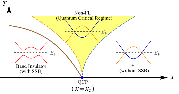
Figure 1: A phase diagram of the two-band fermion system coupled with U(1) symmetric $\phi^{4}$ boson: Eqs. (1,2,4). The vertical axis is temperature $T$, and horizontal axis $(x\sim m^{2}_{0})$ is a parameter that induces a quantum phase transition with the SSB of the U(1) symmetry. In the SSB phase, the Fermi system acquires a finite band gap, while in the U(1) symmetric phase, the Fermi system belongs to a multiple-band Fermi liquid (m-FL) phase. At the QCP and its high-$T$ side (QCR), the Fermi system shows a non-FL behaviour (See Table. 1).

	$C_{\rm el}/T$	$\chi_{\rm mag}$	$1/(T_{1}T)$	$\rho(\omega,T=0)$
non-Fermi liquid	$\frac{1}{\sqrt{|\ln T|}}$	$\frac{1}{\sqrt{|\ln T|}}$	$\frac{1}{|\ln T|}$	$\frac{1}{\sqrt{|\ln|\omega||}}$

Table 1: $T$-dependences of specific heat $C_{\rm el}$, and magnetic susceptibility $\chi_{\rm mag}$, and NMR relaxation time $T_{1}$ in the QCR and DOS near the Fermi level ($\omega=0$) at the QCP. For the magnetic response, we consider a trivial SU(2) generalization of Eqs. (1,2,4); $\psi_{\sigma}\rightarrow\psi_{\sigma,s}$, $\phi\psi^{\dagger}_{-}\psi_{+}\rightarrow\phi\psi^{\dagger}_{-,s}\psi_{+,s}$ with spin-1/2 $s=\uparrow,\downarrow$.

$$S_{\psi} =\sum_{\sigma=\pm}\int_{k}\psi^{\dagger}_{\sigma}(k)\big{[}i\omega-\sigma v_{\sigma 0}l\big{]}\psi_{\sigma}(k),$$ (2)

$$\int_{k} \equiv k^{2}_{F}\int\frac{d^{2}\hat{\Omega}}{(2\pi)^{2}}\int^{\overline{\Lambda}_{F}}_{-\overline{\Lambda}_{F}}\frac{d\omega}{2\pi}\int^{\Lambda_{F}}_{-\Lambda_{F}}\frac{dl}{2\pi}.$$ (3)

$k$ is fermion frequency and momentum; $k\equiv(\omega,{\bm{k}})$, ${\bm{k}}\equiv(k_{F}+l)\hat{\Omega}$. A unit vector $\hat{\Omega}$ defines a direction of ${\bm{k}}$ and a perpendicular component $l$ defines a vertical distance of ${\bm{k}}$ from the FS. $v_{+0}$ and $v_{-0}$ are bare fermion velocities of electron-type and hole-type; $v_{+0}>0$, $v_{-0}>0$. The free fermion part is described by a spatially isotropic free theory with the dynamical exponent $z=1$. $\Lambda_{F}$ and $\overline{\Lambda}_{F}$ are ultraviolet (UV) cutoff for $l$, and $\omega$. The boson field $\phi$ mediates a coupling between the two FSs in a U(1) symmetric way, $\phi\rightarrow\phi e^{+2i\theta},\psi^{\dagger}_{\pm}\rightarrow\psi^{\dagger}_{\pm}e^{\pm i\theta}$;

$$S_{\rm int} =g_{0}\int_{k}\int_{q}\big{[}\phi^{\dagger}(q)\psi^{\dagger}_{+}(k)\psi_{-}(k+q)+{\rm h.c.}\big{]},$$ (4)

$$\int_{q} \equiv\int_{|{\bm{q}}|<\Lambda_{B}}\frac{d^{3}{\bm{q}}}{(2\pi)^{3}}\int^{+\overline{\Lambda}_{B}}_{-\overline{\Lambda}_{B}}\frac{d\varepsilon}{2\pi}.$$ (5)

$g_{0}$ is nothing but a (bare) Yukawa coupling. In this paper, $k$ is always for the fermion ferquency and momentum and $q$ is boson frequency and momentum; $k\equiv(\omega,(k_{F}+l)\hat{\Omega})$, $q\equiv(\varepsilon,{\bm{q}})$. $\Lambda_{B}$ and $\overline{\Lambda}_{B}$ are UV cutoff for $q$ respectively.

In the paper, we will clarify how the Fermi system acquires a band gap when the boson system undergoes a quantum phase transition with the spontaneous symmetry breaking (SSB) of the U(1) symmetry. We show that the fermion’s DOS shows a pseudo-gap behaviour with a logarithmic energy dependence at the QCP and physical properties exhibit the logarithmic $T$-dependences in a high-temperature ($T$) side of the QCP: see Table. 1.

I.1 summary of this paper

The structure of the paper is as follows. In Sec. II, we introduce two concrete physical systems for which the effective action of Eqs. (1,2,4) is applicable. The first physical system is a 3-dimensional interacting Fermi system with a pair of electron and hole FSs with an excitonic instability. The intereacting Fermi system has a band inversion energy that measures an energy difference between the electron-band energy minimum and hole-band energy maximum. We discuss that when the band inversion energy is fine-tuned to a ‘frustrated’ point where the excitonic instability is maximally supressed, a quantum dielectric transition associated with the excitonic instability is characterized by the effective action given by Eqs. (1,2,4).

The second physical system is introduced on a cubic lattice; a quantum rotor model (QRM) coupled with a two-band free-fermion model. The QRM comprises of a U(1) phase variable $\theta_{\bm{j}}$ and its canonical conjugate momentum $L_{\bm{j}}$, defined on the cubic lattice site ${\bm{j}}$. For a heavier mass of the quantum rotor, the boson model undergoes a quantum phase transition to a long-range ordering of the U(1) phase variable. The free-fermion model is a tight-binding model on the cubic lattice, that has $s$ orbital ($s_{\bm{j}}$) and $p_{+}\equiv p_{x}+ip_{y}$ orbital ($p_{\bm{j}}$) on the same lattice site ${\bm{j}}$. The tight-binding model has a pair of electron and hole pockets around high symmetric points. We discuss that when the rotor is regarded as an electric/magnetic dipole moment, the simplest symmetry-allowed coupling between the rotor and the fermions in the tight-binding model is given by $e^{i\theta_{\bm{j}}}s^{\dagger}_{\bm{j}}p_{\bm{j}}$. Such an on-site coupling together with the QRM and the free-fermion model can be effectively described by Eqs. (1,2,4) near the quantum phase transition point.

In Sec. III, we give a general consideration on ground-state phase diagram and renormalizability of the effective model. For Eqs. (1,2,4) with the UV cutoff Eqs. (3,5), vertex functions (amputated 1-particle-irreducible part of connected Green functions) have potentially UV divergences in the power of the large UV cutoff $\Lambda$ ($\Lambda=\Lambda_{B},\overline{\Lambda}_{B},\Lambda_{F},\overline{\Lambda}_{F}$). The order of the UV divergence ($M$) of the vertex function $\Gamma^{(N_{F},N_{B})}$ with $N_{F}$ and $N_{B}$ external fermion and boson lines respectively can be superficially evaluated by dimensional countings and it is bounded from above by $M\leq 4-\frac{3}{2}N_{F}-N_{B}$ in the three-spatial dimension. That says, the effective model in the (3+1)-dimension is renormalizable, where only the following four vertex functions have the UV divergences in $\Lambda$;

$$\left\{\begin{array}[]{l}\Gamma^{(2,0)}_{\sigma}(i\omega,{\bm{k}})=\ldots\Lambda+\ldots\ln\Lambda\!\ i\omega+\ldots\ln\Lambda\!\ l,\\ \Gamma^{(0,2)}(i\varepsilon,{\bm{q}})=\ldots\Lambda^{2}+\ldots\ln\Lambda\!\ \varepsilon^{2}+\ldots\ln\Lambda\!\ {\bm{q}}^{2},\\ \Gamma^{(2,1)}_{\sigma}(\cdots)=\ldots\ln\Lambda+{\cal O}(\omega,l,q),\\ \Gamma^{(0,4)}(\cdots)=\ldots\ln\Lambda+{\cal O}(\omega,l,q).\\ \end{array}\right.$$ (10)

Here the subscript $\sigma=\pm$ is a band index, that distinguishes different functions for the same $N_{F}$ and $N_{B}$. Thereby, we use the standard renormalized perturbation theory, and eliminate all the UV divergences in Eq. (10) by absorbing them into renormalizations of field operator amplitudes, and physical measurable quantities.

The effective model in Eqs. (1,2,4) assumes that $q,\omega,l\ll\Lambda\ll k_{F}$. By the renormalized perturbation theory, the set of renormalized vertex functions shall be free from the UV cutoff $\Lambda$; the $\Lambda$-divergent terms in Eq. (10) are absorbed into the renormalizations of the physical quantities and field operator amplitudes, while $q/\Lambda$, $\omega/\Lambda$, $l/\Lambda$ are set to zero in the renormalized functions. On the one hand, the renormalized vertex functions thus obtained depend not only on $q$, $\omega$, $l$ but also on $k_{F}$. In Sec. III, we shall also argue that such an exceptional treatement of $k_{F}$ in spite of $q,\omega,l\ll\Lambda\ll k_{F}$ becomes possible, because all the vertex functions in Eq. (10) can be expanded in the power of $k^{2}_{F}$. To be more specific, we show that the vertex functions for $N_{F}=0,2$ can be expanded in the power of $k^{2}_{F}$; $\Gamma^{(N_{F},N_{B})}=\Gamma^{(N_{F},N_{B};0)}+k^{2}_{F}\Gamma^{(N_{F},N_{B};1)}+\cdots$, where $k^{2n}_{F}\Gamma^{(N_{F},N_{B};n)}$ is a sum of all those amputated 1-particle irreducible (1PI) Feynman diagrams for $\Gamma^{(N_{F},N_{B})}$ with $n$ numbers of internal closed fermion loops. Importantly, $\Gamma^{(N_{F},N_{B};n)}$ has no $k_{F}$-dependence and their $k_{F}$-dependence appear only through the overall factor $k^{2n}_{F}$. Thanks to this analytic nature as functions of $k^{2}_{F}$, the UV divergences in Eq. (10) can be removed at every order in $k^{2}_{F}$. In $\Gamma^{(N_{F},N_{B};n)}$ thus given, the superficial degree of the UV divergence in the power of $\Lambda$ is smaller than that of $\Gamma^{(N_{F},N_{B};0)}$ by $2n$. Accordingly, we have only to keep track of the first order in $k^{2}_{F}$ of $\Gamma^{(0,2)}$.

In Sec. IV, we shall eliminate the UV divergences in all the vertex functions in Eq. (10), while including the UV cutoff dependences into the renormalization of the field operators amplitudes and physical quantities. To this end, we impose the following renormalization conditions on the renormalied vertex function $\overline{\Gamma}^{(N_{F},N_{B})}$;

$$\left\{\begin{array}[]{l}\overline{\Gamma}^{(2,0)}_{\sigma}(\omega=l=0)=0,\!\ \frac{\partial\overline{\Gamma}^{(2,0)}_{\sigma}(\omega,l)}{\partial(i\omega)}\Big{|}_{v_{\sigma}l=0,\omega=\kappa}=1,\\ \frac{\partial\overline{\Gamma}^{(2,0)}_{\sigma}(\omega,l)}{\partial(v_{\sigma}l)}\Big{|}_{v_{\sigma}l=\kappa,\omega=0}=-\sigma,\\ \overline{\Gamma}^{(0,2)}(\varepsilon=\kappa,{\bm{q}}=0)=m^{2}+\kappa^{2},\\ \frac{\partial\overline{\Gamma}^{(0,2)}(q)}{\partial\varepsilon}\Big{|}_{{\bm{q}}=0,\varepsilon=\kappa}=2\kappa+\frac{g^{2}}{\pi^{2}(v_{+}+v_{-})}\frac{k^{2}_{F}}{\kappa}\\ \frac{\partial\overline{\Gamma}^{(0,2)}(q)}{\partial(c|{\bm{q}}|)}\Big{|}_{c|{\bm{q}}|=\kappa,\varepsilon=0}=2\kappa+\frac{g^{2}}{\pi^{2}(v_{+}+v_{-})}\frac{k^{2}_{F}}{\kappa},\\ \overline{\Gamma}^{(2,1)}_{\sigma}(\cdots)=-g,\!\ \overline{\Gamma}^{(0,4)}(\cdots)=-\lambda,\\ \end{array}\right.$$ (17)

with $\sigma=\pm$. $\kappa$ in Eq. (17) is an external momentum and frequency of the functions, at which the conditions are imposed. The right hand sides of Eq. (17) are free from the UV cutoff $\Lambda$, and they depend only on physical measurable quantities, such as renormalized boson mass $m$, renormalized Fermi velocities $v_{\pm}$, boson velocity $c$, and renormalized coupling constants $g$, $\lambda$. When the renormalized mass is set to the zero (at the critical point), a finite ‘$\kappa$’ controls infrared behaviours of the vertex functions.

In sec. IV, we employ the minimal substraction scheme Peskin and Schroeder (1995); Amit and Martin-Mayor (2005), to make the renormalized vertex functions to satisfy the renormalization conditions perturbatively in the coupling constants, $g$ and $\lambda$. The perturbative treatment will be a posteriori justified by $\beta$-functions of $g$ and $\lambda$ (see below). A general relation among numbers of internal integral variables, $g$ and $\lambda$ in a vertex function suggests that $g^{2}$ and $\lambda$ should be treated as the same order (Eq. (103) in Sec. III). Under Eq. (17), all the UV divergences in the vertex functions in Eq. (10) are absorbed into bare quantities ($v_{\sigma 0}$, $m^{2}_{0}$, $c_{0}$, $g_{0}$, $\lambda_{0}$) and renormalizations of field operator amplitudes ($Z_{\sigma}$, $Z_{\phi}$). At the quantum critical point with $m=0$, the bare quantities thus determined are given by

$$v_{\sigma 0} =v_{\sigma}+\frac{g^{2}(v_{\sigma}-c)}{4\pi^{2}c^{2}(c+v_{\overline{\sigma}})}\log\Big{(}\frac{\Lambda_{B}}{\kappa}\Big{)}+\cdots,$$ (18)

$$Z_{\sigma} =1-\frac{g^{2}}{4\pi^{2}c^{2}(c+v_{\overline{\sigma}})}\log\Big{(}\frac{\Lambda_{B}}{\kappa}\Big{)}+\cdots,$$ (19)

$$m^{2}_{0} =\frac{g^{2}k^{2}_{F}}{\pi^{2}(v_{+}+v_{-})}\log\Big{(}\frac{\Lambda_{F}}{\kappa}\Big{)}-\frac{\lambda\Lambda^{2}_{B}}{16\pi^{2}c^{3}}+\cdots,$$ (20)

$$g_{0} =g+\frac{g^{3}}{8\pi^{2}c^{2}}\frac{2c+v_{+}+v_{-}}{(c+v_{+})(c+v_{-})}\log\Big{(}\frac{\Lambda_{B}}{\kappa}\Big{)}+\cdots,$$ (21)

$$\lambda_{0} =\lambda+\frac{5\lambda^{2}}{16\pi^{2}c^{3}}\log\Big{(}\frac{\Lambda_{B}}{\kappa}\Big{)}+\cdots,$$ (22)

with $c_{0}=c+\cdots$, $Z_{\phi}=1+\cdots$, $\overline{\sigma}=\mp$ for $\sigma=\pm$. Here only the leading order terms in $g^{2}$ and $\lambda$ that depend on either $\Lambda$ or $\kappa$ are shown explicitly in the right hand sides, while the others are omitted by ‘$\cdots$’. The renormalized vertex functions defined by renormalized field operators, $\overline{\psi}_{\sigma}\equiv\psi_{\sigma}/\sqrt{Z_{\sigma}}$, $\overline{\phi}\equiv\phi/\sqrt{Z_{\phi}}$, are free from the UV cutoff as functions of the renormalized physical quantities. Note that Eq. (20) defines a subspace of $m=0$ (quantum critical ‘point’) in a multiple-parameter space subtended by the bare quantities and $\ln\kappa$. When $m=0$, the external momenta $\kappa$ plays role of a renormalization group (RG) scale variable and all the $\log\Lambda$ in the above equations come in pairs with $-\log\kappa$.

In Sec. V, we clarify non-FL features in the renormalized two-point fermion function around quantum critical point. To this end, we first derive a Callan-Symmanzik (CS) equation for the renormalized two-point fermion vertex function;

$$\Big{\{}\frac{\partial}{\partial\ln\kappa}+\sum_{\sigma^{\prime}=\pm}\beta_{v_{\sigma^{\prime}}}\frac{\partial}{\partial v_{\sigma^{\prime}}}+\beta_{g}\frac{\partial}{\partial g}+\beta_{\lambda}\frac{\partial}{\partial\lambda}$$

$$\ \ \ \ -\gamma_{\sigma}\Big{\}}\overline{\Gamma}^{(2,0)}_{\sigma}(l,\omega;c,\cdots,\lambda,\kappa)=0,$$ (23)

together with $\beta$ functions of Fermi velocities, and coupling constants,

$$\left\{\begin{array}[]{l}\beta_{v_{\sigma}}\equiv\frac{\partial v_{\sigma}}{\partial\ln\kappa}\Big{|}_{c_{0},\cdots,\Lambda}=\frac{g^{2}}{4\pi^{2}c(c+v_{\overline{\sigma}})}\Big{(}\frac{v_{\sigma}}{c}-1\Big{)}+\cdots,\\ \beta_{g}\equiv\frac{\partial g}{\partial\ln\kappa}\Big{|}_{c_{0},\cdots,\Lambda}=\frac{g^{3}}{8\pi^{2}c^{2}}\Big{(}\frac{1}{c+v_{+}}+\frac{1}{c+v_{-}}\Big{)}+\cdots\\ \beta_{\lambda}\equiv\frac{\partial\lambda}{\partial\ln\kappa}\Big{|}_{c_{0},\cdots,\Lambda}=\frac{5\lambda^{2}}{16\pi^{2}c^{3}}+\cdots,\\ \end{array}\right.$$ (27)

and $\gamma$ functions of the two fermion bands ($\sigma=\pm$),

$$\gamma_{\sigma}\equiv\frac{\partial\ln Z_{\sigma}}{\partial\ln\kappa}\Big{|}_{c_{0},\cdots,\Lambda}=\frac{g^{2}}{4\pi^{2}c^{2}(c+v_{\overline{\sigma}})}+\cdots.$$ (28)

The $\beta$ functions of the velocities show that two Fermi velocities $v_{\pm}$ are renormalized into the boson velocity $c$ in the infrared (IR) limit ($\kappa\rightarrow 0$). This suggests that $v_{\pm}$ in the CS equation could be set to $c$ in the low-energy limit. $\beta$ functions of the coupling constants dictate that the two coupling constants are marginally irrelevant in the IR limit. The marginal irrelevance justifies a posteriori the perturbative treatment of the coupling constants. Besides, the $\lambda$-dependence of $\Gamma^{(2,0)}$ must start from the order of ${\cal O}(g^{2}\lambda)$, so that $\partial_{\lambda}$ in Eq. (23) leads to the higher-order terms, ${\cal O}(g^{2}\lambda^{2})$, and can be omitted. These simplifications lead to the homogeneous CS equation with a one-parameter scaling. The solution of such CS equation is given in the form of the renormalized Green’s function with $\Gamma^{(2,0)}G^{(2,0)}=1$;

$$\overline{G}^{(2,0)}_{\sigma}(l,\omega;g,\kappa) =\frac{\exp\Big{[}-\int^{g}_{\overline{g}}\frac{\gamma_{\sigma}(g^{\prime})}{\beta_{g}(g^{\prime})}dg^{\prime}\Big{]}}{i\omega-\sigma cl}=\frac{\frac{\overline{g}(t)}{g}}{i\omega-\sigma cl}.$$ (29)

$\overline{g}(t)$ is a solution of the one-parameter scaling equation; $\partial\overline{g}/\partial t=\beta_{g}(\overline{g})$, $\overline{g}(t=0)=g$,

$$\overline{g}(t)=\frac{g}{\sqrt{1-2\alpha t}},\!\ \!\ \!\ \!\ t\equiv\log\bigg{[}\frac{\sqrt{\omega^{2}+(cl)^{2}}}{\kappa}\bigg{]},$$ (30)

with $\alpha\equiv g^{2}/(8\pi^{2}c^{3})$.

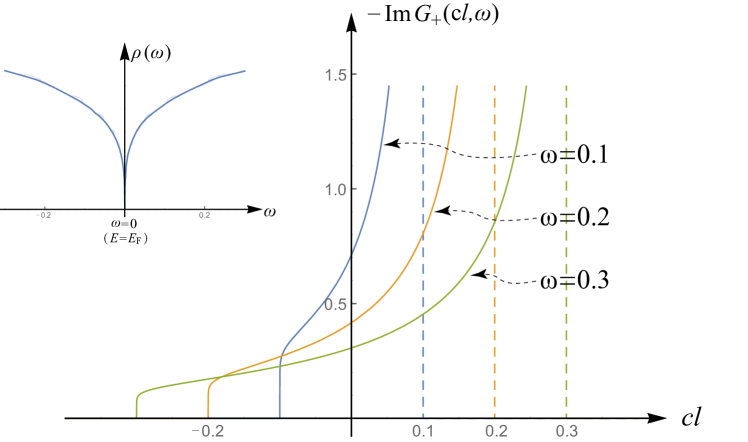
Figure 2: (a) Renormalized spectral function for the electron-type band at the QCP: $-{\rm Im}G^{R}_{+}(cl,\omega)$ is plotted as a function of $cl$ for $\omega=0.1,\!\ 0.2,\!\ 0.3$ with the RG scale $\kappa=1$. (inset) DOS at the QCP: $\rho(\omega)$.

In Sec. VI, we obtain fermion’s two-point retarded Green’s function, spectral function and DOS at the QCP (Fig. 2). After an analytic continuation, $i\omega\rightarrow\omega+i\delta$, Eq. (29) gives the retarded Green’s function. Thereby, it can be clearly seen from Eqs. (29,30) with $i\omega\rightarrow\omega+i\delta$ that the quasi-particle spectral weight at $T=0$ is zero because $\overline{g}/g$ in Eq. (29) goes to zero whenever $\omega\rightarrow\sigma cl$; ${\rm Re}\!\ t\rightarrow-\infty$. The vanishing quasi-particle spectral weight at the quantum critical point is the cornerstone of the non-Fermi liquid property in this paper. The spectral function comprises only of continuum spectrum, that shows an asymptotic form of $1/[\eta|\ln\eta|^{\frac{3}{2}}]$ when $\omega=\sigma(cl+\eta)$ with small positive $\eta$ (Fig. 2). The asymptotic form around $\omega=\sigma cl$ plays major role in the pseudo-gap behaviour of the DOS at the QCP; $\rho(\omega)\propto 1/|\ln|\omega||^{\frac{1}{2}}$ (inset of Fig. 2).

In Sec. VII, we conclude the paper with discussion on thermodynamic and magnetic properties of the two-band fermion system coupled with the critical $\phi^{4}$ bosons. In the appendix, we derive and solve the Callan-Symanzik equation for two-point boson Green functions and discuss the boson spectral function at the QCP.

II Physical Systems

As for conrete physical systems to which the effective model of Eqs. (1,2,4) is applicable, we consider the two systems: (i) a three-dimensional (3D) interacting two-bands fermion system with an excitonic instability, and (ii) multiple-band electron model coupled with quantum rotor model with/without an $Z_{n}$ anisotropy term ($n\geq 4$).

II.1 excitonic condensations in interacting two-bands fermion systems at a ‘frustrated’ point

Consider a 3D two-band interacting spinless fermion model with an excitonic instability. A partition function for the excitonic-pairing order parameter can be given by

$$Z =\int{\cal D}a{\cal D}b{\cal D}\Phi\!\ {\rm exp}\Big{[}-\int^{\beta}_{0}d\tau\int d^{3}{\bm{x}}\Big{\{}a^{\dagger}\partial_{\tau}a+b^{\dagger}\partial_{\tau}b$$

$$\hskip 28.45274pt-\mu_{E}(a^{\dagger}a-b^{\dagger}b)-\mu_{0}(a^{\dagger}a+b^{\dagger}b)$$

$$\hskip 28.45274pt+H_{el}(a,b)+a^{\dagger}b\Phi+b^{\dagger}a\Phi^{*}-\frac{1}{g}|\Phi|^{2}\Big{\}}\Big{]}$$ (31)

$$=\int{\cal D}\Phi\!\ {\rm exp}\Big{[}-\int^{\beta}_{0}d\tau\int d^{3}{\bm{x}}\Big{\{}u\Phi^{*}\partial_{\tau}\Phi+v|\partial_{\tau}\Phi|^{2}$$

$$\hskip 22.76228pt+w|\partial_{\bm{x}}\Phi|^{2}+A|\Phi|^{2}+B(|\Phi|^{2})^{2}+\cdots\Big{\}}\Big{]}.$$ (32)

Here $H_{el}(a,b)$ is a free (kinetic energy) part of the two-bands electron systems. $a$ and $b$ are field operators of the $a$-band (electron-type) fermion and $b$-band (hole-type) fermion respectively. $\mu_{E}$ and $\mu_{0}$ are ‘staggered’ and uniform chemical potential. The staggered chemical potential $\mu_{E}$ is nothing but an energy difference between the electron-band energy minimum and the hole-band energy maximum (Fig. 3(a)). We call this as ‘band inversion energy’.

A repulsive interaction between the two fermions is decomposed into a coupling between an excitonic pairing field $\Phi$, and the two fermion field operators. After an integration of the fermion fields, one would obtain the $(3+1)$D $\phi^{4}$-type effective action for the excitonic field, that varies slowly in space and time (see Eq. (32)). In the absence of the Berry phase term $\Phi^{*}\partial_{\tau}\Phi$ ($u=0$), such an effective action becomes identical to the boson part of the effective model with $z=1$ studied in this paper; Eq. (1). A coefficient for the Berry phase term, $u$, as well as others ($v$, $A$, $w$, $\cdots$) depend on microscopic parameters such as $\mu_{E}$ and other parameter $x$;

$$u(\mu_{E},x,\cdots),\ \ v(\mu_{E},\cdots),\ \ A(\mu_{E},\cdots),\cdots.$$

In general, $u$ is finite, and thus the dynamical exponent $z$ of the boson part of the action is $2$. Nonetheless, the linear coefficient $u$ can be exactly zero when $\mu_{E}$ is fine-tuned at a certain point, say $\mu_{E}=\mu_{E,f}$,

$$u(\mu_{E}=\mu_{E,f},\cdots)=0,\ \ v(\mu_{E}=\mu_{E,f},\cdots)>0,$$ (33)

where $z=1$. A quantum phase transition at such fine-tuned point ($\mu_{E}=\mu_{E,f}$), that is driven by the other parameter $x$, is effectively well described by the fermion-boson coupled model studied in this paper, Eqs. (1,2,4).

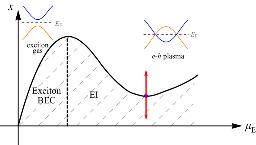
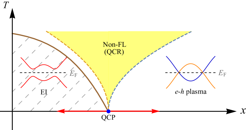
Figure 3: a: (upper) A schematic ground state phase diagram of an interacting two-bands fermion model in the 3 spatial dimension of Eq. (31). The phase diagram is subtended by a band inversion parameter $\mu_{E}$ and other parameter $x$. The excitonic phase with the broken U(1) symmetry is identified by a region of $A<0$ in Eq. (32), while the U(1) symmetric normal phase can be identified by the other region of $A>0$. The phase boundary between these two regions is defined by $x=X(\mu_{E})$. We fine-tune $\mu_{E}$ at those values of $\mu_{E}$ where $X$ have local minima, say $\mu_{E}=\mu_{E,f}$. A quantum phase transition driven by the other parameter $x$ at $\mu_{E}=\mu_{E,f}$ can be well described by the effective model studied in this paper. b: (lower) A schematic $T$-$x$ phase diagram associated with the quantum phase transition at $\mu_{E}=\mu_{E,f}$. The non-FL region is expected in a yellow colored region.

To identify such fine-tuned critical point for $\mu_{E}$, we follow an argument based on a local gauge symmetry Fisher et al. (1989). To this end, note first that Eq. (31) is invariant under the following local gauge transformation;

$$a^{\dagger}\rightarrow a^{\dagger}e^{i\frac{\theta(\tau)}{2}},\ b^{\dagger}\rightarrow b^{\dagger}e^{-i\frac{\theta(\tau)}{2}},$$

$$\Phi\rightarrow\Phi e^{-i\theta(\tau)},\ \mu_{E}\rightarrow\mu_{E}-i\frac{\partial_{\tau}\theta}{2}.$$ (34)

So is Eq. (32). Thus, for sufficiently small $\partial_{\tau}\theta(\tau)$, we could expand Eq. (32) and $u$, $v$ and $A$ in the power of $\partial_{\tau}\theta$, where the variation must be zero. This gives the following general relations,

$$\frac{1}{2}\frac{\partial A}{\partial\mu_{E}}=u,\ \ \frac{1}{2}\frac{\partial u}{\partial\mu_{E}}=-2v.$$ (35)

With Eq. (35) in mind, consider a $T=0$ phase diagram of the interacting two-bands fermion system. For simplicity, we consider a two-dimensional phase diagram subtended by $\mu_{E}$ and $x$ (Fig. 3). In the $T=0$ phase diagram, a region with $A<0$ could be regarded as an excitonic phase with the SSB of the global U(1) symmetry ($|\Phi|\neq 0$), while the other region with $A>0$ can be regarded as a U(1) symmetric normal phase ($|\Phi|=0$). A phase boundary between these two regions is denoted by $x=X(\mu_{E})$. From Eq. (35), one can see the minima of $X$ as a function of $\mu_{E}$ are the desired fine-tuned critical points with $u=0$ and $v>0$;

$$\left\{\begin{array}[]{lcc}u=0,&v<0,&\!\ \!\ {\rm for}\!\ \!\ \frac{dX}{d\mu_{E}}=0\!\ \cap\!\ \frac{d^{2}X}{d\mu^{2}_{E}}<0,\\ u=0,&v>0,&\!\ \!\ {\rm for}\!\ \!\ \frac{dX}{d\mu_{E}}=0\!\ \cap\!\ \frac{d^{2}X}{d\mu^{2}_{E}}>0.\\ \end{array}\right.$$ (38)

Since the excitonic phase is suppressed as a function of $x$ at the fine-tuned points, we call such fine-tuned values of $\mu_{E,f}$ as ‘frustrated’ points with maximally suppressed excitonic instability.

II.2 $sp$ model coupled with a quantum rotor model

The second physical system is a quantum rotor model coupled with two-orbital spinless fermion model. The fermion part is introduced on a 3D cubic lattice. Each lattice points has $s$-orbital and $p_{+}\equiv p_{x}+ip_{y}$ orbital degree of freedom of the spinless fermion. The fermion Hamiltonian is described by a two-orbital tight-binding model;

$$H_{\rm sp}\equiv\sum_{{\bm{j}},{\bm{m}}}\sum_{\alpha,\beta=s,p}[\mathbb{H}]_{({\bm{j}},\alpha|{\bm{m}},\beta)}c^{\dagger}_{{\bm{j}},\alpha}c_{{\bm{m}},\beta}$$

$$\equiv\sum_{\bm{j}}\bigg{\{}\Delta_{0}\Big{(}-s^{\dagger}_{\bm{j}}s_{\bm{j}}+p^{\dagger}_{\bm{j}}p_{\bm{j}}\Big{)}-t_{s}\sum_{\mu=x,y,z}\Big{(}s^{\dagger}_{{\bm{j}}+\mu}s_{\bm{j}}+{\rm h.c.}\Big{)}$$

$$+t_{p}\Big{(}p^{\dagger}_{{\bm{j}}+x}p_{\bm{j}}+p^{\dagger}_{{\bm{j}}+y}p_{\bm{j}}+{\rm h.c.}\Big{)}-t^{\prime}_{p}\Big{(}p^{\dagger}_{{\bm{j}}+z}p_{\bm{j}}+{\rm h.c.}\Big{)}$$

$$+t_{sp}\Big{(}(s^{\dagger}_{{\bm{j}}+x}+is^{\dagger}_{{\bm{j}}+y}-s^{\dagger}_{{\bm{j}}-x}-is^{\dagger}_{{\bm{j}}-y})p_{\bm{j}}+{\rm h.c.}\Big{)}\bigg{\}},$$ (39)

with ${\bm{j}}\equiv(j_{x},j_{y},j_{z})$, $x\equiv(1,0,0)$ and so on. Here all the intra-orbital hopping integrals $t_{s}$, $t_{p}$, $t^{\prime}_{p}$ as well as charge energy $\Delta_{0}$ are positive. When $t^{\prime}_{p}$ is chosen to be a negative value and the others are positive, the model becomes a prototype model for a magnetic Weyl semimetal and layered Chern insulator Yang et al. (2011); Chen et al. (2015); Liu et al. (2016).

In this work, we take $t_{s}=t^{\prime}_{p}=t_{p}=t>0$ and $t_{sp}=t^{\prime}$ for simplicity. The two energy bands are always separated by finite direct band gap;

$$E_{\pm}({\bm{k}})=-2tc_{z}\pm\sqrt{(\Delta_{0}+2t(c_{x}+c_{y}))^{2}+4{t^{\prime}}^{2}(s^{2}_{x}+s^{2}_{y})},$$

with $c_{x}\equiv\cos k_{x}$, $s_{x}\equiv\sin k_{x}$ and so on. When $\Delta_{0}-4t>0$, an upper energy band $E_{+}$ has an energy miminum at $(k_{x},k_{y},k_{z})=(\pi,\pi,0)$ and the lower energy band $E_{-}$ has an energy maximum at $(k_{x},k_{y},k_{z})=(\pi,\pi,\pi)$. When the Fermi level is set to zero, the two bands form an electron pocket and hole pocket around these extremes respectively,

$$E_{\pm}= \pm\Big{(}-2t+(\Delta_{0}-4t)+t(k^{2}_{x}+k^{2}_{y}+k^{2}_{z})$$

$$\ \ +\frac{2t^{\prime}}{\Delta_{0}-4t}(k^{2}_{x}+k^{2}_{y})\Big{)}+\cdots.$$

Note that a Fermi surface (FS) of the electron pocket around $(\pi,\pi,0)$ and that of the hole pocket around $(\pi,\pi,\pi)$ are identical in shape and size; $\mu=0$ is the charge-neutrality point. When $\Delta_{0},t\gg t^{\prime}$, the FS can be approximated by an isotropic Fermi surface and the two-orbital spinless fermion model can be well described by Eq. (2). Thereby, the electron and hole pockets are primarily composed of $p$ orbital and $s$ orbital respectively. In Eq. (39), a mixing is induced only by small $t^{\prime}$.

The boson part takes a form of quantum rotor model on the same cubic lattice with a $Z_{4}$ anisotropy Sachdev (1999),

$$H_{\rm qrm}=\frac{\hat{L}^{2}_{\bm{j}}}{2M}-J_{0}\sum_{\mu=x,y}\sum_{\bm{j}}\cos(\hat{\theta}_{\bm{j}}-\hat{\theta}_{{\bm{j}}+\mu})$$

$$\ \ +J_{\perp}\sum_{\bm{j}}\cos(\hat{\theta}_{\bm{j}}-\hat{\theta}_{{\bm{j}}+z})-\Delta_{4}\sum_{\bm{j}}\cos(4\hat{\theta}_{\bm{j}})$$ (40)

with $J_{0}$, $J_{\perp}$, $\Delta_{4}>0$. $\theta_{\bm{j}}$ represents a rotor degree of freedom defined on the cubic lattice site, taking a form of the U(1) phase variable. $\Delta_{4}$ is the $Z_{4}$ anisotorpy term that locks the rotor into four directions within a plane; $\theta_{{\bm{j}}}$ to $0,\pm\frac{\pi}{2},\pi$. The positive $J_{0}$ and $J_{\perp}$ favor an antiferro-type order of the U(1) phase variable; $\theta_{\bm{j}}$ orders in the ferro-type way within a $xy$ plane of the cubic lattice, and it orders in the antiferro-type way along the $z$ axis. $\hat{L}_{\bm{j}}$ is a momentum canonically conjugate to $\theta_{\bm{j}}$;

$$\big{[}\hat{\theta}_{\bm{j}},\hat{L}_{\bm{m}}\big{]}=i\hbar\delta_{{\bm{j}},{\bm{m}}}.$$ (41)

$M$ stands for a mass of the rotor. Larger $M$ reduces a kinetic energy of the rotor, favoring the ordering of the U(1) phase variable, while smaller $M$ induces a quantum phase transition from the antiferro-type order to a quantum disorder phase. In the quantum disorder phase, the momentum takes the definite integer value at every site, $L_{\bm{j}}=0$. Since the $Z_{4}$ anisotropy term is (dangerously) irrelevant at the quantum critical point José et al. (1977), the quantum phase transition is well described by the $(3+1)$-dimensional $\phi^{4}$ action with $z=1$ as in Eq. (1), where $e^{i\hat{\theta}_{\bm{j}}}(-1)^{j_{z}}$ plays role of a slowly-varying $\phi({\bm{x}})$ in Eq. (1) with ${\bm{j}}\equiv(j_{x},j_{y},j_{z})$ being identified with ${\bm{x}}$ Sachdev (1999).

II.2.1 coupling between rotor and $sp$ model

In this subsection, we shall introduce the most natural symmetry-allowed on-site coupling between the rotor and two-orbital spinless fermions. To this end, note first that the fermion model respects a magnetic point group symmetry of $4/mm^{\prime}m^{\prime}$, whose group elements are

$$C^{z}_{4},R\sigma_{x},R\sigma_{y},I,$$ (42)

and their combinations. Here $C^{z}_{4}$ is $\pi/2$ rotation around the $z$-axis, $R$ is the time-reversal operation, $\sigma_{x}$, $\sigma_{y}$ are mirror with respect to the $x=0$ and $y=0$ plane respectively, $I$ is the spatial inversion. Namely, the tight-binding Hamiltonian respects the following symmetries;

$$[\mathbb{H}]_{(C^{z}_{4}({\bm{j}})|C^{z}_{4}({\bm{m}}))}=\left(\begin{array}[]{cc}1&0\\ 0&-i\\ \end{array}\right)[\mathbb{H}]_{({\bm{j}}|{\bm{m}})}\left(\begin{array}[]{cc}1&0\\ 0&+i\\ \end{array}\right)\ :\!\ C^{z}_{4},$$ (47)

$$[\mathbb{H}^{T}]_{(\sigma_{x}({\bm{j}})|\sigma_{x}({\bm{m}}))}=\left(\begin{array}[]{cc}1&0\\ 0&-1\\ \end{array}\right)[\mathbb{H}]_{({\bm{j}}|{\bm{m}})}\left(\begin{array}[]{cc}1&0\\ 0&-1\\ \end{array}\right)\ :\!\ R\sigma_{x},$$ (52)

$$[\mathbb{H}^{T}]_{(\sigma_{y}({\bm{j}})|\sigma_{y}({\bm{m}}))}=[\mathbb{H}]_{({\bm{j}}|{\bm{m}})}\ :\!\ R\sigma_{y},$$

$$[\mathbb{H}]_{(I({\bm{j}})|I({\bm{m}}))}=\left(\begin{array}[]{cc}1&0\\ 0&-1\\ \end{array}\right)[\mathbb{H}]_{({\bm{j}}|{\bm{m}})}\left(\begin{array}[]{cc}1&0\\ 0&-1\\ \end{array}\right)\ :\!\ I.$$ (57)

In other words, Eq. (39) is invariant under the following transformations of the creation and annihilation operators of $s$ and $p$ orbitals,

$$\left(\begin{array}[]{c}s\\ p\\ \end{array}\right)\rightarrow\left(\begin{array}[]{cc}1&0\\ 0&+i\\ \end{array}\right)\left(\begin{array}[]{c}s\\ p\\ \end{array}\right)\ :\!\ C^{z}_{4},$$ (64)

$$\left(\begin{array}[]{c}s\\ p\\ \end{array}\right)\rightarrow\left(\begin{array}[]{cc}s^{\dagger}&p^{\dagger}\\ \end{array}\right)\left(\begin{array}[]{cc}1&0\\ 0&-1\\ \end{array}\right)\ :\!\ R\sigma_{x},$$ (70)

$$\left(\begin{array}[]{c}s\\ p\\ \end{array}\right)\rightarrow\left(\begin{array}[]{cc}s^{\dagger}&p^{\dagger}\\ \end{array}\right)\ :\!\ R\sigma_{y},$$ (74)

$$\left(\begin{array}[]{c}s\\ p\\ \end{array}\right)\rightarrow\left(\begin{array}[]{cc}1&0\\ 0&-1\\ \end{array}\right)\left(\begin{array}[]{c}s\\ p\\ \end{array}\right)\ :\!\ I$$ (81)

with $C^{z}_{4}(A_{({\bm{j}},\alpha|{\bm{m}},\beta)}c^{\dagger}_{{\bm{j}},\alpha}c_{{\bm{m}},\beta})=A_{\cdots}C^{z}_{4}(c^{\dagger}_{{\bm{j}},\alpha})C^{z}_{4}(c_{{\bm{m}},\beta})$, $I(Ac^{\dagger}_{{\bm{j}},\alpha}c_{{\bm{m}},\beta})=AI(c^{\dagger}_{{\bm{j}},\alpha})I(c_{{\bm{m}},\beta})$, and $R\sigma_{\mu}(Ac^{\dagger}_{{\bm{j}},\alpha}c_{{\bm{m}},\beta})=AR\sigma_{\mu}(c_{{\bm{m}},\beta})\!\ R\sigma_{\mu}(c^{\dagger}_{{\bm{j}},\alpha})$.

In the following, we introduce an on-site coupling between the two-orbital fermions and the quantum rotor, that respects all (or part of) these magnetic point group symmetry operations. To do so, we consider two physical cases, (i) when the rotor on each site has the same symmetry as $x$ and $y$-components of electric dipole; $e^{i\theta_{\bm{j}}}\sim E_{x}({\bm{j}})+iE_{y}({\bm{j}})$, and (ii) when the rotor has the same symmetry as the $x$ and $y$-components of magnetic dipole; $e^{i\theta_{\bm{j}}}\sim B_{x}({\bm{j}})+iB_{y}({\bm{j}})$.

II.2.2 when rotor is electric dipole

Consider the first case, where real and imaginary part of $e^{i\theta_{\bm{j}}}$ has the same symmetry as the $x$ and $y$ components of the electric dipole moment defined at ${\bm{j}}$ respectively. Under the symmetry operations of $4/mm^{\prime}m^{\prime}$, the rotor degree of freedom will be transformed as follows,

$$e^{i\theta_{\bm{j}}}\rightarrow e^{i(\theta_{\bm{j}}+\frac{\pi}{2})}\ :\!\ C^{z}_{4},\ \ e^{i\theta_{\bm{j}}}\rightarrow e^{i\theta_{\bm{j}}}\ :\!\ R,$$

$$e^{i\theta_{\bm{j}}}\rightarrow e^{-i\theta_{\bm{j}}}\ :\!\ \sigma_{y},\ \ e^{i\theta_{\bm{j}}}\rightarrow e^{i(\pi-\theta_{\bm{j}})}\ :\!\ \sigma_{x},$$

$$e^{i\theta_{\bm{j}}}\rightarrow-e^{i\theta_{\bm{j}}}\ :\!\ I,\ \ e^{i\theta_{\bm{j}}}\rightarrow-e^{-i\theta_{\bm{j}}}\ :\!\ R\sigma_{x},$$

$$e^{i\theta_{\bm{j}}}\rightarrow e^{-i\theta_{\bm{j}}}\ :\!\ R\sigma_{y}.\$$ (82)

Thus, the simplest on-site coupling between the electric dipole and the fermions that respects all the magnetic point group symmetry of $4/mm^{\prime}m^{\prime}$ is as follows,

$$H_{f-b}=\sum_{\bm{j}}\Big{(}e^{-i\hat{\theta}_{\bm{j}}}s^{\dagger}_{\bm{j}}p_{\bm{j}}+e^{i\hat{\theta}_{\bm{j}}}p^{\dagger}_{\bm{j}}s_{\bm{j}}\Big{)}.$$ (83)

In the presence of the on-site fermion-boson coupling, the slowly varying $\phi({\bm{x}}\simeq{\bm{j}})=e^{-i\hat{\theta}_{\bm{j}}}(-1)^{j_{z}}$ couples between the electron and hole pockets in the same form as in Eq. (4).

II.2.3 when rotor is magnetic dipole

Consider the second case, where real and imaginary part of $e^{i\theta_{\bm{j}}}$ has the same symmetry as the $x$ and $y$ components of the magnetic dipole moment defined at ${\bm{j}}$. Under the magnetic point group symmetry operations, the rotor degree of freedom will be transformed as follows,

$$e^{i\theta_{\bm{j}}}\rightarrow e^{i(\theta_{\bm{j}}+\frac{\pi}{2})}\ :\!\ C^{z}_{4},\ \ e^{i\theta_{\bm{j}}}\rightarrow-e^{i\theta_{\bm{j}}}\ :\!\ R,$$

$$e^{i\theta_{\bm{j}}}\rightarrow e^{i(\pi-\theta_{\bm{j}})}\ :\!\ \sigma_{y},\ \ e^{i\theta_{\bm{j}}}\rightarrow e^{-i\theta_{\bm{j}}}\ :\!\ \sigma_{x},$$

$$e^{i\theta_{\bm{j}}}\rightarrow e^{i\theta_{\bm{j}}}\ :\!\ I,\ \ e^{i\theta_{\bm{j}}}\rightarrow-e^{-i\theta_{\bm{j}}}\ :\!\ R\sigma_{x},$$

$$e^{i\theta_{\bm{j}}}\rightarrow e^{-i\theta_{\bm{j}}}\ :\!\ R\sigma_{y}.\$$ (84)

Thus the on-site coupling in Eq. (83) is symmetrically allowed by $C^{z}_{4}$, $R\sigma_{x}$ and $R\sigma_{y}$, while it is disallowed by $I$. In other words, the coupling of Eq. (4) is allowed by a subgroup of $4/mm^{\prime}m^{\prime}$: $4m^{\prime}m^{\prime}$. The group elements of the magnetic point group of $4m^{\prime}m^{\prime}$ are

$$C^{z}_{4},R\sigma_{x},R\sigma_{y},$$ (85)

and their combinations.

III Effective boson-fermion coupled model and its renormalizability

III.1 $(d+1)$-dimensional effective model and its ground-state phase diagram

The two physical systems discussed in the previous section can be described by Eqs. (1,2,4). To put it generally, consider the fermion-boson coupled system in the $(d+1)$-dimension,

$$S_{t}=S_{\psi}+S_{\phi}+S_{\psi-\phi},$$ (86)

$$S_{\psi}=\sum_{\sigma=\pm}\int\psi^{\dagger}_{\sigma}({\bm{x}},\tau)\big{[}\partial_{\tau}+\mu-E_{\sigma}(i\nabla)\big{]}\psi_{\sigma}({\bm{x}},\tau),$$ (87)

$$S_{\phi}=\!\ \int\big{[}m^{2}_{0}|\phi|^{2}+|\partial_{\tau}\phi|^{2}+c^{2}_{0}|{\bm{\nabla}}\phi|^{2}+\frac{\lambda_{0}}{4}\big{(}|\phi|^{2}\big{)}^{2}\big{]},$$ (88)

$$S_{\psi-\phi}=g_{0}\int\!\ \big{[}\phi^{\dagger}\psi^{\dagger}_{+}\psi_{-}+\phi\psi^{\dagger}_{-}\psi_{+}\big{]},$$ (89)

$$\int\equiv\int d\tau\int d^{d}{\bm{x}}.$$

The coupled system has global U(1) symmetries;

$$\left\{\begin{array}[]{l}{\rm(i)}\!\ \!\ \!\ \psi^{\dagger}_{\pm}\rightarrow\psi^{\dagger}_{\pm}e^{\pm i\theta},\ \ \psi_{\pm}\rightarrow\psi_{\pm}e^{\mp i\theta},\ \ \phi^{\dagger}\rightarrow\phi^{\dagger}e^{-2i\theta}.\\ {\rm(ii)}\!\ \!\ \!\ \psi^{\dagger}_{\pm}\rightarrow\psi^{\dagger}_{\pm}e^{i\theta},\ \ \psi_{\pm}\rightarrow\psi_{\pm}e^{-i\theta}.\\ \end{array}\right.$$ (92)

The kinetic energy of the free fermion part is isotropic in the $d$-dimensional space, and an momentum-energy dispersion for the two fermion bands depend only on a norm of momentum, $E_{\sigma}(|{\bm{k}}|)$ ($\sigma=\pm$). The two fermion’s energy bands are an electron-type band ($\sigma=+$) and hole-type band ($\sigma=-$) respectively. The chemical potential for the fermions is fine-tuned to a charge neutrality point (CNP), where the isotropic Fermi surface of the electron and that of the hole become identical to each other. The two momentum-energy dispersions are linearized around the isotropic Fermi surface. The fermion part is described by a free theory with the dynamical exponent $z=1$;

$$S_{\psi} =\int\frac{d^{d+1}k}{(2\pi)^{d+1}}\psi^{\dagger}_{+}(k)\big{[}i\omega-v_{+0}l\big{]}\psi_{+}(k)$$

$$\hskip 28.45274pt+\int\frac{d^{d+1}k}{(2\pi)^{d+1}}\psi^{\dagger}_{-}(k)\big{[}i\omega+v_{-0}l\big{]}\psi_{-}(k),$$

$$\equiv\sum_{\sigma=\pm}\int_{\Omega,\omega,l}\psi^{\dagger}_{\sigma}(k)\big{[}i\omega-\sigma v_{\sigma 0}l\big{]}\psi_{\sigma}(k),$$ (93)

and

$$\int_{k}\equiv k^{d-1}_{F}\int\frac{d^{d-1}\hat{\Omega}}{(2\pi)^{d-1}}\int^{\overline{\Lambda}_{F}}_{-\overline{\Lambda}_{F}}\frac{d\omega}{2\pi}\int^{\Lambda_{F}}_{-\Lambda_{F}}\frac{dl}{2\pi},$$ (94)

with $v_{+0}>0$, $v_{-0}>0$, $k\equiv(\omega,{\bm{k}})$ and ${\bm{k}}=(k_{F}+l)\hat{\Omega}$. $k_{F}$ is the Fermi wavelength of the isotropic Fermi surface and $l$ is the perpendicular component of the $d$-dimensional momentum, and $\hat{\Omega}$ is a unit vector in the $d$-dimensional momentum space. In the presence of the isotropic Fermi surface, the $d$-dimensional momentum integral is decomposed into one-dimensional integral over $l$ and $(d-1)$-dimensional integral over $\hat{\Omega}$. $\Lambda_{F}$ and $\overline{\Lambda}_{F}$ are high energy (ultraviolet) cutoff for the one-dimensional $l$-integral and the frequency ($\omega$) integral respectively.

The boson part and the coupling part of the action are given in the momentum-frequency space,

$$S_{\phi} =\int_{q}\big{(}m^{2}_{0}+c^{2}_{0}{\bm{q}}^{2}+\varepsilon^{2}\big{)}\phi^{\dagger}(q)\phi(q)$$

$$+\frac{\lambda_{0}}{4}\int_{q_{1},q_{2},q_{3}}\big{(}\phi^{\dagger}(q_{1})\phi(q_{2})\big{)}\big{(}\phi^{\dagger}(q_{3})\phi(q_{1}+q_{3}-q_{2})\big{)},$$ (95)

$$S_{\psi-\phi} =g_{0}\int_{k,q}\big{[}\phi^{\dagger}(q)\psi^{\dagger}_{+}(k)\psi_{-}(k+q)+{\rm h.c.}\big{]},$$ (96)

with $q\equiv(\varepsilon,{\bm{q}})$, $q_{j}\equiv(\varepsilon_{j},{\bm{q}}_{j})$ ($j=1,2,\cdots$), and

$$\int_{q}\equiv\int_{|{\bm{q}}|<\Lambda_{B}}\frac{d^{d}{\bm{q}}}{(2\pi)^{d}}\int^{\overline{\Lambda}_{B}}_{-\overline{\Lambda}_{B}}\frac{d\varepsilon}{2\pi},$$ (97)

$$\int_{k,q}\equiv\int_{k}\int_{q},\ \ \int_{q_{1},q_{2},q_{3}}\equiv\int_{q_{1}}\int_{q_{2}}\int_{q_{3}}.$$ (98)

Here $\Lambda_{B}$ and $\overline{\Lambda}_{B}$ are the ultraviolet (UV) cutoff for the boson momentum and frequency.

Figure 4: Polarization function in the interband channel. Two solid lines with arrow stand for the fermion Green’s function in particle and hole channel respectively. The dotted line stand for the boson Green’s function.

A ground-state phase diagram of the coupled system possibly comprises of two phases; the SSB phase with $\langle\psi^{\dagger}_{+}\psi_{-}\rangle\neq 0$ (band insulator phase) and U(1) symmetric phase (multiple-band FL phase). At the exact charge neutrality point (CNP), a polarization function in an interband channel (Fig. 4) has an infrared (IR) logarithmic singularity. The singularity in combination with any small Yukawa coupling $g_{0}$ could result in the low-$T$ band insulator phase with the SSB. A transition temperature $T_{c}$ is exponentially small for small $g_{0}$; $\log[T_{c}/\overline{\Lambda}_{F}]\propto-1/g^{2}_{0}$. In actual physical systems, however, the IR logarithmic singularity is weak enough that it is easily regularized by a tiny effect of other degree of freedom in low-energy scale. Such effects are disorder, an uncontrolled deviation from the CNP and/or spatially inhomegeneity of the carrier densities. Assuming these IR regularizations implicitly, we take it for granted the presence of the multiple-band FL phase and the quantum critical point (QCP) between the FL and the band insulator phases (Fig. 1). Thereby, the phase transition between the two is primarily driven by a change of the boson mass. In the following, we will uncover universal critical properties at such QCP and in a high-$T$ side of the QCP (quantum critical regime; QCR).

The Green’s and vertex functions play the central role in the characterizations of quantum criticality. Let us call as $\Gamma^{(N_{F},N_{B})}$ and $G^{(N_{F},N_{B})}$ the vertex and Green’s function respectively, that have $N_{F}$ external fermion lines and $N_{B}$ external boson lines. The Green functions are introduced together with the effective action $S_{t}$ as,

$$(2\pi)^{d+1}\delta^{d+1}(k-k^{\prime})\delta_{\sigma,\sigma^{\prime}}G^{(2,0)}_{\sigma}(k)\equiv\langle\psi_{\sigma}(k)\psi^{\dagger}_{\sigma^{\prime}}(k^{\prime})\rangle,$$

$$(2\pi)^{d+1}\delta^{d+1}(q-q^{\prime})G^{(0,2)}(q)\equiv\langle\phi(q)\phi^{\dagger}(q^{\prime})\rangle,$$

$$(2\pi)^{d+1}\delta^{d+1}(k^{\prime}-k-q)G^{(2,1)}_{+}(k,k+q;q)$$

$$\hskip 108.12054pt\equiv\langle\psi_{+}(k)\psi^{\dagger}_{-}(k^{\prime})\phi(q)\rangle,$$

$$(2\pi)^{d+1}\delta^{d+1}(k^{\prime}-k+q)G^{(2,1)}_{-}(k,k-q;q)$$

$$\hskip 108.12054pt\equiv\langle\psi_{-}(k)\psi^{\dagger}_{+}(k^{\prime})\phi^{\dagger}(q)\rangle,$$

$$(2\pi)^{d+1}\delta^{d+1}(q_{4}+q_{3}-q_{2}-q_{1})G^{(0,4)}(q_{1},q_{2},q_{3})$$

$$\hskip 91.04872pt\equiv\langle\phi(q_{4})\phi(q_{3})\phi^{\dagger}(q_{2})\phi^{\dagger}(q_{1})\rangle,$$ (99)

and

$$\langle\cdots\rangle \equiv\frac{1}{Z}\int D\phi^{\dagger}D\phi D\psi^{\dagger}D\psi\!\ e^{-S_{t}}\cdots,$$

$$Z \equiv\int D\phi^{\dagger}D\phi D\psi^{\dagger}D\psi\!\ e^{-S_{t}}.$$ (100)

Here the band index $\sigma,\sigma^{\prime}=\pm$ in Eq. (99) is an additional subscript, that distinguishes different functions for same $N_{F}$ and $N_{B}$. Because of the U(1) gauge symmetry Eq. (92), $G^{(2,1)}$ has only two different functions; $G^{(2,1)}_{\pm}$. $G^{(0,4)}$ comprises of connected and disconnected parts. The disconnected part is given by products of two $G^{(0,2)}$. The vertex functions are obtained from an amputation of the one-particle irreducible (1PI) parts of the connected Green’s functions;

$$G^{(2,0)}_{\sigma}(k)\Gamma^{(2,0)}_{\sigma}(k)\equiv 1,\ \ G^{(0,2)}(q)\Gamma^{(0,2)}(q)\equiv 1,$$

$$G^{(2,1)}_{\pm}(k,k\pm q;q)\equiv$$

$$\hskip 28.45274ptG^{(2,0)}_{\pm}(k)G^{(2,0)}_{\mp}(k\pm q)G^{(0,2)}(q)\Gamma^{(2,1)}_{\pm}(k,k\pm q;q),$$

$$G^{(0,4)}(q_{1},q_{2},q_{3})\equiv G^{(0,2)}(q_{1})G^{(0,2)}(q_{2})G^{(0,2)}(q_{3})$$

$$\hskip 22.76228pt\times G^{(0,2)}(q_{1}+q_{2}-q_{3})\Gamma^{(0,4)}(q_{1},q_{2},q_{3})+\cdots.$$ (101)

Here ‘$\cdots$’ in the last line stands for the disconnected part of $G^{(0,4)}$.

III.2 renormalizability

For the effective model of Eqs. (93,95,96), the vertex function $\Gamma^{(N_{F},N_{B})}$ has potentially an ultraviolet (UV) divergence in the power of a large UV cutoff $\Lambda$, which is either $\Lambda_{B}$, $\overline{\Lambda}_{B}$, $\Lambda_{F}$ or $\overline{\Lambda}_{F}$ defined in Eqs. (94,97,98). The degree of the UV divergence depends on the number of the external lines, $N_{F}$ and $N_{B}$, and the spatial dimension $d$. By the field theory, $\Gamma^{(N_{F},N_{B})}$ is given by a sum of amputated Feynman diagrams for the 1PI connected $G^{(N_{F},N_{B})}$. Each amputated Feynman diagram is given by an integral over $L$-number of internal $D$-dimensional momenta (frequency and momentum) with $D\equiv d+1$. The integrand is a product among $V_{F}$-number of internal fermion lines (fermion Green’s functions), $V_{B}$ internal boson lines (boson Green’s functions), $V_{1}$ vertices of the Yukawa couplings ($g_{0}$) and $V_{2}$ vertices of the $\phi^{4}$ coupling ($\lambda_{0}$). Such an integral can have a UV divergence with respect to the large UV cutoff $\Lambda$. The degree of the divergence can be superficially evaluated by a dimensional counting of the integral Peskin and Schroeder (1995); Amit and Martin-Mayor (2005). From the dimensional counting, the superficial degree of the UV divergence, $M$, is bounded from above by $D_{\rm max}=DL-V_{F}-2V_{B}$; $M\leq D_{\rm max}$. Here the equality holds true for those amputated Feynman diagrams which do not have any integrals over internal fermion momenta. The inequality applies for those Feynman diagrams which have the integrals over the internal fermion momenta (see also below). A sum of the internal and external boson lines in the connected $G^{(N_{F},N_{B})}$ is given by $V_{1}/2+2V_{2}+N_{B}/2\equiv V_{B}+N_{B}$, while a sum of the internal and external fermion lines is by $V_{1}+N_{F}/2\equiv V_{F}+N_{F}$. In terms of these two identities together with $L=V_{F}+V_{B}-V_{1}-V_{2}+1$, the dependences on $V_{F}$ and $V_{B}$ in $D_{\rm max}$ and $L$ can be eliminated,

$$D_{\rm max}= D+\frac{D-4}{2}V_{1}+(D-4)V_{2}$$

$$\ \ -\frac{D-1}{2}N_{F}-\frac{D-2}{2}N_{B},$$ (102)

and

$$L=\frac{V_{1}}{2}+V_{2}-\frac{N_{F}}{2}-\frac{N_{B}}{2}+1.$$ (103)

Eq. (102) suggests that $D=4$ ($d=3$) is an upper critical dimension, where the effective model of Eqs. (93,95,96) is renormalizable. Eq. (103) shows that for fixed $N_{E}$ and $N_{B}$, the number of the internal integral variables $L$ increases with a unit of either $V_{1}=2$ or $V_{2}=1$.

This paper focuses on the upper critical dimension of the effective model, where only the following four vertex functions have potentially the UV divergences at $D=4$,

$$\Gamma^{(2,0)},\!\ \Gamma^{(0,2)},\!\ \Gamma^{(2,1)},\!\ \Gamma^{(0,4)}.$$ (104)

From Eq. (102), their superficial degrees of the UV divergences in the power of the UV cutoff $\Lambda$ are evaluated (at most) $1$, $2$, $0$ and $0$ respectively. Note that both $\Gamma^{(1,0)}$, $\Gamma^{(0,1)}$ and $\Gamma^{(1,1)}$ are zero because of the gauge symmetries; Eq. (92). In the next section, we will use a renormalized perturbation theory and eliminate the dependences of the UV cutoff from these vertex functions by way of renormalizations of field operator amplitudes, boson mass, fermion velocities, boson velocity, Yukawa coupling and the $\phi^{4}$ coupling.

Before closing this section, let us explain how the Fermi wavelength $k_{F}$ is treated in this paper. The effective model implicitly assumes that the Fermi wavelength $k_{F}$ is much larger than the UV cutoff $\Lambda$ and the UV cutoff is much larger than fermion and boson momenta in Eqs. (93,95,96);

$$|{\bm{q}}|,\varepsilon,\omega,l\ll\Lambda_{B},\overline{\Lambda}_{B},\Lambda_{F},\overline{\Lambda}_{F}\ll k_{F}.$$ (105)

The renormalized theory shall be free from the UV cutoff $\Lambda$ (being $\Lambda_{B}$, $\overline{\Lambda}_{B}$, $\Lambda_{F}$ or $\overline{\Lambda}_{F}$), where $|{\bm{q}}|/\Lambda$, $\varepsilon/\Lambda$, $l/\Lambda$, $\omega/\Lambda$ are regarded as infinitesimally small and set to zero in the renormalized vertex functions. Meanwhile, we will allow the renormalized functions to depend not only on the boson and fermion momenta ${\bm{q}}$, $\varepsilon$, $\omega$, $l$ but also on the Fermi wavelength $k_{F}$. That says, the Fermi wavelength is treated as a finite (although the largest) measurable physical quantity.

To enable such an exceptional treatment of $k_{F}$ in spite of $|{\bm{q}}|$, $\varepsilon$, $\omega$, $l$ $\ll\Lambda$ $\ll k_{F}$, it is important to note that all the vertex functions in Eq. (104) can be expanded in the power of $k^{d-1}_{F}$;

$$\Gamma^{(N_{F},N_{B})}= \Gamma^{(N_{F},N_{B};0)}+k^{d-1}_{F}\Gamma^{(N_{F},N_{B};1)}$$

$$+k^{2(d-1)}_{F}\Gamma^{(N_{F},N_{B};2)}+\cdots,\!\ \!\ \!\ \!\ (N_{F}=0,2).$$ (106)

Here $k^{n(d-1)}_{F}\Gamma^{(N_{F},N_{B};n)}$ in the right hand side is a sum of all those amputated 1PI Feynman diagrams for $\Gamma^{(N_{F},N_{B})}$ that have $n$ numbers of internal closed loops formed by fermion lines (‘closed fermion loops’). Importantly, it has no $k_{F}$-dependence other than the overall factor, $k^{n(d-1)}_{F}$, for $N_{F}=0,2$. To see this, let us consider how to assign the $L$-number of the internal integral variables to the $(V_{F}+V_{B})$-number of the internal lines in an amputated 1PI Feynman diagram with $n$-number of the closed fermion loops. The most natural way of doing this in the case of $\Lambda\ll k_{F}$ is as follows. For each closed fermion loop, say the $j$-th closed fermion loop with $j=1,\cdots,n$, assign an integral variable of fermion momentum to one and only one internal fermion line in the loop, say $(\omega_{j},{\bm{k}}_{j})$ with ${\bm{k}}_{j}=(k_{F}+l_{j})\hat{\Omega}_{j}$. Meanwhile, assign the other $(L-n)$-number of the integral variables to the internal boson lines, such that momentum and frequency conservations are preserved at every vertex. The momenta of the other internal fermion lines in the $j$-th closed fermion loop shall be given by a sum of $(\omega_{j},{\bm{k}}_{j})$ and the boson momenta (either internal or external). For $N_{F}=2$ with an open fermion line with two external fermion points, one of the two external fermions is given by $(\omega,{\bm{k}})$, while the other external fermion is given by a sum of $(\omega,{\bm{k}})$ and external boson momenta (if any). Thereby, the momenta of the internal fermions in the open fermion line shall be given by a sum of the external fermion momentum $(\omega,{\bm{k}})$ and (either internal or external) boson momenta. With this way of the assignment of the integral variables, the integrand clearly has no $k_{F}$-dependence in the case of $\Lambda\ll k_{F}$. The only $k_{F}$-dependence in the integral appears through the overall factor, $k^{n(d-1)}_{F}$;

$$k^{n(d-1)}_{F}\Gamma^{(N_{F}\leq 2,N_{B};n)}= k^{n(d-1)}_{F}\sum_{L}\int\frac{d^{d-1}\hat{\Omega}_{1}}{(2\pi)^{d-1}}\int_{\Lambda}\frac{d\omega_{1}dl_{1}}{(2\pi)^{2}}\cdots\int\frac{d^{d-1}\hat{\Omega}_{n}}{(2\pi)^{d-1}}\int_{\Lambda}\frac{d\omega_{n}dl_{n}}{(2\pi)^{2}}$$

$$\hskip 79.6678pt\int_{\Lambda}\frac{d^{d+1}q_{1}}{(2\pi)^{d+1}}\cdots\int_{\Lambda}\frac{d^{d+1}q_{L-n}}{(2\pi)^{d+1}}\!\ \big{(}{\rm integrand}\!\ \!\ {\rm that}\!\ \!\ {\rm is}\!\ \!\ {\rm free}\!\ \!\ {\rm from}\!\ \!\ k_{F}\big{)}.$$ (107)

In $\Gamma^{(N_{F},N_{B};n)}$ thus given, the superficial degree of the UV divergence with respect to the power in $\Lambda$ is smaller than that of $\Gamma^{(N_{F},N_{B};0)}$ by $n(d-1)$.

$$\left\{\begin{array}[]{l}\big{[}\Gamma^{(N_{F},N_{B};0)}\big{]}=DL-V_{F}-2V_{B}\equiv D_{\rm max},\\ \big{[}\Gamma^{(N_{F},N_{B};1)}\big{]}=D_{\rm max}-(d-1),\\ \big{[}\Gamma^{(N_{F},N_{B};2)}\big{]}=D_{\rm max}-2(d-1),\ \ \cdots,\\ \big{[}\Gamma^{(N_{F},N_{B};n)}\big{]}=D_{\rm max}-n(d-1),\ \ \cdots.\\ \end{array}\right.$$ (112)

The integer in the right hand side refers to the superficial degree of the UV divergence in the left hand side. When the integer in the right hand side is less than $0$, the left hand side should be regarded as on the order of ${\cal O}(1)$ in the power of the UV cutoff $\Lambda$.

Thanks to the analytic feature of the vertex functions as functions of $k_{F}$, Eq. (106), the dependence on the UV cutoff $\Lambda$ in the vertex functions can be removed at every order in $k^{d-1}_{F}$. Generally speaking, higher orders in $k^{d-1}_{F}$ mean smaller numbers of the superficial degree of the UV divergences in $\Lambda$; Eq. (112). Thus, it is usually the case that only a few low-order powers in $k^{d-1}_{F}$ need to be considered in the expansion. In this paper, we consider $d=3$ and carry out the renormalizations of the zeroth order of $\Gamma^{(2,0)}$ whose UV divergence degree in $\Lambda$ is 1 (Secs. IV,V), and the zeroth and first order of $\Gamma^{(0,2)}$ whose UV divergence degrees in $\Lambda$ are $2$ and $0$ respectively (Sec. IV, Appendix). To this end, renormalization conditions for the vertex functions will be expanded in the powers of $k^{2}_{F}$ ($d=3$). See Eq. (123), where a renormalization condition on the boson self-energy part is given up to the first order in $k^{2}_{F}$.

A dimensional analysis suggests that renormalized $\Gamma^{(N_{F},N_{B};n)}$ thus obtained has a different scaling form for different $n$; see Eq. (227) for example. In each of these scaling forms, the boson and fermion momenta, $q$, $\varepsilon$, $\omega$, $l$, must be treated as much smaller than $k_{F}$; Eq. (105). In Sec. V and Appendix, asymptotic behaviours of the boson and fermion spectral functions will be clarified for such small momentum and frequency region. It turns out that the asymptotic behaviours with respect to the small momenta are free from $k_{F}$, while overall factors of the spectral weights can have an explicit dependence on $k_{F}$ (Appendix).

IV Renormalization

In this section, we will eliminate the UV divergences in all the vertex functions in Eq. (104), while include the UV cutoff dependences into the renormalizations of the field operator amplitudes and physical quantities. To see how many physical quantities are needed for this purpose, let us first expand their superficial degrees of the UV divergence in terms of the external momentum and frequency,

$$\Gamma^{(2,0)}_{\sigma}(i\omega,{\bm{k}}) =\ldots\Lambda+\ldots\ln\Lambda\!\ i\omega+\ldots\ln\Lambda\!\ l,$$

$$\Gamma^{(0,2)}(i\varepsilon,{\bm{q}}) =\ldots\Lambda^{2}+\ldots\ln\Lambda\!\ \varepsilon^{2}+\ldots\ln\Lambda\!\ {\bm{q}}^{2},$$

$$\Gamma^{(2,1)}_{\sigma}(\cdots) =\ldots\ln\Lambda+{\cal O}(\omega,l,q),$$

$$\Gamma^{(0,4)}(\cdots) =\ldots\ln\Lambda+{\cal O}(\omega,l,q),$$

with $\sigma=\pm$ and ${\bm{k}}=(k_{F}+l)\hat{\Omega}$. Here the UV cutoff $\Lambda$ is either $\Lambda_{F}$, $\overline{\Lambda}_{F}$ $\Lambda_{B}$ or $\overline{\Lambda}_{B}$. For each of the two fermion bands ($\sigma=\pm$), $\Gamma^{(2,0)}_{\sigma}(i\omega,{\bm{k}})$ has a linear divergence in $\Lambda$, that corresponds to an energy shift of each fermion energy band. $\Gamma^{(2,0)}_{\sigma}(i\omega,{\bm{k}})$ also has the logarithmic UV divergences in its linear terms of its frequency $\omega$ and the one-dimensional momentum $l$. These logarithmic divergences correspond to the renormalizations of the fermion field operator amplitude and the Fermi velocity respectively. The two-point boson vertex function has the logarithmic divergences in the quadratic terms of its frequency and momentum. They correspond to the renormalizations of the boson field operator amplitude and boson velocity. In total, the theory in $d=3$ ($D=4$) has eleven kinds of the UV divergences with respect to the UV cutoff $\Lambda$. To renormalize all of them, one should use the shifts of the Fermi wavelengths, $\delta k_{F\sigma}$ ($\sigma=\pm$), renormalizations of the fermion field amplitudes, $Z_{\sigma}$ $(\sigma=\pm)$, the fermion velocities, $v_{\sigma}$ ($\sigma=\pm$), the boson field amplitude, $Z_{\phi}$, boson mass, $m^{2}$, boson velocity, $c^{2}$, the Yukawa coupling $g$ and the $\phi^{4}$ coupling $\lambda$. As shown below (Sec. IVC), the $\Lambda$-linear terms in $\Gamma^{(2,0)}_{\pm}$ do not appear in the following perturbation theory calculation; $\delta k_{F\sigma}=0$. We thus consider only the renormalizations of $Z_{\sigma}$, $v_{\sigma}$ $(\sigma=\pm)$, $Z_{\phi}$, $m^{2}$, $c^{2}$, $g$ and $\lambda$, while taking the Fermi wavelength to be always $k_{F}$; $k_{F\sigma}=k_{F0}+\delta k_{F\sigma}\equiv k_{F}$ ($\sigma=\pm$, $k_{F0}$ is a bare Fermi wavelength).

IV.1 renormalized Green’s and vertex functions, effective action and counterterms part

Based on this observation, we employ the minimal substraction scheme Amit and Martin-Mayor (2005); Peskin and Schroeder (1995), and decompose the bare action $S_{t}$ into the effective action $S_{E}$ and counterterms part $S_{c}$,

$$S_{t}= S_{E}+S_{c}$$

$$S_{E}= \sum_{\sigma=\pm}\int_{\Omega,\omega,l}\overline{\psi}^{\dagger}_{\sigma}(k)\big{[}i\omega-\sigma v_{\sigma}l\big{]}\overline{\psi}_{\sigma}(k)$$

$$+\int_{q}\big{(}m^{2}+c^{2}{\bm{q}}^{2}+\varepsilon^{2}\big{)}\overline{\phi}^{\dagger}(q)\overline{\phi}(q)$$

$$+\frac{\lambda}{4}\int_{q_{1},q_{2},q_{3}}\big{(}\overline{\phi}^{\dagger}(q_{1})\overline{\phi}(q_{2})\big{)}\big{(}\overline{\phi}^{\dagger}(q_{3})\overline{\phi}(q_{1}+q_{3}-q_{2})\big{)}$$

$$+g\int_{k,q}\big{[}\overline{\phi}^{\dagger}(q)\overline{\psi}^{\dagger}_{+}(k)\overline{\psi}_{-}(k+q)+{\rm c.c.}\big{]}$$ (113)

$$S_{c}= \sum_{\sigma}\int_{\Omega,\omega,l}\overline{\psi}^{\dagger}_{\sigma}\big{[}i\delta_{\sigma}\!\ \omega-\sigma\delta v_{\sigma}\!\ l\big{]}\overline{\psi}_{\sigma}$$

$$+\int_{q}\big{(}\delta m^{2}+\delta c^{2}\!\ {\bm{q}}^{2}+\delta_{\phi}\!\ \varepsilon^{2}\big{)}\overline{\phi}^{\dagger}\overline{\phi}$$

$$+\frac{\delta\lambda}{4}\int_{q_{1},q_{2},q_{3}}\big{(}\overline{\phi}^{\dagger}\overline{\phi}\big{)}\big{(}\overline{\phi}^{\dagger}\overline{\phi}\big{)}+\delta g\int_{k,q}\big{[}\overline{\phi}^{\dagger}\overline{\psi}^{\dagger}_{+}\overline{\psi}_{-}+{\rm c.c.}\big{]}.$$ (114)

Here renormalized field operators ($\overline{\psi}_{+}$, $\overline{\psi}_{-}$, $\overline{\phi}$) and renormalized physical quantities ($c^{2},v_{+},v_{-},m^{2},g,\lambda$) are related with their bare and counterparts by,

$$\psi_{\sigma}\equiv\sqrt{Z_{\sigma}}\overline{\psi}_{\sigma},\phi\equiv\sqrt{Z_{\phi}}\overline{\phi},\ c^{2}_{0}\equiv Z_{c^{2}}c^{2},\ v_{\sigma 0}\equiv Z_{v_{\sigma}}v_{\sigma},$$

$$\ m^{2}_{0}\equiv Z_{m}m^{2},\ g_{0}\equiv\frac{Z_{g}}{\sqrt{Z_{\phi}Z_{+}Z_{-}}}g,\ \lambda_{0}\equiv\frac{Z_{\lambda}}{Z^{2}_{\phi}}\lambda,$$ (115)

and

$$Z_{\sigma}\equiv 1+\delta_{\sigma},\!\ Z_{\phi}\equiv 1+\delta_{\phi},\!\ Z_{\sigma}Z_{v_{\sigma}}v_{\sigma}\equiv v_{\sigma}+\delta v_{\sigma},$$

$$Z_{\phi}Z_{c^{2}}c^{2}\equiv c^{2}+\delta c^{2},\!\ Z_{\phi}Z_{m}m^{2}\equiv m^{2}+\delta m^{2},$$

$$Z_{g}g\equiv g+\delta g,\!\ Z_{\lambda}\lambda\equiv\lambda+\delta\lambda.$$ (116)

with $\sigma=\pm$.

The objective of the renormalization theory is to include all the UV divergences in the bare vertex functions into the renormalizations of the field operator amplitudes ($Z_{\pm}$, $Z_{\phi}$) and bare quantities ($v_{\pm 0}$, $c^{2}_{0}$, $m_{0}$, $g_{0}$, $\lambda_{0}$), while making renormalized vertex functions and renormalized physical quantities ($v_{\pm}$, $c^{2}$, $m$, $g$, $\lambda$) to be free from the UV cutoff. Thereby, the renormalized Green’s and vertex functions are defined in the same way as Eqs. (99,101) with $\psi_{\pm}$ and $\phi$ being replaced by $\overline{\psi}_{\pm}$ and $\overline{\phi}$, e.g.

$$(2\pi)^{4}\delta^{4}(k-k^{\prime})\delta_{\sigma,\sigma^{\prime}}\overline{G}^{(2,0)}_{\sigma}(k)\equiv\langle\overline{\psi}_{\sigma}(k)\overline{\psi}^{\dagger}_{\sigma^{\prime}}(k^{\prime})\rangle,$$

$$(2\pi)^{4}\delta^{4}(q-q^{\prime})\overline{G}^{(0,2)}(q)\equiv\langle\overline{\phi}(q)\overline{\phi}^{\dagger}(q^{\prime})\rangle,$$

$$\overline{G}^{(2,0)}_{\sigma}(k)\overline{\Gamma}^{(2,0)}_{\sigma}(k)=1,\!\ \overline{G}^{(0,2)}(q)\overline{\Gamma}^{(0,2)}(q)=1,$$

$$(2\pi)^{4}\delta^{4}(k^{\prime}-k-q)\overline{G}^{(2,1)}_{+}(k,k+q;q)\equiv\langle\overline{\psi}_{+}(k)\overline{\psi}^{\dagger}_{-}(k^{\prime})\overline{\phi}(q)\rangle$$

$$=\overline{G}^{(2,0)}_{+}(k)\overline{G}^{(2,0)}_{-}(k+q)\overline{G}^{(0,2)}(q)\overline{\Gamma}^{(2,1)}_{+}(k,k+q;q),$$

$$(2\pi)^{4}\delta^{4}(q_{4}+q_{3}-q_{2}-q_{1})\overline{G}^{(0,4)}(q_{1},q_{2},q_{3})$$

$$\hskip 85.35826pt\equiv\langle\overline{\phi}(q_{4})\overline{\phi}(q_{3})\overline{\phi}^{\dagger}(q_{2})\overline{\phi}^{\dagger}(q_{1})\rangle,$$

$$\overline{G}^{(0,4)}(q_{1},q_{2},q_{3})=\overline{G}^{(0,2)}(q_{1})\overline{G}^{(0,2)}(q_{2})\overline{G}^{(0,2)}(q_{3})$$

$$\ \ \times\overline{G}^{(0,2)}(q_{1}+q_{2}-q_{3})\overline{\Gamma}^{(0,4)}(q_{1},q_{2},q_{3})+\cdots$$ (117)

Note that $\langle\cdots\rangle$ in the right hand sides is defined in Eq. (100) with the same $S_{t}$ as in Eq. (86) with $d=3$. Thus, the renormalized Green’s and vertex functions differ from their bare functions only by $Z_{\phi}$ and/or $Z_{\pm}$,

$$G^{(2,0)}_{\sigma}(k)=Z_{\sigma}\overline{G}^{(2,0)}_{\sigma}(k),\ \ G^{(0,2)}(q)=Z_{\phi}\overline{G}^{(0,2)}(q),$$

$$\overline{\Gamma}^{(2,1)}(k,k+q:q)=Z^{\frac{1}{2}}_{+}Z^{\frac{1}{2}}_{-}Z^{\frac{1}{2}}_{\phi}\Gamma^{(2,1)}(k,k+q;q),$$

$$\overline{\Gamma}^{(0,4)}(q_{1},q_{2},q_{3})=Z^{2}_{\phi}\Gamma^{(0,4)}(q_{1},q_{2},q_{3}).$$ (118)

In the following, we will omit the superscripts of $(N_{F},N_{B})$ from the Green’s and vertex functions and use the following simplified notations,

$$\overline{G}^{(2,0)}_{\sigma}\rightarrow\overline{G}_{\sigma},\ \ \overline{G}^{(0,2)}\rightarrow\overline{G}_{\phi},\ \ \overline{\Gamma}^{(2,0)}_{\sigma}\rightarrow\overline{G}^{-1}_{\sigma},$$

$$\overline{\Gamma}^{(0,2)}\rightarrow\overline{G}^{-1}_{\phi},\ \ \overline{\Gamma}^{(2,1)}_{+}\rightarrow\overline{\Gamma}_{g},\ \ \overline{\Gamma}^{(0,4)}\rightarrow\overline{\Gamma}_{\lambda},$$ (119)

with $\sigma=\pm$.

IV.2 renormalization conditions

To make the renormalized vertex functions to be free from the UV cutoff $\Lambda$, we impose the following conditions on the vertex functions,

$$\left\{\begin{array}[]{l}\overline{G}^{-1}_{\sigma}(\omega=l=0)=0,\!\ \frac{\partial\overline{G}^{-1}_{\sigma}(\omega,l)}{\partial(i\omega)}\Big{|}_{v_{\sigma}l=0,\omega=K}=1\!\ \!\ (\sigma=\pm),\!\ \!\ \par\frac{\partial\overline{G}^{-1}_{+}(\omega,l)}{\partial(-v_{+}l)}\Big{|}_{v_{+}l=K,\omega=0}=\frac{\partial\overline{G}^{-1}_{-}(\omega,l)}{\partial(v_{-}l)}\Big{|}_{v_{-}l=K,\omega=0}=1\\ \overline{G}^{-1}_{\phi}(\varepsilon=Q,|{\bm{q}}|=0)=m^{2}+Q^{2},\!\ \frac{\partial\overline{G}^{-1}_{\phi}(q)}{\partial\varepsilon}\Big{|}_{{\bm{q}}=0,\varepsilon=Q}=\frac{\partial\overline{G}^{-1}_{\phi}(q)}{\partial(c|{\bm{q}}|)}\Big{|}_{c|{\bm{q}}|=Q,\varepsilon=0}=2Q+\frac{g^{2}}{\pi^{2}(v_{+}+v_{-})}\frac{k^{2}_{F}}{Q},\\ \overline{\Gamma}_{g}(k,k+q;q)\Big{|}_{q=0,\omega=l=0}=-g,\!\ \overline{\Gamma}_{\lambda}(q_{1},q_{2},q_{3})\Big{|}_{q_{1}=(P,0),q_{2}=(P/3,0),q_{3}=(2P/3,0)}=-\lambda.\\ \end{array}\right.$$ (123)

Importantly, the right hand sides of the conditions are free from the UV cutoff $\Lambda$. They depend only on physical quantities such as the Fermi wavelength $k_{F}$, renormalized boson mass, $m$, renormalized velocities, $v_{\pm}$, $c$, and renormalized coupling constants, $g$, $\lambda$.

A 1-loop proper part of the fermion self energy has a weak infrared (IR) singularity (Fig. 5(a); $\omega\log\omega$ in small external frequency $\omega$ or $l$; see Sec. IVC). Thus, the condition on its derivatives is imposed at finite $\omega$ or $v_{\pm}l=K$. A 1-loop proper part of the boson self-energy has an IR logarithmic divergence, that comes from the fermion’s polarization function (Fig. 5(b); see Sec. IVD). The polarization function has a closed fermion loop, so that it is proportional to $k^{2}_{F}$. When being taken a derivative of with respect to $q$, the IR logarithmic divergence leads to a IR linear divergence. To circumvent these IR divergences, we set the external boson frequency and momentum at finite value, $\varepsilon$ or $c|{\bm{q}}|=Q$. Besides, we expand in the power of $k^{2}_{F}$ the right hand side of the condition for the derivatives of the boson self-energy. The zero-th order in the expansion would take care of the usual logarithmic UV divergence in the quadratic terms of the external boson momenta, that come from 2-loop corrections with ${\cal O}(\lambda^{2})$ order. The first order in the expansion is for canceling the IR linear divergence from the fermion’s polarization function. See Eq. (106) and text around this equation for an explanation of the $k^{2}_{F}$-expansion.

A 1-loop four-point boson vertex function can have an IR quadratic divergence, depending on its four external boson momenta (Fig. 5(e)). The IR quadratic divergence comes from an integral over an internal fermion momentum and frequency. We choose the external boson frequencies, in such a way that the one-loop integral over the fermion momentum becomes zero (See Sec. IVE);

$$q_{1}\equiv(\varepsilon_{1},{\bm{q}}_{1})=(P,{\bm{0}}),\!\ q_{2}=(P/3,{\bm{0}}),$$

$$\!\ q_{3}=(2P/3,{\bm{0}}),\!\ q_{4}=(2P/3,{\bm{0}}).$$ (124)

For the other choice of the external boson frequencies, the one-loop integral has an IR quadratic divergence and in that case, we could modify the conditions. Namely, we could expand in the power of $k^{2}_{F}$ the right hand side of the condition for the four-point boson vertex function, and add the first order term in $k^{2}_{F}$, that cancels the IR quadratic divergent term.

$Q$, $K$ and $P$ in Eq. (123) are external frequencies or momenta, at which the renormalization conditions are imposed on the 2-point fermion, 2-point boson and 4-point boson vertex functions respectively. When these three energy scales were treated as three independent renormalization group (RG) scale variables, a $\beta$ function of the same physical quantity would depend on the type of the vertex function, for which a Callan-Symanzik (CS) equation with the $\beta$ function would be solved. Such is against our intuition of universality in critical phenomena. We thus set $Q$, $K$ and $P$ as the same RG scale variable $\kappa$,

$$Q=K=P\equiv\kappa.$$ (125)

The renormalization conditions in Eq. (123) eliminate all the UV divergences in the renormalized vertex functions, while the UV dependences are put into the renormalizations of the field operator amplitudes ($Z_{\pm}$, $Z_{\phi}$), and bare quantities ($m^{2}_{0},v_{+0},v_{-0},c^{2}_{0},g_{0},\lambda_{0}$).

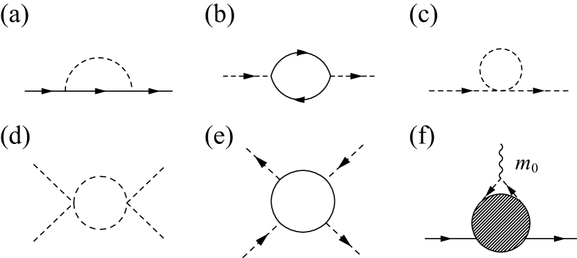
Figure 5: (a-e) One-loop Feynman diagrams included in the renormalized perturbation analysis. (f) $\Gamma^{(2,2)}(k,k;q,q)$. The solid/broken line is fermion/boson line respectively. A wavy line represents a boson mass $m_{0}$, that comes with a pair of boson lines.

In terms of the renormalized perturbation theory, the renormalization conditions shall be satisfied perturbatively in the Yukawa coupling $g$ and the $\phi^{4}$ coupling $\lambda$. To this end, we treat as perturbations $g$ and $\lambda$ in $S_{E}$ as well as the counterterms $S_{c}$ and treat the quadratic part in $S_{E}$ as the free part. Eq. (103) shows that for fixed $N_{F}$ and $N_{B}$, the number of the internal integral variables ($L$) increases with a unit of $g^{2}$ or $\lambda$. We thus treat $g^{2}$ and $\lambda$ as the same order of the smallness in the perturbation analysis. The standard Dyson-Feynman perturbation theory leads to following one-loop terms ($L=1$) for the amputated 1PI connected Green’s functions (Fig. 5(a-e)),

$$\overline{G}^{-1}_{\pm}(k)=\overline{G}^{-1}_{\pm,0}(k)+(\delta_{\pm}i\omega\mp\delta v_{\pm}\!\ l)$$

$$\hskip 14.22636pt-g^{2}\int_{q}\overline{G}_{\mp,0}(k+q)\overline{G}_{\phi,0}(q)+{\cal O}(g^{4},g^{2}\lambda,\lambda^{2}),$$ (126)

$$\overline{G}^{-1}_{\phi}(q)=\overline{G}^{-1}_{\phi,0}(q)+(\delta m^{2}+\delta c^{2}\!\ {\bm{q}}^{2}+\delta_{\phi}\!\ \varepsilon^{2})$$

$$\hskip 5.69046pt+g^{2}\int_{k}\overline{G}_{+,0}(k+q)\overline{G}_{-,0}(k)+\lambda\int_{q^{\prime}}\overline{G}_{\phi,0}(q^{\prime})$$

$$\hskip 28.45274pt+{\cal O}(g^{4},g^{2}\lambda,\lambda^{2}),$$ (127)

$$\overline{\Gamma}_{g}(k,k+q;q)=-g-\delta g+{\cal O}(g^{5},g^{3}\lambda,g\lambda^{2}),$$ (128)

$$\overline{\Gamma}_{\lambda}(q_{1},q_{2},q_{3})=-\lambda-\delta\lambda+\frac{\lambda^{2}}{2}\int_{q}\overline{G}_{\phi,0}(q)\overline{G}_{\phi,0}(q_{1}+q_{2}-q)$$

$$+\lambda^{2}\int_{q}\overline{G}_{\phi,0}(q)\Big{(}\overline{G}_{\phi,0}(q+q_{2}-q_{3})+\overline{G}_{\phi,0}(q+q_{1}-q_{3})\Big{)}$$

$$-g^{4}\int_{k}\overline{G}_{+,0}(k)\overline{G}_{-,0}(k+q_{1})\Big{(}\overline{G}_{+,0}(k+q_{1}-q_{3})$$

$$\hskip 14.22636pt\times\overline{G}_{-,0}(k+q_{1}+q_{2}-q_{3})+\overline{G}_{+,0}(k-q_{2}+q_{3})$$

$$\hskip 19.91684pt\times\overline{G}_{-,0}(k+q_{3})\Big{)}+{\cal O}(\lambda^{3},g^{2}\lambda^{2},g^{4}\lambda,g^{6}),$$ (129)

where renormalized free Green’s functions for fermions and boson are given by

$$\overline{G}^{-1}_{\pm,0}(k)=i\omega\mp v_{\pm}l,\ \ \overline{G}^{-1}_{\phi,0}(q)=m^{2}+c^{2}{\bm{q}}^{2}+\varepsilon^{2}.$$ (130)

The integrals over $q$ or $k$ are defined in Eqs. (94,97,98). All the one-loop terms except for the last term in Eq. (129) have ultraviolet divergences. The last term in Eq. (129) has no influence on the $\beta$ function for $\lambda$; $\beta_{\lambda}(\cdots)$. $\beta_{\lambda}$ within the one-loop level is identical to that in the pure $\phi^{4}$ theory. Note also that $\overline{\Gamma}_{g}(k,k+q;q)$ has no one-loop term beacuse of the Yukawa coupling; $\sigma_{\pm}\sigma_{\pm}\sigma_{\mp}=0$.

IV.3 Calculation of $\int_{q}\overline{G}_{\mp,0}(k+q)\overline{G}_{\phi,0}(q)$ at $d=3$

The 1-loop term in the fermion self-energy (Fig. 5(a)) has no linear divergence in $\Lambda$, while it has the logarithmic divergence in large $\Lambda$. To see this, we take $\overline{\Lambda}_{B}$ to the infinite in Eq. (97) and see how the integral depends on the UV cutoff for the boson momentum, $\Lambda_{B}$. Carry out first an integral over an angle between the internal boson momentum and external fermion momentum,

$$\int_{q}\overline{G}_{+,0}(k+q)\overline{G}_{\phi,0}(q)=\frac{1}{8\pi^{3}}\int^{\infty}_{-\infty}d\varepsilon\int^{\Lambda_{B}}_{0}Q^{2}dQ$$

$$\hskip 22.76228pt\times\int^{1}_{-1}dt\!\ \frac{1}{\varepsilon^{2}+c^{2}Q^{2}+m^{2}}\frac{1}{i\omega-v_{+}l+i\varepsilon-v_{+}Qt}$$

$$\ \ \ =-\frac{1}{8\pi^{3}v_{+}}\int^{\Lambda_{B}}_{0}QdQ$$

$$\int^{\infty}_{-\infty}\frac{d\varepsilon}{(\varepsilon+iM)(\varepsilon-iM)}\!\ {\rm Log}\!\ \Big{[}\frac{i\omega+i\varepsilon-v_{+}l-v_{+}Q}{i\omega+i\varepsilon-v_{+}l+v_{+}Q}\Big{]},$$ (131)

with $q\equiv(i\varepsilon,{\bm{q}})$, $k\equiv(i\omega,{\bm{k}})$, ${\bm{k}}=(k_{F}+l)\hat{\Omega}$, $|{\bm{q}}|\equiv Q$, $Qt\equiv{\bm{q}}\cdot\hat{\Omega}$ and $M^{2}\equiv c^{2}Q^{2}+m^{2}$. The integral is odd under $(\omega,l)\rightarrow-(\omega,l)$. Thus, without loss of generality, we can assume that $l$ is positive. In the complex variable plane of $\varepsilon$, the integrand in the right hand side has a branch cut of the logarithmic function, which runs from $\varepsilon=-\omega-i\!\ v_{+}(l+Q)$ to $\varepsilon=-\omega-iv_{+}(l-Q)$. For $(0<)Q<l$, the integral can be given by a pole contribution at $\varepsilon=\pm iM$. For $l<Q$, The real axis of $\varepsilon$ crosses the branch cut, so that the integral is composed of the pole contribution and an integral along the branch cut from $\varepsilon=-\omega$ to $\varepsilon=-\omega-i\!\ v_{+}(l\pm Q)$ respectively. This leads to

$$\int_{q}\overline{G}_{+,0}(k+q)\overline{G}_{\phi,0}(q)=-\frac{1}{8\pi^{2}v_{+}}$$

$$\Bigg{(}\int^{l}_{0}dQ\!\ \frac{Q}{M}\!\ {\rm Log}\Big{[}\frac{i\omega-M-v_{+}l-v_{+}Q}{i\omega-M-v_{+}l+v_{+}Q}\Big{]}+\int^{\Lambda_{B}}_{l}dQ\!\ \frac{Q}{M}$$

$$\ \ \bigg{\{}{\rm Log}\Big{[}\frac{M+v{+}l+v_{+}Q-i\omega}{M-v_{+}l+v_{+}Q+i\omega}\Big{]}+{\rm Log}\Big{[}\frac{M+i\omega}{M-i\omega}\Big{]}\bigg{\}}\Bigg{)},$$ (132)

for $l>0$. At the massless point $(m=0)$, the integral over $Q$ can be further carried out explicitly. Besides, replacing $v_{+}$ by $-v_{-}$ in Eq. (131) is equivalent to changing $\omega$ by $-\omega$ and adding the overall minus sign in Eq. (131). This leads to

$$\int_{q}\overline{G}_{\sigma,0}(k+q)\overline{G}_{\phi,0}(q)\Big{|}_{m=0}= -\frac{\sigma}{8\pi^{2}cv_{\sigma}}\bigg{\{}-\Big{(}\frac{1}{c+v_{\sigma}}-\frac{1}{c-v_{\sigma}}\Big{)}(v_{\sigma}l-i\sigma\omega)\!\ {\rm Log}(v_{\sigma}l-i\sigma\omega)$$

$$+\Big{(}\frac{1}{c+v_{\sigma}}-\frac{1}{c}\Big{)}(cl+i\sigma\omega)\!\ {\rm Log}(cl+i\sigma\omega)-\Big{(}\frac{1}{c-v_{\sigma}}-\frac{1}{c}\Big{)}(cl-i\sigma\omega)\!\ {\rm Log}(cl-i\sigma\omega)$$

$$-2\!\ \frac{i\sigma\omega-v_{\sigma}l}{c+v_{\sigma}}\!\ \log\big{(}(c+v_{\sigma})\Lambda_{B}\big{)}+2\!\ \frac{i\sigma\omega}{c}\!\ \log\big{(}c\Lambda_{B}\big{)}-2\!\ \frac{i\sigma\omega-v_{\sigma}l}{c+v_{\sigma}}+2\!\ \frac{i\sigma\omega}{c}+{\cal O}(\omega/\Lambda_{B},l/\Lambda_{B})\bigg{\}},$$ (133)

with $\sigma=\pm$. When substituted into Eq. (126) in favor for $\overline{G}^{-1}_{\pm}(k)$, Eq. (133) leads to the UV logarithmic divergence in the linear coefficients of the frequency $\omega$ and the one-dimensional momentum $l$;

$$\overline{G}^{-1}_{\pm}(k)= \overline{G}^{-1}_{\pm,0}(k)+(\delta_{\pm}i\omega\mp\delta v_{\pm}l)$$

$$\ \ +(\ldots)\!\ \ln\Lambda\!\ i\omega+(\ldots)\!\ \ln\Lambda\!\ l+\cdots.$$ (134)

Eq. (133) also has the weak IR singularity ($\omega\ln\omega$ type; omitted as ‘$\cdots$’ in Eq. (134)). When being taken derivatives of with respect to $\omega$ or $l$, the weak IR singularity leads to the IR logarithmic singularity. The IR logarithmic singularity is controlled by the finite RG scale $\kappa$ in the RG conditions; Eq. (123) with $\omega$ or $v_{\pm}l=\kappa$. Thereby, $\ln\kappa$ comes in pairs with $\ln\Lambda$,

$$\overline{G}^{-1}_{\pm}(\omega=l=0)=\overline{G}^{-1}_{\pm,0}(\omega=l=0)=0,$$

$$\frac{\partial\overline{G}^{-1}_{\pm}(\omega,l)}{\partial(i\omega)}\Big{|}_{v_{\pm}l=0,\omega=\kappa}=1+\delta_{\pm}+(\cdots)\ln\bigg{(}\frac{\Lambda}{\kappa}\bigg{)}+\cdots,$$

$$\frac{\partial\overline{G}^{-1}_{\pm}(\omega,l)}{\partial(\mp v_{\pm}l)}\Big{|}_{v_{\pm}l=\kappa,\omega=0}=1+\frac{\delta v_{\pm}}{v_{\pm}}+(\cdots)\ln\bigg{(}\frac{\Lambda}{\kappa}\bigg{)}+\cdots.$$

IV.4 Calculation of $\int_{k}\overline{G}_{+,0}(k+q)\overline{G}_{-,0}(k)$ and $\int_{q}\overline{G}_{\phi,0}(q)$ at $d=3$

The 1-loop terms in the boson self-energy have two contributions (Fig. 5(b,c)). One with an integral over internal boson loop (Fig. 5(c)), and the other with an integral over internal fermion loop (Fig. 5(b)). The integral over the boson loop does not depend on external momentum and frequency,

$$\int_{q}\overline{G}_{\phi,0}(q) =\frac{1}{c^{3}}\int^{+\infty}_{-\infty}\frac{d\varepsilon}{2\pi}\int_{|{\bm{q}}|<\Lambda_{B}}\frac{d{\bm{q}}}{(2\pi)^{3}}\frac{1}{\varepsilon^{2}+c^{2}{\bm{q}}^{2}+m^{2}}$$

$$\rightarrow\frac{\Lambda^{2}_{B}}{16\pi^{2}c^{3}}\ \ \!\ (m\rightarrow 0).$$ (135)

The integral over the fermion loop has the logarithmic divergence in the ultraviolet cutoff. To see this UV divergence, integrate first an angle between the internal fermion momentum and external boson momentum, $\theta$,

$$\int_{k}\overline{G}_{+,0}(k+q)\overline{G}_{-,0}(k)=k^{2}_{F}\int\frac{d^{2}\hat{\Omega}}{(2\pi)^{2}}$$

$$\!\ \int^{+\Lambda_{F}}_{-\Lambda_{F}}\frac{dl}{2\pi}\int^{\overline{\Lambda}_{F}}_{-\overline{\Lambda}_{F}}\frac{d\omega}{2\pi}\frac{1}{i\omega-v_{+}l}\frac{1}{i(\omega+\varepsilon)+v_{-}(l+m)}$$

$$=\frac{1}{2\pi}\frac{k^{2}_{F}}{v_{-}q}\int^{+\Lambda_{F}}_{-\Lambda_{F}}\frac{dl}{2\pi}\int^{\overline{\Lambda}_{F}}_{-\overline{\Lambda}_{F}}\frac{d\omega}{2\pi}$$

$$\hskip 45.52458pt\frac{1}{i\omega-v_{+}l}\!\ {\rm Log}\bigg{[}\frac{i(\omega+\varepsilon)+v_{-}l+v_{-}q}{i(\omega+\varepsilon)+v_{-}l-v_{-}q}\bigg{]},$$ (136)

where $k\equiv(\omega,{\bm{k}})$, ${\bm{k}}\equiv(k_{F}+l)\hat{\Omega}$, $q\equiv(\varepsilon,{\bm{q}})$, and ${\bm{q}}\cdot\hat{\Omega}=q\cos\theta=m$ (Henceforth we will often write $|{\bm{q}}|$ as $q$, as far as the scalar $|{\bm{q}}|$ can be obviously distinguishable from the four-dimensional $q=(\varepsilon,{\bm{q}})$). For simplicity, we consider the case with $v_{+}=v_{-}=v$, while putting only the result for the general case ($v_{+}\neq v_{-}$) in Eq. (139). By choosing $v\Lambda_{F}=\overline{\Lambda}_{F}$, we introduce $Q/z\equiv\omega+ivl$ with $Q^{2}\equiv\omega^{2}+(vl)^{2}$;

$$\int_{k}\overline{G}_{+,0}(k+q)\overline{G}_{-,0}(k)\Big{|}_{v_{+}=v_{-}=v}=-\frac{1}{2\pi}\frac{k^{2}_{F}}{v^{2}q}$$

$$\ \ \times\int^{\overline{\Lambda}_{F}}_{0}\frac{dQ}{2\pi}\oint_{|z|=1}\frac{dz}{2\pi}\!\ {\rm Log}\bigg{[}\frac{iz+(i\varepsilon+vq)/Q}{iz+(i\varepsilon-vq)/Q}\bigg{]}.$$ (137)

As a function of the complex variable $z$, the integrand in the right hand side has a branch cut from $z=-\xi\equiv-(\varepsilon+ivq)/Q$ to $z=-\xi^{*}\equiv-(\varepsilon-ivq)/Q$. For $Q<\varepsilon$, the $z$-integral along the unit circle is contractible. For $\varepsilon<Q<R\equiv\sqrt{\varepsilon^{2}+(vq)^{2}}$, the $z$-integral along the unit circle is contracted into an integral along a part of the branch cut. Thereby, the integral runs along one side and the other side of a line, that runs from $z=z_{0}\equiv-\varepsilon/Q+i\sqrt{1-(\varepsilon/Q)^{2}}$ to $z=z^{*}_{0}$ with $|z_{0}|=1$. For $R<Q$, the $z$-integral along the unit circle can be contracted into an integral along a loop, that goes around the whole branch cut. That says, the integral reduces to

$$\int_{k}\overline{G}_{+,0}(k+q)\overline{G}_{-,0}(k)\Big{|}_{v_{+}=v_{-}=v}$$

$$=\frac{i}{4\pi^{2}}\frac{k^{2}_{F}}{v^{2}q}\Bigg{(}\int^{\overline{\Lambda}_{F}}_{R}dQ(-\xi^{*}+\xi)+\int^{R}_{\varepsilon}dQ(z_{0}-z^{*}_{0})\Bigg{)}$$

$$=-\frac{k^{2}_{F}}{2\pi^{2}v}\bigg{\{}\log\Big{(}\frac{\overline{\Lambda}_{F}}{R}\Big{)}+1-\frac{\varepsilon}{vq}{\rm ArcTan}\big{(}\frac{vq}{\varepsilon}\Big{)}\bigg{\}}.$$ (138)

In the general case of $v_{+}\neq v_{-}$, Eq. (136) can be similarly evaluated. The result is

$$\int_{k}\overline{G}_{+,0}(k+q)\overline{G}_{-,0}(k)=$$

$$\ \ \ -\frac{k^{2}_{F}}{\pi^{2}(v_{+}+v_{-})}\Bigg{\{}\log\bigg{(}\frac{\overline{\Lambda}_{F}}{R}\bigg{)}+1-\frac{\varepsilon}{v_{-}q}\frac{(v_{+}+v_{-})}{2v_{+}}{\rm ArcTan}\Big{[}\frac{v_{-}q}{\varepsilon}\Big{]}-\frac{\varepsilon}{2v_{+}q}{\rm ArcTan}\bigg{[}\frac{(v_{+}-v_{-})\sin 2\theta}{(v_{+}+v_{-})-(v_{+}-v_{-})\cos 2\theta}\bigg{]}$$

$$\ \ \ \ -\frac{1}{4}\log\bigg{[}\frac{(v_{+}+v_{-})^{2}+(v_{+}-v_{-})^{2}-2(v_{+}+v_{-})(v_{+}-v_{-})\cos 2\theta}{(v_{+}+v_{-})^{2}}\bigg{]}\Bigg{\}}+{\cal O}(q/\Lambda_{F}),$$ (139)

with $\overline{\Lambda}_{F}\equiv v_{-}\Lambda_{F}$, $R^{2}\equiv\varepsilon^{2}+v^{2}_{-}q^{2}$ and $(\cos\theta,\sin\theta)\equiv(\varepsilon,v_{-}q)/R$. In Eq. (127) in favor for $\overline{G}^{-1}_{\phi}(q)$, Eqs. (138,139) bring the UV logarithmic divergence into the boson mass. The UV divergence comes with the IR logarithmic divergence;

$$\overline{G}^{-1}_{\phi}(q)= \overline{G}^{-1}_{\phi,0}(q)+(\delta m^{2}+\delta c^{2}q^{2}+\delta_{\phi}\varepsilon^{2})$$

$$\ \ +(\ldots)\!\ k^{2}_{F}\!\ \log\Big{(}\frac{\Lambda}{R}\Big{)}+\cdots,$$

with $R^{2}\equiv\varepsilon^{2}+(v{\bm{q}})^{2}$. The IR divergence is controlled by the RG scale variable $\kappa$ in Eq. (123), where $R$ is replaced by $\kappa$.

IV.5 Calculation of the boson and fermion integrals in Eq. (129) at $d=3$

The 1-loop term in the four-point boson vertex function has two contributions (Fig. 5(d,e)). The 1-loop term with the internal fermion integral has the IR quadratic divergence (Fig. 5(e)). To see this, set only the external boson frequencies to be finite, $q_{i}=(p_{i},{\bm{0}})$, and integrate over the fermion frequency $\omega$,

$$\int_{k}\overline{G}_{+,0}(k)\overline{G}_{-,0}(k+q_{1})$$

$$\hskip 28.45274pt\times\overline{G}_{+,0}(k+q_{1}-q_{3})\overline{G}_{-,0}(k+q_{1}+q_{2}-q_{3})$$

$$=-i\frac{k^{2}_{F}}{\pi(v_{+}+v_{-})}\int^{+\infty}_{-\infty}\frac{dX}{2\pi}\Big{\{}\frac{1}{X+ip_{1}}\frac{1}{X+ip_{3}}\frac{1}{p_{2}-p_{3}}$$

$$\hskip 71.13188pt+\frac{1}{X+ip_{2}}\frac{1}{X+ip_{4}}\frac{1}{-p_{2}+p_{3}}\Big{\}}$$ (140)

with $k\equiv(\omega,{\bm{k}})$, ${\bm{k}}\equiv(k_{F}+l)\hat{\Omega}$ and $X\equiv(v_{+}+v_{-})l$. Here $p_{1}$, $p_{2}$, $p_{3}$, $p_{4}=p_{1}+p_{2}-p_{3}$ are external boson frequencies of $q_{1}$, $q_{2}$, $q_{3}$ and $q_{4}$ respectively. When these frequencies are chosen with either ${\rm sgn}(p_{1}p_{3})<0$ or ${\rm sgn}(p_{2}p_{4})<0$, the integral over the one-dimensional fermion momentum $l\equiv X/(v_{+}+v_{-})$ gives a quadratic divergent term in the small external frequencies. When these frequencies are chosen with ${\rm sgn}(p_{1}p_{3})>0$ and ${\rm sgn}(p_{2}p_{4})>0$ as in Eq. (124), the integral over $X$ leads to zero.

The 1-loop term with the internal boson integral has the UV logarithmic divergence (Fig. 5(d)). In the massless case ($m=0$), the UV divergence comes with an IR logarithmic divergence. The IR divergence can be controlled by choosing the external boson frequencies as in Eqs. (124,125). Thereby, the external boson frequencies play role of the RG scale variable $\kappa$,

$$\int_{q}\overline{G}_{\phi,0}(q)\overline{G}_{\phi,0}(q_{1}+q_{2}-q)$$

$$=\int^{+\infty}_{-\infty}\frac{d\varepsilon}{2\pi}\int_{|{\bm{q}}|<\Lambda_{B}}\frac{d^{3}{\bm{q}}}{(2\pi)^{3}}\frac{1}{\varepsilon^{2}+c^{2}{\bm{q}}^{2}}\frac{1}{(\varepsilon-y)^{2}+c^{2}{\bm{q}}^{2}}$$

$$=\frac{\log\big{(}\frac{2c\Lambda_{B}}{y}\big{)}}{8\pi^{2}c^{3}}+{\cal O}(\Lambda^{-2}_{B}).$$ (141)

Here $y=4\kappa/3$ for the first term in Eq. (129) (particle-particle channel) and $y=\kappa/3$ for the other two in Eq. (129) (particle-hole channel). When substituted into Eq. (129) in favor for $\overline{\Gamma}_{\lambda}$, Eq. (141) leads to the UV logarithmic divergence in the $\phi^{4}$ coupling,

$$\overline{\Gamma}_{\lambda}(q_{1},q_{2},q_{3})\Big{|}_{q_{1}=(\kappa,0),q_{2}=(\kappa/3,0),q_{3}=(2\kappa/3,0)}$$

$$\ \ \ =-\lambda-\delta\lambda+(\ldots)\!\ \log\Big{(}\frac{\Lambda}{\kappa}\Big{)}+\cdots.$$

IV.6 determination of the counterterms and $\beta$ functions

By substituting Eqs. (133,135,139,141) into Eqs. (126,127,129) and imposing the conditions Eq. (123) on the renormalized vertex functions, we determine the counterterms in $S_{c}$; $\delta m^{2}$, $\delta c^{2}$, $\delta_{\phi}$, $\delta_{\pm}$, $\delta v_{\pm}$, $\delta g$ and $\delta\lambda$. The counterterms are given as functions of the renormalized physical quantities, $m^{2}$, $c^{2}$, $v_{\pm}$, $g$, $\lambda$, the RG scale $\kappa$, the Fermi wavelength $k_{F}$ and the UV cutoff $\Lambda$. So are the bare quantities, $m^{2}_{0}$, $c^{2}_{0}$, $v_{\pm 0}$, $g_{0}$, $\lambda_{0}$, and the renormalization of the field operator amplitudes, $Z_{\phi}$ and $Z_{\pm}$;

$$\left\{\begin{array}[]{c}m^{2}_{0}=M^{2}_{0}(m^{2},c^{2},v_{+},v_{-},g,\lambda,\kappa,k_{F},\Lambda),\\ c^{2}_{0}=C^{2}_{0}(m^{2},c^{2},\cdots,g,\lambda,\kappa,k_{F},\Lambda),\\ v_{\sigma 0}=V_{\sigma 0}(m^{2},c^{2},\cdots,g,\lambda,\kappa,k_{F},\Lambda),\\ g_{0}=G_{0}(m^{2},c^{2},\cdots,g,\lambda,\kappa,k_{F},\Lambda),\\ \lambda_{0}=\Lambda_{0}(m^{2},c^{2},\cdots,g,\lambda,\kappa,k_{F},\Lambda),\\ \end{array}\right.$$ (147)

and

$$\left\{\begin{array}[]{c}Z_{\phi}=Z_{\phi}(m^{2},c^{2},v_{+},v_{-},g,\lambda,\kappa,k_{F},\Lambda),\\ Z_{\sigma}=Z_{\sigma}(m^{2},c^{2},\cdots,g,\lambda,\kappa,k_{F},\Lambda),\\ \end{array}\right.$$ (150)

with $\sigma=\pm$. Eqs. (147,150) define a relation between bare quantities and renormalized physical quantities, in which all the universal information of the quantum criticality are encoded. To decode the information of the criticality, Eq. (118) and their derivative with respect to the RG scale variable $\kappa$ are used in combination with Eqs. (147,150) (see Sec. VA).

The renormalized perturbation theory determines Eqs. (147,150) perturbatively in $g^{2}$ and $\lambda$. In this work, we shall focus only on the relation at the massless point, and set the renormalized physical mass $m$ to be zero in Eqs. (147,150). Thereby, the first line of Eq. (147) defines a subspace of the quantum critical ‘point’ in a multiple-dimensional parameter space subtended by the bare quantities, $m_{0}$, $c_{0}$, $v_{\sigma 0}$, $g_{0}$, $\lambda_{0}$, and the RG scale variable $\kappa$;

$$m^{2}_{0}=M^{2}_{0}(m^{2}=0,c^{2},v_{+},v_{-},g,\lambda,\kappa,k_{F},\Lambda).$$ (151)

Meanwhile, the other relations in Eqs. (147,150) with $m^{2}=0$ define the critical properties at the quantum critical point;

$$\left\{\begin{array}[]{c}c^{2}_{0}=C^{2}_{0}(m^{2}=0,c^{2},v_{+},v_{-},g,\lambda,\kappa,k_{F},\Lambda),\\ v_{\sigma 0}=V_{\sigma 0}(m^{2}=0,c^{2},\cdots,\lambda,\kappa,k_{F},\Lambda),\\ g_{0}=G_{0}(m^{2}=0,c^{2},\cdots,\lambda,\kappa,k_{F},\Lambda),\\ \lambda_{0}=\Lambda_{0}(m^{2}=0,c^{2},\cdots,\lambda,\kappa,k_{F},\Lambda),\\ Z_{\phi}=Z_{\phi}(m^{2}=0,c^{2},\cdots,\lambda,\kappa,k_{F},\Lambda),\\ Z_{\sigma}=Z_{\sigma}(m^{2}=0,c^{2},\cdots,\lambda,\kappa,k_{F},\Lambda).\\ \end{array}\right.$$ (158)

To be more specific, at the critical point ($m=0$), the counterterms in $S_{c}$ are given as functions of renormalized physical quantities, $\kappa$, $k_{F}$, and $\Lambda$ perturbatively in $g^{2}$ and $\lambda$;

$$\ \ \ \ \delta m^{2}+\delta_{\phi}\kappa^{2}-\frac{g^{2}k^{2}_{F}}{\pi^{2}(v_{+}+v_{-})}\bigg{\{}\log\Big{(}\frac{\overline{\Lambda}_{F}}{\kappa}\Big{)}-\frac{1}{2}\log\Big{(}\frac{2v_{-}}{v_{+}+v_{-}}\Big{)}\bigg{\}}+\frac{\lambda\Lambda^{2}_{B}}{16\pi^{2}c^{3}}=0,$$ (159)

$$\left\{\begin{array}[]{l}\delta_{\sigma}=-\frac{g^{2}}{8\pi^{2}cv_{\overline{\sigma}}}\bigg{\{}\frac{2v_{\overline{\sigma}}}{(c+v_{\overline{\sigma}})c}\log\Big{(}\frac{\Lambda_{B}}{\kappa}\Big{)}-\frac{2}{c+v_{\overline{\sigma}}}\log(c+v_{\overline{\sigma}})+\frac{2}{c}\log c\bigg{\}}\\ \delta v_{\sigma}=-\frac{g^{2}}{8\pi^{2}cv_{\overline{\sigma}}}\bigg{\{}\frac{2v_{\overline{\sigma}}}{c+v_{\overline{\sigma}}}\log\Big{(}\frac{v_{\sigma}\Lambda_{B}}{\kappa}\Big{)}+\frac{2v_{\overline{\sigma}}}{c+v_{\overline{\sigma}}}\log(c+v_{\overline{\sigma}})-\frac{2v_{\overline{\sigma}}}{c+v_{\overline{\sigma}}}\frac{1}{c-v_{\overline{\sigma}}}(c\log c-v_{\overline{\sigma}}\log v_{\overline{\sigma}})\bigg{\}},\\ \delta\lambda=\frac{\lambda^{2}}{16\pi^{2}c^{3}}\bigg{\{}5\log\Big{(}\frac{3c\Lambda_{B}}{\kappa}\Big{)}+3\log 2\bigg{\}},\ \ \delta_{\phi}=0,\ \ \delta c^{2}=0,\ \ \delta g=0.\\ \end{array}\right.$$ (163)

with $\overline{\sigma}=\mp$ for $\sigma=\pm$. Here the followings were used from Eq. (139),

$$\frac{\partial}{\partial\varepsilon}\bigg{(}\int_{k}\overline{G}_{+,0}(k+q)\overline{G}_{-,0}(k)\bigg{)}\Big{|}_{\varepsilon=\kappa,{\bm{q}}=0}=\frac{\partial}{\partial(c|{\bm{q}}|)}\bigg{(}\int_{k}\overline{G}_{+,0}(k+q)\overline{G}_{-,0}(k)\bigg{)}\Big{|}_{\varepsilon=0,c|{\bm{q}}|=\kappa}=\frac{k^{2}_{F}}{\pi^{2}(v_{+}+v_{-})\kappa}.$$ (164)

When substituted in Eqs. (127,123), Eq. (164) cancels the first order term in $k^{2}_{F}$ in the right hand side of the conditions for the boson self energy in Eq. (123).

In terms of Eqs. (163,159) and $m=0$, a set of the bare physical quantities, $m_{0}$, $c_{0}$, $v_{\sigma 0}$, $g_{0}$, $\lambda_{0}$, are given as functions of renormalized physical quantities, the RG scale variable $\kappa$, the Fermi wavelength $k_{F}$ and the UV cutoff $\Lambda$,

$$m^{2}_{0} =Z^{-1}_{\phi}(m^{2}+\delta m^{2})=\delta m^{2}=-\frac{\lambda\Lambda^{2}_{B}}{16\pi^{2}c^{3}}$$

$$+\frac{g^{2}k^{2}_{F}}{\pi^{2}(v_{+}+v_{-})}\bigg{\{}\log\Big{(}\frac{\overline{\Lambda}_{F}}{\kappa}\Big{)}-\frac{1}{2}\log\Big{(}\frac{2v_{-}}{v_{+}+v_{-}}\Big{)}\bigg{\}}+\cdots$$ (165)

$$v_{\sigma 0} =Z^{-1}_{\sigma}(v_{\sigma}+\delta v_{\sigma})=v_{\sigma}-\delta_{\sigma}v_{\sigma}+\delta v_{\sigma}+\cdots,$$ (166)

$$c^{2}_{0} =c^{2}+\cdots,\ \ \ \ \lambda_{0}=\lambda+\delta\lambda,$$ (167)

$$g_{0} =(1-\frac{1}{2}\delta_{\phi})(1-\frac{1}{2}\delta_{+})(1-\frac{1}{2}\delta_{-})g$$

$$=(1-\frac{1}{2}\delta_{+}-\frac{1}{2}\delta_{-})g+\cdots,$$ (168)

with $\sigma=\pm$. Here $\delta_{\sigma}$, $\delta v_{\sigma}$, $\delta\lambda$ in the right hand sides are given in Eq. (163).‘$\cdots$’ in the right hand sides stands for the higher-order contributions in $g^{2}$ and $\lambda$. By inverse solutions of Eqs. (166,167,168,163), $c$, $v_{\pm}$, $g$, $\lambda$ are given as functions of $c_{0}$, $v_{\pm 0}$, $g_{0}$, $\lambda_{0}$, $\kappa$, $k_{F}$ and $\Lambda$. On substitution of such solutions into Eq. (165), $m_{0}$ is given as a function of $c_{0}$, $v_{\pm 0}$, $g_{0}$, $\lambda_{0}$, $\kappa$, $k_{F}$ and $\Lambda$. Such a function for $m_{0}$ defines a subspace of $m=0$ in a multiple-dimensional parameter space subtended by the bare physical quantities and the RG scale variable $\kappa$. The subspace of $m=0$ defines the quantum critical ‘point’ in the parameter space of the bare quantities and $\kappa$.

Let us introduce a derivative with respect to the RG scale $\kappa$ within the subspace of $m=0$ and with fixed values of the other bare quantities, $k_{F}$ and the UV cutoff;

$$\frac{\partial}{\partial\ln\kappa}\Big{|}_{c_{0},v_{\pm 0},g_{0},\lambda_{0},k_{F},\Lambda:{\rm fixed}}\equiv\frac{\partial}{\partial\ln\kappa}\Big{|}_{\cdots}.$$ (169)

The following identities hold true trivially;

$$\frac{\partial c_{0}}{\partial\ln\kappa}\Big{|}_{\cdots}=\frac{\partial v_{\sigma 0}}{\partial\ln\kappa}\Big{|}_{\cdots}=\frac{\partial g_{0}}{\partial\ln\kappa}\Big{|}_{\cdots}=\frac{\partial\lambda_{0}}{\partial\ln\kappa}\Big{|}_{\cdots}=0,$$ (170)

with $\sigma=\pm$. On application of such $\ln\kappa$-derivative onto Eqs. (166,167,168) with Eq. (170) in their left hand sides, $\beta$ functions of the physical quantities are obtained as their $\ln\kappa$-derivatives. The $\beta$ functions are calculated perturbatively in the Yukawa coupling $g^{2}$ and the $\phi^{4}$ coupling $\lambda$,

$$\frac{\partial v_{\sigma}}{\partial\ln\kappa}\Big{|}_{\cdots}=\frac{\partial\delta_{\sigma}}{\partial\ln\kappa}v_{\sigma}-\frac{\partial\delta v_{\sigma}}{\partial\ln\kappa}+{\cal O}(g^{4},g^{2}\lambda,\lambda^{2})$$

$$=\frac{g^{2}}{4\pi^{2}c(c+v_{\overline{\sigma}})}\Big{(}\frac{v_{\sigma}}{c}-1\Big{)}+\cdots\equiv\beta_{v_{\sigma}}(c,\cdots),$$ (171)

$$\frac{\partial c}{\partial\ln\kappa}\Big{|}_{\cdots}=0+\cdots\equiv\beta_{c}(c,\cdots),$$ (172)

$$\frac{\partial g}{\partial\ln\kappa}\Big{|}_{\cdots}=\frac{g}{2}\Big{(}\frac{\partial\delta_{+}}{\partial\ln\kappa}+\frac{\partial\delta_{-}}{\partial\ln\kappa}\Big{)}+{\cal O}(g^{5},g^{3}\lambda,g\lambda^{2})$$

$$=\frac{g^{3}}{8\pi^{2}c^{2}}\Big{(}\frac{1}{c+v_{+}}+\frac{1}{c+v_{-}}\Big{)}+\cdots\equiv\beta_{g}(c,\cdots),$$ (173)

$$\frac{\partial\lambda}{\partial\ln\kappa}\Big{|}_{\cdots}=\frac{5\lambda^{2}}{16\pi^{2}c^{3}}+{\cal O}(\lambda^{3},\lambda^{2}g^{2},\lambda g^{4},g^{6})\equiv\beta_{\lambda}(c,\cdots),$$ (174)

with $\sigma=\pm$ and $\overline{\sigma}=\mp$. Here ‘$\cdots$’ in the right hand side refers to the higher-order terms in $g^{2}$ and $\lambda$. Importantly, the $\beta$ functions are given only by the renormalized physical quantities themselves.

The leading-order $\beta$ functions of $g$ as well as $\lambda$ dictate that in the low-energy limit ($\ln\kappa\rightarrow-\infty$), the Yukawa coupling $g$ and $\phi^{4}$ coupling $\lambda$ are renormalized into the zero. The marginal irrelevance of $g$ and $\lambda$ in the IR limit justifies a posteriori the perturbative calculation in small $g^{2}$ and $\lambda$. The $\beta$ functions of the two Fermi velocities shows that in the IR limit, both $v_{+}$ and $v_{-}$ are renormalized into the same critical velocity as the boson velocity $c$. Within the one-loop level, the boson velocity has no renormalization; $\beta_{c}=0$.

V Callan-Symanzik equation and its approximate solution

The $\beta$ functions appear in the Callan-Symanzik (CS) equations for the renormalized Green’s functions. The role of the $\beta$ functions become clear, when the CS equations are solved in favor for the Green’s functions Peskin and Schroeder (1995); Amit and Martin-Mayor (2005). In this section, the CS equation for the two-point fermion Green’s functions will be derived first. In the latter part of this section, the CS equations are solved in favor for the renormalized fermion Green’s functions.

V.1 derivation of Callan-Symanzik equation at QCP

Let us begin with the relation between the renormalized two-point fermion Green’s function and the bare one. From Eq. (118), the relation is,

$$Z_{\sigma}(m^{2}=0,c^{2},v_{+},v_{-},g,\lambda,\kappa,\Lambda)$$

$$\ \ \ \ \ \times\overline{G}_{\sigma}(k;m^{2}=0,c^{2},v_{+},v_{-},g,\lambda,\kappa)$$

$$\ \ \ \hskip 42.67912pt=G_{\sigma}(k;m^{2}_{0},c^{2}_{0},v_{+0},v_{-0},g_{0},\lambda_{0},\Lambda).$$ (175)

Here the $k_{F}$-dependence was trivially omitted, and will be omitted henceforth unless dictated otherwise. In Eq. (175), $Z_{\sigma}$ and $\overline{G}_{\sigma}$ in the left hand sides are given as functions of the renormalized physical quantities, $c$, $v_{\pm}$, $g$, $\lambda$, the RG scale variable $\kappa$ and the UV cutoff $\Lambda$. By Eqs. (166,167,168,163), such renormalized physical quantities are given as functions of $c_{0}$, $v_{\pm 0}$, $g_{0}$, $\lambda_{0}$, the RG scale variable $\kappa$, and $\Lambda$. $G_{\sigma}$ in the right hand side is originally given as a function of $m_{0}$, $c_{0}$, $v_{\pm 0}$, $g_{0}$, $\lambda_{0}$ and the UV cutoff $\Lambda$. By Eq. (165) with Eqs. (166,167,168,163), $m_{0}$ is given by $c_{0}$, $v_{\pm 0}$, $g_{0}$, $\lambda_{0}$, the RG scale variable $\kappa$, and $\Lambda$. With this in mind, take the $\kappa$-derivative of Eq. (175) with respect to Eq. (169). The derivative gives the following inhomogeneous CS equation

$$\Big{\{}\frac{\partial}{\partial\ln\kappa}+\beta_{c}\frac{\partial}{\partial c}+\sum_{\sigma^{\prime}=\pm}\beta_{v_{\sigma^{\prime}}}\frac{\partial}{\partial v_{\sigma^{\prime}}}+\beta_{g}\frac{\partial}{\partial g}+\beta_{\lambda}\frac{\partial}{\partial\lambda}$$

$$\ \ +\gamma_{\sigma}\Big{\}}\overline{G}_{\sigma}(k;m^{2}=0,c^{2},\cdots,\lambda,\kappa)=\frac{\partial m^{2}_{0}}{\partial\ln\kappa}\frac{\partial G_{\sigma}}{\partial m^{2}_{0}}.$$ (176)

Here $\gamma_{\sigma}$ ($\sigma=\pm$) is called as $\gamma$ function and it is given by the $\kappa$-derivative of the renormalizations of the field operator amplitudes,

$$\frac{\partial\ln Z_{\sigma}}{\partial\ln\kappa}\Big{|}_{\cdots} =\frac{\partial\ln(1+\delta_{\sigma})}{\partial\ln\kappa}\Big{|}_{\cdots}$$

$$=\frac{g^{2}}{4\pi^{2}c^{2}(c+v_{\overline{\sigma}})}+{\cal O}(g^{4},g^{2}\lambda,\lambda^{2})\equiv\gamma_{\sigma}.$$ (177)

with $\sigma=\pm$ and $\overline{\sigma}=\mp$.

Note that the right hand side of Eq. (176) is at most on the order of ${\cal O}(g^{4})$ and negligible within the one-loop level calculation. Namely, Eq. (165) leads to

$$\frac{\partial m^{2}_{0}}{\partial\ln\kappa}\Big{|}_{\cdots}=-\frac{g^{2}k^{2}_{F}}{\pi^{2}(v_{+}+v_{-})}+{\cal O}(g^{4},g^{2}\lambda,\lambda^{2}).$$ (178)

The partial derivative of the bare fermion Green’s function with respect to the bare boson mass results in an amputated 1PI connected Green’s function with two boson lines and two fermion lines. Such is at most on the order of ${\cal O}(g^{2})$ too;

$$\frac{\partial G_{\sigma}(k)}{\partial m^{2}_{0}}=G_{\sigma}(k)\frac{\partial G^{-1}_{\sigma}(k)}{\partial m^{2}_{0}}G_{\sigma}(k)$$

$$\ \ \ \equiv\int_{q}G_{\sigma}(k)\Gamma^{(2,2)}_{\sigma}(k,k;q,q)G_{\sigma}(k)={\cal O}(g^{2}).$$ (179)

Here $\Gamma^{(2,2)}_{\sigma}(k,k;q,q)$ is the amputated 1PI connected Green’s function with two external bosons and two external fermions lines (Fig. 5(f)). From Eqs. (178,179), the right hand side of Eq. (176) can be neglected within the one-loop order;

$$\Big{\{}\frac{\partial}{\partial\ln\kappa}+\sum_{\sigma^{\prime}=\pm}\beta_{v_{\sigma^{\prime}}}\frac{\partial}{\partial v_{\sigma^{\prime}}}+\beta_{g}\frac{\partial}{\partial g}$$

$$\hskip 8.5359pt+\gamma_{\sigma}\Big{\}}\overline{G}_{\sigma}(l,\omega;m^{2}=0,c^{2},\cdots,\kappa)={\cal O}(g^{4},g^{2}\lambda,\lambda^{2}),$$ (180)

with $k\equiv({\bm{k}},\omega)$ and ${\bm{k}}\equiv(k_{F}+l)\Omega$. Here those terms with $\partial_{c}$ and $\partial_{\lambda}$ are omitted from the left hand side in Eq. (176), because $\beta_{c}=0$ at the one-loop level, and the $\lambda$-dependence of $\overline{G}_{\sigma}$ starts from ${\cal O}(g^{2}\lambda)$, which gives out ${\cal O}(g^{2}\lambda^{2})$ in the right hand side of Eq. (180). In the next section, we shall solve this homogeneous CS equation in favor for the renormalized fermion Green’s functions.

V.2 approximate solutions of Callan-Symanzik equation

The $\beta$ functions for the fermion velocities suggest that the two fermion velocities are renormalized into the boson velocities $c$ in the infrared (IR) limit ($\ln\kappa\rightarrow-\infty$);

$$\frac{dv_{\pm}}{d\ln\kappa}=\frac{g^{2}}{4\pi^{2}c(c+v_{\mp})}\Big{(}\frac{v_{\pm}}{c}-1\Big{)}.$$

That says, at the quantum critical point ($m=0$), the two fermion bands proximate to the Fermi surface have asymptotically the same critical velocity as the boson velocity. We thus assume that $v_{\pm}=c$ in the following analysis. With $v_{\pm}=c$, the CS equation for the fermion Green’s function is given by the homogeneous equation with the one-parameter scaling

$$\Big{\{}\frac{\partial}{\partial\ln\kappa}+\beta_{g}(g)\frac{\partial}{\partial g}+\gamma_{\sigma}(g)\Big{\}}\overline{G}_{\sigma}(l,\omega;g,\kappa)=0.$$ (181)

The $c$ and $v_{\pm}$-dependences of $\overline{G}_{\sigma}$, $\beta_{g}$ and $\gamma_{\sigma}$ can be trivially omitted; $\beta_{v_{\pm}}=\beta_{c}=0$ at $v_{\pm}=c$. From a dimensional analysis, the fermion Green’s function has the following scaling form,

$$\overline{G}_{\sigma}(l,\omega;g,\kappa)=\frac{1}{i\omega-\sigma cl}f_{\sigma}(l/\kappa,\omega/\kappa:g),$$ (182)

with $\sigma=\pm$. Thus, with $\omega=p\sin\theta$ and $cl=p\cos\theta$, the $\kappa$-derivative is replaced by the $p$-derivative with fixed $\theta$;

$$\Big{\{}p\frac{\partial}{\partial p}-\beta_{g}(g)\frac{\partial}{\partial g}+\big{(}1-\gamma_{\sigma}(g)\big{)}\Big{\}}\overline{G}_{\sigma}(p,\theta;g,\kappa)=0.$$ (183)

From Eqs. (173,177), $\beta_{g}$ and $\gamma_{\sigma}$ are given at $v_{\pm}=c$ as;

$$\beta_{g}(g)=\frac{g^{3}}{8\pi^{2}c^{3}},\ \ \ \gamma_{\sigma}(g)=\frac{g^{2}}{8\pi^{2}c^{3}}.$$ (184)

The solution of Eq. (183) is given by

$$\overline{G}_{\sigma}(p,\theta;g,\kappa)=\overline{\cal G}_{\sigma}(\theta;\overline{g}(t;g),\kappa)$$

$$\hskip 56.9055pt\times\exp\bigg{[}\int^{g}_{\overline{g}(t;g)}\frac{1-\gamma_{\sigma}(g^{\prime})}{\beta_{g}(g^{\prime})}dg^{\prime}\bigg{]},$$ (185)

with $t\equiv\ln(p/\kappa)$. $\overline{\cal G}_{\sigma}(\theta;g,\kappa)$ is the Green’s function at $p=\kappa$ ($t=0$);

$$\overline{G}_{\sigma}(p=\kappa,\theta;g,\kappa)\equiv\overline{\cal G}_{\sigma}(\theta;g,\kappa).$$ (186)

$\overline{g}(t;g)$ is a running coupling constant determined by a one-parameter scaling equation with $\beta_{g}$;

$$\frac{\partial\overline{g}(t;g)}{\partial t}=\beta_{g}(\overline{g})=\frac{\overline{g}^{3}}{8\pi^{2}c^{3}},\ \ \overline{g}(t=0;g)=g.$$ (187)

The running coupling constant becomes renormalized into the smaller value in the IR limit,

$$\overline{g}(t;g)=g\sqrt{\frac{1}{1-g^{2}\frac{t}{4\pi^{2}c^{3}}}}.$$ (188)

Namely, for $p\ll\kappa$, $t=\ln(p/\kappa)$ is negative and logarithmically large. $\overline{g}/g$ goes to the zero in the low-energy limit ($p\ll\kappa$). Thus, for smaller $p$ in Eq. (185), $\overline{\cal G}_{\sigma}(\theta;\overline{g},\kappa)$ in its right hand side might be evaluated perturbatively in the small $\overline{g}$. Eq. (126) with $v_{\pm}=c$ gives the second order expression for $\overline{G}_{\sigma}(l,\omega;g,\kappa)$ for small $g$,

$$\overline{G}^{-1}_{\sigma}(l,\omega;g,\kappa) =(i\omega-\sigma cl)$$

$$\ -\frac{g^{2}}{8\pi^{2}c^{3}}(i\omega-\sigma cl)\bigg{\{}\log\Big{[}\frac{\sqrt{(cl)^{2}+\omega^{2}}}{\kappa}\Big{]}-1\bigg{\}},$$ (189)

at $v_{\pm}=c$. Here the following relations are used from Eqs. (133,163),

$$\lim_{v_{\pm}\rightarrow c}\int_{q}\overline{G}_{\sigma}(k+q)\overline{G}_{\phi}(q)\Big{|}_{m=0}$$

$$=-\frac{\sigma}{8\pi^{2}c^{2}}\Bigg{\{}-\frac{1}{2c}(cl+i\sigma\omega)\log\big{(}cl+i\sigma\omega\big{)}$$

$$\hskip 45.52458pt-\frac{1}{2c}(cl+i\sigma\omega)\log\big{(}cl-i\sigma\omega\big{)}+\frac{i\sigma\omega}{c}$$

$$\hskip 56.9055pt-\frac{i\sigma\omega-cl}{c}\log 2+\frac{i\sigma\omega+cl}{c}\log\big{(}c\Lambda_{B}\big{)}\Bigg{\}},$$

$$\lim_{v_{\pm}\rightarrow c}\delta_{\sigma}=-\frac{g^{2}}{8\pi^{2}c^{2}}\bigg{\{}\frac{1}{c}\log\Big{(}\frac{\Lambda_{B}}{\kappa}\Big{)}+\frac{1}{c}\log\Big{(}\frac{c}{2}\Big{)}\bigg{\}},$$

$$\lim_{v_{\pm}\rightarrow c}\delta v_{\sigma}=-\frac{g^{2}}{8\pi^{2}c^{2}}\bigg{\{}\log\Big{(}\frac{c\Lambda_{B}}{\kappa}\Big{)}+\log 2-1\bigg{\}}.$$ (190)

A comparison between Eqs. (186,189) gives

$$\overline{\cal G}^{-1}_{\sigma}(\theta;\overline{g},\kappa)=-\sigma\kappa e^{-\sigma i\theta}\Big{(}1+\frac{\overline{g}^{2}}{8\pi^{2}c^{3}}\Big{)}.$$ (191)

Meanwhile, the exponential factor in Eq. (185) is calculated as

$$\exp\bigg{[}\int^{g}_{\overline{g}(t;g)}\frac{1-\gamma_{\sigma}(g^{\prime})}{\beta_{g}(g^{\prime})}dg^{\prime}\bigg{]}$$

$$=\exp\bigg{[}\int^{0}_{t}dt^{\prime}\bigg{]}\exp\bigg{[}-\int^{g}_{\overline{g}}\frac{1}{g^{\prime}}dg^{\prime}\bigg{]}=\frac{\kappa}{p}\frac{\overline{g}}{g}.$$ (192)

Thus, the renormalized fermion Green’s function near the Fermi surface is obtained as

$$\overline{G}_{\sigma}(l,\omega;g,\kappa) =\frac{1}{i\omega-\sigma cl}\Big{(}1+\frac{\overline{g}^{2}}{8\pi^{2}c^{3}}\Big{)}^{-1}\frac{\overline{g}(t)}{g}$$

$$=\frac{1}{i\omega-\sigma cl}\Big{(}1+\frac{\overline{g}^{2}}{8\pi^{2}c^{3}}\Big{)}^{-1}\sqrt{\frac{1}{1-g^{2}\frac{t}{4\pi^{2}c^{3}}}},$$ (193)

with $t\equiv\ln(\sqrt{(cl)^{2}+\omega^{2}}/\kappa)$. $\overline{g}$ in the right hand side is given by $t$ and $g$ by Eq. (188).

VI Fermionic spectral function and density of states in the quantum critical regime

Previously, the imaginary-time time-ordered fermion Green’s function is obtained as a solution of the Callan-Symanzik equation at the QCP. In this section, we use an analytic continuation ($i\omega\rightarrow\omega+i\delta$) and obtain the real-time retarded fermion Green’s function, whose imaginary part gives the fermion’s spectral function at the QCP. The spectral function thus obtained has no quasi-particle spectral weight, indicating the breakdown of the ‘quasi-particle Fermi-liquid’ picture at the QCP. The result also suggests a non-Fermi liquid property in a finite-$T$ side of the QCP (quantum critical regime; QCR). To this end, we next integrate the spectral function with respect to the momentum, and obtain the fermion’s density of states (DOS) near the Fermi level at the QCP as well as the DOS at the Fermi level in the finite-$T$ side of the QCP. Based on them, we will discuss in the next section the temperature-dependence of the specific heat, Pauli paramagnetic susceptibility and NMR relaxation time in the QCR (summarized in Table  1).

VI.1 fermion’s spectral function around the QCP

By the analytic continuation $i\omega\rightarrow\omega+i\delta$, the imaginary part of the retarded Green’s function (fermion spectral function) is obtained;

$$\overline{G}^{R}_{\sigma}(l,\omega) \equiv\overline{G}_{\sigma}(l,\omega)\big{|}_{i\omega\rightarrow\omega+i\delta}$$

$${\rm Im}\!\ \overline{G}^{R}_{\sigma}(l,\omega) =\frac{{\cal P}}{\omega-\sigma cl}(\overline{A}\!\ \overline{D}-\overline{B}\!\ \overline{C})$$

$$\ \ \ -\pi\delta(\omega-\sigma cl)(\overline{A}\!\ \overline{C}+\overline{B}\!\ \overline{D}),$$ (194)

where

$$\left\{\begin{array}[]{l}\overline{A}\equiv\frac{(1-2\alpha A)^{2}+\alpha(1-2\alpha A)+(2\alpha B)^{2}}{(1+\alpha-2\alpha A)^{2}+(2\alpha B)^{2}},\\ \overline{B}\equiv\frac{2\alpha^{2}B}{(1+\alpha-2\alpha A)^{2}+(2\alpha B)^{2}},\\ \overline{C}\equiv\frac{{\rm Cos}\big{[}\frac{1}{2}{\rm Arg}(1-2\alpha A-i2\alpha B)\big{]}}{[(1-2\alpha A)^{2}+(2\alpha B)^{2}]^{\frac{1}{4}}},\\ \overline{D}\equiv-\frac{{\rm Sin}\big{[}\frac{1}{2}{\rm Arg}(1-2\alpha A-i2\alpha B)\big{]}}{[(1-2\alpha A)^{2}+(2\alpha B)^{2}]^{\frac{1}{4}}},\\ \alpha\equiv\frac{g^{2}}{8\pi^{2}c^{3}},\ \ A\equiv\log\big{[}\frac{\sqrt{|(cl)^{2}-\omega^{2}|}}{\kappa}\big{]},\\ B\equiv\frac{\pi}{2}\big{[}\theta(-\omega-|cl|)-\theta(\omega-|cl|)\big{]}.\\ \end{array}\right.$$ (201)

Note that for low-energy fermions, $|(cl)^{2}-\omega^{2}|\ll\kappa^{2}$ and $A$ is negative definite. Thus, $\overline{A}$ and $\overline{C}$ are positive definite. $B$, $\overline{B}$ and $\overline{D}$ is positive (negative) definite for $\omega<0$ ($\omega>0$). Especially, when $\omega\rightarrow\pm cl\pm\eta$ with positive $\eta\ll\kappa$, $A$ becomes negatively large and show a logarithmic divergence,

$$\lim_{\omega\rightarrow|cl|\pm\eta}A=\frac{1}{2}\log\eta+\cdots.$$ (202)

Because of the logarithmic divergence, the quasi-particle weight in the spectral function is zero. Namely, in the limit of $\eta=0$ with $\omega^{2}=(cl)^{2}\pm 2(cl)\eta$,

$$\lim_{\eta\rightarrow 0}\overline{A}=1,\ \ \lim_{\eta\rightarrow 0}\overline{B}=\frac{B}{2|A|^{2}},$$

$$\lim_{\eta\rightarrow 0}\overline{C}=\frac{1}{\sqrt{2\alpha|A|}},\ \ \lim_{\eta\rightarrow 0}\overline{D}=\frac{1}{\sqrt{2\alpha|A|}}\frac{B}{2|A|},$$

$$\lim_{\eta\rightarrow 0}(\overline{A}\!\ \overline{C}+\overline{B}\!\ \overline{D})=\frac{1}{\sqrt{2\alpha}|A|^{\frac{1}{2}}}+\cdots\rightarrow 0,$$ (203)

$$\lim_{\eta\rightarrow 0}(\overline{A}\!\ \overline{D}-\overline{B}\!\ \overline{C})=\frac{B}{2\sqrt{2\alpha}|A|^{\frac{3}{2}}}+\cdots\rightarrow 0.$$ (204)

The spectral function is comprised only of continuum spectrum, that appears in $\omega>|cl|$ (Fig. 6, Fig. 2). From Eqs. (194,204), the continuum spectrum of ${\rm Im}\overline{G}^{R}_{\sigma}$ show a weak divergence at $\omega=\sigma cl$;

$$-{\rm Im}\overline{G}^{R}_{\sigma}(l,\omega)=\left\{\begin{array}[]{cc}\sqrt{\frac{1}{\alpha}}\frac{\pi}{2}\frac{1}{\eta}\frac{1}{[|\log\eta|]^{\frac{3}{2}}}&(\omega=\sigma cl+\eta)\\ 0&(-\sigma cl<\omega<\sigma cl)\\ \sqrt{\frac{1}{\alpha}}\frac{\pi}{4\sigma cl}\frac{1}{[|\log\eta|]^{\frac{3}{2}}}&(\omega=-\sigma cl-\eta)\\ \end{array}\right.$$ (208)

for $\sigma cl>0$ and

$$-{\rm Im}\overline{G}^{R}_{\sigma}(l,\omega)=\left\{\begin{array}[]{cc}\sqrt{\frac{1}{\alpha}}\frac{\pi}{(-4\sigma cl)}\frac{1}{[|\log\eta|]^{\frac{3}{2}}}&(\omega=-\sigma cl+\eta)\\ 0&(\sigma cl<\omega<-\sigma cl)\\ \sqrt{\frac{1}{\alpha}}\frac{\pi}{2}\frac{1}{\eta}\frac{1}{[|\log\eta|]^{\frac{3}{2}}}&(\omega=\sigma cl-\eta)\\ \end{array}\right.$$ (212)

for $\sigma cl<0$ with $\sigma=\pm$. Note that the asymptotic behaviours of the fermion spectral function near the Fermi edge come from a factor of $\overline{g}/g$ in Eq. (192); Eqs. (208,212) hold true even if $\overline{\cal G}^{-1}_{\sigma}(\theta;\overline{g},\kappa)$ in Eq. (191) is replaced by the free Green’s function; $-\sigma\kappa e^{-i\sigma\theta}$.

When the temperature is finite, the quasi-particle spectral weight at $\omega=\sigma cl$ becomes finite in ${\rm Im}\!\ \overline{G}^{R}$ and it is scaled by $1/\sqrt{|\log T|}$;

$$-{\rm Im}\overline{G}^{R}_{\sigma}(l,\omega,T\neq 0)=\frac{\pi}{\sqrt{2\alpha}}\frac{1}{\sqrt{|\log T|}}\!\ \delta(\omega-\sigma cl)+\cdots.$$ (213)

To see this, note first that the vanishing quasi-particle spectral weight at $T=0$ comes from the vanishing $\overline{g}/g$ in Eq. (193) in the limit of small $p^{2}\equiv(cl)^{2}-\omega^{2}-2i\omega\delta$. Namely at $T=0$, one can renormalize infinitely many times, until infinitely small $p$ could be scaled up to the RG scale $\kappa$ on the renormalization. The infinitely many-times renormalization makes $\overline{g}/g$ to be zero; $t\rightarrow-\infty$ in Eq. (188). At the finite temperature, however, the temperature as well as the small $p$ is also scaled up to a larger value upon the renormalization. Thus, the renormalization must be terminated, either when the renormalized temperature reaches a certain high temperature scale $T_{0}$ or when the renormalzed $p$ could reach the RG scale. This consideration naturally lets us replace $\overline{g}/g$ in Eq. (193) by the following expression at $p=0$ and at $T\neq 0$,

$$\bigg{(}\frac{\overline{g}}{g}\bigg{)}\Big{|}_{p=0,T\neq 0} =\sqrt{\frac{1}{1-2\alpha t}}\!\ \Big{|}_{t=\log(\frac{T}{T_{0}})}$$

$$\simeq\frac{1}{\sqrt{2\alpha}}\frac{1}{\sqrt{|\log T|}}+\cdots.$$ (214)

Putting this back to Eq. (193) gives Eq. (213).

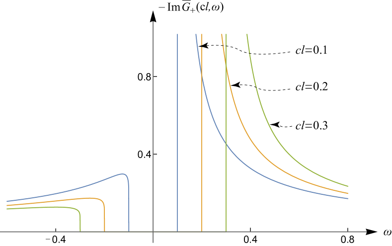
Figure 6: Fermionic spectral function $-{\rm Im}\overline{G}_{+}(l,\omega)$ as a function of the frequency $\omega$ for several $cl$. Eq. (194) is plotted for $cl=0.1$ (blue), $cl=0.2$ (purple), $cl=0.3$ (ocher). $\kappa=1$, $\alpha=0.1$, and the horizontal axis is $\omega$.

VI.2 density of states around the QCP

The density of states (DOS) is given by the integral of the fermion spectral function over the momentum ${\bm{k}}$;

$$-\rho_{+}(\omega) =\frac{1}{\pi}\int\frac{d^{3}{\bm{k}}}{(2\pi)^{3}}{\rm Im}\overline{G}^{R}_{+}(l,\omega)$$

$$=\frac{k^{2}_{F}}{c\pi^{2}}\int^{\omega}_{-\omega}{\rm Im}\overline{G}^{R}_{+}(l,\omega)\frac{d(cl)}{2\pi}.$$ (215)

The subscript ‘$+$’ refers to the DOS for the electron-type band. The following argument holds true in the same way for the hole-type band. Thus, we focus on the DOS of only the electron-type band. For small $\omega>0$ ($\omega=0$ corresponds to the Fermi level), the integral over the one-dimensional momentum $l$ is dominated by the singular spectral weight near $cl=\omega$. One can see this by dividing the integral into two regions;

$$\int^{\omega}_{-\omega}{\rm Im}\overline{G}^{R}_{+}(l,\omega)\frac{d(cl)}{2\pi}$$

$$=\int^{\omega}_{s\omega}{\rm Im}\overline{G}^{R}_{+}(l,\omega)\frac{d(cl)}{2\pi}+\int^{s\omega}_{-\omega}{\rm Im}\overline{G}^{R}_{+}(l,\omega)\frac{d(cl)}{2\pi}.$$ (216)

Here ‘$s$’ is a positive constant smaller than 1. Since the integrand increases monotonically in $cl$ for small positive $\omega$ (Fig. 2), the second term can be bounded from above;

$$-\int^{s\omega}_{-\omega}{\rm Im}\overline{G}^{R}_{+}(l,\omega)\frac{d(cl)}{2\pi}$$

$$\ \ <-\frac{(1+s)\omega}{2\pi}{\rm Im}\overline{G}^{R}_{+}(cl=s\omega,\omega)={\cal O}\bigg{(}\frac{1}{|\log\omega|^{\frac{3}{2}}}\bigg{)}.$$ (217)

Here we set $cl=s\omega$ in Eqs. (194,201) and assume that $\omega$ is sufficiently small;

$$\lim_{\omega\rightarrow 0}|A|=|\log\omega|+\cdots,\ \lim_{\omega\rightarrow 0}\overline{A}=1,\ \ \lim_{\omega\rightarrow 0}\overline{B}=-\frac{\pi}{4|A|^{2}},\ \$$

$$\lim_{\omega\rightarrow 0}\overline{C}=\frac{1}{\sqrt{2\alpha|A|}},\ \ \lim_{\omega\rightarrow 0}\overline{D}=-\frac{1}{\sqrt{2\alpha|A|}}\frac{\pi}{4|A|},$$

$$\lim_{\omega\rightarrow 0}(\overline{A}\!\ \overline{D}-\overline{B}\!\ \overline{C})=-\frac{\pi}{4\sqrt{2\alpha}|\log\omega|^{\frac{3}{2}}}+\cdots.$$ (218)

Meanwhile, for those $s$ close to 1 ($1-s$ is small but finite), the integrand of the first term in Eq. (216) can be approximated by the asymptotic form given in Eq. (208);

$$\int^{\omega}_{s\omega}(-){\rm Im}\overline{G}^{R}_{+}(l,\omega)\frac{d(cl)}{2\pi}$$

$$\ \ \simeq\sqrt{\frac{1}{\alpha}}\frac{\pi}{2}\int^{(1-s)\omega}_{0}\frac{d\eta}{2\pi}\frac{1}{\eta}\frac{1}{|\log\eta|^{\frac{3}{2}}}=\sqrt{\frac{1}{\alpha}}\frac{1}{2}\frac{1}{|\log\omega|^{\frac{1}{2}}}+\cdots.$$ (219)

For small $\omega$, Eq. (219) clearly dominates over Eq. (217). Thus, the DOS takes the following scaling form;

$$\rho_{+}(\omega)\propto\frac{k^{2}_{F}}{c\sqrt{\alpha}}\frac{1}{|\log\omega|^{\frac{1}{2}}}+\cdots.$$ (220)

Eq. (220) shows how the multiple-band Fermi system acquires a band gap when the boson system undergoes the quantum phase transition (Fig. 7). The result shows that the density of states at the Fermi level $E_{F}$ ($\omega=0$) is zero at the QCP (‘pseudo-gap’ behaviour).

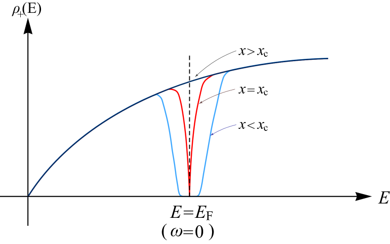
Figure 7: Schematic picture of the density of states (DOS) for electron-type energy band near the quantum critical point. For $x>x_{c}$, the DOS is finite at $E=E_{F}$ (FL phase), while for $x<x_{c}$, the DOS has a finite band gap (band insulator phase). At the QCP ($x=x_{c}$), the DOS shows a pseudo-gap behaviour; $\rho(E)\propto 1/|\log|[E-E_{F}]||^{\frac{1}{2}}$.

When the temperature $T$ is finite, $\omega$ in Eq. (220) is replaced by $T$ and the DOS at the Fermi level becomes finite;

$$\rho_{+}(\omega\simeq 0,T\neq 0)\propto\frac{k^{2}_{F}}{c\sqrt{\alpha}}\frac{1}{|\log T|^{\frac{1}{2}}}+\cdots.$$ (221)

One can see this straightforwardly, by taking the momentum integral of the spectral function at $T\neq 0$; Eq. (213).

VII conclusion

In this paper, we have studied a Fermi system with a pair of electron and hole Fermi surfaces (FS), whose coupling is mediated by a critical U(1) $\phi^{4}$ boson field. Due to the presence of the finite volume of the FS, low-energy kinematics of the fermionic excitation and that of the bosonic excitations are quite distinct from each other in the momentum space Yamamoto and Si (2010). The low-energy fermionic excitations are constrained around the FS, while the low-energy bosonic excitations are restricted around the zero-momentum point in the momentum space. Due to this geometrical distinction of the two low-energy kinematics, a naive momentum-shell Wilsonian renormalization group (RG) analysis could overlook important renormalization effects in the fermion-boson coupled model.

To avoid this difficulty, we employ in this paper a field-theoretical renormalization group analysis, where the UV cutoff dependence (UV divergent behaviour) in the vertex functions are systematically included into renormalizations of the field operator amplitudes and physical quantities. Thereby, the renormalized vertex function is given as a solution of the homogeneous Callan-Symanzik (CS) equation. By solving the CS equation in favor for the two-point fermion’s Green function, we obtain the low-energy asymptotic form of the fermion’s spectral function and density of states (DOS) at the quantum critical point (QCP). The analysis reveals that at the QCP, the Fermi velocities of the two FSs are renormalized into a same critical velocity as a boson velocity, and the fermion’s DOS shows a pseudo-gap behaviour with the logarithmic energy dependence; the DOS at the QCP vanishes toward $E=E_{F}$ with $1/|\log|E-E_{F}||^{\frac{1}{2}}$. Since $|E-E_{F}|$ and the temperature $T$ has the same scaling dimension around the $T=0$ QCP, the fermion’s DOS at the Fermi level will be also scaled as $1/|\log T|^{\frac{1}{2}}$ in a finite-$T$ side of the QCP. We expect that this log-$T$ dependence of the DOS manifest itself in various physical quantities in the quantum critical regime. Such are the electronic contribution of the specific heat and magnetic susceptibility. Namely, being proportional to the DOS at the Fermi level, the electronic contribution of the specific heat and Pauli paramagnetic susceptibility must be also scaled by $1/|\log T|^{\frac{1}{2}}$ in the high-$T$ region of the QCP.

Appendix A Callan-Symanzik equation for the boson Green’s function and boson’s spectral function at QCP

In this appendix, the CS equation for the two-point boson Green’s function will be derived at the quantum critical point (QCP) and it is solved in favor for the boson Green’s function. Out of the solution, the boson’s spectral function is obtained at the QCP. As in Sec. VA, let us begin with the relation between the bare and renormalized function;

$$Z^{-1}_{\phi}(m^{2}=0,c^{2},\cdots,\lambda,\kappa,\Lambda)\overline{G}^{-1}_{\phi}(q;c^{2},\cdots,\lambda,\kappa)$$

$$\ \ \hskip 28.45274pt=G^{-1}_{\phi}(q;m^{2}_{0},c^{2}_{0},\cdots,\lambda_{0},\Lambda).$$ (222)

The $\kappa$-derivative of Eq. (169) leads to the following inhomogeneous equation,

$$\Big{\{}\frac{\partial}{\partial\ln\kappa}+\beta_{c}\frac{\partial}{\partial c}+\sum_{\sigma=\pm}\beta_{v_{\sigma}}\frac{\partial}{\partial v_{\sigma}}+\beta_{g}\frac{\partial}{\partial g}+\beta_{\lambda}\frac{\partial}{\partial\lambda}$$

$$-\gamma_{\phi}\Big{\}}\overline{G}^{-1}_{\phi}(q;m^{2}=0,c^{2},\cdot,\lambda,\kappa)=\frac{\partial m^{2}_{0}}{\partial\ln\kappa}\frac{\partial G^{-1}_{\phi}}{\partial m^{2}_{0}}.$$ (223)

Note that in the leading order in $g^{2}$ and $\lambda$, the $\gamma$ function for the boson Green’s function is zero; $\gamma_{\phi}={\cal O}(g^{4},g^{2}\lambda,\lambda^{2})$. Meanwhile, the right hand side of Eq. (223) has a finite leading-order contribution, because $\partial G^{-1}_{\phi}/\partial m^{2}_{0}=1+{\cal O}(g^{2},\lambda)$. Thus, the CS equation takes an inhomogeneous form,

$$\Big{\{}\frac{\partial}{\partial\ln\kappa}+\sum_{\sigma=\pm}\beta_{v_{\sigma}}\frac{\partial}{\partial v_{\sigma}}+\beta_{g}\frac{\partial}{\partial g}\Big{\}}\overline{G}^{-1}_{\phi}(q,c^{2},\cdot,\kappa)$$

$$\ \ \ \ \hskip 14.22636pt=-\frac{g^{2}k^{2}_{F}}{\pi^{2}(v_{+}+v_{-})}+{\cal O}(g^{4},g^{2}\lambda,\lambda^{2}).$$ (224)

Here we also omitted $\partial_{\lambda}$ in the left hand side, which leads to terms on the order of ${\cal O}(\lambda^{2})$; $\beta_{\lambda}\propto{\cal O}(\lambda^{2})$. In the following, this equation will be solved in favor for the two-point boson Green’s function.

With $v_{\pm}=c$, the CS equation for the two-point boson vertex function is given by

$$\Big{\{}\frac{\partial}{\partial\ln\kappa}+\beta_{g}(g)\frac{\partial}{\partial g}\Big{\}}\overline{G}^{-1}_{\phi}(q;g,\kappa)=-\frac{g^{2}k^{2}_{F}}{2\pi^{2}c}.$$ (225)

Henceforth, we recover the implicit $k_{F}$-dependences in $\overline{G}_{\phi}$. According to Eq. (106), we will expand $\overline{G}^{-1}_{\phi}$ in the powers of $k^{2}_{F}$;

$$\overline{G}^{-1}_{\phi}(q;g,\kappa)= \overline{G}^{-1}_{\phi,(0)}(q;g,\kappa)+k^{2}_{F}\overline{G}^{-1}_{\phi,(1)}(q;g,\kappa)$$

$$+k^{4}_{F}\overline{G}^{-1}_{\phi,(2)}(q;g,\kappa)+\cdots.$$ (226)

The dimensional analysis dictates that $\overline{G}_{\phi,(n)}$ has a different scaling form for different $n$;

$$\overline{G}^{-1}_{\phi,(0)}(q;g,\kappa)=r^{2}g^{-1}_{(0)}(r/\kappa,\theta;g),$$

$$\overline{G}^{-1}_{\phi,(1)}(q;g,\kappa)=g^{-1}_{(1)}(r/\kappa,\theta;g),$$

$$\overline{G}^{-1}_{\phi,(2)}(q;g,\kappa)=r^{-2}g^{-1}_{(2)}(r/\kappa,\theta;g),\cdots$$ (227)

with $q\equiv(\varepsilon,{\bm{q}})$, $c|{\bm{q}}|\equiv r\sin\theta$, $\varepsilon\equiv r\cos\theta$. Since $\beta_{g}$ has no $k_{F}$ dependence, the CS equation can be decomposed into equations at every order in $k^{2}_{F}$;

$$\left\{\begin{array}[]{l}\Big{\{}\frac{\partial}{\partial\ln\kappa}+\beta_{g}(g)\frac{\partial}{\partial g}\Big{\}}\big{(}r^{2}g^{-1}_{(0)}(r/\kappa,\theta;g)\big{)}=0,\\ \Big{\{}\frac{\partial}{\partial\ln\kappa}+\beta_{g}(g)\frac{\partial}{\partial g}\Big{\}}\big{(}g^{-1}_{(1)}(r/\kappa,\theta;g)\big{)}=-\frac{g^{2}}{2\pi^{2}c},\\ \Big{\{}\frac{\partial}{\partial\ln\kappa}+\beta_{g}(g)\frac{\partial}{\partial g}\Big{\}}\big{(}r^{-2}g^{-1}_{(2)}(r/\kappa,\theta;g)\big{)}=0,\\ \hskip 56.9055pt\cdots.\\ \end{array}\right.$$ (232)

In terms of Eq. (188), the CS equation at every order in $k^{2}_{F}$ can be solved in the leading order in $g^{2}$. The solutions are

$$\left\{\begin{array}[]{l}g^{-1}_{(0)}(r/\kappa,\theta;g)=h_{(0)}(\theta;\overline{g}),\\ g^{-1}_{(1)}(r/\kappa,\theta;g)=-\frac{\overline{g}}{2\pi^{2}c}\big{(}-t+h_{1}(\theta;\overline{g})\big{)},\\ g^{-1}_{(2)}(r/\kappa,\theta;g)=h_{(2)}(\theta;\overline{g}),\\ \hskip 56.9055pt\cdots,\\ \end{array}\right.$$ (237)

with $t\equiv\ln(r/\kappa)$. $\overline{g}$ in the right hand side is given as a function of $t$ and $g$ by Eq. (188). This gives the two-point boson vertex function as follows,

$$\overline{G}^{-1}_{\phi}(r,\theta;g,\kappa)=r^{2}h_{(0)}(\theta;\overline{g})$$

$$\ \ -\frac{\overline{g}k^{2}_{F}}{2\pi^{2}c}\big{(}-t+h_{1}(\theta;\overline{g})\big{)}+r^{-2}k^{4}_{F}h_{(2)}(\theta;\overline{g})+\cdots.$$ (238)

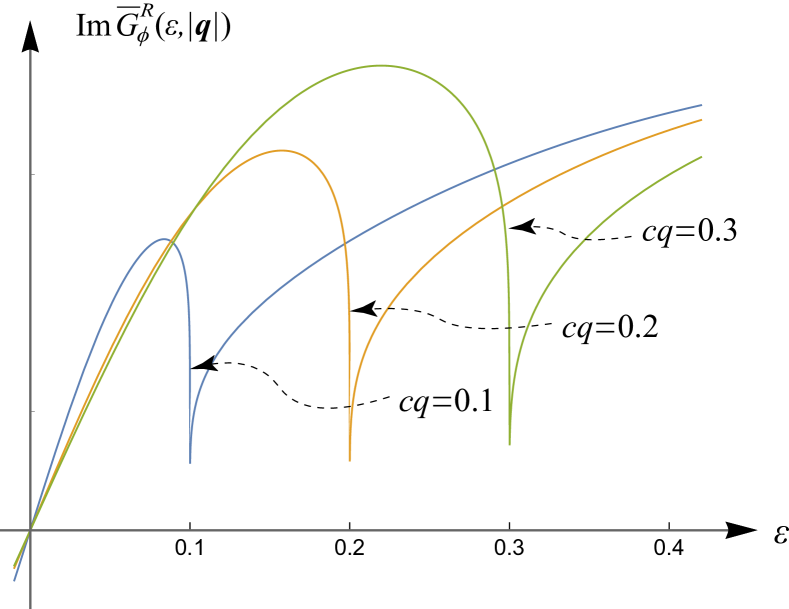
Figure 8: Bosonic spectral function ${\rm Im}\overline{G}_{\phi}(\varepsilon,|{\bm{q}}|)$ as a function of the frequency $\varepsilon$ for several $|{\bm{q}}|$. Eq. (242) is plotted for $c|{\bm{q}}|=0.1$ (blue), $c|{\bm{q}}|=0.2$ (purple), $c|{\bm{q}}|=0.3$ (ocher). $\kappa=1$, $\alpha=0.1$, $\gamma=1$, and the horizontal axis is $\varepsilon$.

According to Eqs. (238,188), $\overline{G}_{\phi}(r,\theta;g,\kappa)$ in the IR limit ($r\ll\kappa$) is determined by forms of $h_{(0)}(\theta;g)$, $h_{(1)}(\theta;g)$ and $h_{2}(\theta;g)$ for tiny $g$. To determine them for such small $g$, let us take $r=\kappa$ in Eq. (238) and expand its right hand side in small $\overline{g}(t=0;g)=g$. For small $g$, $\overline{G}_{\phi}(r=\kappa,\theta;g,\kappa)$ in the left hand side can be calculated by the second order perturbation as;

$$\overline{G}^{-1}_{\phi}(r=\kappa,\theta;g,\kappa)= \kappa^{2}-\frac{g^{2}k^{2}_{F}}{2\pi^{2}c}\Big{(}1-\frac{\theta}{\tan\theta}\Big{)}$$

$$+{\cal O}(g^{4},g^{2}\lambda,\lambda^{2}).$$ (239)

Here Eqs. (135,138,163) with $v_{\pm}=c$ are substituted into Eq.(127). A comparison between Eq. (239) and Eq. (238) at $r=\kappa$ determines $h_{(0)}(\theta;g)$, $h_{(1)}(\theta;g)$ and $h_{2}(\theta;g)$ for tiny $g$;

$$h_{(0)}(\theta;g)=1,\ \ h_{(1)}(\theta;g)=1-\frac{\theta}{\tan\theta},$$

$$h_{(2)}(\theta;g)=0,\cdots.$$ (240)

This leads to an expected result for the two-point boson vertex function in the IR limit ($r\ll\kappa$);

$$\overline{G}^{-1}_{\phi}(q;g,\kappa)=r^{2}-\frac{\overline{g}^{2}k^{2}_{F}}{2\pi^{2}c}\Big{(}-t+1-\frac{\theta}{\tan\theta}\Big{)},$$ (241)

with $q=(\varepsilon,{\bm{q}})$, $\varepsilon=r\cos\theta$, $c|{\bm{q}}|=r\sin\theta$, $t\equiv\ln(r/\kappa)$. $\overline{g}$ in the right hand side is given by $t$ and $g$ by Eq. (188). By comparing Eq. (241) with Eqs. (127,135,138,139), one can see that the $\Lambda^{2}_{B}$ term in the naive perturbation result is absorbed into the renormalization of the boson mass. ${\rm Log}\!\ \overline{\Lambda}_{F}$ and the Yukawa coupling $g$ in Eq. (127) are replaced by $\log\kappa$ and the IR-limit value of $g$, $\overline{g}$, respectively.

By an analytic continuation $i\varepsilon\rightarrow\varepsilon+i\delta$, the imaginary part of the retarded boson Green’s function (boson spectral function) is obtained as,

$$\overline{G}^{R}_{\phi}(\varepsilon,{\bm{q}}) \equiv\overline{G}_{\phi}(\varepsilon,{\bm{q}})\Big{|}_{i\varepsilon\rightarrow\varepsilon+i\delta},$$

$${\rm Im}\overline{G}^{R}_{\phi}(\varepsilon,{\bm{q}}) =\frac{\gamma\overline{F}}{(-\varepsilon^{2}+c^{2}{\bm{q}}^{2}-\gamma\overline{E})^{2}+\gamma^{2}\overline{F}^{2}},$$ (242)

where $\overline{E}$, $\overline{F}$ and $\gamma$ are given as follows,

$$\left\{\begin{array}[]{l}\overline{E}=\frac{(1-2\alpha A)(1-A)+2\alpha B^{2}+2\alpha BB^{\prime}}{(1-2\alpha A)^{2}+(2\alpha B)^{2}},\\ \overline{F}=-\frac{(1-2\alpha A)B^{\prime}+(1-2\alpha)B}{(1-2\alpha A)^{2}+(2\alpha B)^{2}},\\ \alpha\equiv\frac{g^{2}}{8\pi^{2}c^{3}},\ \gamma\equiv\frac{g^{2}k^{2}_{F}}{2\pi^{2}c},\\ A\equiv\log\big{[}\frac{\sqrt{|(c|{\bm{q}}|)^{2}-\varepsilon^{2}|}}{\kappa}\big{]},\\ B\equiv\frac{\pi}{2}\big{[}\theta(-\varepsilon-c|{\bm{q}}|)-\theta(\varepsilon-c|{\bm{q}}|)\big{]},\\ B^{\prime}\equiv-\frac{\varepsilon}{c|{\bm{q}}|}\frac{\pi}{2}\theta(c|{\bm{q}}|-|\varepsilon|).\\ \end{array}\right.$$ (249)

Note that the spectral weight is positive for $\varepsilon>0$ and negative for $\varepsilon<0$, for the low-energy boson, $|c^{2}{\bm{q}}^{2}-\varepsilon^{2}|\ll\kappa^{2}$, and for those Yukawa coupling smaller than a critical value ($\alpha<\frac{1}{2}$). Especially when $\varepsilon\rightarrow c|{\bm{q}}|+\eta$, ‘$A$’ becomes negatively large and diverges logarithmically. Due to this logarithmic divergence, the spectral weight has a ‘valley’ at $\varepsilon=c|{\bm{q}}|$ (Fig. 8), around which $\overline{E}$ and $\overline{F}$ take the following asymptotic forms,

$$\lim_{\varepsilon\rightarrow c|{\bm{q}}|}\overline{E}=\frac{1}{2\alpha},\ \ \lim_{\varepsilon\rightarrow c|{\bm{q}}|-}\overline{F}=\frac{B^{\prime}}{2\alpha A}=\frac{\pi}{2}\frac{1}{\alpha|\log|\eta||},$$

$$\lim_{\varepsilon\rightarrow c|{\bm{q}}|+}\overline{F}=-\frac{(1-2\alpha)B}{4\alpha^{2}A^{2}}=\frac{\pi}{2}\frac{1-2\alpha}{\alpha^{2}|\log|\eta||^{2}}.$$ (250)

The result shows that the delta-function peak at $\varepsilon=c|{\bm{q}}|$ for $g=0$ is wiped out completely at small but finite $g$, and is replaced by the valley. The weight has broad peaks next to the valley. Toward the bottom of the valley, the spectral weight vanishes as

$${\rm Im}\overline{G}^{R}_{\phi}(\varepsilon,{\bm{q}})=\left\{\begin{array}[]{cc}\frac{2\pi}{\gamma}\frac{\alpha}{|\log\eta|}&(\varepsilon=c|{\bm{q}}|-\eta),\\ \frac{2\pi}{\gamma}\frac{1-2\alpha}{|\log\eta|^{2}}&(\varepsilon=c|{\bm{q}}|+\eta).\\ \end{array}\right.$$ (253)

References

- Novoselov et al. (2005) K. S. Novoselov, A. K. Geim, S. V. Morozov, D. Jiang, K. M. I., I. V. Grigorieva, S. V. Dubunos, and A. A. Firsov, Nature 438, 197 (2005).
- Zhang et al. (2005) Y. Zhang, Y. W. Tan, H. L. Stomer, and P. Kim, Nature 438, 201 (2005).
- Konig et al. (2007) M. Konig, S. Wiedmann, C. Brune, A. Roth, H. Buhmann, L. W. Molenkamp, X. L. Qi, and S. C. Zhang, Science 318, 766 (2007).
- Hsieh et al. (2008) D. Hsieh, D. Qian, L. Wray, Y. Xia, Y. S. Hor, R. J. Cava, and M. Z. Hasan, Nature 452, 970 (2008).
- Xiao et al. (2010) D. Xiao, M.-C. Chang, and Q. Niu, Rev. Mod. Phys. 82, 1959 (2010).
- Qi and Zhang (2011) X.-L. Qi and S.-C. Zhang, Rev. Mod. Phys. 83, 1057 (2011).
- Hasan and Kane (2010) M. Z. Hasan and C. L. Kane, Rev. Mod. Phys. 82, 3045 (2010).
- Castro Neto et al. (2009) A. H. Castro Neto, F. Guinea, N. M. R. Peres, K. S. Novoselov, and A. K. Geim, Rev. Mod. Phys. 81, 109 (2009).
- Gross and Neveu (1974) D. J. Gross and A. Neveu, Phys. Rev. D 10, 3235 (1974).
- Herbut (2006) I. F. Herbut, Phys. Rev. Lett. 97, 146401 (2006).
- Assaad and Herbut (2013) F. F. Assaad and I. F. Herbut, Phys. Rev. X 3, 031010 (2013).
- Chubukov et al. (2008) A. V. Chubukov, D. V. Efremov, and I. Eremin, Phys. Rev. B 78, 134512 (2008).
- Fernandes et al. (2014) R. Fernandes, A. Chubukov, and J. Schmalian, Nature Physics 10, 97 (2014).
- Sun et al. (2009) K. Sun, H. Yao, E. Fradkin, and S. A. Kivelson, Phys. Rev. Lett. 103, 046811 (2009).
- Moon et al. (2013) E.-G. Moon, C. Xu, Y. B. Kim, and L. Balents, Phys. Rev. Lett. 111, 206401 (2013).
- Savary et al. (2014) L. Savary, E.-G. Moon, and L. Balents, Phys. Rev. X 4, 041027 (2014).
- Dzero et al. (2010) M. Dzero, K. Sun, V. Galitski, and P. Coleman, Phys. Rev. Lett. 104, 106408 (2010).
- Wolgast et al. (2013) S. Wolgast, i. m. c. b. u. i. e. i. f. Kurdak, K. Sun, J. W. Allen, D.-J. Kim, and Z. Fisk, Phys. Rev. B 88, 180405 (2013).
- Neupane et al. (2013) M. Neupane, N. Alidoust, S.-Y. Xu, T. Kondo, Y. Ishida, D. J. Kim, C. Liu, I. Belopolski, Y. J. Jo, T. R. Chang, H.-T. Jeng, T. Durakiewicz, L. Balicas, H. Lin, A. Bansil, S. Shin, Z. Fisk, and M. Z. Hasan, Nature Communications 4, 2991 (2013).
- Jiang et al. (2013) J. Jiang, S. Li, T. Zhang, Z. Z. Sun, F. Chen, Z. R. Ye, M. Xu, Q. Q. Ge, S. Y. Tan, X. H. Niu, M. Xia, B. P. Xie, Y. F. Li, X. H. Chen, H. H. Wen, and D. L. Feng, Nature Communications 4, 3010 (2013).
- Li et al. (2009) J. Li, R.-L. Chu, J. K. Jain, and S.-Q. Shen, Phys. Rev. Lett. 102, 136806 (2009).
- Groth et al. (2009) C. W. Groth, M. Wimmer, A. R. Akhmerov, J. Tworzydło, and C. W. J. Beenakker, Phys. Rev. Lett. 103, 196805 (2009).
- Jiang et al. (2009) H. Jiang, L. Wang, Q.-f. Sun, and X. C. Xie, Phys. Rev. B 80, 165316 (2009).
- Meier et al. (2018) E. J. Meier, F. A. An, A. Dauphin, M. Maffei, P. Massignan, T. L. Hughes, and B. Gadway, Science 362, 929 (2018), https://science.sciencemag.org/content/362/6417/929.full.pdf .
- Stutzer et al. (2018) S. Stutzer, Y. Plotnik, Y. Lumer, P. Titum, N. H. Lindner, M. Segev, M. C. Rechtsman, and A. Szameit, Nature 560, 461 (2018).
- Raghu et al. (2008) S. Raghu, X.-L. Qi, C. Honerkamp, and S.-C. Zhang, Phys. Rev. Lett. 100, 156401 (2008).
- Rachel and Le Hur (2010) S. Rachel and K. Le Hur, Phys. Rev. B 82, 075106 (2010).
- Haldane (2004) F. D. M. Haldane, Phys. Rev. Lett. 93, 206602 (2004).
- Shindou and Balents (2006) R. Shindou and L. Balents, Phys. Rev. Lett. 97, 216601 (2006).
- Shindou and Balents (2008) R. Shindou and L. Balents, Phys. Rev. B 77, 035110 (2008).
- Wang et al. (2010) Z. Wang, X.-L. Qi, and S.-C. Zhang, Phys. Rev. Lett. 105, 256803 (2010).
- Wang and Zhang (2012) Z. Wang and S.-C. Zhang, Phys. Rev. X 2, 031008 (2012).
- Chen and Son (2017) J.-Y. Chen and D. T. Son, Annals of Physics 377, 345 (2017).
- Goswami and Chakravarty (2011) P. Goswami and S. Chakravarty, Phys. Rev. Lett. 107, 196803 (2011).
- Isobe and Nagaosa (2012) H. Isobe and N. Nagaosa, Phys. Rev. B 86, 165127 (2012).
- Fradkin (1986) E. Fradkin, Phys. Rev. B 33, 3263 (1986).
- Syzranov and Radzihovsky (2018) S. V. Syzranov and L. Radzihovsky, Annual Review of Condensed Matter Physics 9, 35 (2018), https://doi.org/10.1146/annurev-conmatphys-033117-054037 .
- Armitage et al. (2018) N. P. Armitage, E. J. Mele, and A. Vishwanath, Rev. Mod. Phys. 90, 015001 (2018).
- Varma et al. (1989) C. M. Varma, P. B. Littlewood, S. Schmitt-Rink, E. Abrahams, and A. E. Ruckenstein, Phys. Rev. Lett. 63, 1996 (1989).
- Yakovenko (1993) V. M. Yakovenko, Phys. Rev. B 47, 8851 (1993).
- Lee (1989) P. A. Lee, Phys. Rev. Lett. 63, 680 (1989).
- Altshuler et al. (1994) B. L. Altshuler, L. B. Ioffe, and A. J. Millis, Phys. Rev. B 50, 14048 (1994).
- Kim et al. (1994) Y. B. Kim, A. Furusaki, X.-G. Wen, and P. A. Lee, Phys. Rev. B 50, 17917 (1994).
- Metzner et al. (2003) W. Metzner, D. Rohe, and S. Andergassen, Phys. Rev. Lett. 91, 066402 (2003).
- Rech et al. (2006) J. Rech, C. Pépin, and A. V. Chubukov, Phys. Rev. B 74, 195126 (2006).
- Fradkin et al. (2010) E. Fradkin, S. A. Kivelson, M. J. Lawler, J. P. Eisenstein, and A. P. Mackenzie, Annual Review of Condensed Matter Physics 1, 153 (2010), https://doi.org/10.1146/annurev-conmatphys-070909-103925 .
- Lee (2009) S.-S. Lee, Phys. Rev. B 80, 165102 (2009).
- Abanov et al. (2003) A. Abanov, A. V. Chubukov, and J. Schmalian, Advances in Physics 52, 119 (2003), https://doi.org/10.1080/0001873021000057123 .
- Metlitski and Sachdev (2010a) M. A. Metlitski and S. Sachdev, Phys. Rev. B 82, 075127 (2010a).
- Metlitski and Sachdev (2010b) M. A. Metlitski and S. Sachdev, Phys. Rev. B 82, 075128 (2010b).
- Fitzpatrick et al. (2013) A. L. Fitzpatrick, S. Kachru, J. Kaplan, and S. Raghu, Phys. Rev. B 88, 125116 (2013).
- Fitzpatrick et al. (2015) A. L. Fitzpatrick, G. Torroba, and H. Wang, Phys. Rev. B 91, 195135 (2015).
- Mahajan et al. (2013) R. Mahajan, D. M. Ramirez, S. Kachru, and S. Raghu, Phys. Rev. B 88, 115116 (2013).
- Fitzpatrick et al. (2014) A. L. Fitzpatrick, S. Kachru, J. Kaplan, and S. Raghu, Phys. Rev. B 89, 165114 (2014).
- Dalidovich and Lee (2013) D. Dalidovich and S.-S. Lee, Phys. Rev. B 88, 245106 (2013).
- Mandal and Lee (2015) I. Mandal and S.-S. Lee, Phys. Rev. B 92, 035141 (2015).
- Mandal (2016) I. Mandal, Phys. Rev. B 94, 115138 (2016).
- Pimenov et al. (2018) D. Pimenov, I. Mandal, F. Piazza, and M. Punk, Phys. Rev. B 98, 024510 (2018).
- Peskin and Schroeder (1995) M. E. Peskin and D. V. Schroeder, Introduction to Quantum Field Theory (Westview, 1995).
- Amit and Martin-Mayor (2005) D. J. Amit and V. Martin-Mayor, Field Theory, Renormalization Group and Critical Phenomena (World Scientific, 2005).
- Fisher et al. (1989) M. P. A. Fisher, P. B. Weichman, G. Grinstein, and D. S. Fisher, Phys. Rev. B 40, 546 (1989).
- Yang et al. (2011) K.-Y. Yang, Y.-M. Lu, and Y. Ran, Phys. Rev. B 84, 075129 (2011).
- Chen et al. (2015) C.-Z. Chen, J. Song, H. Jiang, Q.-f. Sun, Z. Wang, and X. C. Xie, Phys. Rev. Lett. 115, 246603 (2015).
- Liu et al. (2016) S. Liu, T. Ohtsuki, and R. Shindou, Phys. Rev. Lett. 116, 066401 (2016).
- Sachdev (1999) S. Sachdev, Quantum Phase Transitions (Cambridge University Press, 1999).
- José et al. (1977) J. V. José, L. P. Kadanoff, S. Kirkpatrick, and D. R. Nelson, Phys. Rev. B 16, 1217 (1977).
- Yamamoto and Si (2010) S. J. Yamamoto and Q. Si, Phys. Rev. B 81, 205106 (2010).