Few-mode Field Quantization of Arbitrary Electromagnetic Spectral Densities

Abstract

We develop a framework that provides a few-mode master equation description of the interaction between a single quantum emitter and an arbitrary electromagnetic environment. The field quantization requires only the fitting of the spectral density, obtained through classical electromagnetic simulations, to a model system involving a small number of lossy and interacting modes. We illustrate the power and validity of our approach by describing the population and electric field dynamics in the spontaneous decay of an emitter placed in a complex hybrid plasmonic-photonic structure.

Over the last years, there has been large interest in developing strategies for quantizing electromagnetic (EM) modes in open, dispersive and absorbing photonic environments. This has been motivated largely by the desire to use nanophotonic devices for quantum optics and quantum technology applications. This is a theoretical challenge, as standard ways of obtaining quantized modes are not valid in these systems Koenderink (2010); Kristensen et al. (2012). In principle, macroscopic quantum electrodynamics (QED) is the framework for such quantization in material structures described by EM constitutive relations Fano (1956); Huttner and Barnett (1992); Scheel et al. (1998); Knöll et al. (2001); Scheel and Buhmann (2008); Buhmann (2012a, b). However, in this formalism, electromagnetic fields are described by a continuum of harmonic oscillators, restricting its applicability to cases where they can be treated perturbatively or eliminated by Laplace transform or similar techniques. Work on specific structures has focused on (possibly approximately) obtaining quantized few-mode descriptions for plasmonic geometries such as a metal surface González-Tudela et al. (2014), metallic spheres Waks and Sridharan (2010); Delga et al. (2014); Rousseaux et al. (2016); Varguet et al. (2019) or sphere dimers Li et al. (2016); Cuartero-González and Fernández-Domínguez (2018). It is thus desirable to develop tractable but versatile models using only a small number of EM modes. During the past few decades, there has been extensive work in this direction, with one notable development given by pseudomode theory Imamoğlu (1994); Garraway (1997a); *Garraway1997Nonperturbative; Dalton et al. (2001).

Within nanophotonics increasing attention has recently focused on hybrid metallodielectric setups Doeleman et al. (2016); Peng et al. (2017); Gurlek et al. (2018); Franke et al. (2019), with the objective of combining the strong field confinement and enhanced light-matter interactions of plasmonic resonances with the long-lived nature (large quality factors) of microcavity or photonic crystal modes. In these systems, EM field quantization is particularly complex due to the inherent coexistence of modes with very different properties and their mutual coupling. Quasinormal modes Ching et al. (1998); Kristensen and Hughes (2014); Gurlek et al. (2018); Lalanne et al. (2018) can be useful to unveil the EM mode structure, but due to their lossy nature, direct quantization remains challenging, and has only been carried out within very limited spectral windows Hughes et al. (2018); Franke et al. (2019). A complementary technique developed very recently in the context of X-ray quantum optics is based on a partition of the physical space Lentrodt and Evers (2020).

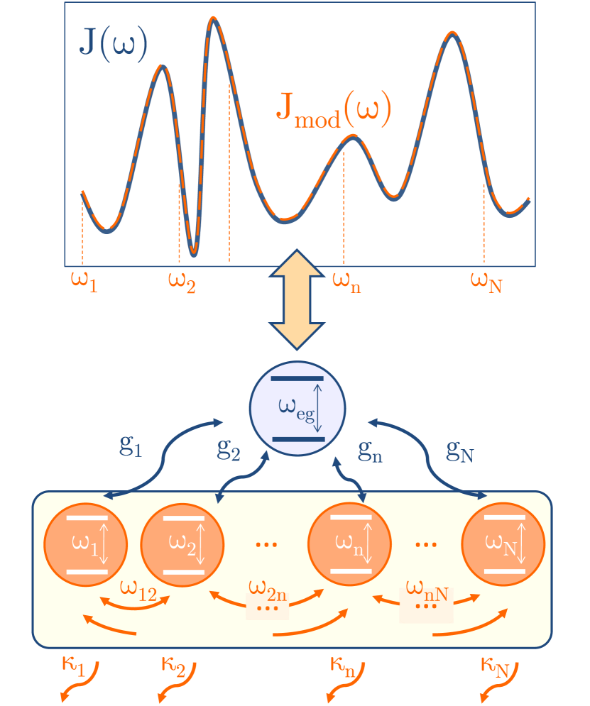
Figure 1: Sketch of the model and quantization approach. The fitting $J_{\mathrm{mod}}(\omega)$, given by Eq. (missing) 6, of an original spectral density, $J(\omega)$ (obtained usually from a numerical solution of Maxwell’s equations), provides a natural few-mode EM field quantization embodied by the master equation in Eq. (missing) 4.

It is well-known that the interaction of a single emitter with an arbitrary EM environment can be described by means of the spectral density $J(\omega)$, which encodes the density of EM modes and their coupling to the emitter. In this Letter, we present a simple and easily implementable framework for obtaining a few-mode quantum description of any given spectral density. We start from a macroscopic QED treatment, which already provides the basis of quantization in terms of a frequency continuum, and then construct a model system consisting of a discrete number of interacting modes coupled to independent flat background baths, see Fig. 1. Making use of Fano diagonalization Fano (1961); Glutsch (2002), we obtain the general form for the model spectral density, $J_{\mathrm{mod}}(\omega)$. This can be fitted to any level of accuracy to $J(\omega)$, usually obtained by means of classical EM calculations. We illustrate the power and validity of this procedure in a hybrid structure comprising a plasmonic nanocavity and a high-refractive-index microresonator. We show that our approach enables accurate calculations of any far- and near-field observables, proving that replacing the full environment by our few-mode model does not lead to a loss of information.

For a single emitter, the EM mode basis in macroscopic QED can be chosen such that the Hamiltonian becomes ($\hbar=1$ here and in the following) Buhmann and Welsch (2008); Hümmer et al. (2013); Rousseaux et al. (2016); Sánchez-Barquilla et al. (2020)

$$H_{\mathrm{f}}=H_{e}+\!\int_{0}^{\infty}\mathrm{d}\omega\left[\omega a_{\omega}^{\dagger}a_{\omega}+\hat{\mu}_{e}g(\omega)(a_{\omega}+a_{\omega}^{\dagger})\right],$$ (1)

where $H_{e}$ is the bare emitter Hamiltonian and $\hat{\mu}_{e}$ is its dipole operator, while $a_{\omega}$ are the bosonic annihilation operators of the EM mode at frequency $\omega$. These fulfill $[a_{\omega},a_{\omega^{\prime}}^{\dagger}]=\delta(\omega-\omega^{\prime})$ and correspond to the “true modes” in the nomenclature of Refs. Garraway (1997a); *Garraway1997Nonperturbative; Dalton et al. (2001). The coupling between the emitter and the EM modes is encoded by

$$g(\omega)=\sqrt{\frac{\omega^{2}}{\pi\epsilon_{0}c^{2}}\vec{n}\cdot\text{Im}\{\mathbf{G}(\vec{r}_{e},\vec{r}_{e},\omega)\}\cdot\vec{n}},$$ (2)

where $\vec{r}_{e}$ is the emitter position, $\vec{n}$ is the orientation of its dipole moment (for simplicity, we assume that all relevant transitions are oriented identically), and $\mathbf{G}(\vec{r},\vec{r}\,^{\prime},\omega)$ is the classical dyadic Green’s function. This is directly related to the spectral density of the environment, $J(\omega)=\mu^{2}g(\omega)^{2}$ for a given transition dipole moment $\mu$ Novotny and Hecht (2012).

As discussed above, Eq. (missing) 1 requires the treatment of an EM continuum. Without approximations, this is only possible with advanced and costly computational techniques, such as tensor network approaches del Pino et al. (2018); Zhao et al. . Our goal is thus to construct an equivalent system that gives rise to dynamical equations that can be solved easily. Our model environment (sketched in Fig. 1) consists of $N$ interacting EM modes with ladder operators $a_{i}$, $a_{i}^{\dagger}$, linearly coupled to the quantum emitter. Each of them is also coupled to an independent Markovian (spectrally flat) background bath. The resulting Hamiltonian is $\mathcal{H}=H_{S}+H_{B}$ with

$$H_{S} =H_{e}+\sum_{i,j=1}^{N}\omega_{ij}a^{\dagger}_{i}a_{j}+\hat{\mu}_{e}\sum_{i=1}^{N}g_{i}(a_{i}+a_{i}^{\dagger}),$$ (3a)

$$H_{B} =\sum_{i=1}^{N}\int\left[\Omega b_{i,\Omega}^{\dagger}b_{i,\Omega}+\sqrt{\frac{\kappa_{i}}{2\pi}}(b_{i,\Omega}^{\dagger}a_{i}+b_{i,\Omega}a^{\dagger}_{i})\right]\mathrm{d}\Omega.$$ (3b)

$H_{S}$ is the system (emitter + discrete modes) Hamiltonian, where the real symmetric matrix $\omega_{ij}$ describes the mode energies and their interactions, and the real positive vector $g_{i}$ describes their coupling to the emitter. The bath Hamiltonian $H_{B}$ contains both the continuous bath modes, described by the bosonic operators $b_{i,\Omega}$ and $b_{i,\Omega}^{\dagger}$ at frequency $\Omega$, and the coupling between the baths and the system, characterized by the rates $\kappa_{i}$.

The power of our approach lies in the fact that the Hamiltonian above can be analytically treated in two different ways: First, since the background baths are completely flat, the Markov approximation is exact and the dynamics described by $\mathcal{H}$ is identically reproduced, as proven recently Tamascelli et al. (2018), by a Lindblad master equation

$$\dot{\rho}=-i[H_{S},\rho]+\sum_{i}\kappa_{i}L_{a_{i}}[\rho],$$ (4)

where $\rho$ is the system density matrix and $L_{O}[\rho]=O\rho O^{\dagger}-\frac{1}{2}\{O^{\dagger}O,\rho\}$ is a standard Lindblad dissipator. Secondly, the linearly coupled system of $N$ interacting modes and continua can be diagonalized by adapting Fano diagonalization for autoionizing states of atomic systems Fano (1961), which in this context is related to the theory of quasimodes and pseudomodes Garraway (1997a); *Garraway1997Nonperturbative; Dalton et al. (2001). This strategy allows us to obtain a simple, closed expression for $J_{\mathrm{mod}}(\omega)$.

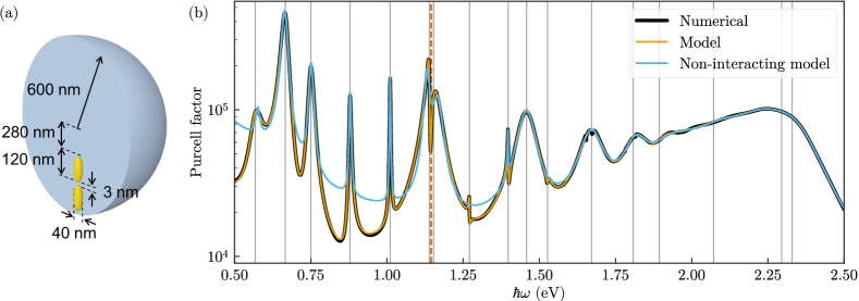
Figure 2: (a) Sketch of the model system consisting of a silver dimer nanoantenna embedded in a dielectric microsphere. (b) Purcell factor $J(\omega)/J_{0}(\omega)$ for the system (thick black line), for the fitted model described by Eq. (missing) 6 with 19 modes (orange line), and for a model without interactions with the same number of modes (light blue line). Thin gray lines indicate the energy positions of the eigenstates of $\tilde{\mathbf{H}}$ for the fitted interacting system. The red dashed line indicates the frequency of the emitter used in Fig. 3 and Fig. 4.

We first formally discretize the EM continua and rewrite Eq. (missing) 3 as

$$\mathcal{H}=H_{e}+\vec{A}^{\dagger T}\mathbf{H}\vec{A}+\hat{\mu}_{e}\vec{M}\cdot(\vec{A}+\vec{A}^{\dagger}),$$ (5)

where $\vec{A}^{T}=(a_{1},\ldots,a_{N},b_{1,\Omega_{1}},\ldots,b_{N,\Omega_{n}})$ collects the annihilation operators of both modes and baths, the matrix $\mathbf{H}$ describes their mutual couplings, and the vector $\vec{M}^{T}=(g_{1},\ldots,g_{N},0,\ldots,0)$ collects their couplings to the emitter (note that they vanish for the baths). Here, $N$ is the number of discrete modes and associated continua, while $n$ is the number of modes used to discretize each continuum. Diagonalizing $\mathbf{H}$ gives the energies $\mathcal{E}_{j}$ and eigenmodes $\vec{\psi}_{j}$ of the environment expressed in the basis of the model system, and determines the spectral density through $J_{\mathrm{mod}}(\omega)=\sum_{j}|\lambda_{j}|^{2}\delta(\omega-\mathcal{E}_{j})$, where $\lambda_{j}=\vec{M}\cdot\vec{\psi}_{j}$. Using the Sokhotski-Plemelj formula, we can write the spectral density in terms of the resolvent of Eq. (missing) 5 as ${J_{\mathrm{mod}}(\omega)=\tfrac{1}{\pi}{\rm Im}\{\vec{M}^{\dagger T}(\mathbf{H}-\omega)^{-1}\vec{M}\}}$. Applying a formalism developed for the calculation of the absorption spectrum in atomic systems Glutsch (2002) and recovering the continuum limit for the baths ($n\to\infty$), we finally obtain

$$J_{\mathrm{mod}}(\omega)=\frac{1}{\pi}\operatorname{Im}\left\{\vec{g}^{\,T}\frac{1}{\tilde{\mathbf{H}}-\omega}\vec{g}\right\},$$ (6)

where $\vec{g}^{\,T}=(g_{1},g_{2},\ldots,g_{N})$ is now an $N$-element vector and the $N\times N$ matrix $\tilde{\mathbf{H}}$ has entries $\tilde{\mathbf{H}}_{ij}=\omega_{ij}-\frac{i}{2}\kappa_{i}\delta_{ij}$. Note that we have absorbed Lamb shifts of the modes due to the coupling with the baths into the mode frequencies $\omega_{ii}$ (as we have also implicitly done in Eq. (missing) 4). We note that as required for a spectral density, this form is non-negative, i.e., $J_{\mathrm{mod}}(\omega)\geq 0$ for all $\omega$ sup .

The last step in our approach consists in using Eq. (missing) 6 to fit $J(\omega)$ for a given EM environment, which allows us to parameterize Eq. (missing) 4 for that system. Although the number of unknowns in $J_{\mathrm{mod}}(\omega)$ is relatively large ($N^{2}+2N$ real numbers for $\omega_{ij}$, $\kappa_{i}$, and $g_{i}$), the fit procedure turns out to be stable even for large numbers of modes (up to $N=19$ in the example below). A similar procedure based on the fitting of the bath correlation function has been reported as problematic recently Mascherpa et al. (2020). Note that for non-interacting modes, $\omega_{ij}=\omega_{i}\delta_{ij}$, Eq. (missing) 6 simplifies to a sum of Lorentzians of the form $J_{\mathrm{mod}}(\omega)=\sum_{i}\tfrac{g_{i}^{2}}{\pi}\frac{\kappa_{i}/2}{(\omega-\omega_{i})^{2}+\kappa_{i}^{2}/4}$. This reproduces the well-known relation between Lorentzian spectral densities and lossy modes Imamoğlu (1994); Grynberg et al. (2010) that has been widely used to quantize simpler EM environments such as plasmonic cavities in the quasi-static approximation González-Tudela et al. (2014); Delga et al. (2014); Li et al. (2016); Varguet et al. (2019). The introduction of interactions allows significantly more freedom in fitting $J_{\mathrm{mod}}(\omega)$, and in particular allows for the representation of interference effects and the associated Fano-like line shapes. In the supplemental material sup , explicit expressions of Eq. (missing) 6 for 2-4 interacting modes are presented, as well as their fitting to $J(\omega)$ in two recent studies Gurlek et al. (2018); Franke et al. (2019). In the following, we illustrate the power of our approach by considering a hybrid nanophotonic structure, with a significantly more complex spectral density.

Fig. 2(a) shows the system under study: a 600 nm radius GaP Cambiasso et al. (2017) microsphere ($\varepsilon_{\mathrm{sph}}=9$) embedding two 120 nm long silver nanorods (with permittivity taken from Ref. Rakić et al. (1998)) separated by a 3 nm gap, substantially displaced from the center of the sphere. The microsphere by itself supports many long-lived and delocalized Mie resonances, while the plasmonic dimer sustains confined surface plasmons with strongly sub-wavelength effective volumes Baumberg et al. (2019). The interaction between these different modes leads to a complex EM spectrum, shown in Fig. 2(b) through the Purcell factor $P(\omega)=J(\omega)/J_{0}(\omega)$ for an emitter located in the center of the nanorods. Here, $J_{0}(\omega)=\frac{\omega^{3}\mu^{2}}{6\pi^{2}\hbar\varepsilon_{0}c^{3}}$ is the spectral density in free space. The thick black line plots classical EM simulations performed with the Maxwell’s equation solver implemented in COMSOL Multiphysics. This Purcell factor, and the corresponding $J(\omega)$, presents a large number of maxima, with several Fano-like profiles that indicate interference effects as typical for hybrid metallodielectric systems Gurlek et al. (2018); Franke et al. (2019).

In order to obtain a stable fit of $J_{\mathrm{mod}}(\omega)$ to $J(\omega)$ despite the large number of parameters, we consider the non-interacting model (where $\omega_{ij}=\omega_{i}\delta_{ij}$) as a starting point. This fit converges rapidly by using the spectral positions, curvature, and amplitudes of the local maxima in $J(\omega)$ to obtain initial guesses for the frequencies $\omega_{i}$, loss rates $\kappa_{i}$, and coupling strengths $g_{i}$ of the non-interacting model. This gives a good fit for many of the peaks [light blue line in Fig. 2(b)], but strongly overestimates the background at lower frequencies, and fails to reproduce the Fano-like asymmetric profiles that originate from the hybridization between sphere and dimer modes. Using the non-interacting fit as a starting point for Eq. (missing) 6 leads to rapid convergence, and as shown by the orange line in Fig. 2(b), the resulting spectrum is in almost perfect agreement with the numerical Purcell factor over the full frequency range. Thus, we have constructed a compact model with a relatively small number of quantized interacting modes, each coupled to a flat background bath, that fully represents the EM environment in the nanophotonic structure in Fig. 2(a). Such an accurate fitting is not possible by means of non-interacting modes, at least not without significantly increasing the amount of modes considered. The thin grey lines in Fig. 2(b) indicate the (real part) of the eigenenergies of the matrix $\tilde{\mathbf{H}}$. These correspond to the complex resonance positions (poles) of $J(\omega)$ Dalton et al. (2001).

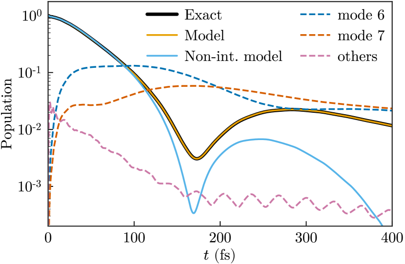
Figure 3: Emitter and mode dynamics for the spontaneous emission problem. Solid lines show the emitter excited-state population $\langle\sigma^{+}\sigma^{-}\rangle(t)$ for the exact calculation (black) and using the best-fit model with (orange) and without (light blue) interactions. Dashed lines indicate the populations $\langle\tilde{a}_{\alpha}^{\dagger}\tilde{a}_{\alpha}\rangle(t)$ of modes $\alpha=6$ (blue) and $\alpha=7$ (red) (see text for details), as well as the sum over all other mode populations (magenta).

We next demonstrate that the model system indeed gives a faithful representation of the EM environment, i.e., that the emitter dynamics with the model and with the original spectral density are equivalent. To do so, we treat the canonical spontaneous emission (Wigner-Weisskopf) problem for a two-level emitter initially in its excited state Weisskopf and Wigner (1930). We thus have $\hat{H}_{e}=\omega_{eg}\sigma^{+}\sigma^{-}$, $\hat{\mu}_{e}=\mu(\sigma^{+}+\sigma^{-})$, where $\sigma^{\pm}$ are Pauli matrices. The emitter parameters are chosen to represent InAs/InGaAs quantum dots Eliseev et al. (2000), with transition energy $\hbar\omega_{eg}=1.145$ eV, indicated by the dashed red line in Fig. 2(b), and transition dipole moment $\mu=0.55$ e nm.

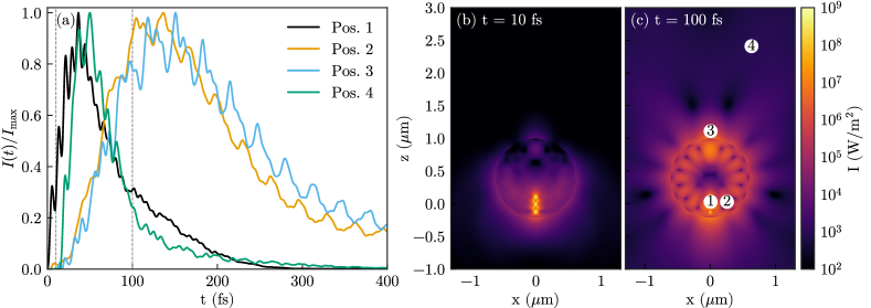
Figure 4: Electric field intensity $\langle{\vec{E}^{(-)}(\vec{r})\cdot\vec{E}^{(+)}(\vec{r})}\rangle$ for the initially excited emitter as in Fig. 3. (a) Field intensity at four points, shown by numbered white circles in panel (c), normalized to their maximum values $I_{\max}$, given by $2.0\cdot 10^{8}$ W/m², $1.8\cdot 10^{6}$ W/m², $1.1\cdot 10^{6}$ W/m², and $4.0\cdot 10^{3}$ W/m², respectively. (b) Field intensity distribution in the $x$-$z$ plane at time $t=10$ fs, and (c) at $t=100$ fs.

Since in the Wigner-Weisskopf problem, there is at most one excitation in the system (either in the emitter or in one of the EM modes), it can be solved easily for arbitrary spectral densities Grynberg et al. (2010). The exact excited-state population $\langle\sigma^{+}\sigma^{-}\rangle(t)$ obtained through this approach is shown in Fig. 3 (thick black line). The emitter dynamics in the model Lindblad master equation Eq. (missing) 4 is obtained using QuTiP Johansson et al. (2012); *Johansson2013. The excited-state population in the full model (orange line) reproduces the exact results perfectly, while the non-interacting model (light blue) fails to do so and shows significant deviations from the correct result after about $100$ fs.

In order to gain further insight into the relevance and meaning of the discrete modes obtained in our fit, we also show the populations of the modes $\tilde{a}_{\alpha}$ obtained by diagonalizing $\omega_{ij}$. Since $\omega_{ij}$ is a real symmetric matrix, this corresponds to an orthogonal transformation of the modes $a_{i}$, with $\tilde{a}_{\alpha}=\sum_{i}V_{\alpha i}a_{i}$ . The dashed lines in Fig. 3 show the mode populations of modes $\tilde{a}_{6}$ and $\tilde{a}_{7}$, which we find to be the only significantly populated modes for the chosen emitter parameters. They are exactly the modes close to resonance to the emitter frequency, $\tilde{\omega}_{6}=1.129$ eV and $\tilde{\omega}_{7}=1.149$ eV (see Fig. 2). The sum over all other mode populations, shown as a dashed magenta line in Fig. 3, remains small during the whole propagation. This demonstrates that our approach also allows the identification of the relevant modes in the dynamics.

Finally, we show that although the model system is written in terms of discrete lossy modes, it retains the full information about the EM near and far field. The electric field operator for the modes $a_{\omega}$ within the formulation we use, Eq. (missing) 1, can be written as Feist et al. (2020)

$$\vec{E}^{(+)}(\vec{r})=\int_{0}^{\infty}\vec{\mathcal{E}}(\vec{r},\omega)a_{\omega}d\omega,$$ (7)

where the field mode profile is given by

$$\vec{\mathcal{E}}(\vec{r},\omega)=\frac{\hbar\omega^{2}}{\pi\epsilon_{0}c^{2}g(\omega)}\operatorname{Im}\{\mathbf{G}(\vec{r},\vec{r}_{e},\omega)\}\cdot\vec{n}.$$ (8)

The calculation then proceeds by solving the Heisenberg equations of motion for the mode operators $a_{\omega}(t)$, which can be formally integrated to yield

$$a_{\omega}(t)=a_{\omega}(0)e^{-i\omega t}-ig(\omega)\int_{0}^{t}\hat{\mu}_{e}(t^{\prime})e^{-i\omega(t-t^{\prime})}\mathrm{d}t^{\prime}.$$ (9)

Inserting into Eq. (missing) 7 and defining the temporal kernel

$$\vec{K}(\vec{r},\tau) =\frac{\hbar}{\pi\epsilon_{0}c^{2}}\int_{0}^{\infty}\omega^{2}\operatorname{Im}\{\mathbf{G}(\vec{r},\vec{r}_{e},\omega)\}\cdot\vec{n}\,e^{i\omega\tau}\mathrm{d}\omega$$ (10)

gives compact expressions for, e.g., the electric field intensity

$$\langle{\vec{E}^{(-)}\cdot\vec{E}^{(+)}}\rangle=\int_{0}^{t}\mathrm{d}t^{\prime}\int_{0}^{t}\mathrm{d}t^{\prime\prime}\langle\hat{\mu}_{e}(t^{\prime})\hat{\mu}_{e}(t^{\prime\prime})\rangle\\ \vec{K}(\vec{r},t-t^{\prime})\vec{K}^{*}(\vec{r},t-t^{\prime\prime}),$$ (11)

where, for simplicity, we have assumed that the field is initially in the vacuum state.

Eq. (missing) 11 enables the calculation of the field intensity anywhere in space through the emitter correlation functions, which can be easily obtained from Eq. (missing) 4. This is displayed for the spontaneous emission case of Fig. 3 in Fig. 4, with panel (a) showing the temporal dependence of the electric field intensity at various points in space, with locations indicated by numbered white circles in panel (c). The intensities at each point are normalized to their maximum value, which is given in the figure caption. Panels (b) and (c) show snapshots of the field intensity profile in space at $t=10$ fs (b) and $t=100$ fs (c). A movie showing the full field distribution evolving in time is available in the supplemental material sup . We note explicitly that in this spontaneous emission problem, there is no coherent field, $\langle\vec{E}^{(+)}+\vec{E}^{(-)}\rangle$, and it is thus necessary to calculate the field intensity to observe the emission dynamics. Interestingly, the dynamics at points (1), next to the emitter, and (4) in the far-field (at a distance of $1.5~{}\mu$m from the emitter), are quite similar, reaching their maximum value within a few tens of femtoseconds and then decaying rapidly. In contrast, points (2) and (3) inside and just outside the dielectric sphere (but at some distance to the nanorod dimer) show a much slower build-up and decay of the field intensity in time. The comparison against Fig. 3 reveals that the largest contribution to the field intensity at positions 2 and 3 is given by the hybrid modes 6 and 7, while the initial fast decay is due to the contribution of other modes and leads to an intense initial pulse radiated from the system, as seen at position 4.

To conclude, we have presented a simple and insightful procedure to quantize the electromagnetic field in arbitrary nanophotonic systems. Our approach works at the level of the spectral density, calculated through the solution of Maxwell’s equations. This is fitted to a model spectral density, obtained through Fano diagonalization and involving only a small number of lossy and interacting electromagnetic modes. This makes it possible to construct and parameterize a few-mode master equation accurately describing the interaction of a quantum emitter with the original EM environment. We have illustrated the power and validity of our ideas by calculating the spontaneous emission population dynamics and near- and far-field intensity for an emitter placed within a hybrid structure comprising a dielectric microresonator and a plasmonic cavity. Our findings offer a versatile and easily implementable framework for the theoretical description of quantum nano-optical phenomena with Dyadic Green’s function calculations as the single input.