Custom Tailored Suite of Random Forests for Prefetcher Adaptation

Furkan Eris, Sadullah Canakci, Cansu Demirkiran, and Ajay Joshi
Department of Electrical and Computer Engineering, Boston University
{fe, scanakci, cansu, joshi}@bu.edu

Abstract

To close the gap between memory and processors, and in turn improve performance, there has been an abundance of work in the area of data/instruction prefetcher designs. Prefetchers are deployed in each level of the memory hierarchy, but typically, each prefetcher gets designed without comprehensively accounting for other prefetchers in the system. As a result, these individual prefetcher designs do not always complement each other, and that leads to low average performance gains and/or many negative outliers. In this work, we propose SuitAP (Suite of random forests for Adaptation of Prefetcher system configuration), which is a hardware prefetcher adapter that uses a suite of random forests to determine at runtime which prefetcher should be ON at each memory level, such that they complement each other. Compared to a design with no prefetchers, using SuitAP we improve IPC by 46% on average across traces generated from SPEC2017 suite with $\sim 12$ KB overhead. Moreover, we also reduce negative outliers using SuitAP.

Index Terms:

Prefetchers, Machine Learning, Hardware Adapters

1 INTRODUCTION

The memory wall is a well-known problem in computer architecture [17]. One method used to combat the memory wall is data/instruction prefetching. To this end, computer architects have developed many different hardware prefetchers [9]. Today’s processors consists of multiple prefetchers at each level in the memory hierarchy [7, 10]. The use of these prefetchers can lead to high average IPC gain, but can have some applications losing performance. Our experiments show that we have large negative outliers even in the current state-of-the-art prefetchers such as Bingo [5] and IPCP [14], when they are used with other prefetchers. This case is exacerbated when individual prefetchers are designed without accounting for the other prefetchers in the system. Multiple challenges arise from the interactions between the multiple prefetchers – 1) Each prefetcher tracks a specific type of traffic. For example, a stride prefetcher tracks strided accesses for a single stride, and it uses thresholds tuned for the average strided sequences. For applications that do not have strided accesses, this stride prefetcher may be suboptimal, leading to cache thrashing. In a prefetching system consisting of multiple prefetchers, this issue is more pronounced because the architectural resources are shared among all prefetchers; and 2) Different prefetchers latch onto memory access patterns at different speeds, and so a prefetcher’s behavior over time can be affected by the traffic of the other prefetchers. These differences in temporal behavior can cause faulty synchronization among prefetchers. Variations in the accuracy of each prefetcher and faulty synchronization can lead to a drop in performance. Essentially, prefetchers compete for resources, and at times, sabotage each other. To validate our argument, we generate traces from SPEC2017 benchmarks and run these traces using different prefetchers at various memory levels. We observe that the performance swing between the best and worst prefetcher system configuration (PSC)¹¹1A PSC specifies which prefetcher is switched ON at each level of the memory in the system. A PSC is denoted as prefetcher-in-L1I$)-(prefetcher-in-L1D$)-(prefetcher-in-L2$)-(prefetcher–in-LL$). The prefetchers available at each level are provided in Figure 1. can be very large (up to 642%). One way to address this problem is one could switch ON a subset of prefetchers that complement each other and are best for a given program phase.

To achieve the highest possible gain in application performance, we propose using machine learning (ML) to determine the best PSC at runtime. Contrary to the prior work [13], in our approach, we train our ML model to increase the overall processor IPC instead of training the model to improve the accuracy. We adapt a multi-label classification approach for prefetcher adaptation, where we leverage the implicit ranking among PSCs for each application to train our ML model to catch performance outliers. We train a unique random forest per PSC to create a suite of random forests. We use hardware-invariant events as our features. In particular, we choose events that are not affected by the choice of PSCs. We design our ML model with the hardware overhead in mind and aim to maximize IPC with minimum overhead. The contributions of our work are: $\bullet$ Design - We design SuitAP, a hardware adapter, which uses a suite of random forests to determine the PSC at runtime. SuitAP is non-invasive and complements any prefetcher design or heuristic. We leverage hardware-invariant events to train SuitAP to make it agnostic of the changing processor conditions. $\bullet$ Evaluation - We train SuitAP to maximize processor performance instead of accuracy. We use only 10% of the data for training to prevent overfitting and design SuitAP with a low hardware overhead ( $\sim 12$ KB). We ensure SuitAP reduces negative performance outliers. For the traces generated from SPEC2017 benchmarks, SuitAP achieves an average performance gain of over 46% compared to a system with no prefetching.

2 Related Work

Broadly, heuristic methods based on human intuition have been used in the past for designing hardware adapters for prefetcher systems[8]. Heuristic-based approaches are typically comprised of simple rules that designers have found based on intuitions gained from experimentation. While these heuristic methods improve processor performance, they are not optimal and leave performance on the table.

Recently, ML methods have been gaining traction in place of heuristic methods for prefetcher adaptation [6, 13, 12, 11]. These methods are capable of extracting the non-intuitive interactions between the different prefetchers. Prior ML methods on prefetcher adaptation configure or train the adapter using the static preset PSC and with small datasets [13, 12, 6]. Using an ML model trained using only the static preset PSC would make sense if the prefetcher system always stays in the static preset PSC at runtime. However, the PSC changes over time and it could affect the characteristics of the E-PTI²²2E-PTI corresponds to the average number of occurrences of a hardware event per thousand instructions. We use E-PTI as the features of our ML model. values collected at runtime. These characteristics could be different from the characteristics of the E-PTI values corresponding to the static preset PSC. If we use an ML model trained only based on the E-PTI values of the static preset PSC, it will lead to a sub-optimal choice of PSC at runtime. When training the ML model, we need to account for the fact that a prefetcher system can be in any one of its $N_{psc}$ possible configurations. To address this concern we train our ML model using hardware-invariant events as features.

We observe a wide variation in the complexity of the ML algorithms used in prior work. Some of the algorithms are simple and show good results because they either use small datasets or use datasets that do not accurately portray the runtime environment. As a result, these algorithms can not achieve good accuracy at runtime [13, 12]. Other algorithms, such as neural networks, are too complex and do not scale well with the size of the dataset [6]. Moreover, some prior works focus on hardware adaptation only from the perspective of accuracy without worrying about the hardware implementation [13, 12, 11].

In our work, we jointly account for accuracy and hardware when designing SuitAP. SuitAP is complex enough to provide good accuracy on a wide variety of micro-behavior. At the same time, SuitAP is not too complex to implement in hardware and scales well with the number of prefetchers and the size/complexity of the dataset.

3 SuitAP Design

3.1 SuitAP System Level Overview

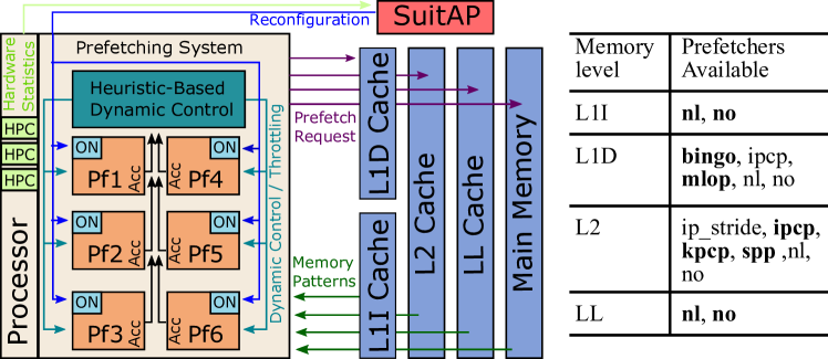
Refer to caption — Figure 1: System-level view of an example prefetching system that uses SuitAP, and prefetchers that are available to SuitAP at each memory level. Prefetchers available to SuitAP after reducing the number of PSCs are shown in bold. Here Pf = prefetchers, nl = next line prefetcher, mlop = multi-lookahead offset prefetcher, ipcp = instruction pointer classifer-based spatial prefetcher, kpcp = kill-the-PC prefetcher, bingo = bingo prefetcher, spp = signature path prefetcher, and no = no prefetching.

In Figure 1, we show the system-level design of an example prefetching system that uses SuitAP. The prefetchers track memory access patterns and send requests to prefetch data from main memory to LL$, from LL$ to L2$, and from L2$ to L1$. These prefetchers can sometimes act overly aggressively, and can adversely affect each other, in turn leading to loss of application performance. There are many heuristics-based mechanisms that use accuracy of the prefetchers or memory bandwidth utilization to throttle prefetchers in such adverse scenarios [8]. SuitAP works as a meta-controller and complements these heuristics-based throttling mechanisms. At runtime, it periodically updates the PSC i.e. it sets which prefetcher should be ON and which should be OFF at each level in the memory hierarchy, and allows each prefetcher to continue to use its associated heuristic-based throttling mechanism. To update the PSC, SuitAP uses an ML model with the E-PTI values of specific events as inputs to determine the next PSC. Effectively, throttling mechanisms are used in prefetchers to regulate the short-term behavior of the prefetchers, while SuitAP controls the longer-term system-level behavior using a more complicated ML-based approach.

3.2 SuitAP Algorithm

3.2.1 Suite of Random Forests vs. Monolithic Tree

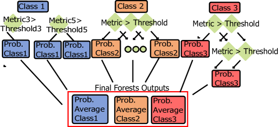
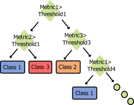
We use multi-label classification for our ML model and implement it using decision trees due to their simpler implementation. We consider the following two types of decision trees (see Figure 2): (i) Monolithic tree – Here we train a single tree for all classes. We split the tree such that we maximize the accuracy across all classes in unison instead of maximizing the accuracy of each class separately; and (ii) Suite of random forests – Here we train a custom random forest per class i.e. per PSC. As a result, we allow each forest to optimally split at locations that are unique to that class. When using a monolithic tree, at runtime, we traverse down the tree to a leaf corresponding to the next best PSC. In a suite of random forests, we have multiple trees per forest and leaves of a tree specify the probability that the PSC associated with that forest is the next best configuration. For each forest, we calculate the average of the probability values obtained from all the trees in the forest, and then choose the PSC with the highest probability. We choose suite of random forests over monolithic tree because it provides better accuracy.

In our classification problem, for a given application phase, there is an implicit ranking among the PSC choices based on the IPC of each PSC i.e. each class. This ranking shows that sometimes an application phase is indifferent to the PSC, and at other times, it is very sensitive with as much as $642\%$ change in IPC. Thus, we would like to note that the accuracy of classification does not always translate to an improvement in overall IPC. Even when classified perfectly, the application phases that are indifferent to PSC do not see a change in the overall IPC. For the application phases that are very sensitive to PSC, we can have large IPC gains or losses.

3.2.2 Training SuitAP

We train SuitAP using a diverse set of traces generated from SPEC2017 benchmarks. Consider the case where we have a single prefetcher, $Pf$ , at only one memory level. Here $N_{psc}=2$ with $Pf$ =OFF or $Pf$ =ON as the two PSCs. For two consecutive instruction windows, we will have $N_{psc}^{2}=4$ possible scenarios: (i) $Pf$ =OFF for both windows, (ii) $Pf$ =ON for the first window then OFF for the second, (iii) $Pf$ =OFF for the first window then ON for the second, and (iv) $Pf$ =ON for both windows. With $N$ number of instruction windows and $N_{app}$ number of applications, the number of different possible application behavior scenarios will then be $N_{app}*N_{psc}^{N}$ . When $N$ increases, the number of different scenarios will increase exponentially. Accounting for each unique scenario during training is not feasible.

TABLE I: Hardware-level events used by SuitAP.

Hardware Event	Properties
$RQ\_ROW\_BUFFER\_HIT$	Number of buffer hits in the read queue buffer.
$LL\$\_LOAD\_HIT$	Number of LL$ hits on load.
$BRANCH\_DIRECT\_JUMP$	Number of direct jumps on branch.
$L1I\$\_LOAD\_MISS$	Number of L1I$ load misses.
$L2\$\_PAGES\_PREFETCHED$	Number of unique L2$ pages prefetched.
$BRANCH\_CONDITIONAL$	Number of conditional branches.

TABLE II: PSCs used by SuitAP- The ticks indicate that the trace achieves top ten performance for the corresponding PSC.

PSC

638.imagick_s-10316B

649.fotonik3d_s-1176B

607.cactuBSSN_s-2421B

625.x264_s-18B

648.exchange2_s-1699B

654.roms_s-842B

600.perlbench_s-210B

628.pop2_s-17B

644.nab_s-5853B

603.bwaves_s-3699

627.cam4_s-573B

621.wrf_s-575B

631.deepsjeng_s-928B

657.xz_s-3167B

602.gcc_s-734B

641.leela_s-800B

623.xalancbmk_s-700B

619.lbm_s-4268B

605.mcf_s-665B

620.omnetpp_s-874B

nl-mlop-kpcp-nl

✓

nl-bingo-spp-nl

✓

nl-bingo-kpcp-nl

✓

no-mlop-kpcp-nl

✓

nl-mlop-spp-nl

✓

no-bingo-kpcp-nl

✓

no-bingo-spp-nl

✓

no-bingo-kpcp-no

✓

nl-bingo-ipcp-no

✓

no-bingo-ipcp-no

✓

To handle this problem we propose to use only the hardware-invariant events as our features. An example of a hardware-invariant event is the number of conditional branches, which is not affected by the choice of PSC. The use of hardware-invariant events makes it faster to generate the data set required for training SuitAP and allows us to cover all scenarios during training. For generating the training data, we use all available prefetchers in the ChampSim repository as well as the 1st (IPCP [14]), 2nd place (Bingo [5]), and 3rd (MLOP [15]) finalists of the 3rd data prefetching competition (DPC3) [2]. In the table shown in Figure 1, we show the different prefetchers we used at each memory level. We check the variance of each E-PTI value (for 180 total hardware events) for each PSC. We identify 59 events that are hardware-invariant and have a maximum variance below 10% from their mean value across all PSCs. We further reduce the number of events by eliminating the redundant events that track similar behavior. Table I shows the 6 events we use to track trace behavior.

In addition, to reduce the hardware overhead of SuitAPwe want to avoid choosing multiple PSCs covering the same traces and we want to reduce the diversity in the prefetchers. To this end, we initially run the 20 traces available in the ChampSim repository with all possible PSCs (2 L1I$ $\times$ 5 L1D$ $\times$ 6 L2$ $\times$ 2 LL$ = 120 PSCs). For each trace, we sort the PSCs based on the corresponding IPC values in descending order. We then generate a new table for each trace, where the table contains the top 10 PSC entries for the trace. We then combine these tables to form a super-table that contains the top 10 PSCs for all traces. Note that a PSC may be in the top 10 for more than one trace. For our case, we end up with 84 unique PSCs. We sort the PSCs in descending order based on the number of traces for which the PSC is in the top 10. Starting from the top, we select just enough PSCs to improve performance of all the 20 traces. We eventually end up with the 10 PSCs shown in Table II. Here the tick indicates that the PSC ranks in the top 10 for the corresponding trace. Note that performance of 638.imagick_s-10316B, 654.roms_s-842B, and 657.xz_s-3167B is agnostic of the choice of PSC. It is interesting to note that the two best PSCs from DPC3 – no-bingo-nl-nl and no-ipcp-ipcp-nl – are not in the top 10 choices for PSCs shown in Table II.

After we have identified our hardware-invariant events that will be the features and the PSCs that will be the classes of our ML model, we run the $185$ traces generated from SPEC2017 (as used by the most recent prefetcher competition) for 120M instructions and collect E-PTI values for the hardware-invariant events using 1M instruction windows. We have a warm up phase of 20M instructions before we start collecting the E-PTI values. In total we have 185(traces)*100(instruction windows per trace) = 18500 instructions windows that make up our dataset. In the dataset we have an IPC value per PSC for each instruction window as our labels. We predict the best PSC for the next instruction window.

In addition to leveraging hardware invariance, to make sure that our algorithm is not overfitting the data, we severely limit the training set size by dividing the dataset into two disjoint sets - 10% of instruction windows form the training set and the remaining 90% of the instruction windows form the testing set and perform 10-fold cross-validation on the training set. We form our suite of random forests wherein we train a separate forest for each class (i.e. each PSC) using CART (classification and regression trees) [16].

We limit the total number of nodes in SuitAP to keep the size of SuitAP smaller than L1$. With this limitation in mind, we conduct a hyper-parameter search and find that the number of estimators (trees per random forest) should be 5 and the number of nodes should be 50 per class. SuitAP is trained to find the best IPC value for the next instruction window. We would like to note that SuitAP is made up of several random forests and each forest is made up of several decision trees. This increases the tolerance of our method where even if some of the trees give wrong decisions, other trees can overcome this error.

3.3 SuitAP Hardware Design

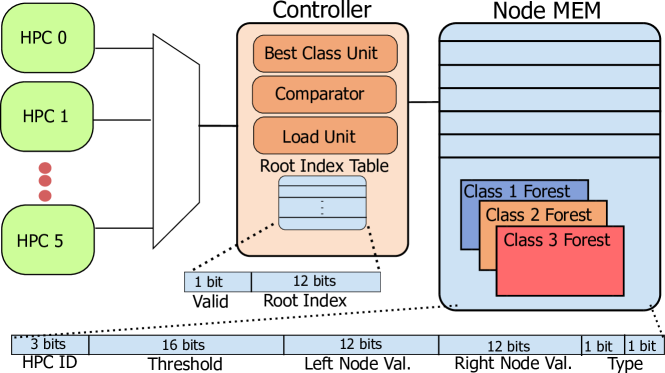
Figure 3 shows the hardware design of SuitAP. We use a single port SRAM array called Node MEM to store information about SuitAP. We load the offline-trained model into the Node MEM at startup using firmware. Each entry of Node MEM corresponds to one node in one of the random forests and it consists of the following fields: (i) A 3-bit HPC ID field that specifies which hardware-level event is used by that node to make a decision. The 3-bit encoding enables the node to use one of 6 different hardware-level events (see Table I). (ii) A 16-bit Threshold field (threshold value is determined during training), which is employed by the node to make a decision if the decision path should branch left or right. (iii) A 12-bit (for 2250 node addresses) Left Node Value(LNV) field, and (iv) a 12-bit Right Node Value(RNV) field. These LNV and RNV fields represent child node indices for internal nodes of a tree. For the leaf nodes of a tree, we use these LNV and RNV fields to indicate the probability of a class. We differentiate between child node index and probability using (v) a 1-bit Type field.

At the end of every instruction window, SuitAP calculates the probability of using each class in the next instruction window by the traversing the trees of the associated forest and using E-PTI values for the current window as inputs. For each forest, the controller in SuitAP reads the Node MEM index of the root node for the first tree from Root Index Table (RIT) and loads the Node MEM entry for the root node using a Load Unit into a register. Next, the HPC ID in the loaded Node MEM entry is used to load the corresponding E-PTI value into a second register. Then the Threshold value, stored in the first register, and E-PTI value stored in the second register are compared using the Comparator. Based on the Comparator output, we choose the left child or the right child. The Controller then uses the corresponding index value from LNV or RNV to find the next node in Node MEM. The Controller continues traversing the tree until it loads a probability value corresponding to a leaf from the Node MEM. The above steps are repeated for the remaining trees in the forest, and then we calculate the average of the probability values obtained from all the trees in that forest. The Best Class Unit in the Controller stores the ID of the class with the highest probability value. Every time the Controller finishes traversing a forest, the probability value of that forest, i.e. class, is compared with the probability value stored in the Best Class Unit using the Comparator. If the new probability value is higher than the current value, the Best Class Unit updates the probability value and the ID of the class. Once all forests have been traversed i.e. all classes have been evaluated, SuitAP chooses the entry stored in the Best Class Unit as the PSC for the next instruction window.

We determined that a maximum depth of $10$ per tree is more than sufficient to accurately determine the best PSC. In our evaluation we use a prefetcher system with $N_{psc}$ =10 (given in Table II and discussed in detail in Section 5). If we evaluate all 10 forests in series, where we will require a maximum 500 comparison operations (10 forests * 5 trees per forest * 10 comparisons = 500 comparisons), it will take less than $0.1\%$ (assuming each comparison operation takes less than a clock cycle) of the time required to execute the 1M instructions in the instruction window. Thus we end up using the chosen PSC for 99.9% of the instruction window.

We need a total of 2250 nodes to design the trees in SuitAP, and these nodes require a 12.75 KB-sized Node MEM (compared to L1$ of 64 KB). Other than Node MEM, we require a $5*N_{psc}$ -entry RIT where each entry is 13-bit wide (12 bits for the root node index and 1 valid bit), a 12-bit comparator, a load unit, and a register to store the best class information in the Controller. For the Node MEM operating at $5GHz$ , using Cacti 7.0 [3] we find that the area overhead in a $32nm$ process is roughly $0.03mm^{2}$ and the power is roughly $0.2mW$ for 500 Node MEM accesses every 1M instructions. The area and power required for the remaining components is negligible.

4 Evaluation Methodology

For our evaluation, we use ChampSim [4] to model an OoO processor and multiple prefetchers at each level in the memory hierarchy (see table in Figure 1). We use perceptron for branch predictor and least-recently used (LRU) policy for cache replacement policy. We use the default parameters in ChampSim for the rest of the processor architecture. We use traces generated from SPEC2017 [1] for performance evaluation of SuitAP.

5 Evaluation Results

Broadly, compared to a processor with no prefetchers, SuitAP provides an average performance gain of 46%. For better insight into SuitAP, we also compare the performance of (i) no-ipcp-ipcp-nl (DPC3 1st place) [14], (ii) no-bingo-nl-nl (DPC3 2nd place) [5], and (iii) SuitAP (we show the prefetchers used at each memory level by SuitAP in bold in the table found in Figure 1); against nl-mlop-kpcp-nl PSC as our experiments show that if we could choose only one PSC, then nl-mlop-kpcp-nl would be best choice for 50% of the traces. L1I$ prefetchers were not an option during the DPC3. We compared no-bingo-nl-nl with nl-bingo-nl-nl and no-ipcp-ipcp-nl with nl-ipcp-ipcp-nl and did not observe a large performance difference, therefore, we leave nl-bingo-nl-nl and nl-ipcp-ipcp-nl out of the discussion.

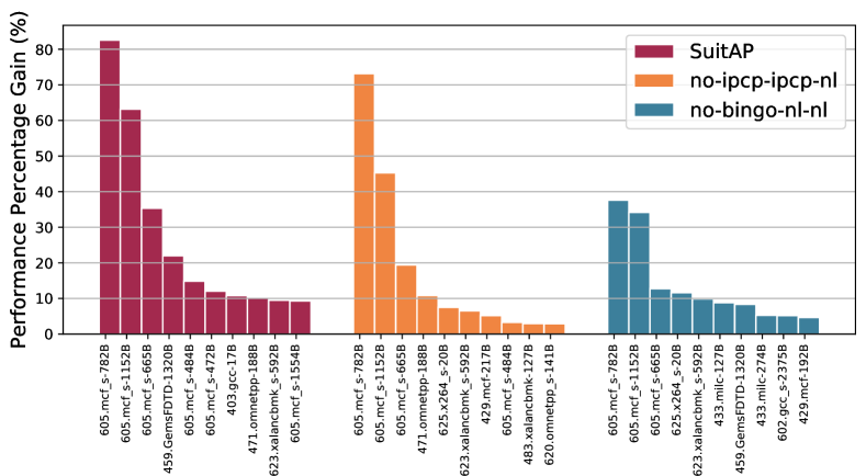
In Figure 4a we show the top ten performance gains for the two PSCs and SuitAP to understand the distribution of the performance gains. We cannot show the performance gain for all 185 traces due to space constraints. Using no-ipcp-ipcp-nl and no-bingo-nl-nl, we observe a maximum performance gain of 73.1% and 37.6%, and an average performance gain (across all 185 traces) of 0.4% and 0.43%, respectively. As we can clearly see, SuitAP beats both competitors in terms of performance gains. SuitAP has a maximum performance gain of 82.5% and an average of 2.2% across all 185 traces.

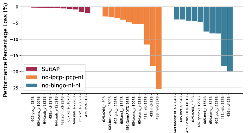
The main advantage of SuitAP is that it minimizes the negative outliers. In Figure 4b we show the ten worst trace performances for the two PSCs and SuitAP. SuitAP has a performance loss in the range of 2% to 0.3%. no-ipcp-ipcp-nl and no-bingo-nl-nl, have a performance loss in the range of 25.5% to 3% and 20% to 4%, respectively. This clearly shows that SuitAP provides us with a win-win situation, whereby we not only see a better average performance gain across all traces but also see a reduction in the performance loss for the outliers.

6 Conclusion and Future Work

In this work, we introduce SuitAP, a novel ML-based prefetcher adapter designed using custom tailored random forests. We train a dedicated random forest for each PSC, which allows the random forest to retain more information in a smaller amount of hardware. SuitAP with multiple prefetchers on each level in the memory hierarchy improves the performance of applications by 46% on average (642% peak value) when compared to a processor with no prefetching. SuitAP also reduces the negative outliers from a maximum 25.5% for ipcp and 20% for bingo performance loss in the prior work down to a 2% maximum performance loss. In the future, we plan to develop SuitAP for a manycore system where there will be co-ordination between all prefetchers in all of the cores.

References

[1] SPEC CPU^® 2017. https://www.spec.org/cpu2017/.
[2] DPC3. https://dpc3.compas.cs.stonybrook.edu/, 2019.
[3] CACTI 7.0. https://github.com/HewlettPackard/cacti, 2020.
[4] ChampSim. https://github.com/ChampSim/ChampSim, 2020.
[5] M. Bakhshalipour et al. Bingo spatial data prefetcher. Proc. HPCA, pp. 399–411, 2019.
[6] E. Bhatia et al. Perceptron-based prefetch filtering. Proc. ISCA, pp. 1–13, 2019.
[7] A . M . D. Bios. kernel developer guide (bkdg) for AMD family 10h models 00h-0fh processors, 2010.
[8] E. Ebrahimi et al. Coordinated control of multiple prefetchers in multi-core systems. Proc. MICRO, pp. 316–326, 2009.
[9] B. Falsafi and T . F. Wenisch. A primer on hardware prefetching. Synthesis Lectures on Computer Architecture, 9(1):1–67, 2014.
[10] P . . Guide. Intel® 64 and ia-32 architectures software developer‘s manual. Volume 3B: System programming Guide, Part, 2011.
[11] J. Hiebel et al. Machine learning for fine-grained hardware prefetcher control. Proc. ICPP, p. 3, 2019.
[12] V. Jiménez et al. Making data prefetch smarter: Adaptive prefetching on power7. Proc. PACT, pp. 137–146, 2012.
[13] S . w. Liao et al. Machine learning-based prefetch optimization for data center applications. Proc. SC, p. 56, 2009.
[14] S. Pakalapati and B. Panda. Bouquet of instruction pointers: Instruction pointer classifier-based spatial hardware prefetching. Proc. ISCA, pp. 118–131, 2020.
[15] M. Shakerinava et al. Multi-lookahead offset prefetching. The Third Data Prefetching Championship, 2019.
[16] D. Steinberg. Cart: classification and regression trees. The top ten algorithms in data mining, pp. 193–216. Chapman and Hall/CRC, 2009.
[17] W . A. Wulf and S . A. McKee. Hitting the memory wall: implications of the obvious. ACM CAN, 23(1):20–24, 1995.