Corotating dyonic binary black holes

Abstract

This paper is dedicated to derive and study binary systems of identical corotating dyonic black holes separated by a massless strut –two 5-parametric corotating binary black hole models endowed with both electric and magnetic charges– where the dyonic black holes carrying equal/opposite electromagnetic charges in the first/second model satisfy the extended Smarr formula for the mass including the magnetic charge as a fourth conserved parameter.

I Introduction

It is well-known that any black hole (BH) solution fulfilling the Einstein-Maxwell equations in stationary spacetimes can be described by only three conserved parameters: the mass, electric charge, and angular momentum MTW . This statement is called the no-hair conjectureIsrael0 ; CarterRobinson ; Mazur and a Kerr-Newman BH solution ENewman is the one depicted by these physical parameters. Obviously, one may bear in mind the addition of the magnetic charge as a fourth conserved parameter since it is also conserved in Einstein-Maxwell theory Bekenstein . In this context, a duality rotation (DR) studied long time ago by Carter Carter seems to be the easiest path to add the magnetic charge into the Kerr-Newman solution in order to describe a rotating dyon –a particle containing both electric and magnetic charges Schwinger –, which will satisfy an extended Smarr formula for the mass Smarr . It should be mentioned that in this approach there exists no Dirac string (DS) (or monopole hair) joined to the BH.

On the other hand, Tomimatsu Tomi via Komar integrals Komar provided simple formulas that permits the derivation of the mass formula for multi-connected horizons. In particular, in a binary BH system he found that in the absence of the global net magnetic charge there appears a DS linking the BHs, in the way of magnetic flux. In this physical scenario the global magnetic charge is eliminated once each BH is equipped with an individual magnetic charge opposite in sign but carrying the same magnitude. Naturally that, the DS vanishes if there are no magnetic charges in the solution Tomi recovering the Kerr-Newman BH description. It is worthwhile to stress the fact that there exist two approaches that allow us to add the magnetic charge into each BH; the DR Carter and the inclusion of the DS into the mass Tomi ; Galtsov .

Following Tomimatsu’s approach, in CLLM1 ; CLLM2 ; CLM has been studied the contribution of the DS into the mass formula for two counterrotating dyonic BHs held apart by a massless strut BachW ; Israel , founding that each individual angular momentum suffers additional rotation provided by the presence of the DS, in the form $J-Q_{H}Q_{B}$. However, in a later paper published by Clément and Gal’tsov Galtsov it was shown that Tomimatsu’s formulas Tomi are incorrect in the presence of both electric and magnetic charges, owing to the fact that the DS affects only the horizon mass and not the horizon angular momentum as was reported earlier in CLLM1 ; CLLM2 ; CLM , where it is necessary to adopt a constant (or gauge) in the magnetic potential in order to give equal weights to balance the horizon mass and angular momentum.

The present paper has the main goal to use Carter’s proposal Carter on the DR to derive the dyonic extensions of two corotating Kerr-Newman binary BH models previously studied in CCHV . These extended models are well represented by five physical arbitrary parameters: mass $M_{H}$, angular momentum $J_{H}$, electric charge $Q_{H}$, magnetic charge $B_{H}$, and a relative distance $R$, where all the thermodynamical properties contained inside the extended Smarr formula have been derived in a concise form. In addition, it is demonstrated that after the DR is applied, the physical Komar parameters $\{M_{H},Q_{H},B_{H},J_{H}\}$ are conserved without the need of adding any specific constant in the magnetic potential, contrary to the claim made in MankoCompean . In this regard, is also added a short description on the correct use of this gauge with the aim to include the contribution of the DS in the horizon mass, by using once again the results of CLLM2 and the ones derived within this work for corotating systems.

II Corotating dyonic binary black holes

Let us begin this section by introducing the following Ernst equations Ernst :

$$\begin{split}\left({\rm{Re}}{\cal{E}}+|\Phi|^{2}\right)\Delta{\cal{E}}&=(\mbox{\boldmath$\nabla$}{\cal{E}}+2\bar{\Phi}\mbox{\boldmath$\nabla$}\Phi)\cdot\mbox{\boldmath$\nabla$}{\cal{E}},\\ \left({\rm{Re}}{\cal{E}}+|\Phi|^{2}\right)\Delta\Phi&=(\mbox{\boldmath$\nabla$}{\cal{E}}+2\bar{\Phi}\mbox{\boldmath$\nabla$}\Phi)\cdot\mbox{\boldmath$\nabla$}\Phi,\end{split}$$ (1)

that are equivalent to Einstein-Maxwell field equations in stationary axisymmetric spacetimes, where $({\cal{E}},\Phi)$ are complex potentials given by ${\cal{E}}=f-|\Phi|^{2}+i\Psi$ and $\Phi=-A_{4}+iA^{\prime}_{3}$. We notice that Eq. (1) remain invariant under DR, in which $\Phi$ might be replaced by $\Phi e^{i\alpha}$, where $\alpha$ is a constant duality angle closely linked to the magnetic charge. On the other hand, the line element defining stationary axisymmetric spacetimes is given by Papapetrou

$$ds^{2}=f^{-1}\left[e^{2\gamma}(d\rho^{2}+dz^{2})+\rho^{2}d\varphi^{2}\right]-f(dt-\omega d\varphi)^{2},$$ (2)

where $f(\rho,z)$,$\omega(\rho,z)$, and $\gamma(\rho,z)$ are metric functions that can be obtained once one is able to solve following differential equations

$$4\gamma_{,\rho} =\rho f^{-2}\left[|{\cal{E}}_{,\rho}+2\bar{\Phi}\Phi_{,\rho}|^{2}-|{\cal{E}}_{,z}+2\bar{\Phi}\Phi_{,z}|^{2}\right]-4\rho f^{-1}(|\Phi_{,\rho}|^{2}-|\Phi_{,z}|^{2}),$$

$$2\gamma_{,z} =\rho f^{-2}{\rm{Re}}\left[({\cal{E}}_{,\rho}+2\bar{\Phi}\Phi_{,\rho})(\bar{{\cal{E}}}_{,z}+2\bar{\Phi}\Phi_{,z})\right]-4\rho f^{-1}{\rm{Re}(\bar{\Phi}_{,\rho}\Phi_{,z})},$$

$$\omega_{,\rho} =-\rho f^{-2}{\rm{Im}}({\cal{E}}_{,z}+2\Phi\bar{\Phi}_{,z}),\qquad\omega_{,z}=\rho f^{-2}{\rm{Im}}({\cal{E}}_{,\rho}+2\Phi\bar{\Phi}_{,\rho}).$$ (3)

Then we have that the explicit knowledge of the Ernst potentials $({\cal{E}},\Phi)$ fulfilling Eq. (1), will be helpful to solve Eq. (3). In order to derive the Ernst potentials as well as the metric functions in the entire space $(\rho,z)$ one can make use of Sibgatullin’s method Sibgatullin , where it is necessary to adopt first a specific form of the Ernst potentials on the symmetry axis (the axis data). In CCHV we have used the following axis data for asymptotically flat spacetimes

$${\cal E}(0,z) =\frac{z^{2}-2(M+i\mathfrak{q})z+2\Delta-R^{2}/4-\sigma^{2}-2q_{o}(Q/M)+i\delta}{z^{2}+2(M-i\mathfrak{q})z+2\Delta-R^{2}/4-\sigma^{2}+2q_{o}(Q/M)-i\delta},$$

$$\Phi(0,z) =\frac{2(Qz+\mathfrak{q}_{o})}{z^{2}+2(M-i\mathfrak{q})z+2\Delta-R^{2}/4-\sigma^{2}+2q_{o}(Q/M)-i\delta},$$

$$\sigma =\sqrt{\Delta-\frac{4\big{[}|\mathfrak{q}_{o}|^{2}-(Q/M)^{2}q_{o}^{2}\big{]}-\delta^{2}}{R^{2}-4\Delta}},\qquad\Delta=M^{2}-Q^{2}-\mathfrak{q}^{2},\qquad\mathfrak{q}_{o}=q_{o}+ib_{o},$$ (4)

with the main objective to describe corotating binary systems of identical Kerr-Newman BHs ENewman . From the aforementioned Eq. (4) after applying the Hoenselaers-Perjés procedure HP ; Sotiriou , it is possible to obtain the first Simon’s multipoles Simon , where the total mass, total electric charge, and total angular momentum of the binary system are represented by $2M$, $2Q$, and $4M\mathfrak{q}-\delta$, respectively, while the total electromagnetic dipole moment is given as $2\big{[}q_{o}+i(b_{o}+2\mathfrak{q}Q)\big{]}$. Moreover, $R$ defines a separation distance between the sources (see Fig. 1), which may be BHs if $\sigma^{2}\geq 0$ or hyperextreme sources when $\sigma^{2}<0$. In this framework, the Ernst potentials, Kinnersley potential $\Phi_{2}$ Kinnersley as well as the metric functions in the whole spacetime were obtained in Ref. CCHV ; these explicitly are

$${\cal{E}} =\frac{\Lambda+\Gamma}{\Lambda-\Gamma},\quad\Phi=\frac{\chi}{\Lambda-\Gamma},\qquad\Phi_{2}=\frac{F}{\Lambda-\Gamma},\qquad f=\frac{|\Lambda|^{2}-|\Gamma|^{2}+|\chi|^{2}}{|\Lambda-\Gamma|^{2}},\qquad\omega=4\mathfrak{q}+\frac{{\rm{Im}}\left[(\Lambda-\Gamma)\overline{\mathcal{G}}-\chi\overline{\mathcal{I}}\right]}{|\Lambda|^{2}-|\Gamma|^{2}+|\chi|^{2}},$$

$$e^{2\gamma} =\frac{|\Lambda|^{2}-|\Gamma|^{2}+|\chi|^{2}}{64\sigma^{4}R^{4}\kappa_{o}^{2}r_{1}r_{2}r_{3}r_{4}},\qquad\Lambda=2\sigma^{2}\left[R^{2}\kappa_{o}(r_{1}+r_{2})(r_{3}+r_{4})+4a(r_{1}-r_{3})(r_{2}-r_{4})\right]$$

$$+2R^{2}\left[\kappa_{o}(2\Delta-\sigma^{2})-a\right](r_{1}-r_{2})(r_{3}-r_{4})+2iR\bigg{\{}\Big{(}2\mathfrak{q}{\rm Re}(s_{+})+{\rm Im}(p_{+})\Big{)}\Big{[}R(\mathfrak{r}_{1}-\mathfrak{r}_{2})(r_{3}-r_{4})$$

$$-2\sigma\big{(}\mathfrak{r}_{1}r_{4}-\mathfrak{r}_{2}r_{3}+4\sigma r_{3}r_{4}\big{)}\Big{]}+\mathfrak{q}\kappa_{o}\Big{[}r_{1}\big{(}R^{2}r_{3}-\kappa_{o}r_{4}\big{)}-r_{2}\big{(}\kappa_{o}r_{3}-R^{2}r_{4}\big{)}-8\sigma^{2}r_{3}r_{4}\Big{]}\bigg{\}},$$

$$\Gamma =4\sigma R\left(M\Gamma_{o}-b\chi_{+}\right),\quad F=(4\mathfrak{q}+iz)\chi-i\mathcal{I},\quad\chi=-4\sigma R\left(Q\Gamma_{o}+2\mathbb{Q}\chi_{+}\right),\quad\Gamma_{o}=R\chi_{-}-2\sigma\chi_{s}+2\chi_{1+},$$

$$\mathcal{G} =2z\Gamma+8\sigma^{2}\bigg{\{}R\Big{[}2\big{(}{\rm Re}(a)-2|\mathfrak{q}_{o}|^{2}\big{)}+Q^{2}\kappa_{o}\Big{]}(r_{1}r_{2}-r_{3}r_{4})+2i\mathfrak{q}R^{2}\kappa_{o}(r_{2}r_{3}+r_{1}r_{4})+2i\Big{[}R{\rm Im}(a)+Q\xi_{0}-4\mathfrak{q}|\mathfrak{q}_{o}|^{2}\Big{]}$$

$$\times(r_{1}-r_{3})(r_{2}-r_{4})\bigg{\}}-4R^{2}\bigg{\{}\sigma\left[2a-(R-2\sigma)\Big{(}2(R+2i\mathfrak{q})s_{+}+p_{+}\Big{)}\right]+i\left(Q\xi_{o}+2Qb_{o}\kappa_{o}-4\mathfrak{q}|\mathfrak{q}_{o}|^{2}\right)\bigg{\}}(r_{1}-r_{2})(r_{3}-r_{4})$$

$$+2\sigma R\bigg{\{}4R\Big{(}2\kappa_{o}\Delta-{\rm Re}(a)\Big{)}r_{4}+\Big{[}Q(4q_{o}+QR)\kappa_{o}+4R|\mathfrak{q}_{o}|^{2}\Big{]}(r_{3}+r_{4})\bigg{\}}(r_{1}-r_{2})$$

$$+2\sigma R\bigg{\{}4R\Big{(}2\kappa_{o}\Delta-{\rm Re}(a)\Big{)}r_{2}-\Big{[}Q(4q_{o}-QR)\kappa_{o}-4R|\mathfrak{q}_{o}|^{2}\Big{]}(r_{1}+r_{2})\bigg{\}}(r_{3}-r_{4})+4M\sigma R\big{(}\kappa_{o}\chi_{+}+2R\chi_{1-}+4\sigma\chi_{p}\big{)}$$

$$-4b\sigma R(R\chi_{-}+2\sigma\chi_{s})-8\sigma R(Qb+2M\mathbb{Q})\Big{[}2\bar{\mathfrak{q}}_{o}\big{(}\mathfrak{r}_{1}-\mathfrak{r}_{2}+\mathfrak{r}_{3}-\mathfrak{r}_{4}\big{)}+Q\kappa_{o}(r_{1}-r_{2}-r_{3}+r_{4})\Big{]},$$

$$\mathcal{I} =A\Big{[}4\sigma^{2}(r_{1}-r_{3})(r_{2}-r_{4})-R^{2}(r_{1}-r_{2})(r_{3}-r_{4})\Big{]}+R\kappa_{-}\Big{[}B_{+}\kappa_{o}r_{1}-B_{-}R\mathfrak{r}_{2}\Big{]}r_{4}+R\kappa_{+}\Big{[}B_{-}\kappa_{o}r_{2}-B_{+}R\mathfrak{r}_{1}\Big{]}r_{3}$$

$$-16\sigma^{2}R\Big{\{}\Big{[}M(R+2\sigma)(\kappa_{+}+2QR)-B_{+}\mathfrak{q}_{o}\Big{]}r_{3}r_{4}-R\kappa_{o}(2M\mathbb{Q}+Qb)\Big{\}}+8\mathbb{Q}\sigma R(\chi_{1+}+\sigma\chi_{s})$$

$$+2\sigma R\Big{[}Q\big{(}2R^{2}-8\Delta+\kappa_{o}\big{)}+8i\mathfrak{q}\mathbb{Q}\Big{]}\chi_{+}+12\sigma R^{2}\mathbb{Q}\chi_{-}+8Q\sigma R(R\chi_{1-}+2\sigma\chi_{p}),\quad\kappa_{o}=R^{2}-4\sigma^{2},$$

$$\chi_{\pm} =s_{+}\mathfrak{r}_{1}-s_{-}\mathfrak{r}_{2}\pm(\bar{s}_{-}\mathfrak{r}_{3}-\bar{s}_{+}\mathfrak{r}_{4}),\quad\chi_{1\pm}=p_{+}\mathfrak{r}_{1}+p_{-}\mathfrak{r}_{2}\pm(\bar{p}_{-}\mathfrak{r}_{3}+\bar{p}_{+}\mathfrak{r}_{4}),\quad\chi_{s}=s_{+}\mathfrak{r}_{1}+s_{-}\mathfrak{r}_{2}+\bar{s}_{-}\mathfrak{r}_{3}+\bar{s}_{+}\mathfrak{r}_{4},$$

$$\chi_{p} =p_{+}\mathfrak{r}_{1}-p_{-}\mathfrak{r}_{2}+\bar{p}_{-}\mathfrak{r}_{3}-\bar{p}_{+}\mathfrak{r}_{4},\quad a=(R+2i\mathfrak{q})p_{+}-s_{+}\big{[}s_{+}-(R+2i\mathfrak{q})^{2}\big{]},\quad b=-2q_{o}(Q/M)+i(\delta-4M\mathfrak{q}),$$

$$A =4M\Big{[}\Big{(}2\mathbb{Q}+Q(R-2\sigma)\Big{)}s_{+}+2Qp_{+}\Big{]}+B_{+}\Big{[}Q\big{(}R^{2}-4\Delta\big{)}-2(R+2i\mathfrak{q})\mathfrak{q}_{o}\Big{]},\quad\kappa_{\pm}=2\mathfrak{q}_{o}-Q(R\pm 2\sigma),$$

$$B_{\pm} =\Big{[}Rs_{\pm}\pm p_{\pm}+2Q\big{(}2\bar{\mathfrak{q}}_{o}+Q(R\pm 2\sigma)\big{)}\Big{]}/M,\quad p_{\pm}=-\sigma(R^{2}-4\Delta)\pm i\big{[}2M\delta+4b_{o}Q-(R+2i\mathfrak{q}){\rm Im}(s_{\pm})\big{]},$$

$$s_{\pm} =2\Delta\pm\sigma R+i\mathfrak{q}(R\pm 2\sigma),\quad\xi_{o}=4Q\Big{[}M\delta+2b_{o}Q+\mathfrak{q}(\Delta-\sigma^{2})\Big{]}-(2b_{o}+\mathfrak{q}Q)(R^{2}-4\Delta),\quad\mathbb{Q}=\mathfrak{q}_{o}+2i\mathfrak{q}Q,$$

$$\mathfrak{r}_{1,4} =(R-2\sigma)r_{1,4},\quad\mathfrak{r}_{2,3}=(R+2\sigma)r_{2,3},\quad r_{1,2}=\sqrt{\rho^{2}+\left(z-R/2\mp\sigma\right)^{2}},\quad r_{3,4}=\sqrt{\rho^{2}+\left(z+R/2\mp\sigma\right)^{2}},$$ (5)

where $r_{n}=\sqrt{\rho^{2}+(z-\alpha_{n})^{2}}$ are the distances from the value $\alpha_{n}$ defining the location of the source to any point $(\rho,z)$ outside the symmetry axis as shown in Fig. 1. On the other hand, it is necessary to impose the next axis condition

$$\omega\Big{(}\rho=0,|z|<{\rm{Re}}(\alpha_{2})\Big{)}=0,$$ (6)

with the aim to disconnect the region in between sources. Once is used the metric function $\omega$ from Eq. (5) such a condition can be represented by a very simple quadratic equation for solving

$$8\mathfrak{q}P_{0}b_{o}^{2}+2P_{0}(2Qb_{o}+M\delta)(R^{2}-4\Delta)-\big{[}2\mathfrak{q}s_{o}-(R+2M)\delta\big{]}(R^{2}-4\Delta)^{2}+4\mathfrak{q}\Big{\{}(P_{0}-2s_{o})\Big{[}2q_{o}^{2}\big{(}1-2(Q/M)^{2}\big{)}-\delta^{2}\Big{]}$$

$$+4s_{o}q_{o}^{2}\Big{\}}=0,$$

$$P_{0} =(R+2M)^{2}+4\mathfrak{q}^{2},\quad s_{o}=M(R+2M)-Q^{2}.$$ (7)

On the other hand, Eq. (5) permits us to calculate the physical Komar parameters Komar for BHs via the amended Tomimatsu formulae Tomi ; Galtsov

$$M_{H} =-\frac{1}{8\pi}\int_{H}\omega\Psi_{,z}\,d\varphi dz-M_{A}^{S},\qquad Q_{H}=\frac{1}{4\pi}\int_{H}\omega A_{3,z}^{{}^{\prime}}\,d\varphi dz,\qquad B_{H}=\frac{1}{4\pi}\int_{H}\omega A_{4,z}\,d\varphi dz,$$

$$J_{H} =-\frac{1}{8\pi}\int_{H}\omega\left[1+\frac{\omega\Psi_{,z}}{2}-\tilde{A}_{3}A_{3,z}^{{}^{\prime}}\right]d\varphi dz-\frac{\omega^{H}M_{A}^{S}}{2},$$ (8)

where $\omega^{H}$ is the constant value for $\omega$ at the horizon while $\tilde{A}_{3}=A_{3}+\omega A_{4}$, being $A_{3}$ the magnetic potential obtainable from the real part of $\Phi_{2}$ in the following way:

$$A_{3}={\rm Re}(\Phi_{2})=-4\mathfrak{q}A_{4}-zA^{\prime}_{3}+{\rm Im}\bigg{(}\frac{\mathcal{I}}{\Lambda-\Gamma}\bigg{)}.$$ (9)

Furthermore $A_{4}=-{\rm{Re}(\Phi)}$, and $M_{A}^{S}$ is a boundary term related to the presence of the DS connecting the BHs that is computed by virtue of

$$M_{A}^{S}=-\frac{1}{4\pi}\int_{H}(A_{3}^{{}^{\prime}}A_{3})_{,z}d\varphi dz.$$ (10)

The expressions contained in Eq. (8) can be rearranged to derive the Smarr formula Smarr for the horizon mass of each BH Galtsov ,

$$M_{H}=\frac{\kappa S}{4\pi}+2\Omega J_{H}+\Phi^{H}_{E}Q_{H}=\sigma+2\Omega J_{H}+\Phi^{H}_{E}Q_{H},$$ (11)

where $\Omega=1/\omega^{H}$ is the angular velocity and $\Phi^{H}_{E}=-A_{4}^{H}-\Omega A_{3}^{H}$ is the electric potential evaluated on the horizon. It is worth noting that we have written down the formula for the mass Eq. (11) with two different aspects since the area of the horizon $S$ and surface gravity $\kappa$ are related to the half-length horizon $\sigma$ by means of Tomi ; Carter2

$$S=\frac{4\pi\sigma}{\kappa},\qquad\kappa=\sqrt{-\Omega^{2}e^{-2\gamma^{H}}},$$ (12)

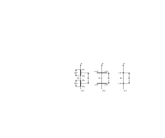
Figure 1: Identical Kerr-Newman-type sources on the symmetry axis: (a) BHs for $\sigma^{2}>0$; (b) hyperextreme sources if $\sigma\rightarrow i\sigma$ (or $\sigma^{2}<0$ ); (c) extreme BHs where $\sigma=0$.

where $\gamma^{H}$ is the value acquired by the metric function $\gamma$ over the horizon. Due to the fact that each thin rod representing the BH horizon in Fig. 1(a) contains the same length, without loss of generality, it is possible to calculate the Komar parameters by means of the values $H=\{-\sigma\leq z-R/2\leq\sigma,0\leq\varphi\leq 2\pi,\rho\rightarrow 0\}$, that define the upper BH. After using the Ernst potentials and metric functions derived in Ref. CCHV , the horizon mass $M_{H}$ and electromagnetic charge $Q_{H}+iB_{H}$ assume the form

$$M_{H}=M+\frac{2q_{o}(Q/M)P_{0}R(R^{2}-4\Delta)}{\Big{[}(R+2M)(R^{2}-4\Delta)-4\mathfrak{q}\delta\Big{]}^{2}+64\mathfrak{q}^{2}q_{o}^{2}(Q/M)^{2}}-M_{A}^{S},$$

$$Q_{H}+iB_{H}=Q+2\frac{P_{0}(q_{o}+ib_{o})+iQ\Big{(}\mathfrak{q}(R^{2}-4\Delta)+(R+2M)\big{[}\delta+2iq_{o}(Q/M)\big{]}\Big{)}}{(R+2M)(R^{2}-4\Delta)-4\mathfrak{q}\big{[}\delta+2iq_{o}(Q/M)\big{]}},$$ (13)

whereas the lower BH defines its corresponding horizon mass once is performed the change $q_{o}\rightarrow-q_{o}$ in Eq. (13), while its electromagnetic charge is $2Q-Q_{H}-iB_{H}$. In Ref. CCHV , the axis condition Eq. (7) has been combined together with Eq. (13) in order to derive two corotating electrically charged models; i.e., two binary systems of equal corotating Kerr-Newman BHs endowed with identical or opposite electric charges and separated by a massless strut, in which a DS binding the BHs does not exist since the absence of individual magnetic charges was also established. However, the contribution of the DS into the horizon mass might be considered if $B_{H}\neq 0$, where after setting $q_{o}=0$ in Eqs. (7) and (13) eventually one gets the result

$$\delta =\frac{2(R^{2}-4\Delta)\big{[}M\mathfrak{q}P_{0}+(R+2M)\tau\big{]}}{(R^{2}+2MR+4\mathfrak{q}^{2})P_{0}+8\mathfrak{q}\tau},\qquad b_{o}=-\frac{(R^{2}-4\Delta)\big{(}(2\mathfrak{q}Q_{H}-B_{H}R)P_{0}+4Q_{H}\tau\big{)}}{2\big{[}(R^{2}+2MR+4\mathfrak{q}^{2})P_{0}+8\mathfrak{q}\tau\big{]}},$$

$$\tau =\mathfrak{q}(Q_{H}^{2}-B_{H}^{2})-B_{H}Q_{H}(R+2M),\qquad Q=Q_{H},$$ (14)

that permits the description of a two-body system of corotating dyonic BHs connected by a DS, where the upper and lower constituents have electromagnetic charges equal to $Q_{H}+iB_{H}$ and $Q_{H}-iB_{H}$ respectively. Lengthy calculations eventually give us simple expressions for $M_{A}^{S}$, $\Phi_{E}^{H}$, and $\Omega$, namely

$$M_{A}^{S} =B_{H}\epsilon\Bigg{(}\frac{B_{H}\mathcal{L}-Q_{H}\mathcal{M}}{\mathcal{L}^{2}+\mathcal{M}^{2}}\Bigg{)},\qquad\Phi_{E}^{H}=\frac{Q_{H}(R+2\sigma)\mathcal{L}-2b_{0}\mathcal{M}}{\mathcal{L}^{2}+\mathcal{M}^{2}},\qquad\Omega=\frac{2\mathfrak{q}}{P_{0}}+\frac{\epsilon\mathcal{M}}{\mathcal{L}^{2}+\mathcal{M}^{2}},$$

$$\epsilon =\frac{P_{0}R(R^{2}-4\Delta)}{(R^{2}+2MR+4\mathfrak{q}^{2})P_{0}+8\mathfrak{q}\tau},\qquad\mathcal{L}=MR+2\Delta+(R+2M)\sigma,\qquad\mathcal{M}=\delta+\mathfrak{q}(R+2\sigma).$$ (15)

A second model emerges immediately from Eqs. (7) and (13) by doing first $Q=0$, to obtain

$$\delta =\frac{2\mathfrak{q}(R^{2}-4\Delta_{1})\big{[}MP_{0}-|\mathcal{Q}|^{2}(R+2M)\big{]}}{(R^{2}+2MR+4\mathfrak{q}^{2})P_{0}-8\mathfrak{q}^{2}|\mathcal{Q}|^{2}},\qquad\mathfrak{q}_{o}=\frac{\mathcal{Q}R(R^{2}-4\Delta_{1})P_{0}}{2\Big{[}(R^{2}+2MR+4\mathfrak{q}^{2})P_{0}-8\mathfrak{q}^{2}|\mathcal{Q}|^{2}\Big{]}},$$

$$\Delta_{1} =M^{2}-\mathfrak{q}^{2},\qquad\mathcal{Q}=Q_{H}+iB_{H},\qquad|\mathcal{Q}|^{2}=Q_{H}^{2}+B_{H}^{2},$$ (16)

thus having a binary system that contains opposite electromagnetic charges, where now it is possible to get

$$M_{A}^{S} =2B_{H}\Bigg{(}\frac{b_{o}\mathcal{N}-q_{o}\mathcal{M}}{\mathcal{N}^{2}+\mathcal{M}^{2}}-\frac{2\mathfrak{q}Q_{H}}{P_{0}}\Bigg{)},\qquad\Phi_{E}^{H}=2\frac{q_{o}\mathcal{N}-b_{o}\mathcal{M}}{\mathcal{N}^{2}+\mathcal{M}^{2}},\qquad\Omega=\frac{2\mathfrak{q}}{P_{0}}+\frac{2(q_{o}/Q_{H})\mathcal{M}}{\mathcal{N}^{2}+\mathcal{M}^{2}},$$

$$\mathcal{N} =MR+2\Delta_{1}+(R+2M)\sigma.$$ (17)

In both models, it should be observed the contribution of the DS via the magnetic charge $B_{H}$, where regardless of which one may be considered, the upper and lower dyonic BHs are equipped with a magnetic charge $B_{H}$ and $-B_{H}$ respectively. That each source carries a magnetic charge of opposite sign is one of the main characteristics of dyonic binary BH models joined by a DS, when the global monopolar magnetic charge has been eliminated from the configuration CCHV . It is important to comment that both dyonic BHs having a DS in between sources will satisfy the Smarr formula Eq. (11), in which their horizon mass is $M_{H}=M-M_{A}^{S}$.

II.1 Physical meaning of the DS into the horizon mass

At this point, we would like to discuss a little bit on some physical implications of $M_{A}^{S}$ within the Smarr formula. As has been recently proved by Clément and Gal’tsov Galtsov , the correctness of Tomimatsu’s formulas fails at the moment of including magnetic charges, due mainly to the fact that the horizon mass $M_{H}$ in Tomimatsu’s approach does not contain the extra component $M_{A}^{S}$. For that reason Tomimatsu’s expression for the horizon mass is determined by Tomi

$$M_{H}=\sigma+2\Omega J_{H}+\Phi^{H}_{E}Q_{H}+M_{A}^{S},$$ (18)

which looks different than the one displayed in Eq. (11). However, if we want to consider the contribution of the DS provided by the extra term $M_{A}^{S}$ into the horizon mass we need to include a constant in the magnetic potential, namely

$$A_{3new}=K_{0}+A_{3},$$ (19)

and it creates changes in the terms $M_{A}^{S}$ and $\Phi_{E}^{H}$ in the form

$$M_{Anew}^{S} =-\frac{1}{4\pi}\int_{H}(A_{3}^{{}^{\prime}}A_{3new})_{,z}d\varphi dz=M_{A}^{S}-K_{0}\Omega Q_{H},$$

$$\Phi_{Enew}^{H} =-A_{4}^{H}-\Omega A_{3new}^{H}=\Phi_{E}^{H}-K_{0}\Omega.$$ (20)

In order to explain how this constant might be used, and with the purpose to amend the discrepancy committed in CLLM1 ; CLLM2 ; CLM , we are going to appeal first to the results of the paper CLLM2 concerning to an oppositely electromagnetic charged two-body system of identical counterrotating BHs, where its thermodynamical properties were explicitly calculated; they read

$$M_{A}^{S} =B_{H}(B_{H}\phi^{H}-Q_{H}\Omega),\qquad\Phi_{E}^{H}=Q_{H}\phi^{H}-B_{H}\Omega,$$

$$\Omega =\frac{\mu}{2}\frac{(R+2\sigma)\sqrt{X-1}}{M[R+2\sigma-(R-2M)X]-\mu|\mathcal{Q}|^{2}},\qquad\phi^{H}=\frac{\mu}{2}\frac{R+2\sigma-(R-2M)X}{M[R+2\sigma-(R-2M)X]-\mu|\mathcal{Q}|^{2}},$$

$$\sigma =\sqrt{X\big{(}M^{2}-|\mathcal{Q}|^{2}\mu\big{)}+\frac{R^{2}}{4}(1-X)},\quad\mu=\frac{R-2M}{R+2M},$$ (21)

where $X$ is an auxiliary variable defined as

$$X=\frac{q_{o}^{2}+b_{o}^{2}}{(R/2-M)^{2}(Q_{H}^{2}+B_{H}^{2})},$$ (22)

which in the lack of rotation turns out to be equal to the unit. Due to the fact that the mass formula Eq. (11) now takes the form

$$M_{H}=M-M_{Anew}^{S}=\sigma+2\Omega J_{H}+\Phi^{H}_{Enew}Q_{H},$$ (23)

it is quite natural to deduce from Eqs. (20)-(21) that $K_{0}$ may be chosen as $K_{0}=-B_{H}$. Therefore, Eq. (23) is further simplified as follows

$$M_{H}\equiv M-B_{H}^{2}\phi^{H}=\sigma+2\Omega J_{H}+Q_{H}^{2}\phi^{H}.$$ (24)

The substitution of $\sigma$ from Eq. (21) into Eq. (24) allows us to obtain

$$X=1+\frac{4J_{H}^{2}}{\Big{[}M(R+2M)+|\mathcal{Q}|^{2}\Big{]}^{2}},$$ (25)

thus having the explicit form of $\sigma$

$$\sigma=\sqrt{M^{2}-\left(|\mathcal{Q}|^{2}+\frac{J_{H}^{2}\big{[}(R+2M)^{2}+4|\mathcal{Q}|^{2}\big{]}}{\big{[}M(R+2M)+|\mathcal{Q}|^{2}\big{]}^{2}}\right)\frac{R-2M}{R+2M}}.$$ (26)

Notice that there is a distinction between the horizon mass $M_{H}$ and the parameter $M$ as has been pointed out earlier by Clément and Gal’tsov Galtsov ; both are identical only whether the boundary term $M_{A}^{s}$ is killed due mainly to the fact that magnetic charges are not present. So, we have that in the limit $R\rightarrow\infty$, the horizon mass $M_{H}$ behaves as

$$M_{H} =\lim_{R\rightarrow\infty}\Big{[}M-B_{H}^{2}\phi^{H}\Big{]}=M-B_{H}^{2}\frac{M+\sigma}{(M+\sigma)^{2}+(J_{H}/M)^{2}},$$

$$\sigma =\sqrt{M^{2}-|\mathcal{Q}|^{2}-J_{H}^{2}/M^{2}},$$ (27)

recovering the expression for one isolated dyonic Kerr-Newman BH joined to a DS Galtsov . In this counterrotating sector, $J_{H}$ defines half of the total angular momentum of the system since it does not contain an extra contribution coming from the DS. On the other hand, the addition of the same constant $K_{0}=-B_{H}$ in the first corotating model with identical electric charges produces

$$M_{Anew}^{S} =B_{H}\Bigg{(}\frac{B_{H}\epsilon\mathcal{L}}{\mathcal{L}^{2}+\mathcal{M}^{2}}+\frac{2\mathfrak{q}Q_{H}}{P_{0}}\Bigg{)},\qquad\Phi_{Enew}^{H}=\frac{Q_{H}(R+2\sigma)\mathcal{L}-(2b_{0}-B_{H}\epsilon)\mathcal{M}}{\mathcal{L}^{2}+\mathcal{M}^{2}}+\frac{2\mathfrak{q}B_{H}}{P_{0}},$$

$$J_{H} =2M\mathfrak{q}-\frac{\delta}{2}-Q_{H}B_{H},$$ (28)

while its addition in the one carrying opposite electromagnetic charges generates the result

$$\qquad M_{Anew}^{S} =2B_{H}\Bigg{(}\frac{b_{o}\mathcal{N}}{\mathcal{N}^{2}+\mathcal{M}^{2}}-\frac{\mathfrak{q}Q_{H}}{P_{0}}\Bigg{)},\qquad\Phi_{Enew}^{H}=2\Bigg{(}\frac{q_{o}\mathcal{N}}{\mathcal{N}^{2}+\mathcal{M}^{2}}+\frac{\mathfrak{q}B_{H}}{P_{0}}\Bigg{)},$$

$$J_{H} =2M\mathfrak{q}-\frac{\delta}{2},$$ (29)

where it can be checked straightforwardly from these corotating models that Eq. (27) is recovered at an infinite separation distance, where $\mathfrak{q}=J_{H}/M$. The reader should further note that in the binary system with identical electric charges, $J_{H}$ equates the half of the total angular momentum only at large distances.

It should be mentioned here, that contrary to the statement provided by the authors in Ref. MankoCompean , there is no need to add any constant to the magnetic potential $A_{3}$ when a DR procedure has been applied to include the magnetic charge inside the Kerr-Newman solution. These authors MankoCompean have combined two approaches; the DR studied many years ago by Carter Carter and the addition of a constant in the magnetic potential $A_{3}$, with the objective to prove the correctness of Tomimatsu’s formulas in the presence of both electric and magnetic charges. However, their procedure cannot be correct since there was an error in such formulas that might lead to physical and mathematical inconsistencies. To prove the last statement on the no need of adding a constant in $A_{3}$, for simplicity and without loss of generality one might use once again the expressions of Eq. (21) after eliminating the magnetic charge, thus having

$$M_{A}^{S} =0,\quad\Phi_{E}^{H}=Q_{H}\phi^{H},$$

$$\Omega =\frac{\mu}{2}\frac{(R+2\sigma)\sqrt{X-1}}{M[R+2\sigma-(R-2M)X]-\mu Q_{H}^{2}},\qquad\phi^{H}=\frac{\mu}{2}\frac{R+2\sigma-(R-2M)X}{M[R+2\sigma-(R-2M)X]-\mu Q_{H}^{2}},$$

$$\sigma =\sqrt{X\big{(}M^{2}-Q_{H}^{2}\mu\big{)}+\frac{R^{2}}{4}(1-X)},$$ (30)

where now the mass formula Eq. (11) reads

$$M_{H}\equiv M=\sigma+2\Omega J_{H}+Q_{H}^{2}\phi^{H}.$$ (31)

Then we have that a DR procedure ($Q_{H}\rightarrow Q_{H}+iB_{H}$ and $Q_{H}^{2}\rightarrow Q_{H}^{2}+B_{H}^{2}$) extends the conventional mass formula by adding the magnetic charge as a fourth conserved parameter as follows

$$M_{H} =\sigma+2\Omega J_{H}+\Phi_{EL}^{H}Q_{H}+\Phi_{MAG}^{H}B_{H},$$

$$\Phi_{EL}^{H} =Q_{H}\phi^{H},\qquad\Phi_{MAG}^{H}=B_{H}\phi^{H},$$ (32)

with $\sigma$ having the same aspect as shown in Eq. (26), but the main distinction is that the parameter $M$ is now representing the horizon mass $M_{H}$. Hence, no DS exists in between BHs.

An heuristic point of view on the electromagnetic charge conservation is reached by killing first the magnetic charge with the condition Tomi

$$\frac{1}{4\pi}\int_{H}\omega A_{4,z}\,d\varphi dz=-\frac{1}{4\pi}\int_{H}A_{3,z}\,d\varphi dz=0,$$ (33)

which means that both potentials $A_{4}$ and $A_{3}$ will take the same value in the limits defining the BH horizon. Therefore, the DS joined to the BH is eliminated, and later on, the DR $\Phi\rightarrow\Phi e^{i\alpha}$ is applied, where the real and imaginary components of the new potential $\Phi e^{i\alpha}$ take the aspect

$$A_{4new}=A_{4}+\frac{B_{H}}{Q_{H}}A_{3}^{{}^{\prime}},\qquad A_{3new}^{{}^{\prime}}=-\frac{B_{H}}{Q_{H}}A_{4}+A_{3}^{{}^{\prime}},$$ (34)

whereby $\alpha=\arctan(B_{H}/Q_{H})$. Observe that the case $B_{H}=0$ recovers the original potential $\Phi$. Thus, we write the electric and magnetic charges as follows:

$$Q_{Hnew}=\frac{1}{4\pi}\int_{H}\omega A_{3new,z}^{{}^{\prime}}\,d\varphi dz,\qquad B_{Hnew}=\frac{1}{4\pi}\int_{H}\omega A_{4new,z}^{{}^{\prime}}\,d\varphi dz,$$ (35)

after the substitution of Eq. (34) into Eq. (35) it is possible to restore the contribution of the magnetic charge, namely

$$Q_{Hnew} =\frac{1}{4\pi}\int_{H}\omega\left(-\frac{B_{H}}{Q_{H}}A_{4}+A_{3}^{{}^{\prime}}\right)_{,z}\,d\varphi dz=Q_{H},$$

$$B_{Hnew} =\frac{1}{4\pi}\int_{H}\omega\left(A_{4}+\frac{B_{H}}{Q_{H}}A_{3}^{{}^{\prime}}\right)_{,z}\,d\varphi dz=Q_{H}\left(\frac{B_{H}}{Q_{H}}\right)=B_{H}.$$ (36)

The same idea depicted above can be worked out in order to prove that $M_{H}$ and $J_{H}$ are also conserved parameters under a DR, where we have that the new horizon mass and angular momentum assume the form

$$M_{Hnew} =M-M_{Anew}^{S}=M-M_{A}^{S}+\frac{B_{H}}{4\pi Q_{H}}\int_{H}(A_{4}A_{3})_{,z}d\varphi dz,$$

$$J_{Hnew} =-\frac{1}{8\pi}\int_{H}\omega\left[1+\frac{\omega\Psi_{,z}}{2}-\tilde{A}_{3}A_{3new,z}^{{}^{\prime}}\right]d\varphi dz-\frac{\omega^{H}M_{Anew}^{S}}{2},$$ (37)

where $M_{Hnew}=M_{H}=M$ and $J_{Hnew}=J_{H}$ once Eq. (33) is fulfilled to eliminate the DS. We now turn our attention to consider a DR in the solution CCHV in order to derive two corotating dyonic binary BH models with no DS in between.

II.2 Corotating dyonic BHs endowed with identical electromagnetic charges

An absence of magnetic charge ($B_{H}=0$) in Eq. (14) derives the following result

$$\delta =\frac{2\mathfrak{q}(R^{2}-4\Delta)\big{[}MP_{0}+Q_{H}^{2}(R+2M)\big{]}}{(R^{2}+2MR+4\mathfrak{q}^{2})P_{0}+8\mathfrak{q}^{2}Q_{H}^{2}},\qquad b_{o}=-\frac{\mathfrak{q}Q_{H}(R^{2}-4\Delta)\big{(}P_{0}+2Q_{H}^{2}\big{)}}{(R^{2}+2MR+4\mathfrak{q}^{2})P_{0}+8\mathfrak{q}^{2}Q_{H}^{2}},$$ (38)

where the extra term $M_{A}^{S}$ has been eliminated and for such a reason $M_{H}=M$. In this respect, the DR can be performed by doing only the following changes $Q_{H}\rightarrow Q_{H}+iB_{H}$ and $Q_{H}^{2}\rightarrow Q_{H}^{2}+B_{H}^{2}$ in the Ernst potentials on the symmetry axis given above in Eq. (4). The result is

$${\cal E}(0,z) =\frac{z^{2}-2(M+i\mathfrak{q})z+2\Delta_{o}-R^{2}/4-\sigma^{2}+i\delta}{z^{2}+2(M-i\mathfrak{q})z+2\Delta_{o}-R^{2}/4-\sigma^{2}-i\delta},\qquad\Phi(0,z)=\frac{2(\mathcal{Q}z+\mathfrak{q}_{o})}{z^{2}+2(M-i\mathfrak{q})z+2\Delta_{o}-R^{2}/4-\sigma^{2}-i\delta},$$ (39)

with

$$\delta =\frac{2\mathfrak{q}(R^{2}-4\Delta_{o})\big{[}MP_{0}+|\mathcal{Q}|^{2}(R+2M)\big{]}}{(R^{2}+2MR+4\mathfrak{q}^{2})P_{0}+8\mathfrak{q}^{2}|\mathcal{Q}|^{2}},\qquad\mathfrak{q}_{o}=-\frac{i\mathfrak{q}\mathcal{Q}(R^{2}-4\Delta_{o})\big{(}P_{0}+2|\mathcal{Q}|^{2}\big{)}}{(R^{2}+2MR+4\mathfrak{q}^{2})P_{0}+8\mathfrak{q}^{2}|\mathcal{Q}|^{2}},$$

$$\Delta_{o} =M^{2}-|\mathcal{Q}|^{2}-\mathfrak{q}^{2}.$$ (40)

It should be pointed out that this procedure has added the magnetic charge $B_{H}$ as a fourth conserved parameter into the solution, where now the electromagnetic charge obtainable from Eq. (13) is given by

$$Q_{H}+iB_{H}=Q_{H}+iB_{H}+2\frac{P_{0}(q_{o}+ib_{o})+i(Q_{H}+iB_{H})\Big{(}\mathfrak{q}(R^{2}-4\Delta_{o})+(R+2M)\delta\Big{)}}{(R+2M)(R^{2}-4\Delta_{o})-4\mathfrak{q}\delta},$$ (41)

which is identically satisfied by the set of variables expressed lines above in Eq. (40). Similar to the upper dyonic BH, the lower constituent contains the same electromagnetic charge $Q_{H}+iB_{H}$. Once we have incorporated the magnetic charge $B_{H}$, it follows that the Ernst potentials, Kinnersley potential $\Phi_{2}$, and metric functions read

$${\cal{E}} =\frac{\Lambda+\Gamma}{\Lambda-\Gamma},\quad\Phi=\frac{\chi}{\Lambda-\Gamma},\qquad\Phi_{2}=\frac{F}{\Lambda-\Gamma},\qquad f=\frac{|\Lambda|^{2}-|\Gamma|^{2}+|\chi|^{2}}{|\Lambda-\Gamma|^{2}},\qquad\omega=4\mathfrak{q}+\frac{{\rm{Im}}\left[(\Lambda-\Gamma)\overline{\mathcal{G}}-\chi\overline{\mathcal{I}}\right]}{|\Lambda|^{2}-|\Gamma|^{2}+|\chi|^{2}},$$

$$e^{2\gamma} =\frac{|\Lambda|^{2}-|\Gamma|^{2}+|\chi|^{2}}{64\sigma^{4}R^{4}\kappa_{o}^{2}r_{1}r_{2}r_{3}r_{4}},\qquad\Lambda=2\sigma^{2}\left[R^{2}\kappa_{o}(r_{1}+r_{2})(r_{3}+r_{4})+4a(r_{1}-r_{3})(r_{2}-r_{4})\right]$$

$$+2R^{2}\left[\kappa_{o}(2\Delta_{o}-\sigma^{2})-a\right](r_{1}-r_{2})(r_{3}-r_{4})+2iR\bigg{\{}\Big{(}2\mathfrak{q}{\rm Re}(s_{+})+{\rm Im}(p_{+})\Big{)}\Big{[}R(\mathfrak{r}_{1}-\mathfrak{r}_{2})(r_{3}-r_{4})$$

$$-2\sigma\big{(}\mathfrak{r}_{1}r_{4}-\mathfrak{r}_{2}r_{3}+4\sigma r_{3}r_{4}\big{)}\Big{]}+\mathfrak{q}\kappa_{o}\Big{[}r_{1}\big{(}R^{2}r_{3}-\kappa_{o}r_{4}\big{)}-r_{2}\big{(}\kappa_{o}r_{3}-R^{2}r_{4}\big{)}-8\sigma^{2}r_{3}r_{4}\Big{]}\bigg{\}},$$

$$\Gamma =4\sigma R\left(M\Gamma_{o}-b\chi_{+}\right),\qquad F=(4\mathfrak{q}+iz)\chi-i\mathcal{I},\qquad\chi=-4\sigma R\left(\mathcal{Q}\Gamma_{o}+2\mathbb{Q}\chi_{+}\right),\qquad\Gamma_{o}=R\chi_{-}-2\sigma\chi_{s}+2\chi_{1+},$$

$$\mathcal{G} =2z\Gamma+8\sigma^{2}\bigg{\{}R\Big{[}2\big{(}{\rm Re}(a)-2|\mathfrak{q}_{o}|^{2}\big{)}+|\mathcal{Q}|^{2}\kappa_{o}\Big{]}(r_{1}r_{2}-r_{3}r_{4})+2i\mathfrak{q}R^{2}\kappa_{o}(r_{2}r_{3}+r_{1}r_{4})+2i\Big{[}R{\rm Im}(a)+\overline{\mathcal{Q}}\xi_{0}-4\mathfrak{q}|\mathfrak{q}_{o}|^{2}\Big{]}$$

$$\times(r_{1}-r_{3})(r_{2}-r_{4})\bigg{\}}-4R^{2}\bigg{\{}\sigma\left[2a-(R-2\sigma)\Big{(}2(R+2i\mathfrak{q})s_{+}+p_{+}\Big{)}\right]+i\left(\overline{\mathcal{Q}}\xi_{o}+2i\mathfrak{q}_{o}\overline{\mathcal{Q}}\kappa_{o}-4\mathfrak{q}|\mathfrak{q}_{o}|^{2}\right)\bigg{\}}(r_{1}-r_{2})(r_{3}-r_{4})$$

$$+2\sigma R^{2}\bigg{\{}4\Big{(}2\kappa_{o}\Delta_{o}-{\rm Re}(a)\Big{)}r_{4}+\big{[}|\mathcal{Q}|^{2}\kappa_{o}+4|\mathfrak{q}_{o}|^{2}\big{]}(r_{3}+r_{4})\bigg{\}}(r_{1}-r_{2})$$

$$+2\sigma R^{2}\bigg{\{}4\Big{(}2\kappa_{o}\Delta_{o}-{\rm Re}(a)\Big{)}r_{2}+\big{[}|\mathcal{Q}|^{2}\kappa_{o}+4|\mathfrak{q}_{o}|^{2}\big{]}(r_{1}+r_{2})\bigg{\}}(r_{3}-r_{4})+4M\sigma R\big{(}\kappa_{o}\chi_{+}+2R\chi_{1-}+4\sigma^{2}\chi_{p}\big{)}$$

$$-4b\sigma R(R\chi_{-}+2\sigma\chi_{s})-8\sigma R(\mathcal{Q}b+2M\mathbb{Q})\Big{[}2\overline{\mathfrak{q}}_{o}\big{(}\mathfrak{r}_{1}-\mathfrak{r}_{2}+\mathfrak{r}_{3}-\mathfrak{r}_{4}\big{)}+\overline{\mathcal{Q}}\kappa_{o}(r_{1}-r_{2}-r_{3}+r_{4})\Big{]},$$

$$\mathcal{I} =A\Big{[}4\sigma^{2}(r_{1}-r_{3})(r_{2}-r_{4})-R^{2}(r_{1}-r_{2})(r_{3}-r_{4})\Big{]}+R\kappa_{-}\Big{[}B_{+}\kappa_{o}r_{1}-B_{-}R\mathfrak{r}_{2}\Big{]}r_{4}-R\kappa_{+}\Big{[}B_{+}R\mathfrak{r}_{1}-B_{-}\kappa_{o}r_{2}\Big{]}r_{3}$$

$$-16\sigma^{2}R\bigg{\{}\Big{[}M(R+2\sigma)(\kappa_{+}+2\mathcal{Q}R)-B_{+}\mathfrak{q}_{o}\Big{]}r_{3}r_{4}-R\kappa_{o}(2M\mathbb{Q}+\mathcal{Q}b)\bigg{\}}+8\mathbb{Q}\sigma R(\chi_{1+}+\sigma\chi_{s})$$

$$+2\sigma R\Big{[}\mathcal{Q}\big{(}2R^{2}-8\Delta_{o}+\kappa_{o}\big{)}+8i\mathfrak{q}\mathbb{Q}\Big{]}\chi_{+}+12\sigma R^{2}\mathbb{Q}\chi_{-}+8\mathcal{Q}\sigma R(R\chi_{1-}+2\sigma\chi_{p}),$$

$$\chi_{\pm} =s_{+}\mathfrak{r}_{1}-s_{-}\mathfrak{r}_{2}\pm(\bar{s}_{-}\mathfrak{r}_{3}-\bar{s}_{+}\mathfrak{r}_{4}),\quad\chi_{1\pm}=p_{+}\mathfrak{r}_{1}+p_{-}\mathfrak{r}_{2}\pm(\bar{p}_{-}\mathfrak{r}_{3}+\bar{p}_{+}\mathfrak{r}_{4}),\quad\chi_{s}=s_{+}\mathfrak{r}_{1}+s_{-}\mathfrak{r}_{2}+\bar{s}_{-}\mathfrak{r}_{3}+\bar{s}_{+}\mathfrak{r}_{4},$$

$$\chi_{p} =p_{+}\mathfrak{r}_{1}-p_{-}\mathfrak{r}_{2}+\bar{p}_{-}\mathfrak{r}_{3}-\bar{p}_{+}\mathfrak{r}_{4},\quad a=(R+2i\mathfrak{q})p_{+}-s_{+}\big{[}s_{+}-(R+2i\mathfrak{q})^{2}\big{]},\quad b=i(\delta-4M\mathfrak{q}),\quad\kappa_{o}=R^{2}-4\sigma^{2},$$

$$A =4M\Big{[}\big{(}2\mathbb{Q}+\mathcal{Q}(R-2\sigma)\big{)}s_{+}+2\mathcal{Q}p_{+}\Big{]}+B_{+}\Big{[}\mathcal{Q}\big{(}R^{2}-4\Delta_{o}\big{)}-2(R+2i\mathfrak{q})\mathfrak{q}_{o}\Big{]},\quad\kappa_{\pm}=2\mathfrak{q}_{o}-\mathcal{Q}(R\pm 2\sigma),$$

$$B_{\pm} =\Big{[}Rs_{\pm}\pm p_{\pm}+2\mathcal{Q}\big{(}2\overline{\mathfrak{q}}_{o}+\overline{\mathcal{Q}}(R\pm 2\sigma)\big{)}\Big{]}/M,\quad p_{\pm}=-\sigma(R^{2}-4\Delta_{o})\pm i\big{[}2M\delta+4i\mathcal{Q}\overline{\mathfrak{q}}_{o}-(R+2i\mathfrak{q}){\rm Im}(s_{\pm})\big{]},$$

$$s_{\pm} =2\Delta_{o}\pm\sigma R+i\mathfrak{q}(R\pm 2\sigma),\quad\xi_{o}=4\mathcal{Q}\Big{[}M\delta-2i\mathfrak{q}_{o}\overline{\mathcal{Q}}+\mathfrak{q}(\Delta_{o}-\sigma^{2})\Big{]}+(2i\mathfrak{q}_{o}-\mathfrak{q}\mathcal{Q})(R^{2}-4\Delta_{o}),\quad\mathbb{Q}=\mathfrak{q}_{o}+2i\mathfrak{q}\mathcal{Q},$$

$$\mathfrak{r}_{1,4} =(R-2\sigma)r_{1,4},\quad\mathfrak{r}_{2,3}=(R+2\sigma)r_{2,3},$$ (42)

where the half-length parameter defining the BH horizon can be written as

$$\sigma=\sqrt{\Delta_{o}-\frac{4|\mathfrak{q}_{o}|^{2}-\delta^{2}}{R^{2}-4\Delta_{o}}},$$ (43)

which explicitly is

$$\sigma =\sqrt{\Delta_{o}+\frac{4\mathfrak{q}^{2}(R^{2}-4\Delta_{o})\Big{[}\big{[}MP_{0}+|\mathcal{Q}|^{2}(R+2M)\big{]}^{2}-|\mathcal{Q}|^{2}(P_{0}+2|\mathcal{Q}|^{2})^{2}\Big{]}}{\big{[}(R^{2}+2MR+4\mathfrak{q}^{2})P_{0}+8\mathfrak{q}^{2}|\mathcal{Q}|^{2}\big{]}^{2}}}.$$ (44)

In this case the components of the extended mass formula Eq. (32), $\Omega$ and $\phi^{H}$ are given by

$$\Omega =\frac{2\mathfrak{q}}{P_{0}}+\frac{P_{0}R(R^{2}-4\Delta_{o})}{(R^{2}+2MR+4\mathfrak{q}^{2})P_{0}+8\mathfrak{q}^{2}|\mathcal{Q}|^{2}}\Bigg{(}\frac{\mathcal{M}}{\mathcal{L}_{o}^{2}+\mathcal{M}^{2}}\Bigg{)},\qquad\phi^{H}=\frac{(R+2\sigma)\mathcal{L}_{o}-2(b_{o}/Q_{H})\mathcal{M}}{\mathcal{L}^{2}_{o}+\mathcal{M}^{2}},$$

$$\mathcal{L}_{o} =MR+2\Delta_{o}+(R+2M)\sigma,$$ (45)

and their combination with Eq.(̇44) defines the angular momentum from Eq. (32), to obtain

$$J_{H}=2M\mathfrak{q}-\frac{\mathfrak{q}(R^{2}-4\Delta_{o})\big{[}MP_{0}+|\mathcal{Q}|^{2}(R+2M)\big{]}}{(R^{2}+2MR+4\mathfrak{q}^{2})P_{0}+8\mathfrak{q}^{2}|\mathcal{Q}|^{2}},$$ (46)

which is nothing less than half of the total angular momentum;i.e., $2M\mathfrak{q}-\delta/2$. In addition, we have that the area of the horizon $S$ and surface gravity $\kappa$ are expressed as

$$\frac{S}{4\pi}=\frac{\sigma}{\kappa}=\frac{\mathcal{L}_{o}^{2}+\mathcal{M}^{2}}{R(R+2\sigma)}.$$ (47)

The conical singularity (or strut) along the line keeping apart the BHs from overlapping presents an angular deficit $\Delta\varphi=-8\pi\mathcal{\mathcal{F}}$, where the interaction force $\mathcal{F}$ is computed with the aid of the formula $\mathcal{F}=(e^{-\gamma_{s}}-1)/4$ Israel ; Weinstein , being $\gamma_{s}$ the constant value for the metric function $\gamma$ in the axis region in between sources. The result is

$$\mathcal{F} =\frac{\big{[}(M^{2}-|\mathcal{Q}|^{2})P_{0}^{2}-4\mathfrak{q}^{2}|\mathcal{Q}|^{4}\big{]}(P_{0}-8\mathfrak{q}^{2})-16\mathfrak{q}^{2}|\mathcal{Q}|^{2}\Big{[}\big{(}M(R+2M)-|\mathcal{Q}|^{2}\big{)}P_{0}-|\mathcal{Q}|^{4}\Big{]}}{(R^{2}-4\Delta_{o})P_{0}^{3}}.$$ (48)

The strut is massless because does not contribute to the total gravitational energy of the system. The force $\mathcal{F}\rightarrow 0$ at $R\rightarrow\infty$, where Eqs. (44) and (46) permit us to recover the expression $\sigma=\sqrt{M_{H}^{2}-|\mathcal{Q}|^{2}-J_{H}^{2}/M_{H}^{2}}$ defining an isolated dyonic BH free of monopolar sources. Moreover, not taking into account large separation distances, the lack of a conical singularity is achieved when $\mathcal{F}=0$, and due to the fact that the numerator of $\mathcal{F}$ is a bicubic equation in the variable $\mathfrak{q}$, in principle this task can be done analytically. This matter clearly deserves further research in order to understand better the presence of ring singularities off the axis or other pathologies like closed time-like curves.

We end this subsection, by mentioning that the aforementioned expression of the force Eq. (48) will contain a different aspect if the DS is taken into account in the solution.

II.3 Corotating dyonic BHs endowed with opposite electromagnetic charges

The second charged model arises after setting $B_{H}=0$ in Eq. (16), thus having

$$\delta =\frac{2\mathfrak{q}(R^{2}-4\Delta_{1})\big{[}MP_{0}-Q_{H}^{2}(R+2M)\big{]}}{(R^{2}+2MR+4\mathfrak{q}^{2})P_{0}-8\mathfrak{q}^{2}Q_{H}^{2}},\qquad q_{o}=\frac{Q_{H}R(R^{2}-4\Delta_{1})P_{0}}{2\Big{[}(R^{2}+2MR+4\mathfrak{q}^{2})P_{0}-8\mathfrak{q}^{2}Q_{H}^{2}\Big{]}},$$ (49)

where now each BH contains an opposite electric charge. So, in this case the Ernst potentials on the symmetry axis after performing the DR are written as

$${\cal E}(0,z) =\frac{z^{2}-2(M+i\mathfrak{q})z+2\Delta_{1}-R^{2}/4-\sigma^{2}+i\delta}{z^{2}+2(M-i\mathfrak{q})z+2\Delta_{1}-R^{2}/4-\sigma^{2}-i\delta},\qquad\Phi(0,z)=\frac{2\mathfrak{q}_{o}}{z^{2}+2(M-i\mathfrak{q})z+2\Delta_{1}-R^{2}/4-\sigma^{2}-i\delta},$$ (50)

with $\delta$ and $q_{o}$ having the same aspect as in Eq. (16), but now $M=M_{H}$ since $M_{A}^{S}=0$. The electromagnetic charge derived from Eq. (13) and satisfied by Eq. (16) reduces to

$$Q_{H}+iB_{H}=\frac{2(q_{o}+ib_{o})P_{0}}{(R+2M)(R^{2}-4\Delta_{1})-4\mathfrak{q}\delta}.$$ (51)

It is worthwhile to mention, that the lower dyonic BH is endowed with opposite electromagnetic charge; i.e.,$-Q_{H}-iB_{H}$. Then, the Ernst and Kinnersley potentials, as well as the metric functions, have now the form

$${\cal{E}} =\frac{\Lambda+\Gamma}{\Lambda-\Gamma},\qquad\Phi=\frac{\chi}{\Lambda-\Gamma},\qquad\Phi_{2}=\frac{F}{\Lambda-\Gamma},\qquad f=\frac{|\Lambda|^{2}-|\Gamma|^{2}+|\chi|^{2}}{|\Lambda-\Gamma|^{2}},\qquad\omega=4\mathfrak{q}+\frac{{\rm{Im}}\left[(\Lambda-\Gamma)\overline{\mathcal{G}}-\chi\overline{\mathcal{I}}\right]}{|\Lambda|^{2}-|\Gamma|^{2}+|\chi|^{2}},$$

$$e^{2\gamma} =\frac{|\Lambda|^{2}-|\Gamma|^{2}+|\chi|^{2}}{64\sigma^{4}R^{4}\kappa_{o}^{2}r_{1}r_{2}r_{3}r_{4}},\qquad\Lambda=2\sigma^{2}\left[R^{2}\kappa_{o}(r_{1}+r_{2})(r_{3}+r_{4})+4a(r_{1}-r_{3})(r_{2}-r_{4})\right]$$

$$+2R^{2}\left[\kappa_{o}(2\Delta_{1}-\sigma^{2})-a\right](r_{1}-r_{2})(r_{3}-r_{4})+2iR\bigg{\{}\Big{(}2\mathfrak{q}{\rm Re}(s_{+})+{\rm Im}(p_{+})\Big{)}\Big{[}R(\mathfrak{r}_{1}-\mathfrak{r}_{2})(r_{3}-r_{4})$$

$$-2\sigma\big{(}\mathfrak{r}_{1}r_{4}-\mathfrak{r}_{2}r_{3}+4\sigma r_{3}r_{4}\big{)}\Big{]}+\mathfrak{q}\kappa_{o}\Big{[}r_{1}\big{(}R^{2}r_{3}-\kappa_{o}r_{4}\big{)}-r_{2}\big{(}\kappa_{o}r_{3}-R^{2}r_{4}\big{)}-8\sigma^{2}r_{3}r_{4}\Big{]}\bigg{\}},$$

$$\Gamma =4\sigma R\left(M\Gamma_{o}-b\chi_{+}\right),\quad F=(4\mathfrak{q}+iz)\chi-i\mathcal{I},\quad\chi=-8\sigma R\mathfrak{q}_{o}\chi_{+},\quad\Gamma_{o}=R\chi_{-}-2\sigma\chi_{s}+2\chi_{1+},$$

$$\mathcal{G} =2z\Gamma+8\sigma^{2}\Bigg{\{}2R\big{(}{\rm Re}(a)-2|\mathfrak{q}_{o}|^{2}\big{)}(r_{1}r_{2}-r_{3}r_{4})+2i\mathfrak{q}R^{2}\kappa_{o}(r_{2}r_{3}+r_{1}r_{4})+2i\Big{[}R{\rm Im}(a)-4\mathfrak{q}|\mathfrak{q}_{o}|^{2}\Big{]}(r_{1}-r_{3})(r_{2}-r_{4})$$

$$-4R^{2}\bigg{(}\sigma\left[2a-(R-2\sigma)\Big{(}2(R+2i\mathfrak{q})s_{+}+p_{+}\Big{)}\right]-4i\mathfrak{q}|\mathfrak{q}_{o}|^{2}\bigg{)}(r_{1}-r_{2})(r_{3}-r_{4})\Bigg{\}}$$

$$+8\sigma R^{2}\Big{[}\big{(}2\kappa_{o}\Delta_{1}-{\rm Re}(a)\big{)}r_{4}+|\mathfrak{q}_{o}|^{2}(r_{3}+r_{4})\Big{]}(r_{1}-r_{2})+8\sigma R^{2}\Big{[}\big{(}2\kappa_{o}\Delta_{1}-{\rm Re}(a)\big{)}r_{2}+|\mathfrak{q}_{o}|^{2}(r_{1}+r_{2})\Big{]}(r_{3}-r_{4})$$

$$+4\sigma R\bigg{\{}M\Big{[}\kappa_{o}\chi_{+}+2R\chi_{1-}+4\sigma\chi_{p}-8|\mathfrak{q}_{o}|^{2}(\mathfrak{r}_{1}-\mathfrak{r}_{2}+\mathfrak{r}_{3}-\mathfrak{r}_{4})\Big{]}-b\big{(}R\chi_{-}+2\sigma\chi_{s}\big{)}\bigg{\}},$$

$$\mathcal{I} =4\mathfrak{q}_{o}\bigg{\{}A\Big{[}4\sigma^{2}(r_{1}-r_{3})(r_{2}-r_{4})-R^{2}(r_{1}-r_{2})(r_{3}-r_{4})\Big{]}+R\Big{[}B_{+}\Big{(}(R+2\sigma)r_{4}-Rr_{3}\Big{)}\mathfrak{r}_{1}+B_{-}\Big{(}(R-2\sigma)r_{3}-Rr_{4}\Big{)}\mathfrak{r}_{2}\Big{]}$$

$$-8\sigma^{2}R\Big{[}\Big{(}M(R+2\sigma)-B_{+}\Big{)}r_{3}r_{4}-MRk_{o}\Big{]}+2\sigma R(\chi_{1+}+\sigma\chi_{s})+4i\mathfrak{q}\sigma R\chi_{+}+3\sigma R^{2}\chi_{-}\bigg{\}},$$

$$\chi_{\pm} =s_{+}\mathfrak{r}_{1}-s_{-}\mathfrak{r}_{2}\pm(\bar{s}_{-}\mathfrak{r}_{3}-\bar{s}_{+}\mathfrak{r}_{4}),\quad\chi_{1\pm}=p_{+}\mathfrak{r}_{1}+p_{-}\mathfrak{r}_{2}\pm(\bar{p}_{-}\mathfrak{r}_{3}+\bar{p}_{+}\mathfrak{r}_{4}),\quad\chi_{s}=s_{+}\mathfrak{r}_{1}+s_{-}\mathfrak{r}_{2}+\bar{s}_{-}\mathfrak{r}_{3}+\bar{s}_{+}\mathfrak{r}_{4},$$

$$\chi_{p} =p_{+}\mathfrak{r}_{1}-p_{-}\mathfrak{r}_{2}+\bar{p}_{-}\mathfrak{r}_{3}-\bar{p}_{+}\mathfrak{r}_{4},\quad a=(R+2i\mathfrak{q})p_{+}-s_{+}\big{[}s_{+}-(R+2i\mathfrak{q})^{2}\big{]},\quad b=i(\delta-4M\mathfrak{q}),\quad\kappa_{o}=R^{2}-4\sigma^{2},$$

$$A =2Ms_{+}-(R+2i\mathfrak{q})B_{+},\quad B_{\pm}=M(R\pm 2\sigma)+i\delta,\quad p_{\pm}=-\sigma(R^{2}-4\Delta_{1})\pm i\big{[}2M\delta-(R+2i\mathfrak{q}){\rm Im}(s_{\pm})\big{]},$$

$$s_{\pm} =2\Delta_{1}\pm\sigma R+i\mathfrak{q}(R\pm 2\sigma),\quad\mathfrak{r}_{1,4}=(R-2\sigma)r_{1,4},\quad\mathfrak{r}_{2,3}=(R+2\sigma)r_{2,3},\quad$$ (52)

with $\sigma$ having now the aspect

$$\sigma =\sqrt{\Delta_{1}+\frac{(R^{2}-4\Delta_{1})\Big{[}\big{[}2\mathfrak{q}\big{(}MP_{0}-|\mathcal{Q}|^{2}(R+2M)\big{)}\big{]}^{2}-(|\mathcal{Q}|RP_{0})^{2}\Big{]}}{\big{[}(R^{2}+2MR+4\mathfrak{q}^{2})P_{0}-8\mathfrak{q}^{2}|\mathcal{Q}|^{2}\big{]}^{2}}}.$$ (53)

On the other hand, the thermodynamical properties of the extended Smarr formula Eq. (32) become

$$\Omega =\frac{2\mathfrak{q}}{P_{0}}+\phi^{H},\qquad\phi^{H}=\frac{2(q_{o}/Q_{H})\mathcal{N}}{\mathcal{N}^{2}+\mathcal{M}^{2}},\qquad\frac{S}{4\pi}=\frac{\sigma}{\kappa}=\frac{\mathcal{N}^{2}+\mathcal{M}^{2}}{R(R+2\sigma)},$$ (54)

where they define the angular momentum of the horizon in the way

$$J_{H}=2M\mathfrak{q}-\frac{\mathfrak{q}(R^{2}-4\Delta_{1})\big{[}MP_{0}-|\mathcal{Q}|^{2}(R+2M)\big{]}}{(R^{2}+2MR+4\mathfrak{q}^{2})P_{0}-8\mathfrak{q}^{2}|\mathcal{Q}|^{2}}.$$ (55)

Moreover, it is not difficult to show that the interaction force is given by

$$\mathcal{F}=\frac{\big{(}M^{2}P_{0}^{2}-4\mathfrak{q}^{2}|\mathcal{Q}|^{4}\big{)}(P_{0}-8\mathfrak{q}^{2})+|\mathcal{Q}|^{2}\big{[}R^{2}P_{0}-4\mathfrak{q}^{2}(R^{2}-4\Delta_{1})\big{]}P_{0}}{(R^{2}-4\Delta_{1})P_{0}^{3}},$$ (56)

It is noteworthy that if the DS is not absent in the solution, the interaction force looks the same as in Eq. (56), nonetheless $M\neq M_{H}$. In the same manner as in the first case, the strut may be removed by solving another bicubic equation in terms of $\mathfrak{q}$. To finalize the section, we mention that if $B_{H}=0$, all the physical and thermodynamical features in both models are reduced to those ones defining corotating binary systems of identical Kerr-Newman BHs CCHV .

III Concluding remarks

Following Carter’s approach Carter , we have been able to apply a DR in two identical corotating Kerr-Newman binary BH models recently studied in CCHV with the purpose to add individual magnetic charges to each BH. Therefore, each corotating BH is endowed with identical/opposite electromagnetic charge in the first/second configuration and satisfying a generalized Smarr formula for dyonic BHs. These models containing a conical singularity in between sources, are well represented by five physical arbitrary parameters $\{M_{H},J_{H},Q_{H},B_{H},R\}$ and they will be useful to provide further analytical studies of some astrophysical phenomena like geodesics, quasinormal modes or lensing and shadow effects in the context of binary BHs, among others. It is worth remarking that the DR approach describes configurations free of DS joined to the BHs. On the other hand, we have also shown in both corotating dyonic models that the mass $M_{H}$, angular momentum $J_{H}$, and electromagnetic charge $Q_{H}+iB_{H}$ are conserved parameters under DR and there is no necessity to add a gauge in the magnetic potential $A_{3}$ as has been claimed in MankoCompean . On the contrary, the addition of a gauge is only needed when the contribution of the DS into the horizon mass $M_{H}$ is introduced in order to balance each dyonic BH. In all the scenarios examined in this work, this gauge is a constant of value $K_{0}=-B_{H}$ that leads us to the correct description of an isolated BH joined to a DS previously studied by Clément and Gal’tsov Galtsov .

We would like to point out that the metric for the extreme limit case $(\sigma=0)$ of corotating dyonic BHs has not been considered here since it can be easily derived from the formulas given in CCHV , where both electrically charged configurations were well defined. In fact, it should be mentioned that both dyonic configurations satisfy the Gabach-Clement identity Maria for extreme BHs with struts, namely

$$\sqrt{1+4\mathcal{F}_{ext}}=\frac{\sqrt{(8\pi J_{H})^{2}+(4\pi Q_{H}^{2}+4\pi B_{H}^{2})^{2}}}{S_{ext}},$$ (57)

where $S_{ext}$ and $\mathcal{F}_{ext}$ define the horizon area and the force in the extreme case, respectively. Due to the fact that the expression of the force contains the same aspect in both extreme and non-extreme configurations, because it does not depend on $\sigma$. For instance, in the identically electromagnetic charged model, we have that

$$S_{ext}=4\pi\frac{(MR+2\Delta_{o})^{2}+(\delta+\mathfrak{q}R)^{2}}{R^{2}},$$ (58)

and the substitution of Eqs. (46), (48), and (58) into Eq. (57) yields

$$\Delta_{o}+\frac{4\mathfrak{q}^{2}(R^{2}-4\Delta_{o})\Big{[}\big{[}MP_{0}+|\mathcal{Q}|^{2}(R+2M)\big{]}^{2}-|\mathcal{Q}|^{2}(P_{0}+2|\mathcal{Q}|^{2})^{2}\Big{]}}{\big{[}(R^{2}+2MR+4\mathfrak{q}^{2})P_{0}+8\mathfrak{q}^{2}|\mathcal{Q}|^{2}\big{]}^{2}}=0,$$ (59)

which is exactly the condition $\sigma=0$ on Eq. (44) for extreme dyonic BHs. Furthermore, one may proceed in the same manner for the oppositely dyonic charged configuration in order to derive once again the expression that arises from the condition $\sigma=0$ imposed on Eq. (53).

References

References

• (1) C. Misner, K. Thorne, and J. Wheeler, Gravitation, W. H. Freeman and Company (1973).
• (2) W. Israel, Event Horizons in Static Vacuum spacetimes, Phys. Rev. 164 (1967) 1776; W. Israel, Event Horizons in static electrovac spacetimes, Commun. Math Phys 8 (1968) 245.
• (3) B. Carter, Axisymmetric Black Hole Has Only Two degrees of Freedom, Phys. Rev. Lett. 26 (1971) 331; D. C. Robinson, Uniqueness of the Kerr Black Hole, Phys. Rev. Lett. 34 (1975) 905.
• (4) P. O. Mazur, Proof of uniqueness of the Kerr-Newman black hole solotion, J. Phys. A 15 (1982) 3173.
• (5) E. Newman, E. Couch, K. Chinnapared, A. Exton, A. Prakash, and R. Torrence, Metric of a rotating charged mass, J. Math. Phys. 6 (1965) 918.
• (6) J. D. Bekenstein, Black Holes: Classical Properties, Thermodynamics and Heuristic Quantization, arXiv:gr.qc/9808028v3.
• (7) B. Carter, Republication of: Black hole equilibrium states Part II. General theory of stationary black hole states, Gen. Relativ. Gravit. 42 (2010) 653.
• (8) J. S. Schwinger, A Magnetic Model of Matter, Science 165 (1969) 757.
• (9) L. Smarr, Mass formula for Kerr black holes, Phys. Rev. Lett. 30 (1973) 71.
• (10) A. Tomimatsu, Equilibrium of two rotating charged black holes and the Dirac string, Prog. Theor. Phys. 72 (1984) 73.
• (11) A. Komar, Covariant conservation laws in general relativity, Phys. Rev. 113 (1959) 934.
• (12) Gérard Clément and Dmitri Gal’tsov, On the Smarr formula for rotating dyonic black holes, Phys. Lett. B 773 (2017) 290.
• (13) I. Cabrera-Munguia, Claus Lämmerzahl, L. A. López, and Alfredo Macías, Opposite charged two-body system of identical counterrotating black holes, Phys. Rev. D 88 (2013) 084062.
• (14) I. Cabrera-Munguia, Claus Lämmerzahl, L. A. López, and Alfredo Macías, Generalized black diholes, Phys. Rev. D 90 (2014) 024013.
• (15) I. Cabrera-Munguia, Claus Lämmerzahl, and Alfredo Macías, Asymmetric black dyonic holes, Phys. Lett. B 743 (2015) 357.
• (16) R. Bach and H. Weyl, Neue Lösungen der Einsteinschen Gravitationsleichungen, Math. Z. 13 (1922) 134.
• (17) W. Israel, Line sources in general relativity, Phys. Rev. D 15 (1977) 935.
• (18) I. Cabrera-Munguia, Etevaldo dos Santos Costa Filho, Héctor H. Hernández, and David Vázquez-Valdez, Corotating binary systems of identical Kerr-Newman black holes, Phys. Lett. B 811 (2020) 135917.
• (19) V. S. Manko and H. García-Compean, Smarr formula for black holes endowed with both electric and magnetic charges, Class. Quantum Grav. 35 (2018) 064001.
• (20) F. J. Ernst, New formulation of the axially symmetric gravitational field problem. II, Phys. Rev. 168 (1968) 1415.
• (21) A. Papapetrou, A static solution of the equations of the gravitational field for an arbitrary, charge distribution, Proc. Roy. Irish Acad. A 51 (1947) 191.
• (22) N. R. Sibgatullin, Oscillations and Waves in Strong Gravitational and Electromagnetic Fields, Springer-Verlag, Berlin, 1991.
• (23) C. Hoenselaers and Z. Perjés, Multipole moments of axisymmetric electrovacuum spacetimes, Class. Quantum Grav. 7 (1990) 1819.
• (24) T. P. Sotiriou and T. A. Apostolatos, Corrections and comments on the multipole moments of axisymmetric spacetimes, Class. Quantum Grav. 21 (2004) 5727.
• (25) W. Simon, The multipole expansion of stationary Einstein-Maxwell fields, J. Math. Phys. (N. Y.) 25 (1984) 1035.
• (26) W. Kinnersley, Symmetries of the stationary Einstein-Maxwell field equations. I, J. Math. Phys. (N.Y.) 18 (1977) 1529.
• (27) B. Carter, in General Relativity, an Einstein Centenary Survey, edited by S. W. Hawking and W. Israel (Cambridge University Press, Cambridge, 1979), p. 294.
• (28) G. Weinstein, On rotating black holes in equilibrium in general relativity, Commun. Pure Appl. Math. 43 (1990) 903.
• (29) M. E. Gabach Clement, Bounds of the force between black holes, Class. Quantum Grav. 29 (2012) 165008.