Backpropagation through Signal Temporal Logic Specifications: Infusing Logical Structure into Gradient-Based Methods

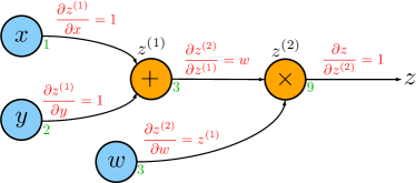
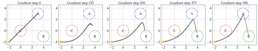
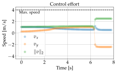
Abstract

This paper presents a technique, named stlcg, to compute the quantitative semantics of Signal Temporal Logic (STL) formulas using computation graphs. stlcg provides a platform which enables the incorporation of logical specifications into robotics problems that benefit from gradient-based solutions. Specifically, STL is a powerful and expressive formal language that can specify spatial and temporal properties of signals generated by both continuous and hybrid systems. The quantitative semantics of STL provide a robustness metric, i.e., how much a signal satisfies or violates an STL specification. In this work, we devise a systematic methodology for translating STL robustness formulas into computation graphs. With this representation, and by leveraging off-the-shelf automatic differentiation tools, we are able to efficiently backpropagate through STL robustness formulas and hence enable a natural and easy-to-use integration of STL specifications with many gradient-based approaches used in robotics. Through a number of examples stemming from various robotics applications, we demonstrate that stlcg is versatile, computationally efficient, and capable of incorporating human-domain knowledge into the problem formulation.

1 Introduction

There are rules or spatio-temporal constraints that govern how a system should operate. Depending on the application, a system could refer to a robotic system (e.g., autonomous car or drone), or components within an autonomy stack (e.g., controller, monitor, or predictor). Such rules or constraints can be explicitly known based on the problem definition or stem from human domain knowledge. For instance, road rules dictate how drivers on the road should behave, or search-and-rescue protocols prescribe how drones should survey multiple regions of a forest. Knowledge of such rules is not only critical for successful deployment and is also a useful form of inductive bias when designing such a system.

A common approach to translating rules or spatio-temporal constraints expressed as natural language into a mathematical representation is to use a logic-based formal language, a mathematical language that consists of logical operators and a grammar describing how to systematically combine logical operators in order to build more complex logical expressions. While the choice of a logic language can be tailored towards the application, one of the most common logic languages used in robotics is Linear Temporal Logic (LTL) (Pnueli, 1977; Baier and Katoen, 2008; Kress-Gazit et al., 2018; Wongpiromsarn et al., 2011; Fainekos et al., 2008), a temporal logic language that can describe and specify temporal properties of a sequence of discrete states (e.g., the traffic light will always eventually turn green). For example, Finucane et al. (2010) uses LTL to synthesize a “fire-fighting” robot planner that patrols a “burning” house to rescue humans and remove hazardous items. Part of the popularity of LTL is rooted in the fact that many planning problems with LTL constraints, if formulated in a certain way, can be cast into an automaton for which there are well-studied and tractable methods to synthesize a planner satisfying the LTL specifications (Baier and Katoen, 2008). However, the discrete nature of LTL makes its usage limited to high-level planners and faces scalability issues when considering high-dimensional, continuous, or nonlinear systems. Importantly, LTL is incompatible with gradient-based methods since LTL operates on discrete states.

Recently, Signal Temporal Logic (STL) (Maler and Nickovic, 2004) was developed and, in contrast to LTL, STL is a temporal logic language that is specified over dense-time real-valued signals, such as state trajectories produced from continuous dynamical systems. Furthermore, STL is equipped with quantitative semantics which provide the robustness value of an STL specification for a given signal, i.e., a continuous real-value that measures the degree of satisfaction or violation. By leveraging the quantitative semantics of STL, it is possible to use STL within a range of gradient-based methods. Naturally, STL is becoming increasingly popular in many fields including machine learning and deep learning (Vazquez-Chanlatte et al., 2017; Ma et al., 2020), reinforcement learning (Puranic et al., 2020), and planning and control (Raman et al., 2014; Mehr et al., 2017; Yaghoubi and Fainekos, 2019; Liu et al., 2021). While STL is attractive in many ways, there are still algorithmic and computational challenges when taking into account STL considerations. Unlike LTL, STL is not equipped with such automaton theory and thus the incorporation of STL specifications into the problem formulation may require completely new algorithmic approaches or added computational complexity.

The goal of this work is to develop a framework that enables STL to be easily incorporated in a range of applications—we view STL as a useful mathematical language and tool to provide existing techniques with added logical structure or logic-based inductive bias, but at the same time, significant changes to the algorithmic and computational underpinnings when solving the problem. We are motivated by the wide applicability, vast adoption, computational efficiency, ease-of-use, and accessibility of modern automatic differentiation software packages that are prevalent in many popular programming languages. Additionally, many of these automatic differentiation tools are utilized by popular deep learning libraries such as PyTorch (Paszke et al., 2017) which are used widely throughout the learning, robotics, and controls communities and beyond. To this end, we propose stlcg, a technique that translates any STL robustness formula into . By leveraging readily-available automatic differentiation tools, we are able to efficiently backpropagate through STL robustness formulas and therefore make STL amenable to gradient-based computations. Furthermore, by specifically utilizing deep learning libraries that have in-built automatic differentiation functionalities, we are essentially casting STL and neural networks in the same computational language and thereby bridging the gap between spatio-temporal logic and deep learning.

Statement of contributions: The contributions of this paper are threefold. First, we describe the mechanism behind stlcg by detailing the construction of the computation graph for an arbitrary STL formula. Through this construction, we prove the correctness of stlcg, and show that it scales at most quadratically with input length and linearly in formula size. The translation of STL formalisms into computation graphs allows stlcg to inherit many benefits such as the ability to backpropagate through the graph to obtain gradient information; this abstraction also provides computational benefits such as enabling portability between hardware backends (e.g., CPU and GPU) and batching for scalability. Second, we open-source our PyTorch implementation of stlcg; it is a toolbox that makes stlcg easy to combine with many existing frameworks and deep learning models. Third, we highlight key advantages of stlcg by investigating a number of diverse example applications in robotics such as motion planning, logic-based parameter fitting, regression, intent prediction, and latent space modeling. We emphasize stlcg’s computational efficiency and natural ability to embed logical specifications into the problem formulation to make the output more robust and interpretable.

A preliminary version of this work appeared at the 2020 Workshop on Algorithmic Foundations of Robotics (WAFR). In this revised and extended version, we provide the following additional contributions:

Organization: In Section 2, we cover the basic definitions and properties of STL, and describe the graphical structure of STL formulas. Equipped with the graphical structure of an STL formula, Section 3 draws connections to computation graphs and provides details on the technique that underpins stlcg. We showcase the benefits of stlcg through a variety of case studies in Section 4. We finally conclude in Section 5 and propose exciting future research directions for this work.

2 Preliminaries

In this section, we provide the definitions and syntax for STL, and describe the underlying graphical structure of the computation graph used to evaluate STL robustness formulas.

2.1 Signals

2.2 Signal Temporal Logic: Syntax and Semantics

STL formulas are defined recursively according to the following grammar (Bartocci et al., 2018; Maler and Nickovic, 2004),

$$\phi::= ~{}~{}\top~{}|~{}\mu_{c}~{}|~{}\neg\phi~{}|~{}\phi\wedge\psi~{}|~{}\phi\,\mathcal{U}_{[a,b]}\,\psi.$$ (1)

Like in many other STL (and LTL) literature, the STL grammar presented in (1) is written in Backus-Naur form, a context-free grammar commonly used by developers of programming languages to specify the syntax rules of a language. The grammar describes a set of rules that outline the syntax of the language and ways to construct a “string” (i.e., an STL formula). An STL formula $\phi$ is generated by selecting an expression from the list of expressions on the right separated by the pipe symbol ($~{}|~{}$) in a recursive fashion. Now, we describe each element of the grammar, :

• $\top$ means true and we can set an STL formula as $\phi=\top$

• $\mu_{c}$ is a predicate of the form $\mu(x)>c$ where $c\in\mathbb{R}$ and $\mu:\mathbb{R}^{n}\rightarrow\mathbb{R}$ is a differentiable function that maps the state $x\in\mathbb{R}^{n}$ to a scalar value. An STL formula can be defined as $\phi=\mu(x)>c$.

• $\neg\phi$ denotes applying the Not operation $\neg$ onto an STL formula $\phi$.

• $\phi\wedge\psi$ denotes combining $\phi$ with another STL formula $\psi$ via the And operation $\wedge$.

• $\phi\,\mathcal{U}_{[a,b]}\,\psi$ denotes combining $\phi$ with another STL formula $\psi$ via the Until temporal operation $\mathcal{U}_{[a,b]}$.

One can generate an arbitrarily complex STL formula by recursively applying STL operations. See Example 1 for a concrete example. Additionally, other commonly used logical connectives and temporal operators can be derived using the grammar presented in (1),

$$\qquad\phi\vee\psi =\neg(\neg\phi\wedge\neg\psi)$$ (Or)

$$\qquad\phi\Rightarrow\psi =\neg\phi\vee\psi$$ (Implies)

$$\qquad\lozenge_{[a,b]}\,\phi =\top\,\mathcal{U}_{[a,b]}\,\phi$$ (Eventually)

$$\qquad\square_{[a,b]}\,\phi =\neg\lozenge_{[a,b]}(\neg\phi) \text{{(Always)}}.\quad$$

Example 1.

Let $x\in\mathbb{R}^{n}$, $\phi_{1}=\mu_{1}(x)<c_{1}$ and $\phi_{2}=\mu_{2}(x)\geq c_{2}$. Then, for a given signal $s_{t}$, the formula $\phi_{3}=\phi_{1}\wedge\phi_{2}$ is true if both $\phi_{1}$ and $\phi_{2}$ are true. Similarly, $\phi_{4}=\square_{[a,b]}\phi_{3}$ is true if $\phi_{3}$ is always true over the entire interval $[t+a,t+b]$.

we use the notation $s_{t}\models\phi$ to denote that a signal $s_{t}$ satisfies an STL formula $\phi$ according to the formal semantics below.

:

• $s_{t}\models\phi\,\mathcal{U}_{[a,b]}\,\psi$ if there is a time $t^{\prime}\in[t+a,t+b]$ such that $\phi$ holds for all time before and including $t^{\prime}$ and $\psi$ holds at time $t^{\prime}$.

• $s_{t}\models\lozenge_{[a,b]}\,\phi$ if at some time $t\in[t+a,t+b]$, $\phi$ holds at least once.

• $s_{t}\models\square_{[a,b]}\,\phi$ if $\phi$ holds for all $t\in[t+a,t+b]$.

Formally, the Boolean semantics of a formula (i.e., formulas to determine if the formula is true or false) with respect to a signal $s_{t}$ are defined as follows.

Boolean Semantics $\displaystyle s_{t}$ $\displaystyle\models\mu_{c}$ $\displaystyle\Leftrightarrow\quad$ $\displaystyle\;\mu(x_{t})>c$ $\displaystyle s_{t}$ $\displaystyle\models\neg\phi$ $\displaystyle\Leftrightarrow\quad$ $\displaystyle\;\neg(s_{t}\models\phi)$ $\displaystyle s_{t}$ $\displaystyle\models\phi\wedge\psi$ $\displaystyle\Leftrightarrow\quad$ $\displaystyle\;(s_{t}\models\phi)\wedge(s_{t}\models\psi)$ $\displaystyle s_{t}$ $\displaystyle\models\phi\vee\psi$ $\displaystyle\Leftrightarrow\quad$ $\displaystyle\;(s_{t}\models\phi)\vee(s_{t}\models\psi)$ $\displaystyle s_{t}$ $\displaystyle\models\phi\Rightarrow\psi$ $\displaystyle\Leftrightarrow\quad$ $\displaystyle\;\neg(s_{t}\models\phi)\vee(s_{t}\models\psi)$ $\displaystyle s_{t}$ $\displaystyle\models\lozenge_{[a,b]}\phi$ $\displaystyle\Leftrightarrow\quad$ $\displaystyle\;\exists t^{\prime}\in[t+a,t+b]\;\;\mathrm{s.t.}\;s_{t^{\prime}}\models\phi$ $\displaystyle s_{t}$ $\displaystyle\models\square_{[a,b]}\phi$ $\displaystyle\Leftrightarrow\quad$ $\displaystyle\;\forall t^{\prime}\in[t+a,t+b]\;\;s.t.\;s_{t^{\prime}}\models\phi$ $\displaystyle s_{t}$ $\displaystyle\models\phi\,\mathcal{U}_{[a,b]}\,\psi$ $\displaystyle\Leftrightarrow\quad$ $\displaystyle\;\exists t^{\prime}\in[t+a,t+b]\;\;s.t.\;(s_{t^{\prime}}\models\psi)\;$ $\displaystyle\quad\qquad\wedge\;(\forall\tau\in[t,t^{\prime}],\,s_{\tau}\models\phi)$

Furthermore, STL admits a notion of robustness, that is, it has quantitative semantics which calculate how much a signal satisfies or violates a formula. Positive robustness values indicate satisfaction, while negative robustness values indicate violation. Like Boolean semantics, the quantitative semantics of a formula with respect to a signal $s_{t}$ is defined as follows,

Quantitative Semantics $\displaystyle\rho(s_{t},\top)$ $\displaystyle\>=\>\rho_{\max}\qquad\text{where $\rho_{max}>0$}$ (2) $\displaystyle\rho(s_{t},\mu_{c})$ $\displaystyle\>=\>\mu(x_{t})-c$ $\displaystyle\rho(s_{t},\neg\phi)$ $\displaystyle\>=\>-\rho(s_{t},\phi)$ $\displaystyle\rho(s_{t},\phi\wedge\psi)$ $\displaystyle\>=\>\min(\rho(s_{t},\phi),\rho(s_{t},\psi))$ $\displaystyle\rho(s_{t},\phi\vee\psi)$ $\displaystyle\>=\>\max(\rho(s_{t},\phi),\rho(s_{t},\psi))$ $\displaystyle\rho(s_{t},\phi\Rightarrow\psi)$ $\displaystyle\>=\>\max(-\rho(s_{t},\phi),\rho(s_{t},\psi))$ $\displaystyle\rho(s_{t},\lozenge_{[a,b]}\phi)$ $\displaystyle\>=\>\max_{t^{\prime}\in[t+a,t+b]}\rho(s_{t^{\prime}},\phi)$ $\displaystyle\rho(s_{t},\square_{[a,b]}\phi)$ $\displaystyle\>=\>\min_{t^{\prime}\in[t+a,t+b]}\rho(s_{t^{\prime}},\phi)$ $\displaystyle\rho(s_{t},\phi\,\mathcal{U}_{[a,b]}\psi)$ $\displaystyle=\max_{t^{\prime}\in[t+a,t+b]}\min\{\rho(s_{t^{\prime}},\psi),\min_{\tau\in[t,t^{\prime}]}\rho(s_{\tau},\phi)\}.$

Figure 1:

Further, we define the robustness trace as a sequence of robustness values of every subsignal $s_{t_{i}}$ of signal $s_{t_{0}}$, $t_{i}\geq t_{0}$.

2.3 Graphical Structure of STL Formulas

Recall that STL formulas are defined recursively according to the grammar in (1). We can represent the recursive structure of an STL formula with a parse tree $\mathcal{T}$ by identifying subformulas of each STL operation that was applied.

Definition 4 (Subformula).

Given an STL formula $\phi$, a subformula of $\phi$ is a formula to which the outer-most (i.e., last) STL operator is applied to. The operators $\wedge$, $\vee$, $\Rightarrow$, and $\mathcal{U}$ will have two corresponding subformulas, while predicates are not defined recursively and thus have no subformulas.

Definition 5 (STL Parse Tree).

An STL parse tree $\mathcal{T}$ represents the syntactic structure of an STL formula according to the STL grammar (defined in (1)). Each node represents an STL operation and it is connected to its corresponding subformula(s).

For example, the subformula of $\square\,\phi$ is $\phi$, and the subformulas of $\phi\,\wedge\,\psi$ are $\phi$ and $\psi$. Given an STL formula, the root node of its corresponding parse tree represents the outermost operator for the formula. This node is connected to the outermost operator of its subformula(s), and so forth. Applying this recursion, each node of the parse tree represents each operation that makes up the STL formula; the outermost operator is the root node and the innermost operators are the leaf nodes (i.e., the leaf nodes represent predicates or the terminal True operator.).

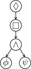
(a) Parse tree $\mathcal{T}$.

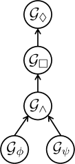
(b) Computation graph $\mathcal{G}$.

                                     

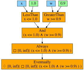
(c) Visualization of $\mathcal{G}$ using the stlcg toolbox.

Figure 2: An illustration of a parse tree (left) and a computation graph (middle) for an STL formula $\lozenge\,\square\,(\phi\wedge\psi)$ where $\phi=w\geq 0.9$ and $\psi=x\leq 1.0$. On the right is a visualization generated from the stlcg toolbox. The blue nodes represent input signals ($x$ and $w$) into the computation graph, the green nodes represent parameters of the predicates, and the orange nodes represent STL operations.

An example of a parse tree $\mathcal{T}_{\theta}$ for a formula $\theta=\lozenge\,\square\,(\phi\wedge\psi)$ is illustrated in Figure 2a where $\phi$ and $\psi$ are assumed to be predicates. By flipping the direction of all the edges in $\mathcal{T}_{\theta}$, we obtain a directed acyclic graph $\mathcal{G}_{\theta}$, shown in Figure 2b. At a high level, signals are passed through the root nodes, $\mathcal{G}_{\phi}$ and $\mathcal{G}_{\psi}$, to produce $\tau(s,\phi)$ and $\tau(s,\psi)$, robustness traces of $\phi$ and $\psi$. The robustness traces are then passed through the next node of the graph, $\mathcal{G}_{\wedge}$, to produce the robustness trace $\tau(s,\phi\wedge\psi)$, and so forth until the root node is reached and the output is $\tau(s,\lozenge\,\square\,(\phi\wedge\psi))$.

3 STL Robustness Formulas as Computation Graphs

We first describe how to represent each STL robustness formula described in (2) as a computation graph, and then show how to combine them together to form the overall computation graph that computes the robustness trace of any given STL formula. Further, we provide smooth approximations to the $\max$ and $\min$ operations to help make the gradients smoother when backpropagating through the graph, and introduce a new robustness formula which addresses some limitations of using the $\max$ and $\min$ functions. The resulting computational framework, stlcg, is implemented using PyTorch (Paszke et al., 2017) and the code can be found at https://github.com/StanfordASL/stlcg. Further, this toolbox includes a graph visualizer, illustrated in Figure 2c, to show the graphical representation of the STL formula and how it depends on the inputs and parameters from the predicates.

3.1 Computation Graphs and Backpropagation

A computation graph is a directed graph where the nodes correspond to operations or variables. Variable values are passed through operation nodes, and the outputs can feed into other nodes and so forth. For example, the computation graph of the mathematical operation $z=w(x+y)$ is illustrated in Figure 3 where $x$, $y$, and $w$ are inputs into the graph, $+$ and $\times$ are mathematical operations, and $z$ is the output.

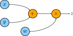
Figure 3: Computation graph of the mathematical operation $z=w(x+y)$.

When the operations are differentiable, we can leverage the chain rule and therefore backpropagate through the computation graph to obtain derivatives of the output with respect to any variable that the output depends on.

3.2 Computation Graphs of STL Operators

First, we consider the computation graph of each STL robustness formula given in Section 2.2 individually.

3.2.1 Non-temporal STL Operators

The robustness formulas for the non-temporal operators are relatively straightforward to implement as computation graphs because they involve simple mathematical operations, such as subtraction, $\max$, and $\min$, and do not involve looping over time. The computation graph for a predicate ($\mu_{c}$), negation ($\neg$), implies ($\Rightarrow$), and ($\wedge$), and or ($\vee$) are illustrated in Figure 5. The input $x$ (and $y$) is either the signal of interest (for predicates) or the robustness trace(s) of a subformula(s) (for non-predicate operators). While the output $z$ is the robustness trace after applying the corresponding STL robustness formula. For example, when computing the robustness trace of $\phi\wedge\psi$ for a signal $s$, the inputs for $\mathcal{G}_{\wedge}$ are $\tau(s,\phi)$ and $\tau(s,\psi)$, and the output is $\tau(s,\phi\wedge\psi)$.

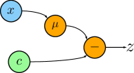
(a) $\mathcal{G}_{\mu_{c}}$

            

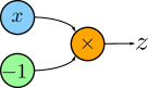
(b) $\mathcal{G}_{\neg}$

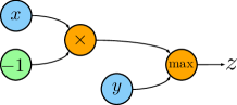
(c) $\mathcal{G}_{\Rightarrow}$

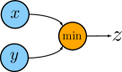
(d) $\mathcal{G}_{\wedge}$

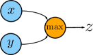
(e) $\mathcal{G}_{\vee}$

Figure 5: An illustration the computation graph representing the STL robustness formula for (a) predicates, (b) negation, (c) implies, (d) and, and (e) or. Blue nodes denote input variables, green nodes denote parameter values, and orange nodes denote mathematical operations.

3.2.2 Temporal STL Operators

Due to the temporal nature of the eventually $\lozenge_{[a,b]}$, always $\square_{[a,b]}$, and until $\mathcal{U}_{[a,b]}$ operators, the computation graph construction needs to be treated differently than the non-temporal operators. While computing the robustness value of any temporal operators given an input signal is straightforward, computing the robustness trace in a computationally efficient way is less so. To accomplish this, we apply dynamic programming (Fainekos et al., 2012) by using a recurrent computation graph structure, similar to the recurrent structure of recurrent neural networks (RNN) (Hochreiter and Schmidhuber, 1997). In doing so, we can compute the robustness value for every subsignal of an input signal. The complexity of this approach is linear in the length of the signal for $\lozenge$ and $\square$, and at most quadratic for the $\mathcal{U}$ operator.

3.2.3 Eventually and Always Operators

We first consider the Eventually operator, noting that similar a construction applies for the Always operator. Let $\psi=\lozenge_{[a,b]}\phi$ ; the goal is to construct the computation graph $\mathcal{G}_{\lozenge_{[a,b]}}$ which takes as input $\tau(s,\phi)$ (the robustness trace of the subformula) and outputs $\tau(s,\lozenge_{[a,b]}\phi)$. For ease of notation, we denote $\rho(s_{t_{i}},\phi)=\rho_{i}^{\phi}$ as the robustness value of $\phi$ for subsignal $s_{t_{i}}$. Figure 6 illustrates the unrolled graphical structure of $\mathcal{G}_{\lozenge_{[a,b]}}$. the $i$-th recurrent (orange) node takes in a hidden state $h_{i}$ and an input state $\rho_{T-i}^{\phi}$, and produces an output state $o_{T-i}$ (note the time indices are reversed in order to perform dynamic programming). By collecting all the $o_{i}$’s, the outputs of the computation graph form the (backward) robustness trace of $\psi$, i.e., $\tau(s,\psi)$. The output robustness trace is treated as the input to another computation graph representing the next STL operator dictated by $\mathcal{G}$.

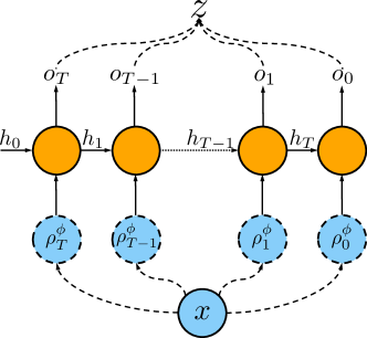
Figure 6: A schematic of an unrolled recurrent computation graph for the $\lozenge$ (eventually) and $\square$ (always) temporal operators, differing in the implementation of the recurrent cells depicted as orange circles. The dashed lines indicate the decomposition/reconstruction of the input/output signal via the time dimension.

	$h_{0}$	$o_{5}$	$h_{1}$	$o_{4}$	$h_{2}$	$o_{3}$	$h_{3}$	$o_{2}$	$h_{4}$	$o_{1}$	$h_{5}$	$o_{0}$
$\lozenge_{[0,t_{T}]}(s>0)$	1	1	1	3	3	3	3	3	3	3	3	3
$\lozenge_{[0,2]}(s>0)$	(1, 1)	1	(1, 1)	3	(1, 3)	3	(3, 2)	3	(2, 1)	2	(1, 1)	1
$\lozenge_{[2,t_{T}]}(s>0)$	(1,(1,1))	1	(1,(1,1))	1	(1,(1,3))	1	(1,(3,2))	3	(3,(2,1))	3	(3,(1,1))	3
$\lozenge_{[1,3]}(s>0)$	(1, 1, 1)	1	(1, 1, 1)	1	(1, 1, 3)	3	(1, 3, 2)	3	(3, 2, 1)	3	(2, 1, 1)	2

Table 1: Hidden and output states of $\lozenge_{\mathrm{I}}(s>0)$ for a signal $s=1,1,1,2,3,1$ and different time intervals $\mathrm{I}$. The signal is fed into the computation graph backward.

Before describing the mechanics of the computation graph $\mathcal{G}_{\lozenge_{[a,b]}}$, we first define $M_{N}\in\mathbb{R}^{N\times N}$ to be a square matrix with ones in the upper off-diagonal and $B_{N}\in\mathbb{R}^{N}$ to be a vector of zeros with a one in the last entry. If $x\in\mathbb{R}^{N}$ and $u\in\mathbb{R}$, then the operation $M_{N}x+B_{N}u$ removes the first element of $x$, shifts all the entries up one index and replaces the last entry with $u$. We distinguish four variants of $\mathcal{G}_{\lozenge_{[a,b]}}$ which depends on the interval $[a,b]$ attached to the temporal operator.

. Let the initial hidden state be $h_{0}=\rho_{T}^{\phi}$. The hidden state is designed to keep track of the largest value the graph has processed so far. The output state for the first step is $o_{T}=\max(h_{0},\rho_{T}^{\phi})$, and the next hidden state is defined to be $h_{1}=o_{T}$. Hence the general update step becomes,

$$h_{i+1}=o_{T-i},\quad o_{T-i}=\max(h_{i},\rho_{T-i}^{\phi}).$$

By construction, the last step in this dynamic programming procedure,

$$o_{0} =\max(h_{T},\rho_{0}^{\phi})$$

$$o_{0} =\max(\max(h_{T-1},\rho_{1}^{\phi}),\rho_{0}^{\phi})$$

$$\vdots$$

$$o_{0} =\max(h_{0},\rho_{T}^{\phi},\rho_{T-1}^{\phi},\ldots,\rho_{0}^{\phi})$$

$$o_{0} =\rho(s_{t_{0}},\lozenge\,\phi).$$

The output states of $\mathcal{G}_{\lozenge\phi}$, $o_{0},\,o_{1},\ldots,\,o_{T}$, form $\tau(s,\lozenge\phi)$, the robustness trace of $\psi=\lozenge\phi$, and the last output state $o_{0}$ is $\rho(s,\lozenge\,\phi)$.

. Let the initial hidden state be $h_{0}=(h_{0_{1}},\,h_{0_{2}},\,\ldots,\,h_{0_{N-1}})$, where $h_{0_{i}}=\rho_{T}^{\phi},\>\forall i=1,...,N-1$ and $N$ is the number of time steps contained in the interval $[0,b]$. The hidden state is designed to keep track of inputs in the interval $(t_{i},t_{i}+b]$. The output state for the first step is $o_{T}=\max(h_{0},\rho_{T}^{\phi})$ (the $\max$ operation is over the elements in $h_{0}$ and $\rho_{T}^{\phi}$), and the next hidden state is defined to be $h_{1}=M_{N-1}h_{0}+B_{N-1}\rho_{T}^{\phi}$. Hence the general update step becomes,

$$h_{i+1} =M_{N-1}h_{i}+B_{N-1}\rho_{T-i}^{\phi},$$

$$o_{T-i} =\max(h_{i},\rho_{T-i}^{\phi}).$$

By construction, $o_{0}$ corresponds to the definition of $\rho(s_{t_{0}},\lozenge_{[0,b]}\phi)$, $b<t_{T}$.

. Let the hidden state be a tuple $h_{i}=(c_{i},\,d_{i})$. Intuitively, $c_{i}$ keeps track of the maximum value over future time steps starting from time step $t_{i}$, and $d_{i}$ keeps track of all the values in the time interval $[t_{i},t_{i}+a]$. Specifically, $d_{i_{1}}=\rho_{t_{i}+a}^{\phi}$. Let the initial hidden state be $h_{0}=(\rho_{T}^{\phi},d_{0})$ where $d_{0}=(d_{0_{1}},\,d_{0_{2}},\,\ldots,\,d_{0_{N-1}})$, $d_{0_{i}}=\rho_{T}^{\phi},\>\forall i=1,...,N-1$ and $N$ is the number of time steps encompassed in the interval $[0,a]$. The output for the first step is $o_{T}=\max(c_{0},\,d_{0_{1}})$, and the next hidden state is defined to be $h_{1}=(o_{T},\,M_{N-1}d_{0}+B_{N-1}\rho_{T}^{\phi}$). Following this pattern, the general update step becomes,

$$h_{i+1} =(o_{T-i},\,M_{N-1}d_{i}+B_{N-1}\rho_{T-i}^{\phi}),$$

$$o_{T-i} =\max(c_{i},\,d_{i_{1}}).$$

By construction, $o_{0}$ corresponds to the definition of $\rho(s_{t_{0}},\lozenge_{[a,t_{T}]}\phi)$, $a>0$.

. Let the initial hidden state be $h_{0}=(h_{0_{1}},\,h_{0_{2}},\,\ldots,\,h_{0_{N-1}})$, where $h_{0_{i}}=\rho_{T}^{\phi},\>\forall i=1,...,N-1$ and $N$ is the number of time steps encompassed in the interval $[0,b]$. The hidden state is designed to keep track of all the values between $(t_{i},t_{i}+b]$. Let $M$ be the number of time steps encompassed in the $[a,b]$ interval. The output for the first step is $o_{T}=\max(h_{0_{1}},\,h_{0_{2}},\,\ldots,\,h_{0_{M}})$. The next hidden state is defined to be $h_{1}=M_{N-1}h_{0}+B_{N-1}\rho_{T}^{\phi}$. Hence the general update step becomes,

$$h_{i+1} =M_{N-1}h_{i}+B_{N-1}\rho_{T-i}^{\phi},$$

$$o_{T-i} =\max(h_{i_{1}},\,h_{i_{2}},\,\ldots,\,h_{i_{M}})$$

By construction, $o_{0}$ corresponds to the definition of $\rho(s_{t_{0}},\lozenge_{[a,b]}\phi)$, $a>0$, $b<t_{T}$.

The computation graph for the Always operation is the same but instead uses the $\min$ operation instead of $\max$. The time complexity for computing $\tau(s,\lozenge_{[a,b]}\phi)$ (and also $\tau(s,\square_{[a,b]}\phi)$) is $\mathcal{O}(T)$ since it requires only one pass through the signal. See Example 4 for a concrete example.

Example 4.

Let the values of a signal be $s=1,1,1,2,3,1$. Then the hidden and output states for $\lozenge_{I}$ with different intervals $I$ are given in Table 1.

3.2.4 Until Operator

Recall that the robustness formula for the Until operator is,

$$\rho(s_{t},\phi\,\mathcal{U}_{[a,b]}\psi)=\max_{t^{\prime}\in[t+a,t+b]}\min\{\rho(s_{t^{\prime}},\psi),\min_{\tau\in[t,t^{\prime}]}\rho(s_{\tau},\phi)\}.$$

Using the definition of the Always robustness formula, the Until robustness formula can be rewritten as,

$$\rho(s_{t},\phi\,\mathcal{U}_{[a,b]}\psi)=\max_{t^{\prime}\in[t+a,t+b]}\min\{\rho(s_{t^{\prime}},\psi),\rho(s_{t}^{t^{\prime}},\square\phi)\}$$ (3)

where $s_{t}^{t^{\prime}}$ denotes a signal consisting of values from $t$ to $t^{\prime}$. Before we describe the computation needed for different instantiations of $[a,b]$, we first define the following notation. Let $\overleftarrow{s}_{t}^{t_{i}}$ denote the reversed signal of $s_{t}^{t_{i}}$. We also want to note that the inputs into $\mathcal{G}_{\phi\mathcal{U}_{[a,b]}\psi}$ are $\tau(s_{t},\phi)$ and $\tau(s_{t},\psi)$.

. Suppose we have a signal $s_{t_{0}}$. For each time step $t_{i}$, we can easily compute $\tau(s_{t_{0}}^{t_{i}},\square\phi)$ (using the methodology outlined in Section 3.2.3). Therefore, we can compute $\min\{\rho(s_{t_{i}},\psi),\rho(s_{t_{j}}^{t_{i}},\square\phi)\}$ for all subsignals of $s_{t_{0}}^{t_{i}}$. After looping through all $t_{i}$’s, we can perform the outer maximization in (3) and therefore produce $\tau(s_{t_{0}},\phi\,\mathcal{U}\,\psi)$. Since we looped through all the values of $s_{t_{0}}$ once and computed the robustness trace of $\square\,\phi$ within each iteration, the time complexity is $\mathcal{O}(T^{2})$ where $T$ is the length of the signal.

First, loop through each time $t_{i}$. Each iteration of this loop will produce $\rho(s_{t_{i}},\phi\,\mathcal{U}_{[a,b]}\psi)$, the robustness value for subsignal $s_{t_{i}}$. For a given $t_{i}$, we can compute $\rho(s_{t_{i}}^{t^{\prime}},\square\phi)$ for all $t^{\prime}\in[t_{i}+a,t_{i}+b]$ by computing the robustness trace of $\square\phi$ over $\overleftarrow{s}_{t_{i}}^{t_{i}+b}$ and then taking the the last $N$ values of robustness trace where $N$ is the number of time steps inside $[a,b]$. As such, we can compute $\rho(s_{t_{i}},\phi\,\mathcal{U}_{[a,b]}\,\psi)=\max_{t^{\prime}\in[t_{i}+a,t_{i}+b]}\min\{\rho(s_{t^{\prime}},\psi),\rho(s_{t_{i}}^{t^{\prime}},\square\phi)\}$. Since we loop through all time steps in the signal, and compute the Always robustness trace over $\overleftarrow{s}_{t_{i}}^{t_{i}+b}$, the time complexity is $\mathcal{O}(TM)$ where $T$ is the length of the signal, and $M$ is the number of time steps contained in $[0,b]$.

This is the same as Case 2 but instead we compute $\rho(s_{t_{i}}^{t^{\prime}},\square\phi)$ for all $t^{\prime}\in[t_{i}+a,t_{T}]$ (practically speaking, we just consider up until the end of the signal). The time complexity in this case is $\mathcal{O}(T^{2})$.

We have just described how we can compute the robustness trace of the Until operation by leveraging the computation graph construction of the Always operator and a combination of for loops, and $\max$ and $\min$ operations, all of which can be expressed using computation graphs.

3.3 Calculating Robustness with Computation Graphs

Since we can now construct the computation graph corresponding to each STL operator of a given STL formula, we can now construct the computation graph $\mathcal{G}$ by stacking together computation graphs according to $\mathcal{T}$, the corresponding parse tree. The overall computation graph $\mathcal{G}$ takes a signal $s$ as its input, and outputs the robustness trace as its output. The total time complexity of computing the robustness trace for a given STL formula is at most $\mathcal{O}(|\mathcal{T}|T^{2})$ where $|\mathcal{T}|$ is the number of nodes in $\mathcal{T}$, and $T$ is the length of the input signal.

By construction, the robustness trace generated by the computation graph matches exactly the true robustness trace of the formula, and thus stlcg is correct by construction (see Theorem 1).

Theorem 1 (Correctness of stlcg).

For any STL formula $\phi$ and any signal $s$, let $\mathcal{G}_{\phi}$ be the computation graph produced by stlcg. Then passing a signal $s$ through $\mathcal{G}_{\phi}$ produces the robustness trace $\tau(s,\phi)$.

3.4 Smooth Approximations to stlcg

Due to the recursion over $\max$ and $\min$ operations, there is the potential for many of the gradients be zero and therefore potentially leading to numerical difficulties. To mitigate this, we can leverage smooth approximations to the $\max$ and $\min$ functions. Let $x\in\mathbb{R}^{n}$ and $\beta\in\mathbb{R}_{\geq 0}$. We can use either the softmax/min or logsumexp approximations,

$$\widetilde{\max}_{\beta}(x) =\frac{\sum_{i}^{n}x_{i}\exp(\beta x_{i})}{\sum_{j}^{n}\exp(\beta x_{j})}\>\text{or}\>\frac{1}{\beta}\log\sum_{i=1}^{n}\exp(\beta x_{i})$$

$$\widetilde{\min}_{\beta}(x) =\frac{\sum_{i}^{n}x_{i}\exp(-\beta x_{i})}{\sum_{j}^{n}\exp(-\beta x_{j})}\>\text{or}\>-\frac{1}{\beta}\log\sum_{i=1}^{n}\exp(-\beta x_{i})$$

where $x_{i}$ represents the $i$-th element of $x$, and $\beta$ operates as a scaling parameter. The approximation approaches the true solution when $\beta\rightarrow\infty$ while $\beta\approx 0$ results in the mean value of the entries of $x$. In practice, $\beta$ can be annealed over gradient-descent iterations.

Further, $\max$ and $\min$ are pointwise functions. As a result, the robustness of an STL formula can be highly sensitive to one single point in the signal, potentially providing an inadequate robustness metric especially if the signal is noisy (Mehdipour et al., 2019), or causing the gradients to accumulate to a single point only. We propose using an integral-based STL robustness formula $\mathcal{I}^{M}_{[a,b]}$ to “spread out” the gradients, and it is defined as follows. For a given weighting function $M(t)$,

$$\rho(s_{t},\mathcal{I}^{M}_{[a,b]}\phi)=\sum_{\tau=t+a}^{t+b}M(\tau)\rho(s_{\tau},\phi).$$

The integral robustness formula considers the weighted sum of the input signal over an interval $[a,b]$ and therefore produces a smoother robustness trace and the implication of this is demonstrated in Section 4.1.

4 Case Studies: Using stlcg for Robotics Applications

We demonstrate the versatility and computational advantages of using stlcg by investigating a number of case studies in this section. In these examples, we show (i) how our approach can be used to incorporate logical requirements into motion planning problems (Section 4.1), (ii) the computational efficiency of stlcg achieved via parallelization and batching (Section 4.2), and (iii) how we can use stlcg to translate human-domain knowledge into a form that can be integrated with deep neural networks (Section 4.3). Code can be found at https://github.com/StanfordASL/stlcg.

4.1 Motion Planning with STL Constraints

Recently, there has been a lot of interest in motion planning with STL constraints (e.g., Pant et al. (2017); Raman et al. (2014)); the problem of finding a sequence of states and controls that drives a robot from an initial state to a final state while obeying a set of constraints which includes STL specifications. For example, while reaching a goal state, a robot may be required to enter a particular region for three time steps before moving to its final destination. Rather than reformulating the problem as a MILP to account for STL constraints as done in Raman et al. (2014), we consider a simpler approach of augmenting the loss function with an STL robustness term, and therefore enable a higher degree of customization when designing how the STL specifications are factored into the problem.

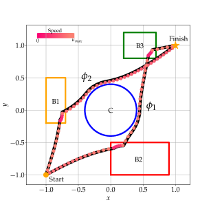
(a) Trajectories satisfying $\phi_{1}$ and $\phi_{2}$ which uses the Always operator.

(b) Trajectories satisfying $\psi_{1}$ and $\psi_{2}$ which uses the integral operator.

            

Figure 7:

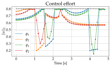
Figure 8:

4.1.1 Motion Planning Example 1

Consider the following motion planning problem illustrated in Figure 7; a robot must find a sequence of states $X=x_{1:N}$ and controls $U=u_{1:N-1}$ that takes it from the yellow circle (position = $(-1,-1)$) to the yellow star (position=$(1,1)$) while satisfying an STL constraint $\phi$. Assume the robot is a point mass with state $x\in\mathbb{R}^{2}$ and action $u\in\mathbb{R}^{2}$. It obeys single 2D integrator dynamics $\dot{x}=u$ and has a control constraint $\|u\|_{2}\leq u_{\max}$. We can express the control constraint as an STL formula: $\theta=\square\,\|u\|_{2}\leq u_{\max}$.

This motion planning problem can be cast as an unconstrained optimization problem ,

$$\min_{X,\,U}\>\|Ez-D\|_{2}^{2}+\gamma_{1}J_{m}(\rho(X,\phi))+\gamma_{2}J_{m}(\rho(U,\theta))$$

where $z=(X,U)$ is the concatenated vector of states and controls . Since the dynamics are linear, we can express the dynamics, and start and end point constraints across all time steps in a single linear equation $Ez=D$. The other function, $J_{m}$, represents the cost on the STL robustness value with margin $m$. We use $J_{m}(x)=\mathrm{ReLU}(-(x-m))$ where $\mathrm{ReLU}(x)=\max(0,x)$ is the rectified linear unit. This choice of $J_{m}$ incentivizes the robustness value to be greater or equal to the margin $m$.

To showcase a variety of STL constraints, we consider four different STL specifications,

$$\phi_{1} =\lozenge\square_{[0,5]}\text{inside B2}\wedge\lozenge\square_{[0,5]}\text{inside B3}\wedge\square\neg\text{inside C}$$

$$\phi_{2} =\lozenge\square_{[0,5]}\text{inside B1}\wedge\square\neg\text{inside B3}\wedge\square\neg\text{inside C}.$$

$$\psi_{1} =\lozenge\mathcal{I}^{\Delta t^{-1}}_{[0,5]}\text{inside B2}\wedge\lozenge\mathcal{I}^{\Delta t^{-1}}_{[0,5]}\text{inside B3}\wedge\square\neg\text{inside C}$$

$$\psi_{2} =\lozenge\mathcal{I}^{\Delta t^{-1}}_{[0,5]}\text{inside B1}\wedge\neg\mathcal{I}^{\Delta t^{-1}}\text{inside B3}\wedge\square\neg\text{inside C},$$

where B1, B2, B3, and C are the regions illustrated in Figure 7. $\phi_{1}$ translates to: the robot needs to eventually stay inside the red box (B2) and green box (B3) for five time steps each, and never enter the blue circular region (C). Similarly, $\phi_{2}$ translates to: the robot eventually needs to stay inside the orange box (B1) for five time steps, and never enter the green box (B3) nor the blue circular region (C). $\psi_{1}$ and $\psi_{2}$ are similar to $\phi_{1}$ and $\phi_{2}$ except that the integral robustness formula (described in Section 3.4) is used.

We initialize the solution with a straight line connecting the start and end points, noting that this initialization violates the STL specification. We then perform standard gradient descent (constant step size of 0.05) with $\gamma_{1}=\gamma_{2}=0.3$, $m=0.05$, and $\Delta t^{-1}=\frac{1}{0.1}$; the solutions are illustrated in Figure 7. As anticipated, using the integral robustness formula results in a smoother trajectory and smoother control signal than using the Always robustness formula. We also note that the control constraint ($u_{\max}=0.8$) was satisfied for all cases (see Figure 8).

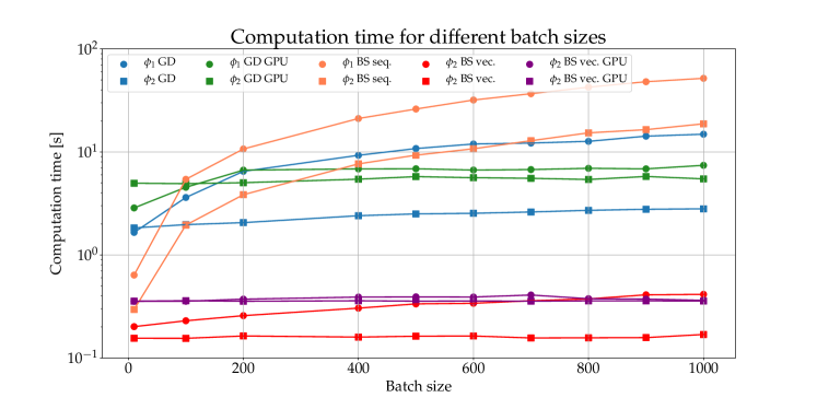
Figure 11: The experiments were computed using a 3.0GHz octocore AMD Ryzen 1700 CPU and a Titan X (Pascal) GPU.

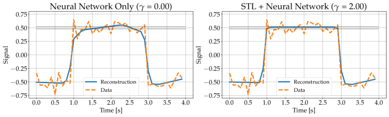
Figure 12: A simple supervised learning problem without (left) and with (right) STL regularization. The output is required to satisfy $\phi=\square_{[1,2.75]}(s>0.48\,\wedge\,s<0.52)$ despite the training data being noisy and violating $\phi$.

4.2 Parametric STL for Behavioral Clustering

In this example, we consider parametric STL (pSTL) problems (Vazquez-Chanlatte et al., 2017; Asarin et al., 2012), and demonstrate that since modern automatic differentiation software such as PyTorch can be used to implement stlcg, we have the ability to very easily parallelize the computation and leverage GPU hardware. The pSTL problem is a form of logic-based parameter estimation for time series data. It involves first constructing an STL template formula where the predicate parameter values and/or time intervals are unknown. The goal is to find parameter values that best fit a given signal. As such, the pSTL process can be viewed as a form of feature extraction for time-series data. Logic-based clustering can be performed by clustering on the extracted pSTL parameter values. For example, pSTL has been used to cluster human driving behaviors in the context of autonomous driving applications (Vazquez-Chanlatte et al., 2017).

The experimental setup for our example is as follows. Given a dataset of $N$ step responses from randomized second-order systems, we use pSTL to help cluster different types of responses, e.g., under-damped, critically damped, or over-damped. Based on domain knowledge of second order step responses, we design the following pSTL formulas,

$$\qquad\phi_{1} =\square_{[50,100]}\,|s-1|<\epsilon_{1}$$ (final value)

$$\qquad\phi_{2} =\square\,s<\epsilon_{2}$$ (peak value)

For each signal $s^{(j)},\,j=1,\,\ldots,\,N$, we want to find $\epsilon_{1j}$ and $\epsilon_{2j}$ ($\epsilon_{1}$ and $\epsilon_{2}$ for the $j$th signal) that provides the best fit, i.e., robustness equals zero. Using stlcg, we can batch our computation and hence solve for all $\epsilon_{ij}$ more efficiently.

Both approaches converged to the same solution, and the resulting computation times are illustrated in Figure 11.

For cases where the solution has multiple local minima (e.g., non-monotonic pSTL formulas), additionally batch the input with samples from the parameter space, and anneal $\beta$, the scaling parameter for the $\max$ and $\min$ approximation over each iteration. The samples will converge to a local minimum, and, with sufficiently many samples and an adequate annealing schedule, we can (hopefully) find the global minimum. However, we note that we are currently not able to optimize time parameters that define an interval as we cannot backpropagate through those parameters. Future work will investigate how to address this, potentially leveraging ideas from forget gates in long short-term memory (LSTM) networks Gers et al. (1999).

4.3 Robustness-Aware Neural Networks

We demonstrate via a number of small yet illustrative examples how stlcg can be used to make learning-based models (e.g., deep neural networks) more robust and reflective of desired behaviors stemming from human-domain knowledge.

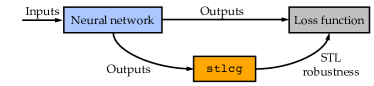
Figure 13: Architecture of a neural network enhanced with STL regularization in its loss function.

4.3.1 Model Fitting with Known Structure

In this example, we show how stlcg can be used to regularize a neural network model to prevent overfitting to the noise in the data. Consider the problem of using a neural network to model temporal data such as the (noisy) signal shown by the orange line in Figure 12. Suppose that based on domain knowledge of the problem, we know that the data must satisfy the STL formula $\phi=\square_{[1,2.75]}(s>0.48\,\wedge\,s<0.52)$. Due to the noise in the data, $\phi$ is violated. Neural networks are prone to overfitting and may unintentionally learn this noise. We can train a single layer neural network $f_{\theta}$ to capture the bump-like behavior in the noisy data. However, this learned model violates $\phi$ (see Figure 12 (left)). To mitigate this, we regularize the learning processing by augmenting the loss function with a term that penalizes negative robustness values. Specifically, the loss function becomes

$$\mathcal{L}=\mathcal{L}_{0}+\gamma\mathcal{L}_{\mathrm{STL}}$$ (5)

where $\mathcal{L}_{0}$ is the original loss function (e.g., reconstruction loss), and, in this example, $\mathcal{L}_{\mathrm{STL}}=\mathrm{ReLU}(-\rho(f_{\theta}(x),\phi))$ is the robustness loss evaluated over the neural network output, and $\gamma=2$. A schematic representing how, in general, a neural network can be regularized using stlcg is illustrated in Figure 13.

As shown in Figure 12 (right), the model with robustness regularization is able to obey $\phi$ more robustly. Note that regularizing the loss function with an STL loss does not guarantee that the output will satisfy $\phi$ but rather the resulting model is encouraged to violate $\phi$ as little as possible, and the incentive can be controlled by the parameter $\gamma$.

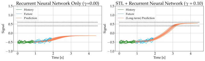
Figure 14: Comparison of a sequence-to-sequence prediction model without (left) and with (right) robustness regularization. With robustness regularization, the model achieves desired long-term behavior $\phi=\lozenge\,\square_{[0,1]}\,(s>0.4\,\wedge\,s<0.6)$ despite having access to only short-term behaviors during training.

4.3.2 Sequence-to-Sequence Prediction

In this example, we demonstrate how stlcg can be used to influence long-term behaviors of sequence-to-sequence prediction problems to reflect domain knowledge despite only having access to short-term data. Sequence-to-sequence prediction models are often used in robot decision-making, such as in the context of model-based control where a robot may predict future trajectories of other agents in the environment given past trajectories, and use these predictions for decision-making and control (Schmerling et al., 2018). Often contextual knowledge of the environment is not explicitly labeled in the data, for instance, cars always drive on the right side of the road, or drivers tend to keep a minimum distance from other cars. stlcg provides a natural way, in terms of language and computation, to incorporate contextual knowledge into the neural network training process, thereby infusing desirable behaviors into the model which, as demonstrated through this example, can improve long-term prediction performance.

Figure 15: Schematic of a rolled-out RNN network illustrating how to leverage stlcg to improve long-term predictions with access to only short-term data.

We generate a dataset of signals $s$ by adding noise to the $\tanh$ function with random scaling and offset. Illustrated in Figure 15, we design an LSTM encoder that takes the first 10 time steps as inputs (i.e., trajectory history). The encoder is connected with an LSTM decoder network that predicts the next 10 time steps (i.e., future trajectory). Note, the time steps are of size $\Delta t=0.1$. Suppose, based on contextual knowledge, we know a priori that the signal will eventually, beyond the next ten time steps captured in the data, be in the interval $[0.4,0.6]$. Specifically, the signal will satisfy $\phi=\lozenge\,\square_{[0,1]}\,(s>0.4\,\wedge\,s<0.6)$. We can leverage knowledge of $\phi$ by rolling out the RNN model over an extended time horizon beyond what is provided in the training data, and apply the robustness loss on the rolled-out signal $s^{(i)}$ corresponding to the input $x^{(i)}$. We use (5) as the loss function where $\mathcal{L}_{0}$ is the mean square error reconstruction loss over the first ten predicted time steps, and $\mathcal{L}_{\mathrm{STL}}=\sum_{i}\mathrm{ReLU}(-\rho(s^{(i)},\phi))$ is the total amount of violations over the extended roll-out. With $\gamma=0.1$, Figure 14 illustrates that with STL robustness regularization, the RNN model can successfully predict the next ten time steps and also achieve the desired long-term behavior despite being only trained on short-horizon data.

4.3.3 Latent Space Structure

In this example, we demonstrate how stlcg can be used to enforce logic-based interpretable structure into deep latent space models and thereby improve model performance. Deep latent space models are a type of neural network models that introduce a bottleneck in the architecture to force the model to learn salient (i.e., latent) features from the input in order to (potentially) improve modeling performance and provide a degree of interpretability. Specifically, an encoder network transforms the inputs into latent variables, which have a lower dimension than the inputs, and then a decoder network transforms the latent variables into desired outputs. An illustration of an encoder-decoder architecture is shown in Figure 16 in blue.

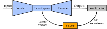
Figure 16: Architecture of a latent space model leveraging stlcg for added structure.

Variational autoencoders (VAEs) (Kingma and Welling, 2013) are a type of probabilistic deep latent space models used in many domains such as image generation, and trajectory prediction. Given a dataset, a VAE strives to learn a distribution such that samples drawn from the distribution will be similar to what is represented in the dataset (e.g., given a dataset of human faces, a VAE can generate new similarly-looking images of human faces). For brevity, we omit describing details of VAEs but refer the reader to Doersch (2016); Jang et al. (2017) for an overview on VAEs.

Unfortunately, the VAE latent representation is learned in an unsupervised manner whereby any notions of interpretability are not explicitly enforced, nor is there any promise that the resulting latent space will adequately encompass human-interpretable features. Developing techniques to add human-understandable interpretability to the latent space representation is currently an active research area (Adel et al., 2018).

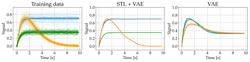
Figure 17: A VAE example leveraging stlcg to provide more structure into the latent space representation. Left: Training data used to train a VAE with a discrete latent space. Middle: Generated outputs from a VAE model leveraging stlcg. Right: Generated outputs from a standard VAE without leveraging stlcg.

In this example, we demonstrate that we can use stlcg to project expert knowledge about the dataset into the latent space construction, and therefore aid in the interpretability of the latent space representation. Consider the following dataset illustrated in Figure 17 (left). The dataset is made up of (noisy) trajectories; Gaussian noise was added onto the trajectories shown in solid color. Notably, the data is multimodal as there are three trajectory archetypes contained in the data, each denoted by different colors. The goal is to learn a VAE model that can generate similar-looking trajectories. However, training a VAE for multimodal data is generally challenging (e.g., can suffer from mode collapse).

We consider a VAE model with a discrete latent space with dimension $N_{z}=3$ because, based on our “expert knowledge”, there are three different types of trajectory modes. The latent variable $z\in\{0,1\}^{3}$ is a one-hot vector of size three, i.e., $z\in\{[1,0,0]^{\top},[0,1,0]^{\top},[0,0,1]^{\top}\}$. Additionally, we use LSTM networks for the encoder and decoder networks due to the sequential nature of the data. Based on our “expert knowledge”, the data satisfies the following STL formula,

$$\phi_{c}=\square_{[7.5,9.75]}\left[(x>c-\epsilon)\wedge(s<c+\epsilon)\right],$$

where $c\in\{0.7,0.35,0\}$ and $\epsilon=0.025$. This STL formula describes the convergence of a signal to a value $c$ within some tolerance $\epsilon$. Let $C=[0.7,0.35,0]^{\top}$ be a column vector corresponding to the possible parameter values of $\phi_{c}$ (based on expert knowledge). Then the dot product $z^{\top}C$ selects the entry of $C$ corresponding to 1’s position in $z$. As such, if $s$ is the output trajectory from the VAE mode, and $z$ is the corresponding latent vector, then we can construct an STL loss, $\mathcal{L}_{\mathrm{STL}}=\mathrm{ReLU}(-\rho(s,\phi_{z^{\top}C}))$. This STL loss enforces each latent vector instantiation to correspond to different STL parameter values and therefore incentives the resulting output to satisfy the associated STL formula. The overall loss function used to train a VAE model with STL information is,

$$\mathcal{L}=\mathcal{L}_{\mathrm{VAE}}+\gamma\mathcal{L}_{\mathrm{STL}},$$

where $\mathcal{L}_{\mathrm{VAE}}$ is the standard loss function used when training a typical VAE model.

Figure 17 (middle) illustrates the trajectories generated from a VAE trained with an additional STL loss $(\gamma=4)$, while Figure 17 (right) showcases trajectories generated with the same model (i.e., same neural network architecture and size) trained without the STL loss $(\gamma=0)$. Note, the hyperparameters using during training (e.g., seed, learning rate, number of iterations, batch size, etc,) were the same across the two models. We can see that by leveraging expert knowledge about the data and encoding that knowledge via STL formulas, we are able to generate outputs that correctly cover the three distinct trajectory modes. With more training iterations, it could be possible, though not guaranteed, that the vanilla VAE model would have been able to capture the three distinct trajectory modes. Nonetheless, this example demonstrates that stlcg could potentially be used to accelerate training processes, and enable models to more rapidly converge to a desirable level of performance.

5 Future Work and Conclusions

In this work, we showed that STL is an attractive language to encode spatio-temporal specifications, either as constraints or a form of inductive bias, for a diverse range of problems studied in the field of robotics. In particular, we proposed a technique, stlcg, which transcribes STL robustness formulas as computation graphs, and therefore enabling the incorporation of STL specifications in a range of problems that rely on gradient-based solution methods. We demonstrate through a number of illustrative examples that we are able to infuse logical structure in a diverse range of robotics problems such as motion planning, behavior clustering, and deep neural networks for model fitting, intent prediction, and generative modeling.

We highlight several directions for future work that extend the theory and applications of stlcg as presented in this paper. The first aims to extend the theory to enable optimization over parameters defining time intervals over which STL temporal operators hold, and to also extend the language to express properties that cannot be expressed by the standard STL language. The second involves investigating how stlcg can help verify and improve the robustness of learning-based components in safety-critical settings governed by spatio-temporal rules, such as in autonomous driving and urban air-mobility contexts. The third is to explore more ways to connect supervised structure induced by logic with unsupervised structure learning present in latent spaces models. This connection may help provide interpretability via the lens of temporal logic for neural networks that are typically difficult to analyze.

References

- Adel et al. (2018) Adel T, Ghahramani Z and Weller A (2018) Discovering interpretable representations for both deep generative and discriminative models. In: Int. Conf. on Machine Learning.
- Asarin et al. (2012) Asarin E, Donzé A, Maler O and Nickovic D (2012) Parametric identification of temporal properties. In: Int. Conf, on Runtime Verification.
- Baier and Katoen (2008) Baier C and Katoen JP (2008) Principles of Model Checking. MIT Press.
- Bartocci et al. (2018) Bartocci E, Deshmukh J, Donzé A, Fainekos G, Maler O, Nickovic D and Sankaranarayanan S (2018) Specification-based Monitoring of Cyber-Physical Systems: A Survey on Theory, Tools and Applications. Springer, pp. 135–175.
- Doersch (2016) Doersch C (2016) Tutorial on variational autoencoders. Available at https://arxiv.org/abs/1606.05908.
- Fainekos et al. (2012) Fainekos G, Sankaranarayanan S, Ueda K and Yazarel H (2012) Verification of automotive control applications using S-TaLiRo. In: American Control Conference.
- Fainekos et al. (2008) Fainekos GE, Girard A, Kress-Gazit H and Pappas GJ (2008) Temporal logic motion planning for dynamic robots. Automatica 45(2): 343–352.
- Finucane et al. (2010) Finucane C, Jing G and Kress-Gazit H (2010) LTLMoP: Experimenting with language, temporal logic and robot control. In: IEEE/RSJ Int. Conf. on Intelligent Robots & Systems.
- Gers et al. (1999) Gers FA, Schmidhuber J and Cummins F (1999) Learning to forget: continual prediction with LSTM. In: Int. Conf. on Artificial Neural Networks.
- Hochreiter and Schmidhuber (1997) Hochreiter S and Schmidhuber J (1997) Long short-term memory. Neural Computation .
- Ivanovic et al. (2021) Ivanovic B, Leung K, Schmerling E and Pavone M (2021) Multimodal deep generative models for trajectory prediction: A conditional variational autoencoder approach. IEEE Robotics and Automation Letters 6(2): 295–302. In Press.
- Jang et al. (2017) Jang E, Gu S and Poole B (2017) Categorial reparameterization with gumbel-softmax. In: Int. Conf. on Learning Representations.
- Kingma and Welling (2013) Kingma DP and Welling M (2013) Auto-encoding variational bayes. Available at https://arxiv.org/abs/1312.6114.
- Kress-Gazit et al. (2018) Kress-Gazit H, Lahijanian M and Raman V (2018) Synthesis for robots: Guarantees and feedback for robot behavior. Annual Review of Control, Robotics, and Autonomous Systems 1: 211–236.
- Liu et al. (2021) Liu W, Mehdipour N and Belta C (2021) Recurrent neural network controllers for signal temporal logic specifications subject to safety constraints. IEEE Control Systems Letters 6: 91 – 96.
- Ma et al. (2020) Ma M, Gao J, Feng L and Stankovic J (2020) STLnet: Signal temporal logic enforced multivariate recurrent neural networks. In: Conf. on Neural Information Processing Systems.
- Maler and Nickovic (2004) Maler O and Nickovic D (2004) Monitoring temporal properties of continuous signals. In: Proc. Int. Symp. Formal Techniques in Real-Time and Fault-Tolerant Systems, Formal Modeling and Analysis of Timed Systems.
- Mehdipour et al. (2019) Mehdipour N, Vasile CI and Belta C (2019) Arithmetic-geometric mean robustness for control from signal temporal logic specifications. In: American Control Conference.
- Mehr et al. (2017) Mehr N, Sadigh D, Horowitz R, Sastry S and Seshia SA (2017) Stochastic predictive freeway ramp metering from signal temporal logic specifications. In: American Control Conference.
- Pant et al. (2017) Pant YV, Abbas H and Mangharam R (2017) Smooth Operator: Control using the smooth robustness of temporal logic. In: IEEE Conf. Control Technology and Applications.
- Paszke et al. (2017) Paszke A, Gross S, Chintala S, Chanan G, Yang E, DeVito Z, Lin Z, Desmaison A, Antiga L and Lerer A (2017) Automatic differentiation in PyTorch. In: Conf. on Neural Information Processing Systems - Autodiff Workshop.
- Pnueli (1977) Pnueli A (1977) The temporal logic of programs. In: IEEE Symp. on Foundations of Computer Science.
- Puranic et al. (2020) Puranic AG, Deshmukh JV and Nikolaidis S (2020) Learning from demonstrations using signal temporal logic. In: Conf. on Robot Learning.
- Raman et al. (2014) Raman V, Donze A, Maasoumy M, Murray RM, Sangiovanni-Vincentelli A and Seshia SA (2014) Model predictive control with signal temporal logic specifications. In: Proc. IEEE Conf. on Decision and Control.
- Schmerling et al. (2018) Schmerling E, Leung K, Vollprecht W and Pavone M (2018) Multimodal probabilistic model-based planning for human-robot interaction. In: Proc. IEEE Conf. on Robotics and Automation.
- Vazquez-Chanlatte et al. (2017) Vazquez-Chanlatte M, Deshmukh JV, Jin X and Seshia SA (2017) Logical clustering and learning for time-series data. Proc. Int. Conf. Computer Aided Verification 10426: 305–325.
- Wongpiromsarn et al. (2011) Wongpiromsarn T, Topcu U, Ozay N, Xu H and Murray RM (2011) TuLiP: A software toolbox for receding horizon temporal logic planning. In: Hybrid Systems: Computation and Control.
- Yaghoubi and Fainekos (2019) Yaghoubi S and Fainekos G (2019) Worst-case satisfaction of STL specifications using feedforward neural network controllers: A lagrange multipliers approach. ACM Transactions on Embedded Computing Systems 18(5s).