Rethinking Default Values: a Low Cost and
Efficient Strategy to Define Hyperparameters

Abstract

Machine Learning (ML) algorithms have been increasingly applied to problems from several different areas. Despite their growing popularity, their predictive performance is usually affected by the values assigned to their hyperparameters (HPs). As consequence, researchers and practitioners face the challenge of how to set these values. Many users have limited knowledge about ML algorithms and the effect of their HP values and, therefore, do not take advantage of suitable settings. They usually define the HP values by trial and error, which is very subjective, not guaranteed to find good values and dependent on the user experience. Tuning techniques search for HP values able to maximize the predictive performance of induced models for a given dataset, but have the drawback of a high computational cost. Thus, practitioners use default values suggested by the algorithm developer or by tools implementing the algorithm. Although default values usually result in models with acceptable predictive performance, different implementations of the same algorithm can suggest distinct default values. To maintain a balance between tuning and using default values, we propose a strategy to generate new optimized default values. Our approach is grounded on a small set of optimized values able to obtain predictive performance values better than default settings provided by popular tools. After performing a large experiment and a careful analysis of the results, we concluded that our approach delivers better default values. Besides, it leads to competitive solutions when compared to tuned values, making it easier to use and having a lower cost. We also extracted simple rules to guide practitioners in deciding whether to use our new methodology or a HP tuning approach.

1 Introduction

The last decades have seen an explosion of Machine Learning (ML)studies and applications, promoting and democratizing its usage by people from diverse scientific and technological backgrounds. Progresses in this area have enabled a large uptake of solutions by the industry and research communities. Building an ML solution requires different decisions, and one of them is to choose a suitable algorithm to solve the problem at hand. Different problems present different characteristics, and as a consequence, require different ML algorithms.

Most of these algorithms have hyperparameters (HPs)whose values directly influence their biases, and consequently, the predictive performance of the induced models. Although the number of ML tools available and their popularity has increased, users still struggle to define the best HP settings. This is not a straightforward task and may mislead practitioners to choose one algorithm over another. Usually, users adjust the HP values by trial and error, i.e., they empirically evaluate different settings and select what appear to be the best of them.

Ideally, the HP values should be defined for each problem [8, 43, 38], trying to find the (near) best settings through an optimization process. As a consequence, several tuning techniques have been used for this purpose. The most simple, and often used, are Grid Search (GS)and Random Search (RS) [7]. The former is more suitable for low dimensional problems, i.e., when there are few HPs to set. For more complex scenarios, GS is unable to explore finer promising regions due to the large hyperspace. The latter is able to explore any possible solution of the hyperspace, but also does not perform an informed search, which may lead to a high computational cost.

Meta-heuristics have also been used for HP tuning, having the advantage of performing informed searches. Population-based methods, such as Genetic Algorithms (GAs) [4], Particle Swarm Optimization (PSO) [23] and Estimation of Distribution Algorithms (EDAs) [38], have been largely explored in the literature due to their faster convergence. Sequential Model-based Optimization (SMBO) [49] is a more recent technique that has drawn a large deal of attention, mainly due to its probabilistic nature. It replaces the target function (ML algorithm) by a surrogate model [9], which is faster to compute. However, SMBO itself has many HPs and does not eliminate the shortcoming of having to iteratively evaluate the function to be optimized. All these techniques are valuable alternatives to GS and RS, but they might have a high computational cost, since a large number of candidate solutions usually needs to be evaluated.

A computationally cheaper alternative is to use the default HP setting suggested by most of the ML tools. These settings may be fixed a priori, regardless of the problem, or defined according to some simple characteristics of the data under analysis. For instance, the default values of the number of variables selected for each split of the Random Forest (RF)algorithm [13] and the width of the Gaussian kernel of Support Vector Machines (SVMs) [17] are usually defined based on the number of predictive features.

If on the one hand, default values reduce the subjectivity in the experiments, on the other they may not be suitable for every problem [12], i.e., there is no guarantee that they can result in models with high predictive performance for all cases. Besides, many ML tools follow the same recommendations to propose default settings. Thus, users are not able to find different options using these tools.

Therefore, an alternative that has not received considerable attention in the literature is to consider a pool of default HP settings, which has a much lower cost than HP tuning and is less subjective than trial and error. In practice, instead of trying only one default setting for the HPs, a small promising varied set of HP settings could be assessed, which are likely to induce models that have better predictive performance than that traditional defaults, using very few evaluations. These settings could be acquired from previous experiments of HP optimization with a varied of datasets.

Hence, in this study, we propose and evaluate a strategy to generate a new set of default HP settings for ML algorithms by tuning these values across several datasets. We hypothesize that a pool of settings may improve the performance of a model when compared to using only a default setting provided by the ML tools, with a computation cost much lower than optimization methods. The experiments described in this paper evaluated SVMs due to their well-known hyperparameter sensitivity. However, the whole process can be easily adapted and applied to other ML algorithms. The process will benefit, especially, algorithms that are sensitive to the choice of their HP values.

We can summarize the main contributions of this work as:

• Framing the simple optimization strategy to generate new default HP settings;

• Tracing the benefits of multiple default HP settings by evaluating them across different data domains, and;

• Performing an in-depth analysis for classification problems, leading to holding discussions and prospecting meta-analyses.

This paper is structured as follows: Section 2 contextualizes the HP tuning problem and presents the related work. Section 3 describes our experimental methodology, detailing how we evaluated the proposed method. The experimental results are discussed in Section 4. Section 5 presents possible threats to the validity of the experiments. The last section draws the conclusions and future work directions.

2 Hyperparameter Tuning

In a predictive task, Machine Learning (ML)algorithms are trained on labeled data to induce a predictive model able to identify the label of new, previously unseen instances. These algorithms have free “hyperparameters (HPs)” whose values directly affect the predictive performance of the models induced by them. Finding a suitable setting of HP values requires specific knowledge, intuition, and often trial and error experiments. Several HP tuning techniques, ranging from simple to complex, can be found in the literature.

From a theoretical point of view, selecting the ideal HP values requires an exhaustive search over all possible subsets of HP values. The number and type of HPs can make this task unfeasible. Therefore, the ML community usually accepts computing techniques to search for HP values in a reduced HP space, instead of the complete space [7].

Using of computing techniques for HP tuning has several benefits, such as [5]:

• Freeing the users from the task of manually selecting HP values, thus they can concentrate efforts on other aspects relevant to the use of ML algorithms; and

• Improving the predictive performance of the induced models.

Next, we briefly describe the main aspects of HP tuning, its definition, the main techniques explored in the literature, and related works that are similar to the proposed strategy.

2.1 Formal Definition

The HP tuning process is usually treated as a black-box optimization problem whose objective function is associated with the predictive performance of the model induced by an ML algorithm. Formally, it can be defined as:

Definition 2.1

Let ${H}={H}_{1}\times{H}_{2}\times\dots\times{H}_{k}$ be the HP space for an algorithm $a\in{A}$, where ${A}$ is a set of ML algorithms. Each ${H}_{i}$, $i\in\{1,\dots,k\}$, represents a set of possible values for the $i^{th}$ HP of $a$, and can be defined to maximize the generalization ability of the induced model.

Definition 2.2

Let ${D}$ be a set of datasets where $\mathbf{d}\in{D}$ is a dataset from ${D}$. The function $f:{A}\times{D}\times{H}\rightarrow\mathbb{R}$ measures the predictive performance of the model induced by the algorithm $\mathbf{a}\in{A}$ on the dataset $\mathbf{d}\in{D}$ given a HP setting $\mathbf{h}=(h_{1},h_{2},\dots,h_{k})\in{H}$. Without loss of generality, higher values of $f(\mathbf{a},\mathbf{d},\mathbf{h})$ mean higher predictive performance.

Definition 2.3

Given $a\in{A}$, ${H}$ and $\mathbf{d}\in{D}$, together with the previous definitions, the goal of a HP tuning task is to find $\mathbf{h}^{\star}=(h_{1}^{\star},h_{2}^{\star},\dots,h_{k}^{\star})$ such that

$$\mathbf{h}^{\star}=\underset{\mathbf{h}\in{H}}{arg\>max}\>f(\mathbf{a},\mathbf{d},\mathbf{h})$$ (1)

The optimization of the HP values can be based on any performance measure $f$, which can even be defined by multi-objective criteria. Further aspects can make the tuning more complex, such as:

• HP settings that lead to a model with high predictive performance for a given dataset may not lead to high predictive performance for other datasets;

• HP values often depend on each other. Hence, independent tuning of HPs may not lead to a good set of HP values;

• The exhaustive evaluation of several HP settings can be very time-consuming.

2.2 Tuning techniques

Over the last decades, different HP tuning techniques have been successfully applied to ML algorithms [10, 9, 24, 49, 5, 32]. Some of these techniques iteratively build a population $\mathcal{P}\subset\mathcal{H}$ of HP settings, when $f(a,\mathbf{d},\mathbf{h})$ is computed for each $\mathbf{h}\in\mathcal{P}$. By doing so, they can simultaneously explore different regions of a search space. There are various population-based HP tuning strategies, which differ in how they update $\mathcal{P}$ at each iteration. Some of them are briefly described next.

2.2.1 Random Search

Random Search (RS) [3] is a simple technique that performs random trials in a search space. Its use can reduce the computational cost when there is a large number of possible settings being investigated. Usually, RS performs its search iteratively in a predefined number of iterations. $P(i)$ is extended (updated) by a randomly generated HP setting $\mathbf{h}\in{H}$ in each ($i$th) iteration of the HP tuning process. RS has been successfully used for HP tuning of Deep Learning (DL)algorithms [5, 7].

2.2.2 Bayesian Optimization

Sequential Model-based Optimization (SMBO) [14, 49] is a sequential technique grounded on the statistics literature related to experimental design for global continuous function optimization [26]. Many different models can be used inside of SMBO, e.g., Gaussian processes and tree-based approaches. The first provides good predictions in low-dimensional numerical input spaces, allowing the computation of the posterior Gaussian process model. The second, on the other hand, is suitable to address high-dimensional and partially categorical input spaces.

In our particular implementation, SMBO starts with a small initial population $P(0)\neq\emptyset$ which, at each new iteration $i>0$, is extended by a new HP setting $\mathbf{h}^{\prime}$, such that the expected value of $f(a,\mathbf{d},\mathbf{h}^{\prime})$ is maximal. Taking advantage of an induced meta-model $\hat{f}$ approximating $f$ on the current population $P(i-1)$, optimized versions of $\mathbf{h}^{\prime}$ are intensified until total time budget for configuration is exhausted. In experiments reported in the literature [9, 49, 8], SMBO performed better than GS and RS and either matched or outperformed state-of-the-art techniques in several HP optimization tasks.

2.2.3 Meta-heuristics

Bio-inspired meta-heuristics are optimization techniques based on biological processes. They also have HPs to be tuned [43]. For example, Genetic Algorithm (GA), one of the most widely used, requires an initial population $\mathcal{P}_{0}=\{\mathbf{h}_{1},\mathbf{h}_{2},\dots,\mathbf{h}_{n_{0}}\}$, which can be defined in different ways, and HP values for operators based on natural selection and evolution, such as crossover and mutation.

Another bio-inspired technique, Particle Swarm Optimization (PSO)is based on the swarming and flocking behavior of particles [48]. Each particle $\mathbf{h}\in\mathcal{P}_{0}$ is associated with a position $\mathbf{h}=(h_{1},\dots,h_{k})\in\mathcal{H}$ in the search space $\mathcal{H}$, a velocity $\mathbf{v}_{h}\in\mathbb{R}^{k}$ and the best position found so far $\mathbf{b}_{h}\in\mathcal{H}$. During its iterations, the movement of each particle is changed according to its current best-found position and the current best-found position $\mathbf{w}\in\mathcal{H}$ of the entire swarm (recorded through the optimization process).

Another popular technique, Estimation of Distribution Algorithm (EDA) [24], combines aspects of GA and SMBO to guide the search by iteratively updating an explicit probabilistic model of promising candidate solutions. For such, the implicit crossover and mutation operators used in GA are replaced by an explicit probabilistic model $M$.

2.2.4 Iterated F-Race

The Iterated F-race (Irace) [10] technique was designed to use ‘racing’ concepts for algorithm configuration and optimization problems [29, 37]. One race starts with an initial population $\mathcal{P}_{0}$, and iteratively selects the most promising candidates considering the distribution of HP values, and statistical tests. Configurations (settings) that are statistically worse than at least one of the other configuration candidates are discarded from the racing. Based on the surviving candidates, the distributions are updated. This process is repeated until a stopping criterion is reached.

2.3 Related Works

In our literature review, we found a small number of studies investigating the automatic design of default HP values. Figure 1 summarizes the related studies according to their publication date. The research question itself is very recent, motivated by the high number of public experimental results made available by the ML research community . The first two investigations of the design of HP settings were published in 2015 [35, 52], with the remaining developments concentrated in the years 2018-2019 [41, 40, 45, 2]. We detail the main aspects of these works into tables: Table 2 presents the ML algorithms and datasets investigated by each related work; while Table 2 shows the methodology adopted to perform the HP optimization. optimization.

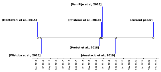
Figure 1: Timeline of related studies which perform automatic design of defaults hyperparameter values.

Table 1: Main characteristics of the “learning” task performed by related studies. Columns show for each related study: its reference, year of publication, ML algorithms studied, and the number/source of the datasets.

Reference	ML Algorithms	# Datasets	Data Source
			OpenML	UCI	AClib
[35]	SVM	145	$\bullet$	$\bullet$
[52]	SVM, AdaBoost	25		$\bullet$
[41]	SVM, kNN, CART,	38*	$\bullet$
	GBM, RF, Elastic-net
[40]	SVM, AdaBoost, CART,	38*	$\bullet$
	GBM, RF, Elastic-net
[45]	SVM	98	$\bullet$
[2]	Auto-WEKA	20			$\bullet$

*Only binary classification problems.

Table 2: Main characteristics of the “tuning’ task performed by related studies. Columns show for each related study: its reference, year of publication, tuning techniques explored, performance measures used, the evaluation methodology and baselines used in experimental comparisons.

Reference	Tuning	Performance	Evaluation	Baselines
	Techniques	Measures	Procedures
[35]	PSO	BAC	Nested-CV	WEKA defaults
			Outer: 10-CV	LibSVM defaults
			Inner: Holdout
[52]	NN-SMFO	Ranking	Nested-CV	SCoT, RS,
		CANE	Outer: 10-CV (outer)	SMAC ++
			Inner: Holdout	MKL-GP, RC-GP
[41]	SMBO	Accuracy, AUC	Single-CV	None
		$R^{2}$, Kendall’s tau	10-CV
[40]	RS	Accuracy	Nested-CV	None
	SMBO	AUC	Outer: 10-CV
			Inner: Holdout
[45]	GS	AUC	Single-CV	None
			10-CV
[2]	SMAC	Error rate	single-CV	Auto-WEKA defaults
	GGA++
	Irace

2.3.1 Our very first try on shared default settings

In [35], the authors used the Particle Swarm Optimization (PSO)algorithm to perform HP tuning of SVMs, and find new “default” hyperparameter settings for them. The optimization task was performed simultaneously with $21$ random datasets. The HP settings returned by the HP tuning task were considered as new “optimized default” HP settings. These values were compared to the default settings recommended in the Weka tool [21] and in the LibSVM library [17]. The experiments showed promising results whereby the new optimized settings induced models better than baselines for most of the investigated datasets.

2.3.2 Sequential Model-Free Hyperparameter Tuning

In [52], the authors proposed a method to select the best HP setting from a finite set of possibilities, which can be seen as a set of default HP settings. They used a Nearest Neighbor Sequential Model-Free Optimization (NN-SMFO)method to assess the average performance of an HP setting only on the $k$ datasets that were similar to the new test dataset. Two datasets are considered similar if they behave similarly, e.g., they have similar predictive performance rankings with respect to the HP settings. The authors claim that few evaluations are enough to approximate the true rank and that performance ranking is more descriptive than distance functions based on meta-features, i.e., features describing properties of a dataset, and construct the feature space for meta-learning. Experiments were performed with AdaBoost and SVMs using a set of 108 and 288 HP settings, respectively, generated from a grid of HP values. Besides converging faster than the other strategies, NN-SMFO also presented the smallest ranking and average normalized error. However, these gains were not validated by a statistical significance test. In addition, the coarse Grid Search (GS)used in the experiments was probably missing promising HP search space regions.

2.3.3 Tunability: Importance of Hyperparameters of Machine Learning Algorithms

[41] also defined default HP values empirically based on experiments with $38$ binary classification datasets. In their experiments, the best default HP setting is the configuration that minimizes on average a loss function considering many datasets, i.e., HP default settings are supposed to be suitable across different datasets. In the study, a set of HP settings is not directly evaluated due to the high computational cost. Instead, a surrogate regression model based on a meta-dataset is used. Thus, the surrogate model learns to map an HP setting to the estimated performance of a ML algorithm with respect to a dataset. The authors performed experiments with six ML algorithms, including DT induction, SVMs and gradient boosting. At the end, they analyzed the impact of tuning the algorithm and its HPs, namely tunability.

2.3.4 Learning Multiple Defaults for Machine Learning Algorithms

In [40], the authors wanted to find default values that generalize well for many datasets instead of only for specific datasets. In their experiments, they took advantage of a large database of prior empirical evaluations available on OpenML [50] to explore their hypothesis. Due to the high computational cost to estimate the expected risk of an induced algorithm using CV, surrogate models were used to predict the performance of the HP settings. Thus, any HP setting is evaluated faster using a surrogate model trained for each dataset. Finally, a greedy optimization technique searches through a list of defaults based on the predictions of the surrogate models. They assume that this list has at least one setting that is suitable for a given dataset. Experiments were carried out using 6 learning algorithms on a nested leave-one-out CV resampling method for up to 100 binary balanced datasets. According to the experimental results, a set of at most 32 new default settings outperformed two baseline strategies, RS and SMBO, for a budget size with 32 and 64 iterations, respectively. Therefore, new default settings are especially valuable when processing time is scarce to perform HP tuning.

Although the new default values are interesting from the practical point of view, this study was not concerned with the default values found and the characteristics of the datasets. Our current study overcomes this necessity to better understand the problem itself, which may be useful to the proposal of alternative default HP settings. HP tuning is usually performed by most of the methods starting from scratch for each dataset. If HP values are somehow dependent on dataset properties, this relation could be learned for a warm start of optimization methods [42, 22], for the prediction of HP values [20] or for the proposal of symbolic default HP settings [45].

2.3.5 Meta Learning for Default–Symbolic Defaults

Instead of searching for a good set of default HP values, [45] used meta-learning to learn sets of symbolic default HP settings suitable for many datasets. Symbolic default values are functions of the characteristics of the data rather than static values. An example of symbolic default is the relation to the number of features $n$ used by LibSVM to define the width ($gamma$) of the Gaussian kernel ($\gamma=1/N$) HP. Experiments were performed considering five different functions (transformations) over 80 meta-features for the $\gamma$ and $C$ of a SVM with Gaussian kernel. The experimental results showed that this technique is competitive to Grid Search (GS)using a surrogate model to predict the performance on a specific dataset. However, in this study, the authors only analyzed a symbolic default at each time when other HPs received static values, i.e., the authors did not take into account how multiple HPs could interact.

2.3.6 Importance of Default values for a warm-start HP tuning

Usually, algorithm configurators initialize their search for the best settings based on random values. An alternative for a warm-start is to take advantage of default settings. According to [2], default settings contain valuable information that can be exploited for HP tuning. Guided by this hypothesis, they investigated the benefit of using default settings for different automatic configurators, namely  SMAC [26], GGA++ [4], and Irace [10]. In addition, they proposed two simple methods to reduce the search space based on default values. The empirical analysis was performed considering 20 problems of AClib [27], including four datasets to evaluate Auto-WEKA, an automated searching system based on the WEKA learning algorithms and their HP settings. According to experimental results, default hyperparameter settings can critically influence on the configurators’ performance. This positive impact was observed mainly for Irace and other ML problems. Moreover, the methods to reduce the search space led to smaller error rates for the SMAC algorithm. Thereby, the authors claim that default hyperparameter settings provide valuable information for automated algorithm configuration.

2.4 Summary of Literature Overview

As previously mentioned, the literature review carried out for this study found only six studies investigating the generation of default HP settings for ML, each addressing a related issue, as discussed next:

• Three studies did not exactly perform HP tuning [52, 40, 41]: they “simulate” HP tuning via surrogate models. These surrogate models predict the expected performance for a given HP setting. The benefits of this approach are to set up the optimization process and reduce the cost associated with evaluating each single setting. On the other hand, they can propagate an erroneous value if the predictions are very different from the true predictive performance values;

• In [45], the authors try to induce new symbolic relationships between the datasets’ characteristics to set the HP values of an ML algorithm. In fact, they do not directly suggest a value, but a heuristic (formula) whose output depends on the dataset used;

• In [40], the authors propose a pool of default HP settings according to empirical data available on OpenML. There is also no tuning, just ranking and evaluation of prior HP settings. This technique might work in specific conditions, but it is not clear how these default values work for new datasets;

• In [2], the authors investigate the warm start of algorithm configuration tools, but the evaluation is focused on algorithm configuration problems (AClib).

3 Experiments

In this section we present an overview of the experimental strategy adopted to generate a pool of HP settings (Sec. 3.1), the datasets (Sec. 3.2), and the experiments carried out to evaluate this strategy (Sec. 3.3). Our hypothesis is that the HP settings generated by this strategy can lead to models with high predictive performance for datasets of different domains, and, therefore, can be considered as default values by a ML tool. The main purpose of providing such settings is to save users time, which can evaluate a small number of potential settings, instead of performing HP tuning for each new dataset under analysis, which is very time consuming.

3.1 Generating default HP settings

An overview of the experimental strategy followed to generate default HP settings is presented in Figure 2. Before explaining this strategy, we need to define some terms and choices:

• a target ML algorithm: the algorithm whose hyperparameter values will be optimized;

• an optimization technique: a technique that will conduct the optimization process;

• a sample of datasets: a set of datasets used to evaluate candidate solutions for new default HP settings; and

• an optimization criterion: a criterion that defines how candidate solutions will be evaluated and handled during the optimization.

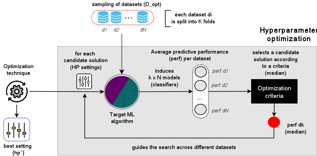
Figure 2: The proposed strategy to generate HP settings through an optimization process over datasets of different domains.

Since the search process is guided by the predictive performance of the models induced by a target algorithm, the proposed strategy will generate HP settings that are restrict to this algorithm. Although this process is computational costly, this is performed only once and the generated settings can be added in the ML tools as default values for this specific algorithm. Regarding the optimization technique, there is no restriction for this choice and, thus, any general purpose technique can be explored. However, considering that the goal is to generate a pool of HP settings, while population-based optimization algorithms are able to generate a pool of candidate solutions at once,other techniques, for the same purpose, need to be run multiple times. Additionally, this pool should be as diverse as possible, i.e., it is expected that these settings represent different regions of the search space.

With both target and optimization algorithms defined, a sample of datasets $D$ representing a wide range of different application domains has to be rigorously selected. In this case, it should be avoided to include, for instance, datasets that were created through data transformation processes from other datasets. These datasets are randomly split into two partitions, D_opt and D_test. The former partition is used during the HP optimization process to generate a pool of HP settings, while the latter is used to assess the predictive performance of the ML technique using these settings. This is very similar to a traditional holdout method, but instead of splitting the examples of a dataset, each instance is, itself, a dataset, named $d_{i}$.

In a traditional HP tuning design, the optimization technique is usually guided assessing the model’s predictive performance for different HP settings considering a specific dataset at hand. On the other hand, in the proposed strategy, for each candidate solution $h$ generated by the optimization technique, the target learning algorithm induces a model (classifier) for each dataset $d_{i}\in D_{opt}$ with $i=\{1,2,3,\ldots,N\}$. The predictive performance of each model is assessed by the stratified cross-validation method (perf $d_{i}$) and an appropriate measure. Based on these $N$ performances, the optimization technique uses a criterion, such as mean or median, to determine the fitness value of the candidate solution $h$.

At the end of the optimization process, one or more HP settings, which best performed, can be adopted by this strategy. E.g., if a population-based technique is used, either the best individual or the whole population could be considered. In addition, other variability factors could be explored to obtain a pool of settings, such as by choosing different subsets of $D_{opt}$.

3.2 Datasets

For the experiments carried out in this study, we used a dataset collection from the Open Machine Learning (OpenML)repository [50] that were curated by [36]. This collection has $156$ heterogeneous datasets, covering problems from different application domains, presenting different numbers of features, examples, and classes. From this set of datasets, the optimization process could not finish within the defined budget time (100 hours) for $6$ datasets. Therefore, in the present paper, $150$ datasets were used in the experiments. We considered preprocessing steps to enlarge the number of viable datasets in our experiments without affecting the results, since it occurred before any tuning procedure.

In order to be suitable for SVMs, all the datasets were preprocessed by:

• Removing constant and identifier features;

• Converting logical (boolean) attributes into numeric values $\in\{0,1\}$;

• Imputing missing values by the median in numerical attributes and a new category for categorical ones;

• Converting all the categorical features to numerical values using the 1-N encoding;

• Normalizing all the features with $\mu=0$ and $\sigma=1$.

After preprocessing the datasets, they were randomly split into two partitions, $D_{opt}$ and $D_{test}$, of equal sizes ($75$ datasets each). The datasets in $D_{opt}$ are used during the HP optimization process, while the effect of the settings in the predictive performance are assessed using the datasets in $D_{test}$. Since these partitions are defined at random, we repeated the sampling process five ($5$) times, to reduce the variance related to the dataset split [16]. This is similar to the 5x2 CV, but each instance of a partition represents a dataset itself, instead of an example.

We used the mlr [11] R package to preprocess the datasets. More information regarding datasets and the selection criteria can be found in [36]. Besides, a detailed list of these datasets can be found in our OpenML study page .

3.3 Optimization process

Although our strategy is suitable to generate a pool of new (default) HP settings for any ML algorithm, we decided to evaluate this strategy using SVM as the target algorithm due to its highly sensitive to HP tuning [7, 36], as confirmed by our literature review (see Table 2). Thus, new optimized default settings can be useful to avoid HP tuning and, consequently, reduce the computational cost of running these processes.

We selected the Particle Swarm Optimization (PSO)as the optimization technique [47] for these experiments. The literature has benchmarked different optimization techniques for SVM tuning [33]. However, they showed similar results when comparing the performance of their induced models. Among the tuning techniques reported, the PSO converged faster than the others, it did not require prior tuning, and was robust to obtain accurate HP settings in different types of datasets.

Another decision regarding the experimental strategy is the number of datasets $D_{opt}$ used in the optimization. The smaller the number of datasets, the less the computational time necessary to perform the HP optimization. Besides, there is not a strong assumption that the larger the number of datasets, the better the settings found, since it could prevent the diversity of HP settings. Thus, we investigated whether it is possible to obtain suitable settings with few datasets, and how the number of datasets affects the quality of these settings. For such, we evaluated $4$ (four) different sample sizes of $D_{opt}$, $S_{k}$, with $k=\{11,31,51,71\}$ datasets. The smallest sample considers just $11$ of the $75$ datasets in $D_{opt}$, while the largest sample, $S_{71}$, includes almost all the $D_{opt}$ datasets. It is important to mention that the smallest samples are contained in the largest samples, i.e., $S_{11}\subset S_{31}\subset S_{51}\subset S_{71}\subset D_{opt}$.

The optimization criterion used by the PSO to assess the fitness of a candidate solution $h$ is the median of the predictive performance of $h$ over all datasets in $S_{k}$ measured by the BAC measure. This centrality measure was chosen because it is less sensitive to outliers than the mean measure.

3.3.1 Hyperparameter space

The SVM HP space used in the experiments is presented in Table 3. For each HP, we show its symbol, name, and range or options of values. We only considered the Radial Basis Function (RBF)kernel in the experiment since: i) it achieves good performance values in general; ii) it may handle nonlinear decision boundaries, and iii) it can approximate the other kernel types [25]. The HP ranges shown in this table were first explored in [44].

Table 3: SVM hyperparameter space used in experiments. This table shows, for each hyperparameter, its symbol, name and range/options of values when tuned.

Symbol	Hyperparameter	Range/Options
k	kernel	{RBF}
C	cost	$[2^{-15},2^{15}]$
$\gamma$	width of the kernel	$[2^{-15},2^{15}]$

3.3.2 Experimental setup

We present the complete experimental setup in Table 4. Since PSO is a stochastic method, we executed it $10$ times with different seeds for each sample $S_{k}$, with a population of $10$ particles and a budget of $300$ iterations or $100$ hours. The number of evaluations was defined by prior experiments with HP tuning evaluation [34]. The initial population was warm-started with the defaults from WEKA ($Cost=1$, $\gamma=0.01$). To assess the models’ performance in the fitness function, we used a single stratified Cross-validation (CV)resampling method with $10$ folds. Only the particle (solution) with the best fitness is included in the pool of default HP settings.

Therefore, in our experimental setup, the proposed strategy is generating a pool of $50$ HP settings for each sample size $S_{k}$. This number is due to the 10 repetitions of PSO times 5 replications of the sampling method ($5\times 2$ CV, Sec. 3.2). Only the best particle of each PSO repetition is included in the pool.

To evaluate these $50$ settings, every HP setting in this pool is assessed for every dataset in $D_{test}$, selecting the best setting per dataset, i.e., the HP setting that induced the model with the highest predictive performance. The results of this evaluation are hereafter referred to as “default.opt” (default optimized HP), or “def.opt” for short. We compared default.opt with two baselines:

1. Defaults from ML tools (lower bound): default HP values from mlr (LibSVM/R), Weka (Java) and scikit-learn (Python) software/packages; and

2. Conventional HP tuning (upper bound): HP tuning results of an RS technique performed on each dataset with the same budget (300 evaluations). RS proved to be competitive for SVM assessment [7, 34], inducing models as accurate as those induced by more robust techniques (SMBO, PSO, EDA).

The predictive performance of the proposed strategy and the baselines are assessed by the BAC measure for the test datasets $D_{test}$ and the $10$-fold stratified CV resampling procedure. It is important to note that the HP settings suggested by default.opt and RS were estimated using $D_{opt}$ and assessed in $D_{test}$, which are mutually exclusive (Section 3.2).

Hence, the tuning setup detailed in Table 4 were executed by parallelized jobs in a cluster facility and it took one month to be completed. The PSO algorithm was implemented in R using the pso package. The code developed for this study is also hosted at GitHub . There, one can find the optimization jobs and the automated graphical analyses.

Table 4: Hyperparameter tuning experimental setup.

Element	Feature	Value	R package
HP tuning	Technique	Particle Swarm Optimization	pso
	Stopping criteria	budget size
	Population size	10
	Maximum number of iterations	30
	Budget size	300
	fitness criteria	median
	Algorithm implementation	SPSO20071
Target algorithm	ML algorithm	Support Vector Machines	e1071
Sample size	Number of datasets	{11, 31, 51, 71}
Resampling Strategy	Single Loop	Cross-validation (CV)	mlr
		10-fold
Performance measures	Optimized (fitness)	Balanced per class accuracy	mlr
	Evaluation	{Balanced per class accuracy,
		optimization paths}
Repetitions	Seeds	10 values
		seeds = $\{1,\ldots,10\}$
Baselines	Default settings	LibSVM2	e1071
		WEKA3	RWeka
		Scikit-learn4	-
	Tuning	Random Search	mlr

1 - Implementation detailed in [18].

2 - https://cran.r-project.org/web/packages/e1071/e1071.pdf

3 - https://weka.sourceforge.io/doc.dev/weka/classifiers/functions/SMO.html

4 - https://scikit-learn.org/stable/modules/generated/sklearn.svm.SVC.html

4 Results and Discussion

In this section, we present and discuss the main experimental results obtained using the proposed strategy to generate a pool of default HP settings. An overall analysis, including the comparison of the proposed strategy with the baselines, is introduced in Section 4.1, while a detailed assessment of these achievements and the optimized default settings found by our strategy are presented in Sections 4.2 and  4.3, respectively. How these results could help us to better understand whether or not HP tuning should be performed for a give problem is investigated in Section  4.4. All these results refer to the pool of HP settings using the sample size $k=51$, which led to the models with the highest predictive performance. Finally, we discuss and analyze the sensitivity of our strategy to different sample sizes in Section 4.5.

4.1 Optimized default settings

The results considering all strategies for setting SVM HP, including default.opt with sample size $k=51$, are presented in Figure 4 (see Appendix F for other sample sizes). The violin plots show the distribution of the BAC values (x-axis) obtained by these strategies (y-axis) across all datasets in $D_{test}$, sorted accordingly to their average performance. The vertical red dotted line represents the median value obtained by default.opt strategy and is used to highlight differences for the baselines. Comparing the strategies, the best results were obtained by the RS technique (0.719), with a small difference to the optimized default settings (0.706). Default HP settings from different ML tools presented a very similar distribution and the same performance (0.644), which is worse than that of default.opt.

The Friedman test was applied to assess the statistical significance of the HP strategies considering a significance level of $\alpha=0.05$ [46]. The null hypothesis states that all the strategies have equivalent predictive performance. When the null hypothesis is rejected, the Nemenyi post-hoc test is also used to indicate which strategies are significantly different.

Figure 4 presents the resultant Critical Difference (CD)diagram. In this diagram, strategies are connected when there are no significant differences between them. Therefore, according to this test, there is no significant difference between RS and the new optimized settings (default.opt). It is important to highlight that, in spite of its simplicity, RS optimizes the HP values for each dataset, evaluating a high number of candidate solutions. Thus, its computational cost is much higher than the cost of evaluating the pool of the settings obtained by the proposed strategy, default.opt. In summary, these results show that default.opt is able to find appropriate HP settings since it outperformed the ML tools and was competitive with RS.

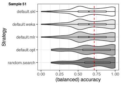
Figure 3: BAC performance distributions obtained by different strategies evaluated in the test datasets and default.opt with $k=51$.

Figure 4: The CD diagram considering the BAC values of the HP settings found by different strategies (default.opt with $k=51$) for SVMs according to the Frideman-Nemenyi test ($\alpha=0.05$). Groups of strategies that are not significantly different are connected.

4.2 Improvement Analysis

For a more in-depth analysis of the improvements achieved by our strategy, Figure LABEL:fig:svm_agg_improvements shows the BAC values (y-axis) for each dataset (x-axis) averaged over the 5x2 CV resampling results. Different colors and shapes of lines represent different HP strategies. These datasets are named by their OpenML IDs and are listed by decreasing BAC values obtained by default.mlr (LibSVM).

Figure LABEL:fig:svm_agg_improvements shows that default HP settings from ML tools (mlr, Weka and scikit-learn) performed similarly for all datasets, what was expected given the overall analysis, and, thus, their curves were usually overlapped. The new optimized HP settings (red line), generated by our strategy, and the RS technique (blue line) outperformed them in most of the datasets. This figure also shows that the behavior of the default.opt’s curve is very similar to the RS curve, including the cases of performance gains. Our initial hypothesis was that RS would defeat the new optimized default settings. Thus, this achievement is surprising to some extent given that RS is performing HP tuning for each dataset, and is consequently much more time consuming when compared to the few evaluations needed to evaluate a small set of optimized settings.

The Wilcoxon paired-test (with $\alpha=0.05$) was applied to assess the statistical significance of the results between the two best-ranked HP strategies per dataset considering the averaged BAC values presented in Figure LABEL:fig:svm_agg_improvements. Table 5 presents the frequency each strategy was best ranked with (p-value $<0.05$) and without (p-value $\geq 0.05$) statistical significance when compared to the second best strategy. The comparison RS vs Tools only considers defaults from the ML tools whereas RS vs All also considers the optimized defaults.

Table 5: Wilcoxon paired test comparing the two best HP strategies ranked by data set. For each HP strategy, the frequency with which it was ranked first with (p-value $<$ 0.05) and without (p-value $\geq$ 0.05) statistical significance is presented. Table presents aggregated results for all the different test sets used.

Strategy	RS vs Tools		RS vs All
	$<0.05$	$\geq 0.05$	$<0.05$	$\geq 0.05$
Random Search (RS)	89	37	38	45
Default opt	–	–	10	43
Default mlr	0	15	0	10
Default skl	0	9	0	4
Default Weka	0	0	0	0
Total of test cases	150		150

Overall, the RS technique significantly outperformed ($<0.05$) default settings from tools in $89$ datasets. For the remaining ($\geq 0.05$), there was no significant difference among RS and tools, but the former was ranked as the first strategy for $37$ out of $61$ datasets. Therefore, HP tuning is recommended for these $89$ datasets, since in practice, due to its computational cost, we would employ it just when it is likely to significantly improve predictive performance. Some studies, such as [36], showed that it is possible to predict with high accuracy whether or not a process of HP tuning is necessary for the dataset under analysis. When the default optimized settings are included in this comparison (RS vs All), they were able to remarkably reduce the number of datasets where RS is recommended to $38$ ($<0.05$). Besides, optimized defaults were significantly better than the second ranked strategy for $10$ cases. Thus, using the method proposed by [36], the HP tuning would be performed on only $38$ datasets, instead of $89$.

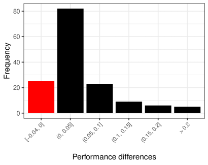
Figure 5: Performance differences in terms of BAC when comparing results obtained by the default optimized HP settings to the defaults from ML tools.

In order to compare the pool of optimized default HP settings with those provided by the ML tools, Figure 5 shows the distribution of the predictive performance difference assessed by BAC values for all datasets. Black bars represent favorable differences to our strategy (positive differences indicate improvement) whereas red bars indicate when traditional defaults were better (negative differences). Observing the red bar, one can notice the traditional defaults only achieved minimal advantages since they are mostly close to zero. On the other hand, when using the new optimized HP settings, there are cases with medium (between $0.05$ and $0.1$) and high improvement (above $0.1$).

4.3 Analysis of the new optimized SVM HP values

Figure 6 depicts the dispersion of the new optimized HP settings in the SVM HP space. The x-axis shows the cost (C) values and the y-axis shows the gamma ($\gamma$) values, both in the $log_{2}$ scale. Different shapes and colors denote HP settings obtained considering the five different $D_{opt}$ sets. The dashed circle indicates the region containing the HP values included in the initial population of the optimization method.
In addition, the black cross and the blue point represent default values from ML tools in datasets where our strategy performed best and worst, respectively.

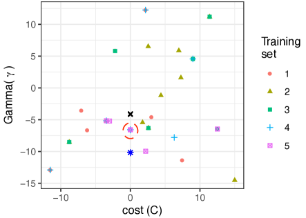
Figure 6: The dispersion of the new optimized HPs settings obtained with sample size $k=51$. Values projected on the $log_{2}$ scale. The black cross and blue point shows default values from ML tools in datasets where our strategy performed best and worst, respectively.

Table 6: Top-ranked HP settings obtained with shared optimization and sample size = 51. Values are represented in $log_{2}$ scale.

Rank	HP Setting
	Cost (C)	Gamma ($\gamma$)
1	-2.1927	5.7930
2	3.0154	-4.5968
3	8.9897	4.5561
4	0.0000	-6.6000
5	12.5062	-6.4680
6	7.4370	-11.4271
7	-7.0694	-3.5971
8	-6.1878	-6.6787
9	-11.5290	-12.9075
10	2.1856	12.2462

According to this figure, there is a dispersion of the new optimized HP settings across the hyperspace. Besides, different training sets influenced the optimization process differently, with their HP settings located in different regions:

• Training sets 1, 2, 3, 4: these were able to generate various HP settings across the investigated datasets. Their HP values differ from traditional defaults. Thus, the search explored different regions from the space, and these different settings were able to induce models with good performance, often better than traditional defaults;

• Training set 5: provided few variability on their optimized settings, with most of them placed near the initial search space. Thus, one may argue that optimization became stuck in a local minimum, considering those datasets, and did not explore the remainder of the space. Nevertheless, even with values closer to the traditional ML defaults, they were competitive to the RS baseline, as shown in Figure LABEL:fig:svm_agg_improvements and Table 5.

The top-ranked HP settings obtained by the optimization average over all test sets ($D_{test}$) are presented in Table 6. Appendix C presents an extended table with all the unique HP settings we obtained in our experiments with the best experimental setup (sample size $k=51$).

4.4 Learning from new optimized defaults

Although the strategy to find optimized default settings works well, some questions regarding its use may arise. For example, “what both dataset and learning characteristics can tell us about when to use the pool of optimized HP settings instead of a tuning technique, such as RS?”. The answer to this question can help users to choose between either HP tuning, which can provide better settings but is computationally expensive, or testing a set of default HP values. Moreover, finding some patterns regarding this task may bring some knowledge about the learning process.

Here, we borrow some ideas from Meta-learning (MtL) [31] to investigate this problem as a binary classification task where classes identify whether the pool of default optimized HP settings are sufficient for a given dataset or HP tuning using RS should be performed. HP tuning is recommended when it significantly outperformed the new default HP settings for a given dataset based on the Wilcoxon test, previously discussed in Section 4.2. The predictive attributes consist of different characteristics extracted from each dataset using the pymfe(v0.4) tool, with the mean (nanmean) and standard deviation (nanstd) summary functions [1].

Figure 7: BAC of the LOO-CV using simple and general meta-feature groups with the sample size $k=51$.

We considered in our analysis each test set, and the average of these sets for the sample size $k=51$. The data generated for each one was used by the Decision Tree (DT)and Random Forest (RF)algorithms to induce predictive models. These algorithms were selected because they can induce explainable models, and are therefore able to shed some light on the learning process. Due to the presence of class imbalance in the meta-dataset, we also included an RF version that deals with imbalance (Bal-RF), a DT performing oversampling via SMOTE, and cleaning using ENN (Smoteenn). These ML and preprocessing algorithms are available in the scikit-learn and imbalanced-learn Python libraries [30, 39]. Their results were compared with a baseline model that always predicts the majority class.

Figure 7 shows the BAC of the Leave-one-out Cross-validation (LOO-CV)(y-axis) considering only simple and general descriptors for each test set and their average. In this figure, different algorithms are represented by different colors, line types and shapes. Overall, the best result was obtained by the DT algorithm with a BAC of $0.72$ for the third test set, which is $0.19$ higher than the baseline, suggesting that this algorithm could learn some patterns from these data. On the other hand, the induced models did not overcome the baseline for some test sets, which may be an indicator that we have a difficult learning problem.

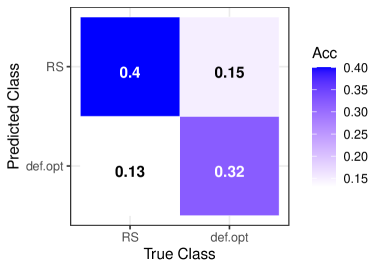
Figure 8: Confusion matrix of the best induced DT model (0.72) in test set 3, with general and simple descriptors and not using the Smoteenn.

Figure 8 shows the confusion matrix for the best DT model. The difference between the accuracies for each class indicates that this model is more prone to hit the RS class than the def.opt class. This behavior is desired when predictive performance is the main concern, since it spends more computational time performing hp tuning but avoid performance loss.

Although we have shown that these models are better than a guess, we have no access to which characteristics make a dataset more prone to RS than to the pool of optimized HP yet. Therefore, we draw the best DT model to understand the learned patterns. Due to its size, the complete DT model is presented in Appendix E. There, we present the entire DT model, its branches, leaves, the yielded rules, and a histogram of the features.

Based on this model, we can observe two interesting rule paths where more than half of the dataset is included. The first rule is shown next, where $20$ out of the $23$ examples (datasets) are from the default.opt class and the remaining $3$ examples are from the rs class. This rule evaluates the number of instances from a dataset (nr_inst), the total number of attributes (nr_attr) and the proportion of these two characteristics, i.e., the number of attributes divided by the number of instances (attr_to_instance). This rule suggests that optimized HP settings are more suitable for datasets with a small number of examples ($<358$) and attributes ($<88$). It may be motivated by the nature of most of datasets presented in the UCI and OpenML repositories, mostly ”simple’ problems.

     nr_inst < 358    attr_to_instance >= 0.02        nr_attr < 88            [20/3] (default.opt/RS)     

The second interesting rule path has $28$ examples, $24$ from the RS class and $4$ from the default.opt class. This rule suggests that the tuning process should be performed for datasets with more examples (nr_inst $\geq 358$) and balanced classes (with a standard deviation of the relative frequency of each class $\geq 0.43$). Overall, the induced tree presents interesting patterns by using simple dataset characteristics. Moreover, as this tree is small, the practitioners can use it to identify when to use default settings or perform HP tuning for their new problems.

     nr_inst >= 358    freq_class.nansd >= 0.43        freq_class.nanmean >= 0.15            [4/24] (default.opt/RS)     

4.5 Sample Size Sensitivity Analysis

In the previous sections, we analyzed how suitable are the HP settings found by the proposed strategy considering the best sample size studied ($k=51$). In this section, we analyze how this strategy behaves for different sample sizes, i.e., we investigate the effect of the sample size in the HP settings starting with few datasets and increasing it until almost all training datasets ($D_{train}$) are used: $k={11,31,51,71}$.

Figure 10 shows the average BAC achieved by default.opt and the baselines. This figure suggests that our strategy is benefiting from bigger sample sizes, i.e., $k=\{51,71\}$ datasets, when there is a clear approximation to the RS and a larger distance to the defaults of ML tools. Even with the average values attenuating their differences and with a high standard deviation (shaded colors), both cases show a promising scenario.

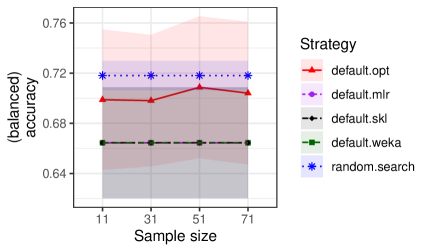
Figure 9: Mean BAC performance values evaluated in test datasets with different sample sizes.

Figure 10: Comparison of the BAC values of the different HP settings according to the Friedman-Nemenyi test ($\alpha=0.05)$ for different sample sizes.

To confirm whether these sample sizes yielded different performances, we also applied the Friedman test with a significance level $\alpha=0.05$. The null hypothesis states that all the sample sizes are equivalent with respect to the Balanced per class Accuracy (BAC)values. Figure 13 presents the resultant Critical Difference (CD)diagram. The smallest sample ($k=11$) was statistically worse than sample sizes $k=\{51,71\}$. In all the remaining cases, there is no significant differences despite the bigger difference between $k=\{31\}$ and $k=\{51,71\}$. This analysis suggests that smaller samples are less appropriate. However, although we did not have statistical evidence to choose a sample size among $k=\{31,51,71\}$, we chose the best one ($k=\{51\}$) for the previous experimental analysis.

In the proposed strategy, the fitness value to find default optimized settings considers the predictive performance across different datasets (see Fig. 2). Thus, one could argue that the higher the number of datasets used in this process the better the HP settings found, and, consequently, the predictive performance. This probably would be true if we had considered only the best setting. Instead, we are interested in analyzing a pool of settings. Thus, there is a trade-off between the sample size and the diversity, i.e., smaller sample sizes are more likely to generate settings that cover different regions of the search space.

5 Threats to Validity

In an empirical study design, methodological choices may impact the results obtained in the experiments. Next, we discuss the threats that may impact the results of this study.

5.1 Internal validity

The datasets used in the experiments were preprocessed to be handled by SVMs. We also ensured that all classes in the datasets must have at least $10$ observations. Thus, 10-fold stratification can be applied without any concerns. Of course, other datasets may be used to expand data collection, if they comply with the ‘stratified’ criterion. However, the authors believe that adding datasets will not substantially change the overall behavior of HP strategies on the algorithm investigated, since they were selected to cover a wide range of classification tasks with different characteristics.

[28] compared different resampling strategies for assessing the predictive performance and selecting regression/classification models induced by ML algorithms. In [16], the authors also discuss the overfitting in the evaluation methodologies when assessing ML algorithms. Based on their discussion, the most reasonable choice for our experiments is the 5 times 2-CV resampling methodology. It is suggested for cases when it is desired to reduce the variance of the results generated using a dataset with few instances. It is exactly our case: we have a few instances ($150$) which are datasets feeding an optimization process. Thus, to reduce the bias of the performance evaluation and the computational cost of experiments, this resampling methodology was adopted in the experiments.

Since a wide variety of datasets compose the data collection, some of them may be imbalanced. Thus, the BAC measure [15] was used to assess the predictive performance of the models during the optimization process, i.e., in the fitness function. This measure considers class distributions when assessing the performance of a candidate solution. We used the same performance measure to evaluate the final solutions returned by the HP strategies. Other predictive performance measures can generate different results, depending on how they deal with data imbalance.

5.2 Conclusion validity

Section 4 presented statistical comparisons between the investigated tuning strategies. In [19], the author discusses the issue of statistical tests for comparisons of several techniques on multiple datasets, reviewing several statistical methodologies. The method proposed as more suitable is the non-parametric analog version of ANOVA, i.e., the Friedman test, along with the corresponding Nemenyi post-hoc test. The Friedman test ranks all the methods separately for each dataset and uses the average ranks to test whether all techniques are equivalent. In case of differences, the Nemenyi test performs all the pairwise comparisons between the techniques and identifies the presence of significant differences. Thus, the Friedman ranking test followed by the Nemenyi post-hoc test was used to evaluate our experimental results.

5.3 External validity

The experimental methodology described in Section 3 considers using HP tuning techniques that have been used and discussed in the literature, such as [40, 45]. The PSO and RS techniques were also exhaustively benchmarked for SVM tuning [33]. In the experiments carried out in this paper, we used the default settings provided by the PSO R implementation. These default values are robust for our dataset collection. Otherwise, the tuning of PSO would considerably increase the experimental cost by adding a new level of tuning (the tuning of tuning techniques). Thus, this additional level was not assessed in this study.

Using budgets for SVMs tuning was investigated in [34]. The experimental results suggested that all the considered techniques required only $\approx$ $300$ evaluations to converge. Convergence here means the tuning techniques could not improve their predictive performance more than $10^{-5}$ until the budget was consumed. Actually, in most cases, the tuning reached its maximum performance after $100$ steps. Thus, a budget size of $300$ evaluations was therefore deemed sufficient. Results obtained from this budget showed that the exploration made in hyperparameter spaces led to statistically significant improvements in most cases. Thus, this budget size was adopted in our experiments.

In this paper, we investigated a single ML algorithm. The methodology described here can be generalized to other ML algorithms, especially those that are sensitive to tuning. On the other hand, algorithms such as the RF whose defaults are robust enough [41] would not benefit from the new strategy. Nonetheless, additional similar studies may prove fruitful. For such, all the experimental data generated in the experiments are available at OpenML and GitHub.

6 Conclusion

The present paper proposes and rigorously analyzes a strategy to generate optimized HP settings for ML algorithms. This strategy was conceived from the observation that a limited number of default HP values is provided by most of the ML tools. Therefore, alternative default settings could improve model predictive performance besides reducing the need to perform HP tuning, which is a very time-consuming task.

For such, we carried out experiments adopting Support Vector Machines (SVMs)as the ML algorithm due to its sensitivity to HP tuning and used a collection of $150$ datasets carefully curated from the public repository OpenML. In addition, the PSO optimization technique was used to find HP settings that are appropriate for a sample of this collection of datasets.

Using this new set of HP values, referred to as default optimized, led to significantly better models than the defaults suggested by ML tools in all scenarios investigated. Furthermore, the optimized default settings were able to considerably reduce the number of datasets for which it is necessary to perform HP tuning. A sensitivity analysis of the strategy regarding sample size suggested there is a trade-off between finding robust HP settings, what requires a high number of datasets, and promoting diversity, using a smaller sample. In our experiments, the best results were obtained with a sample of $51$ datasets.

The ideal situation would be that where we could define for which problems default settings are sufficient and for which ones the HP tuning is indicated. Thus, we conducted experiments using characteristics extracted from the dataset collection and tree-based algorithms to provide some interpretability of the identified patterns. In our analysis, two main rules could be observed: (i) default optimized settings is a better option when a dataset has a small number of examples and attributes; and (ii) HP tuning is usually recommended for datasets with more examples and balanced classes. The robustness of these new optimized HP settings goes toward what has been discussed in the literature [7, 36, 51].

6.1 Main difficulties

The main difficulties faced during this study are related to the cost of the performed experiments. The optimization process is computationally expensive, since a large number of datasets are evaluated for every new candidate solution (HP setting). We also needed to run several rounds of experiments to calibrate our methodology, and each of these rounds took almost two months.

Another adversity is related to the data collection. Initially, a larger number of datasets were selected, but some of them presented problems when inducing SVMs models. Therefore, we preferred to not consider them in the experiments.

6.2 Future Work

The findings from this study open up future research directions. In the context of AutoML, the obtained HP settings can be used as a warm start for the optimization techniques. Moreover, instead of creating pipelines from scratch, the AutoML systems can create entire pipelines based only on the optimized defaults.

It would also be a promising direction to investigate different ways of coding the individuals in the optimization process. The sample size and correspondent datasets could be embedded in the candidate solution, along with the HP values, releasing designers from these empirical choices.

Another possibility would be to cluster the datasets according to their similarities to generate better-optimized HP values for each group. The fitness value used in the experiments is an aggregate measure of performance across different datasets. It would be interesting to explore other measures, such as average ranks.

The code used in this study is publicly available, easily extendable, and may be adapted to cover several other ML algorithms. Thus, experiments with different ML algorithms can also be carried out, investigating their HP profile: the need for tuning, how defaults behave, and so on. All the information generated can also be used as meta-knowledge to feed further experiments.

Appendix A List of abbreviations used in the paper

Appendix B List of datasets used in the experiments

Table 7: (Multi-class) classification OpenML datasets (1 to 43) used in experiments. It is shown, for each dataset: the OpenML dataset name and id, the number of attributes (D), the number of examples (N), the number of classes (C), the number of examples belonging to the majority and minority classes (nMaj, nMin), and the proportion between them (P).

Nro	OpenML name	OpenML did	D	N	C	nMaj	nMin	P
1	kr-vs-kp	3	37	3196	2	1669	1527	0.91
2	breast-cancer	13	10	286	2	201	85	0.42
3	mfeat-fourier	14	77	2000	10	200	200	1.00
4	breast-w	15	10	699	2	458	241	0.53
5	mfeat-karhunen	16	65	2000	10	200	200	1.00
6	mfeat-morphological	18	7	2000	10	200	200	1.00
7	car	21	7	1728	4	1210	65	0.05
8	mfeat-zernike	22	48	2000	10	200	200	1.00
9	colic	25	28	368	2	232	136	0.59
10	optdigits	28	65	5620	10	572	554	0.97
11	credit-g	31	21	1000	2	700	300	0.43
12	pendigits	32	17	10992	10	1144	1055	0.92
13	dermatology	35	35	366	6	112	20	0.18
14	segment	36	20	2310	7	330	330	1.00
15	diabetes	37	9	768	2	500	268	0.54
16	sick	38	30	3772	2	3541	231	0.07
17	sonar	40	61	208	2	111	97	0.87
18	haberman	43	4	306	2	225	81	0.36
19	spambase	44	58	4601	2	2788	1813	0.65
20	tae	48	6	151	3	52	49	0.94
21	heart-c	49	14	303	5	165	0	0.00
22	tic-tac-toe	50	10	958	2	626	332	0.53
23	heart-statlog	53	14	270	2	150	120	0.80
24	vehicle	54	19	846	4	218	199	0.91
25	hepatitis	55	20	155	2	123	32	0.26
26	vote	56	17	435	2	267	168	0.63
27	ionosphere	59	35	351	2	225	126	0.56
28	waveform-5000	60	41	5000	3	1692	1653	0.98
29	iris	61	5	150	3	50	50	1.00
30	molecular-biology_promoters	164	59	106	2	53	53	1.00
31	satimage	182	37	6430	6	1531	625	0.41
32	baseball	185	18	1340	3	1215	57	0.05
33	wine	187	14	178	3	71	48	0.68
34	eucalyptus	188	20	736	5	214	105	0.49
35	Australian	292	15	690	2	383	307	0.80
36	satellite_image	294	37	6435	6	871	275	0.32
37	libras_move	299	91	360	11	24	11	0.46
38	vowel	307	13	990	11	90	90	1.00
39	mammography	310	7	11183	2	10923	260	0.02
40	oil_spill	311	50	937	2	896	41	0.05
41	yeast_ml8	316	117	2417	2	2383	34	0.01
42	hayes-roth	329	5	160	4	65	0	0.00
43	monks-problems-1	333	7	556	2	278	278	1.00

Table 8: (Multi-class) classification OpenML datasets (44 to 88) used in experiments. For each dataset it is shown: the OpenML dataset name and id, the number of attributes (D), the number of examples (N), the number of classes (C), the number of examples belonging to the majority and minority classes (nMaj, nMin), and the proportion between them (P).

Nro	OpenML name	OpenML did	D	N	C	nMaj	nMin	P
44	monks-problems-2	334	7	601	2	395	206	0.52
45	monks-problems-3	335	7	554	2	288	266	0.92
46	SPECT	336	23	267	2	212	55	0.26
47	grub-damage	338	9	155	4	49	19	0.39
48	synthetic_control	377	62	600	6	100	100	1.00
49	analcatdata_boxing2	444	4	132	2	71	61	0.86
50	analcatdata_boxing1	448	4	120	2	78	42	0.54
51	analcatdata_lawsuit	450	5	264	2	245	19	0.08
52	irish	451	6	500	2	278	222	0.80
53	analcatdata_broadwaymult	452	8	285	7	118	21	0.18
54	cars	455	9	406	3	254	73	0.29
55	analcatdata_authorship	458	71	841	4	317	55	0.17
56	analcatdata_creditscore	461	7	100	2	73	27	0.37
57	backache	463	33	180	2	155	25	0.16
58	prnn_synth	464	3	250	2	125	125	1.00
59	schizo	466	15	340	2	177	163	0.92
60	analcatdata_dmft	469	5	797	6	155	123	0.79
61	profb	470	10	672	2	448	224	0.50
62	analcatdata_germangss	475	6	400	4	100	100	1.00
63	biomed	481	9	209	2	134	75	0.56
64	rmftsa_sleepdata	679	3	1024	4	404	94	0.23
65	visualizing_livestock	685	3	130	5	26	26	1.00
66	diggle_table_a2	694	9	310	9	41	18	0.44
67	ada_prior	1037	15	4562	2	3430	1132	0.33
68	ada_agnostic	1043	49	4562	2	3430	1132	0.33
69	jEdit_4.2_4.3	1048	9	369	2	204	165	0.81
70	pc4	1049	38	1458	2	1280	178	0.14
71	pc3	1050	38	1563	2	1403	160	0.11
72	mc2	1054	40	161	2	109	52	0.48
73	mc1	1056	39	9466	2	9398	68	0.01
74	ar4	1061	30	107	2	87	20	0.23
75	kc2	1063	22	522	2	415	107	0.26
76	ar6	1064	30	101	2	86	15	0.17
77	kc3	1065	40	458	2	415	43	0.10
78	kc1-binary	1066	95	145	2	85	60	0.71
79	kc1	1067	22	2109	2	1783	326	0.18
80	pc1	1068	22	1109	2	1032	77	0.07
81	pc2	1069	37	5589	2	5566	23	0.00
82	mw1	1071	38	403	2	372	31	0.08
83	jEdit_4.0_4.2	1073	9	274	2	140	134	0.96
84	datatrieve	1075	9	130	2	119	11	0.09
85	PopularKids	1100	11	478	3	247	90	0.36
86	teachingAssistant	1115	7	151	3	52	49	0.94
87	badges2	1121	12	294	2	210	84	0.40
88	pc1_req	1167	9	320	2	213	107	0.50

Table 9: (Multi-class) classification OpenML datasets (89 to 134) used in experiments. For each dataset it is shown: the OpenML dataset name and id, the number of attributes (D), the number of examples (N), the number of classes (C), the number of examples belonging to the majority and minority classes (nMaj, nMin), and the proportion between them (P).

Nro	OpenML name	OpenML did	D	N	C	nMaj	nMin	P
89	MegaWatt1	1442	38	253	2	226	27	0.12
90	PizzaCutter1	1443	38	661	2	609	52	0.09
91	PizzaCutter3	1444	38	1043	2	916	127	0.14
92	CostaMadre1	1446	38	296	2	258	38	0.15
93	CastMetal1	1447	38	327	2	285	42	0.15
94	PieChart1	1451	38	705	2	644	61	0.09
95	PieChart2	1452	37	745	2	729	16	0.02
96	PieChart3	1453	38	1077	2	943	134	0.14
97	acute-inflammations	1455	7	120	2	70	50	0.71
98	appendicitis	1456	8	106	2	85	21	0.25
99	artificial-characters	1459	8	10218	10	1416	600	0.42
100	banknote-authentication	1462	5	1372	2	762	610	0.80
101	blogger	1463	6	100	2	68	32	0.47
102	blood-transfusion-service-center	1464	5	748	2	570	178	0.31
103	breast-tissue	1465	10	106	6	22	14	0.64
104	cnae-9	1468	857	1080	9	120	120	1.00
105	fertility	1473	10	100	2	88	12	0.14
106	first-order-theorem-proving	1475	52	6118	6	2554	486	0.19
107	ilpd	1480	11	583	2	416	167	0.40
108	lsvt	1484	311	126	2	84	42	0.50
109	ozone-level-8hr	1487	73	2534	2	2374	160	0.07
110	parkinsons	1488	23	195	2	147	48	0.33
111	phoneme	1489	6	5404	2	3818	1586	0.42
112	qsar-biodeg	1494	42	1055	2	699	356	0.51
113	qualitative-bankruptcy	1495	7	250	2	143	107	0.75
114	ringnorm	1496	21	7400	2	3736	3664	0.98
115	wall-robot-navigation	1497	25	5456	4	2205	328	0.15
116	sa-heart	1498	10	462	2	302	160	0.53
117	steel-plates-fault	1504	34	1941	2	1268	673	0.53
118	thoracic-surgery	1506	17	470	2	400	70	0.18
119	twonorm	1507	21	7400	2	3703	3697	1.00
120	wdbc	1510	31	569	2	357	212	0.59
121	heart-long-beach	1512	14	200	5	56	10	0.18
122	robot-failures-lp4	1519	91	117	3	72	21	0.29
123	robot-failures-lp5	1520	91	164	5	47	21	0.45
124	vertebra-column	1523	7	310	3	150	60	0.40
125	volcanoes-a2	1528	4	1623	5	1471	29	0.02
126	volcanoes-a3	1529	4	1521	5	1369	29	0.02
127	volcanoes-b1	1531	4	10176	5	9791	26	0.00
128	volcanoes-b3	1533	4	10386	5	10006	25	0.00
129	volcanoes-b5	1535	4	9989	5	9599	26	0.00
130	volcanoes-b6	1536	4	10130	5	9746	26	0.00
131	volcanoes-d2	1539	4	9172	5	8670	56	0.01
132	volcanoes-d3	1540	4	9285	5	8771	58	0.01
133	autoUniv-au1-1000	1547	21	1000	2	741	259	0.35
134	autoUniv-au6-750	1549	41	750	8	165	57	0.35

Table 10: (Multi-class) classification OpenML datasets (135 to 150) used in experiments. For each dataset it is shown: the OpenML dataset name and id, the number of attributes (D), the number of examples (N), the number of classes (C), the number of examples belonging to the majority and minority classes (nMaj, nMin), and the proportion between them (P).

Nro	OpenML name	OpenML did	D	N	C	nMaj	nMin	P
135	autoUniv-au6-400	1551	41	400	8	111	25	0.23
136	autoUniv-au7-1100	1552	13	1100	5	305	153	0.50
137	autoUniv-au7-500	1554	13	500	5	192	43	0.22
138	acute-inflammations	1556	7	120	2	61	59	0.97
139	bank-marketing	1558	17	4521	2	4000	521	0.13
140	breast-tissue	1559	10	106	4	49	14	0.29
141	hill-valley	1566	101	1212	2	612	600	0.98
142	wilt	1570	6	4839	2	4578	261	0.06
143	SPECTF	1600	45	267	2	212	55	0.26
144	PhishingWebsites	4534	31	11055	2	6157	4898	0.80
145	cylinder-bands	6332	40	540	2	312	228	0.73
146	cjs	23380	36	2796	6	576	341	0.59
147	thyroid-allbp	40474	27	2800	5	1632	31	0.02
148	thyroid-allhyper	40475	27	2800	5	1632	31	0.02
149	LED-display-domain-7digit	40496	8	500	10	57	37	0.65
150	texture	40499	41	5500	11	500	500	1.00

Appendix C List of HP settings generated in the experiments defaults.

Table 11: HP settings obtained with shared optimization and sample size = 51. Values are represented in $log_{2}$ scale. HP settings with a bullet ($\bullet$) were obtained by more than one training/test resamplings.

Rank	HP Setting		Fitness	Test set	+
	Cost (C)	Gamma ($\gamma$)	Value
1	-2.192770	5.793062	0.6987194	1	$\bullet$
2	3.015420	-4.596853	0.6965455	1
3	8.989739	4.556140	0.6965080	1	$\bullet$
4	0.000000	-6.600000	0.6944090	1	$\bullet$
5	12.506273	-6.468016	0.6941373	1	$\bullet$
6	7.437093	-11.427108	0.6921446	1
7	-7.069438	-3.597182	0.6920009	1
8	-6.187812	-6.678751	0.6919634	1
9	-11.529067	-12.907540	0.6916917	1	$\bullet$
10	2.185601	12.246234	0.6899332	1	$\bullet$
11	6.311317	-7.790445	0.6666667	4
12	11.391777	11.190030	0.6603367	3	$\bullet$
13	-3.451729	-5.167970	0.6585796	5	$\bullet$
14	2.597285	-6.316462	0.6585185	3	$\bullet$
15	2.199790	-9.958442	0.6580640	5
16	-8.786429	-8.527994	0.6576431	3	$\bullet$
17	-2.989745	-5.215827	0.6562795	5
18	2.565695	6.517172	0.6057916	2
19	4.393857	-1.182761	0.6004798	2
20	6.967503	5.874307	0.5992790	2
21	1.751779	-5.436291	0.5981402	2
22	15.000000	-14.527203	0.5978719	2
23	7.267743	1.608208	0.5952172	2

Appendix D List of Meta-features used in experiments

Table 12: Meta-features used in experiments. For each meta-feature it is shown: its type, acronym and description. Adapted from PyMFE documentation*.

Type	Acronym	Description
General	attr_to_inst	Compute the ratio between the number of attributes
	cat_to_num	Compute the ratio between the number of categorical and numerical features
	freq_class	Compute the relative frequency of each distinct class
	inst_to_attr	Compute the ratio between the number of instances and attributes
	nr_attr	Compute the total number of attributes
	nr_bin	Compute the number of binary attributes
	nr_cat	Compute the number of categorical attributes
	nr_class	Compute the number of distinct classes
	nr_inst	Compute the number of instances (rows) in the dataset
	nr_num	Compute the number of numeric features
	num_to_cat	Compute the number of numerical and categorical features.

* - https://pymfe.readthedocs.io/en/latest/auto_examples/index.html

Appendix E Decision tree model obtained during the experiments

Figure 11: The decision rules of the best DT model found.

Appendix F Results of all sample sizes

The previous results lead us analyze this in more depth checking all the strategy distributions for each dataset sample size. Figure 12 now depicts four violin plots, each for a specific sample size: top charts show results for the optimization process considering $11$ and $31$ training datasets, while the bottom charts show results for $51$ and $71$ datasets.

In general, the same behavior previously observed in the overall analysis is shown in all these graphs: RS is the best-ranked strategy, followed by the new optimized settings, and the defaults from the used tools. However, looking at these results carefully bring us some new clues. When the sample size = $51$, the median of the best-optimized settings and the RS median are very similar ($0.718$, $0.719$). This can be most easily seen when the red vertical line is used as a guide. However, for a larger number of datasets (sample size = $71$), the performance of the default optimized settings drops again, increasing the difference between the RS median ($0.713$ and $0.719$, respectively). Hence, using as many training datasets as possible did not positively affect the results but increased the amount of time required to generate the settings.

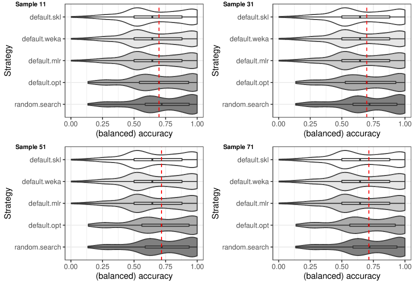
Figure 12: BAC performance distributions obtained by different HP settings evaluated in test datasets with different sample sizes.

(a) CD diagram for sample = 11 and $\alpha=0.05$.

(b) CD diagram for sample = 31 and $\alpha=0.05$.

(c) CD diagram for sample = 51 and $\alpha=0.05$.

(d) CD diagram for sample = 71 and $\alpha=0.05$.

Figure 13: Comparison of the BAC values of the HP setting strategies for SVMs according to the Nemenyi test with $\alpha=0.05$. Groups of strategies that are not significantly different are connected.

Figure 13 shows the Friedman-Nemenyi results, with $\alpha=0.05$, when comparing strategies considering different datasets’ sample sizes separately. The CD diagram at the top show the results for sizes = {11, 31}, while the bottom ones show for sizes = {51, 71}. For all cases, RS was the best-ranked whereas our strategy (default.opt) was the second one, both significantly outperforming the traditional defaults. In addition, it can be observed that our strategy does not present statistically significant differences to the tuning technique when the sample size = {51, 71}, i.e., using the new optimized settings led to equivalent results when compared to RS.

Considering Figure 13, especially the results for the 51 and 71 size samples, we confirm our hypothesis that a small set of new optimized HP settings can improve predictive performance compared to traditional HP default settings. Notably, our strategy is even comparable to a tuning technique, but with a much lower computational cost.

References

- Alcobaça et al. [2020] Alcobaça E, Siqueira F, Rivolli A, Garcia LPF, Oliva JT, de Carvalho ACPLF (2020) Mfe: Towards reproducible meta-feature extraction. Journal of Machine Learning Research 21(111):1–5, URL http://jmlr.org/papers/v21/19-348.html
- Anastacio et al. [2019] Anastacio M, Luo C, Hoos H (2019) Exploitation of default parameter values in automated algorithm configuration. In: Workshop Data Science Meets Optimisation (DSO), Macao, China
- Andradottir [2015] Andradottir S (2015) A review of random search methods. In: Fu MC (ed) Handbook of Simulation Optimization, International Series in Operations Research & Management Science, vol 216, Springer New York, pp 277–292
- Ansótegui et al. [2015] Ansótegui C, Malitsky Y, Samulowitz H, Sellmann M, Tierney K (2015) Model-based genetic algorithms for algorithm configuration. In: Proceedings of the 24th International Conference on Artificial Intelligence, AAAI Press, IJCAI’15, pp 733–739, URL http://dl.acm.org/citation.cfm?id=2832249.2832351
- Bardenet et al. [2013] Bardenet R, Brendel M, Kégl B, Sebag M (2013) Collaborative hyperparameter tuning. In: Dasgupta S, McAllester D (eds) Proceedings of the 30th International Conference on Machine Learning, PMLR, Atlanta, Georgia, USA, Proceedings of Machine Learning Research, vol 28, pp 199–207
- Ben-Hur and Weston [2010] Ben-Hur A, Weston J (2010) A user’s guide to support vector machines. In: Data Mining Techniques for the Life Sciences, Methods in Molecular Biology, vol 609, Humana Press, pp 223–239
- Bergstra and Bengio [2012] Bergstra J, Bengio Y (2012) Random search for hyper-parameter optimization. J Mach Learn Res 13:281–305
- Bergstra et al. [2013] Bergstra J, Yamins D, Cox DD (2013) Making a science of model search: Hyperparameter optimization in hundreds of dimensions for vision architectures. In: Proc. 30th Intern. Conf. on Machine Learning, pp 1–9
- Bergstra et al. [2011] Bergstra JS, Bardenet R, Bengio Y, Kégl B (2011) Algorithms for hyper-parameter optimization. In: Shawe-Taylor J, Zemel RS, Bartlett PL, Pereira F, Weinberger KQ (eds) Advances in Neural Information Processing Systems 24, Curran Associates, Inc., pp 2546–2554
- Birattari et al. [2010] Birattari M, Yuan Z, Balaprakash P, Stützle T (2010) F-Race and Iterated F-Race: An Overview, Springer Berlin Heidelberg, Berlin, Heidelberg, pp 311–336
- Bischl et al. [2016] Bischl B, Lang M, Kotthoff L, Schiffner J, Richter J, Studerus E, Casalicchio G, Jones ZM (2016) mlr: Machine learning in r. Journal of Machine Learning Research 17(170):1–5
- Braga et al. [2013] Braga I, do Carmo LP, Benatti CC, Monard MC (2013) A note on parameter selection for support vector machines. In: Castro F, Gelbukh A, González M (eds) Advances in Soft Computing and Its Applications, Lecture Notes in Computer Science, vol 8266, Springer Berlin Heidelberg, pp 233–244
- Breiman [2001] Breiman L (2001) Random forests. Machine Learning 45(1):5–32, DOI 10.1023/A:1010933404324
- Brochu et al. [2010] Brochu E, Cora VM, de Freitas N (2010) A tutorial on bayesian optimization of expensive cost functions, with application to active user modeling and hierarchical reinforcement learning. CoRR abs/1012.2599
- Brodersen et al. [2010] Brodersen KH, Ong CS, Stephan KE, Buhmann JM (2010) The balanced accuracy and its posterior distribution. In: Proceedings of the 2010 20th International Conference on Pattern Recognition, IEEE Computer Society, pp 3121–3124
- Cawley and Talbot [2010] Cawley GC, Talbot NLC (2010) On over-fitting in model selection and subsequent selection bias in performance evaluation. The Journal of Machine Learning Research 11:2079–2107
- Chang and Lin [2011] Chang CC, Lin CJ (2011) Libsvm: a library for support vector machines. ACM transactions on intelligent systems and technology (TIST) 2(3):27
- Clerc [2012] Clerc M (2012) Standard partcile swarm optimization, 15 pages
- Demšar [2006] Demšar J (2006) Statistical comparisons of classifiers over multiple data sets. The Journal of Machine Learning Research 7:1–30
- Eggensperger et al. [2018] Eggensperger K, Lindauer M, Hoos HH, Hutter F, Leyton-Brown K (2018) Efficient benchmarking of algorithm configurators via model-based surrogates. Machine Learning 107(1):15–41
- Frank et al. [2016] Frank E, Hall MA, Witten IH (2016) The WEKA workbench. Online Appendix for ”Data Mining: Practical Machine Learning Tools and Techniques”, Morgan Kaufmann, Fourth Edition
- Gomes et al. [2012] Gomes TAF, Prudêncio RBC, Soares C, Rossi ALD, nd André C P L F Carvalho (2012) Combining meta-learning and search techniques to select parameters for support vector machines. Neurocomputing 75(1):3–13
- Guo et al. [2008] Guo X, Yang J, Wu C, Wang C, Liang Y (2008) A novel ls-svms hyper-parameter selection based on particle swarm optimization. Neurocomputing 71(16):3211–3215, DOI https://doi.org/10.1016/j.neucom.2008.04.027, advances in Neural Information Processing (ICONIP 2006) / Brazilian Symposium on Neural Networks (SBRN 2006)
- Hauschild and Pelikan [2011] Hauschild M, Pelikan M (2011) An introduction and survey of estimation of distribution algorithms. Swarm and evolutionary computation 1(3):111–128
- Hsu et al. [2007] Hsu CW, Chang CC, Lin CJ (2007) A Practical Guide to Support Vector Classification. Department of Computer Science - National Taiwan University, Taipei, Taiwan
- Hutter et al. [2011] Hutter F, Hoos HH, Leyton-Brown K (2011) Sequential model-based optimization for general algorithm configuration. In: Coello CAC (ed) Learning and Intelligent Optimization, Springer Berlin Heidelberg, Berlin, Heidelberg, pp 507–523
- Hutter et al. [2014] Hutter F, López-Ibáñez M, Fawcett C, Lindauer M, Hoos HH, Leyton-Brown K, Stützle T (2014) Aclib: A benchmark library for algorithm configuration. In: Pardalos PM, Resende MG, Vogiatzis C, Walteros JL (eds) Learning and Intelligent Optimization, Springer International Publishing, Cham, pp 36–40
- Krstajic et al. [2014] Krstajic D, Buturovic LJ, Leahy DE, Thomas S (2014) Cross-validation pitfalls when selecting and assessing regression and classification models. Journal of cheminformatics 6(1):10+
- Lang et al. [2015] Lang M, Kotthaus H, Marwedel P, Weihs C, Rahnenführer J, Bischl B (2015) Automatic model selection for high-dimensional survival analysis. Journal of Statistical Computation and Simulation 85(1):62–76, DOI 10.1080/00949655.2014.929131
- Lemaître et al. [2017] Lemaître G, Nogueira F, Aridas CK (2017) Imbalanced-learn: A python toolbox to tackle the curse of imbalanced datasets in machine learning. Journal of Machine Learning Research 18(17):1–5, URL http://jmlr.org/papers/v18/16-365
- Lemke et al. [2015] Lemke C, Budka M, Gabrys B (2015) Metalearning: a survey of trends and technologies. Artificial intelligence review 44(1):117–130
- Li et al. [2018] Li L, Jamieson K, DeSalvo G, Rostamizadeh A, Talwalkar A (2018) Hyperband: A novel bandit-based approach to hyperparameter optimization. Journal of Machine Learning Research 18(185):1–52, URL http://jmlr.org/papers/v18/16-558.html
- Mantovani [2018] Mantovani RG (2018) use of meta-learning for hyperparameter tuning of classification problems. PhD thesis, Instituto de Ciências Matemáticas e de Computação, Universidade de São Paulo, São Carlos, Brazil
- Mantovani et al. [2015a] Mantovani RG, Rossi ALD, Vanschoren J, Bischl B, de Carvalho ACPLF (2015a) Effectiveness of random search in SVM hyper-parameter tuning. In: 2015 International Joint Conference on Neural Networks, IJCNN 2015, Killarney, Ireland, July 12-17, 2015, IEEE, pp 1–8
- Mantovani et al. [2015b] Mantovani RG, Rossi ALD, Vanschoren J, Carvalho ACPLF (2015b) Meta-learning recommendation of default hyper-parameter values for svms in classification tasks. In: Vanschoren J, Brazdil P, Giraud-Carrier CG, Kotthoff L (eds) Proceedings of the 2015 International Workshop on Meta-Learning and Algorithm Selection co-located with European Conference on Machine Learning and Principles and Practice of Knowledge Discovery in Databases 2015 (ECMLPKDD 2015), Porto, Portugal, September 7th, 2015., CEUR-WS.org, CEUR Workshop Proceedings, vol 1455, pp 80–92
- Mantovani et al. [2019] Mantovani RG, Rossi AL, Alcobaça E, Vanschoren J, de Carvalho AC (2019) A meta-learning recommender system for hyperparameter tuning: predicting when tuning improves svm classifiers. Information Sciences 501:193–221, DOI https://doi.org/10.1016/j.ins.2019.06.005
- Miranda et al. [2014] Miranda P, Silva R, Prudêncio R (2014) Fine-tuning of support vector machine parameters using racing algorithms. In: Proceedings of the 22nd European Symposium on Artificial Neural Networks, Computational Intelligence and Machine Learning, ESANN 2014, pp 325–330
- Padierna et al. [2017] Padierna LC, Carpio M, Rojas A, Puga H, Baltazar R, Fraire H (2017) Hyper-Parameter Tuning for Support Vector Machines by Estimation of Distribution Algorithms, Springer International Publishing, Cham, pp 787–800
- Pedregosa et al. [2011] Pedregosa F, Varoquaux G, Gramfort A, Michel V, Thirion B, Grisel O, Blondel M, Prettenhofer P, Weiss R, Dubourg V, Vanderplas J, Passos A, Cournapeau D, Brucher M, Perrot M, Duchesnay E (2011) Scikit-learn: Machine learning in Python. Journal of Machine Learning Research 12:2825–2830
- Pfisterer et al. [2018] Pfisterer F, van Rijn JN, Probst P, Müller A, Bischl B (2018) Learning multiple defaults for machine learning algorithms. arXiv preprint arXiv:181109409
- Probst et al. [2018] Probst P, Bischl B, Boulesteix AL (2018) Tunability: Importance of hyperparameters of machine learning algorithms. arXiv:1802.09596v3[stat.ML]
- Reif et al. [2012] Reif M, Shafait F, Dengel A (2012) Meta-learning for evolutionary parameter optimization of classifiers. Machine Learning 87:357–380
- Reif et al. [2014] Reif M, Shafait F, Goldstein M, Breuel T, Dengel A (2014) Automatic classifier selection for non-experts. Pattern Analysis and Applications 17(1):83–96
- Ridd and Giraud-Carrier [2014] Ridd P, Giraud-Carrier C (2014) Using metalearning to predict when parameter optimization is likely to improve classification accuracy. In: Vanschoren J, Brazdil P, Soares C, Kotthoff L (eds) Meta-learning and Algorithm Selection Workshop at ECAI 2014, pp 18–23
- van Rijn et al. [2018] van Rijn JN, Pfisterer F, Thomas J, Müller A, Bischl B, Vanschoren J (2018) Meta learning for defaults–symbolic defaults. In: Neural Information Processing Workshop on Meta-Learning
- Santafe et al. [2015] Santafe G, Inza I, Lozano J (2015) Dealing with the evaluation of supervised classification algorithms. Artif Intell Rev 44:467–508
- Shi and Eberhart [1999] Shi Y, Eberhart RC (1999) Empirical study of particle swarm optimization. In: Proceedings of the 1999 Congress on Evolutionary Computation-CEC99 (Cat. No. 99TH8406), IEEE, vol 3, pp 1945–1950
- Simon [2013] Simon D (2013) Evolutionary optimization algorithms. John Wiley & Sons
- Snoek et al. [2012] Snoek J, Larochelle H, Adams RP (2012) Practical bayesian optimization of machine learning algorithms. In: Pereira F, Burges C, Bottou L, Weinberger K (eds) Advances in Neural Information Processing Systems 25, Curran Associates, Inc., pp 2951–2959
- Vanschoren et al. [2014] Vanschoren J, van Rijn JN, Bischl B, Torgo L (2014) Openml: Networked science in machine learning. SIGKDD Explor Newsl 15(2):49–60
- Weerts et al. [2020] Weerts HJP, Mueller AC, Vanschoren J (2020) Importance of tuning hyperparameters of machine learning algorithms. 2007.07588
- Wistuba et al. [2015] Wistuba M, Schilling N, Schmidt-Thieme L (2015) Sequential model-free hyperparameter tuning. In: 2015 IEEE International Conference on Data Mining, pp 1033–1038, DOI 10.1109/ICDM.2015.20