Contiguous Graph Partitioning For Optimal Total Or Bottleneck Communication
Abstract
Graph partitioning schedules parallel calculations like sparse matrix-vector multiply (SpMV). We consider contiguous partitions, where the rows (or columns) of a sparse matrix with nonzeros are split into parts without reordering. We propose the first near-linear time algorithms for several graph partitioning problems in the contiguous regime.
Traditional objectives such as the simple edge cut, hyperedge cut, or hypergraph connectivity minimize the total cost of all parts under a balance constraint. Our total partitioners use space. They run in time, a significant improvement over prior time algorithms due to Kernighan and Grandjean et. al.
Bottleneck partitioning minimizes the maximum cost of any part. We propose a new bottleneck cost which reflects the sum of communication and computation on each part. Our bottleneck partitioners use linear space. The exact algorithm runs in linear time when is for . Our -approximate algorithm runs in linear time when is for , where and are upper and lower bounds on the optimal cost. We also propose a simpler -approximate algorithm which runs in a factor of from linear time.
We empirically demonstrate that our algorithms efficiently produce high-quality contiguous partitions on a test suite of 42 test matrices. When , our hypergraph connectivity partitioner achieved a speedup of (mean ) over prior algorithms. The mean runtime of our bottleneck partitioner was SpMVs.
Index Terms:
Contiguous, Partitioning, Load Balancing, Communication-Avoiding, Chains-On-Chains, Dominance Counting, Least Weight Subsequence, Quadrangle Inequality, Convex, Concave, Monotonic1 Introduction
Sparse matrix multiplication is often the most expensive subroutine in scientific computing applications. When multiplying a dense vector or matrix, we refer to this kernel as SpMV or SpMM respectively. Many applications, such as iterative solvers, multiply by the same sparse matrix repeatedly. Parallelization can increase efficiency, and datasets can be large enough that distributed memory approaches are necessary. A common parallelization strategy is to partition the rows (or similarly, the columns) of the sparse matrix and corresponding elements of the dense vector(s) into disjoint parts, each assigned to a separate processor. While there are a myriad of methods for partitioning the rows of sparse matrices, we focus on the case where the practitioner does not wish to change the ordering of the rows and the parts are therefore contiguous.
There are several reasons to prefer contiguous partitioning. The row ordering may already be carefully optimized for numerical considerations (such as fill-in), the natural row ordering may already be amenable to partitioning, or reordering may simply be too costly to implement on the target architecture. Furthermore, several noncontiguous partitioners (spectral methods or other heuristics [1, 2]) work by producing a one-dimensional embedding of the rows, then using a contiguous partitioner to subsequently “round” the ordering into a partition. Similarly, geometric partitioners partition points by splitting a multidimensional embedding, such as the multidimensional spectral embedding or simply the natural locations of the corresponding mesh cells. The popular multi-jagged geometric approach recursively splits one spatial dimension at a time using a load-balancing contiguous partitioner [3, 4]. As a final example, acyclic partitioning is used to schedule execution of directed acyclic computation graphs. A prominent approach to acyclic partitioning applies contiguous partitioning to a topological ordering of the graph that respects data dependence relationships [5, 6].
Since noncontiguous partitioning to minimize communication costs is NP-Hard [7, 8], one can view contiguous partitioning as a compromise, where the user is asked to use domain knowledge or heuristics to produce a good ordering, but the partitioning can be performed efficiently and optimally. Our algorithms demonstrate that contiguous partitioning can be efficient in theory and practice, and support highly expressive cost models.
We consider two main partitioning objectives, total partitioning and bottleneck partitioning. Traditional partitioning objectives minimize the total communication under the constraint that the work or storage should be approximately balanced. However, in many applications of SpMV or SpMM, such as iterative solvers, all processors wait for the last processor to finish. Therefore, it may be more accurate to minimize the runtime of the longest-running (bottleneck) processor. Here, we model runtime as the combined cost of communication and computation on a part. This allows us to shift work burdens from extroverted processors which communicate frequently to introverted processors which communicate rarely, more efficiently utilizing resources [9].
1.1 Contributions
We propose efficient contiguous partitioners for total and bottleneck objectives. Our algorithms run in linear or near-linear time, representing asymptotic improvements over the state of the art. We evaluate our algorithms experimentally111github.com/peterahrens/ChainPartitioners.jl/tree/2007.16192v4 on a suite of 42 test matrices. We show our algorithms to be efficient in practice. Our partitions are often the quality of computation-balanced partitions or evenly sized partitions on matrices in their natural order, spectral order, or Cuthill-McKee order [10, 11]. Our partitioners are competitive with existing graph partitioning approaches when we account for the runtime of the partitioners themselves.
We address symmetric and nonsymmetric partitions. When the partition is nonsymmetric, we address the cases where either the rows or column partition is considered fixed. Without loss of generality, we consider partitions of the rows of an matrix with nonzeros to run on processors. We normalize our runtimes to the time it takes to perform a sparse matrix-vector multiply (SpMV) on the same matrix.
1.1.1 Contiguous Total Partitioners
The total contiguous partitioning problem includes the traditional simple edge cut, hyperedge cut, and hypergraph connectivity objectives. We propose an exact algorithm for these costs which runs in time
and uses space. This represents a significant improvement (quadratic to near-linear) over the previous time algorithms due to Grandjean et. al. and Kernighan [12, 13]. When and the work was balanced, our total partitioner for hypergraph connectivity runs in an average of SpMVs, a mean speedup of over the existing algorithm.
1.1.2 Contiguous Bottleneck Partitioners
The bottleneck contiguous partitioning problem includes the traditional “Chains-On-Chains” computational load balancing objective. We propose new cost functions which add hypergraph communication terms to the computational load. We propose exact and approximate algorithms for our new costs. Our algorithms use linear space. Our exact algorithm is parameterized by a constant and runs in time
This can be made strictly linear when when is for some constant . Our -approximate algorithm is parameterized by a constant and runs in time
where and are upper and lower bounds on the optimal cost. This can be made strictly linear when is for some constant . Our experiments set to . We also propose a simpler -approximate algorithm that runs in time
which is only near linear but is faster in practice. If the cost functions are monotonic increasing and subadditive, we can derive bounds so that is . When and , our exact, approximate, and lazy bottleneck hypergraph partitioners run in an average of , , and SpMVs over our symmetric test matrices, making our algorithms practical even in situations where the matrix is not heavily reused.
1.1.3 Core Algorithmic Advances
Our algorithms perform structured queries of the cost of various potential parts to determine a good partition. Our results are enabled by three main algorithmic advances.
-
•
We decompose our novel and traditional partitioning objectives into partwise terms, and taxonomize the resulting partwise costs based on the key properties of monotonicity, sub- or super-additivity, and convexity or concavity. We then reduce the task of computing our costs to two dimensional dominance counting (sparse prefix sum) queries. We generalize an offline two-dimensional dominance counting datastructure due to Chazelle to trade construction time for query time, allowing our bottleneck partitioners to run in linear time [14]. Our dominance counting algorithm may also be of interest for two-dimensional rectilinear load balancing problems with linear cost functions [15, 16, 17].
-
•
Our total partitioner reduces the problem to a sequence of constrained convex or concave least-weight-subsequence (LWS) subproblems. We generalize Eppstein’s constrained convex LWS algorithm from part size constraints to arbitrary monotonic constraints [18]. The constrained LWS algorithm (which runs in time ) may be of independent interest for the purposes of partitioning into an arbitrary number of row blocks to minimize total cache misses [19, 20].
-
•
To minimize the bottleneck cost, we adapt state of the art chains-on-chains partitioning algorithms (originally due to Iqbal et. al. and Nicol et. al. [21, 15] and further improved by Pinar et. al. [22]) to support arbitrary monotonic increasing and decreasing cost functions. We simplify the approximate algorithm by relaxing a binary search to a linear search and using an online dominance counter.
2 Background
We index starting from 1. Consider the matrix . We refer to the entry in the row and column of as . A matrix is called sparse if most of its entries are zero. It is more efficient to store sparse matrices in compressed formats that only store the nonzeros. Let be the number of nonzeros in . Without loss of generality, as transposition and format conversion usually run in linear time, we consider the Compressed Sparse Row (CSR) format. CSR stores a sorted vector of nonzero column coordinates in each row, and a corresponding vector of values. This is accomplished with three arrays , , and of length , , and respectively. Locations to of hold the sorted column indices such that , and the corresponding entries of hold the nonzero values.
A -partition of the rows of , assigns each row to a single part . Any partition on elements must satisfy coverage and disjointness constraints.
| (1) |
A partition is contiguous when adjacent elements are assigned to the same part. Formally, is contiguous when,
| (2) |
We can describe a contiguous partition using its split points , where for . Thus, .
We consider graphs and hypergraphs on vertices and edges. Edges can be thought of as connecting sets of vertices. We say that a vertex is incident to edge if . Note that if and only if . Graphs can be thought of as a specialization of hypergraphs where each edge is incident to exactly two vertices. The degree of a vertex is the number of incident edges, and the degree of an edge is the number of incident vertices.
We distinguish between symmetric and nonsymmetric partitioning regimes. A symmetric partitioning regime assumes to be square and that the input and output vectors will use the same partition . Note that we can use symmetric partitioning on square, asymmetric matrices. The nonsymmetric partitioning regime makes no assumption on the size of , and allows the input vector (columns) to be partitioned according to some partition which may differ from the output vector (row) partition . Since our load balancing algorithms are designed to optimize only one partition at a time, we alternate between optimizing or , considering the other partition to be fixed. When is considered fixed and our goal is only to find , we refer to this more restrictive problem as primary alternate partitioning. When is considered fixed and our goal is only to find , we refer to this problem as secondary alternate partitioning. Alternating partitioning has been examined as a subroutine in heuristic solutions to nonsymmetric partitioning regimes, where the heuristic alternates between improving the row partition and the column partition, iteratively converging to a local optimum [23, 24]. Similar alternating approaches have been used for the related two-dimensional rectilinear partitioning regimes [15, 17].
3 Problem Statement
We seek a contiguous partition minimizing either
| (3) |
where is a cost function mapping parts (sets of vertices) to the extended reals (the real numbers and ). We refer to these problems as total or bottleneck partitioning, respectively. The number of parts, , may be fixed or allowed to vary. Because we consider only contiguous parts, we may use as a shorthand for .
The cost function, , might enjoy certain properties which allow us to make algorithmic optimizations. We say that is monotonic increasing if for any ,
| (4) |
and is monotonic decreasing when the inequality is reversed. We say that is superadditive if for any ,
| (5) |
and is subadditive when the inequality is reversed. Finally, we say that is concave when satisfies the quadrangle inequality for any ,
| (6) |
and is convex when the inequality is reversed. Concavity and convexity imply superadditivity and subadditivity, respectively. When the inequality in (5) becomes an equality, we say is additive. Additive functions are subadditive, superadditive, convex, and concave.
Note that negating an increasing, subadditive, or concave cost function will produce a decreasing, superadditive, or convex cost function, respectively. All of our properties are preserved under addition and scaling by positive constants. Subadditivity is preserved under , superadditivity is preserved under . Monotonicity is preserved under both and , but neither concavity nor convexity are preserved under either.
Partitioners often use constraints to reflect storage limits or to balance work. We can use thresholds in our cost functions to reflect such constraints. If our weight limit is , then we define
If is increasing, then is increasing, superadditive, and concave. If is decreasing, then is decreasing, subadditive, and concave. A simple way to add a weight limit on to a cost function would be to form (we assume that times is ). We can also use thresholds to capture discontinuous phenomena like cache effects. For example, one might use thresholds to switch to more expensive cost models when the input or output vectors no longer fit in cache.
3.1 Traditional Partitioning Objectives
Traditional graph and hypergraph partitioning problems map rows of to vertices of a graph or hypergraph, and use edges to represent communication costs. The parts are weighted to represent storage or computation costs, and the objective is to minimize the total communication between a fixed number of parts under an -approximate weight balance constraint like
| (7) |
which we might represent as .
Graph models for symmetric partitioning of symmetric matrices typically use the adjacency representation of a sparse matrix . If , an edge exists between vertices and if and only if . Thus, cut edges (edges whose vertices lie in different parts) require communication of their corresponding columns. However, this model overcounts communication costs in the event that multiple cut edges correspond to the same column, since each column only represents one entry of which needs to be sent. Reductions to bipartite graphs are used to extend this model to the possibly rectangular, nonsymmetric case [24]. Graph partitioning under the “edge cut” seeks to optimize
| (8) |
under balance constraints (7), where . We can rearrange the edge cut (8) objective in the form of Problem (3) by subtracting the constant ,
where is monotonic decreasing and convex.
Inaccuracies in the graph model led to the development of the hypergraph model of communication. Here we use the incidence representation of a hypergraph, . If , edges correspond to columns in the matrix, vertices correspond to rows, and we connect the edge to the vertex when . Thus, if there is some edge which is not cut in a row partition , all incident vertices to must belong to the same part , and we can avoid communicating the input by assigning it to processor in our column partition . In this way, we can construct a secondary column partition such that the number of cut edges in a row partition corresponds exactly to the number of entries of that must be communicated, and the number of times an edge is cut is one more than the number of processors which need to receive that entry of , since one of these processors has that entry of stored locally. By filling in the diagonal of the matrix, this correspondence still holds when the partition is symmetric [8]. To formalize these cost functions on a partition , we define as the set of row parts which contain nonzeros in the column. Tersely, . Hypergraph partitioning with the “hyperedge cut” metric seeks to optimize
| (9) |
and with the “( - 1) cut” metric seeks to optimize
| (10) |
under balance constraints (7), where . Rearranging again by subtracting , we find that minimizing the “hyperedge cut” (9) is equivalent to a partwise objective in the form of Problem (3),
because edges entirely contained within a part are unique to that part. The cost is monotonic decreasing and convex. If we instead add to the “( - 1) cut” (10), we obtain
where the last equality comes from counting incidences over parts rather than over edges. The cost is monotonic increasing and convex.
If we block the rows of a matrix on a serial processor for caching purposes, also corresponds to the number of cache misses on when the row block’s portion of fits in cache. While hypergraph partitioning is usually applied to distributed settings with a fixed number of processors and a balance constraint on nonzeros, this setting would allow variable and limit the number of rows in each part (since each row corresponds to a cached entry of .) [19, 20]
The hypergraph model better captures communication in our kernel, but heuristics for noncontiguous hypergraph partitioning problems can be expensive. For example, state-of-the-art multilevel hypergraph partitioners recursively merge pairs of similar vertices at each level. Finding similar pairs usually takes quadratic time [8, 25].
Both the graph and hypergraph formulations minimize total communication subject to a work or storage balance constraint, but it has been observed that the runtime depends more on the processor with the most work and communication, rather than the sum of all communication [24, 26]. Several approaches seek to use a two-phase approach to nonsymmetric partitioning where the matrix is first partitioned to minimize total communication volume, then the partition is refined to balance the communication volume (and other metrics) across processors [27, 28, 29]. Other approaches modify traditional hypergraph partitioning techniques to incorporate communication balance (and other metrics) in a single phase of partitioning [30, 31, 32]. Given a row partition, Bisseling et. al. consider column partitioning to balance communication (the secondary alternate partitioning regime) [33].
While noncontiguous primary and secondary graph and hypergraph partitioning are usually NP-Hard [34, 35, 33], the contiguous case is much more forgiving. Kernighan proposed a dynamic programming algorithm which solves the contiguous graph partitioning problem to optimality in quadratic time, and this result was extended to hypergraph partitioning by Grandjean and Uçar [13, 36].
Simplifications to the cost function lead to faster algorithms. If we ignore communication and minimize only the maximum amount of work in a noncontiguous partition (where the cost of a part is modeled as the sum of some per-row cost model), our partitioning problem becomes equivalent to bin-packing, which is approximable using straightforward heuristics that can be made to run in log-linear time [37]. The “Chains-On-Chains” partitioning problem also optimizes a linear model of work, but further constrains the partition to be contiguous. Chains-On-Chains has a rich history of study, we refer to [22] for a summary. These problems are often described as “load balancing” rather than “partitioning.” In Chains-On-Chains partitioning, the work of a part is typically modeled as directly proportional to the number of nonzeros in that part. Formally, Chains-On-Chains seeks the best contiguous partition under
| (11) |
where . This objective is already in the form of Problem 3, and the cost model is monotonic increasing and additive.
This cost model is easily computable, and algorithms for Chains-On-Chains partitioning can run in sublinear time. Nicol observed that the work terms for the rows in Chains-On-Chains partitioners can each be augmented by a constant to reflect the cost of vector operations in iterative linear solvers [38]. Local refinements to contiguous partitions have been proposed to take communication factors into account, but our work proposes the first globally optimal linear-time contiguous partitioner with a communication-aware cost model [39, 2].
3.2 Novel Objectives
As we will soon see, the techniques used to solve Chains-On-Chains problems can be applied to any monotonic bottleneck objectives in contiguous settings. [22, 40, 41]. In fact, since the runtime of parallel programs depends on the longest-running processor, bottleneck partitioning may be more accurate than total partitioning in parallel settings. Therefore, we propose several monotonic cost models for use in bottleneck partitioning.
Most applications of SpMV or SpMM don’t have a synchronization point between communication and computation, so we model the runtime of each processor as the sum of work and communication. The inner loop of the conjugate gradient method, for example, has two synchronization points where all processors wait for the results of a global reduction (a dot product) [42, Chapter 6]. This separates the inner loop into two phases; the dominant phase contains our SpMV or SpMM. The processors first send and receive the required elements of their local portions of the input vector , then multiply by to produce . This phase also contains some elementwise vector operations. We model the per-row computation cost (due to dot products, vector scaling, and vector addition) with the scalar , and the per-entry computation costs (due to matrix multiplication) with the scalar . Thus, the computational work on a processor can be described as
| (12) |
which is monotonically increasing in .
In distributed memory settings, both the sending and the receiving node must participate in transmission of the message. We assume that the runtime of a part is proportional to the sum of local work and the number of received entries. This differs from the model of communication used by Bisseling Et. Al., where communication is modeled as proportional to the maximum number of sent entries or the maximum number of received entries, whichever is larger [33]. While ignoring sent entries may seem to represent a loss in accuracy, there are several reasons to prefer such a model. Processors have multiple threads which can perform local work or process sends or receives independently. If we assume that the network is not congested (that sending processors can handle requests when receiving processors make them), then the critical path for a single processor to finish its work consists only of receiving the necessary input entries and computing its portion of the matrix product. We model the cost of receiving an entry with the scalar .
3.2.1 Nonsymmetric Bottleneck Cost Modeling
Since it admits a more accurate cost model, we consider the nonsymmetric partitioning regime first. This regime considers only one of the row (output) space partition or the column (input) space partition , considering the other to be fixed.
We model our matrix as an incidence hypergraph. The nonlocal entries of the input vector which processor must receive are the edges incident to vertices such that . We can express this tersely as . Thus, our cost model for the alternating regime is
| (13) |
which is monotonically increasing in and decreasing in . Intuitively, adding rows to the processor increases work and communication, while adding columns decreases communication.
While we require the opposite partition to be fixed, we will only require the partition we are currently constructing to be contiguous. Requiring both and to be contiguous is sometimes but not always desirable; such a constraint would limit us to matrices whose nonzeros are clustered near the diagonal. Allowing arbitrary fixed partitions gives us the flexibility to use other approaches for the secondary alternate partitioning problem. For example, one might assign each column to an arbitrary incident part to optimize total communication volume as suggested by Çatalyurek [8]. We also consider the similar greedy strategy to assign each column to a currently most expensive incident part, attempting to reduce the cost of the most expensive part.
Of course, since our alternating partitioning regime assumes we have a fixed or , we need an initial partition. We propose starting by constructing because this partition involves more expensive tradeoffs between work and communication. Since we would have no to start with, we assume no locality, upper-bounding the cost of communication and removing from our cost model. In the hypergraph model, processor receives at most entries of the input vector. Thus, our cost model would be
| (14) |
which is monotonically increasing in .
Note that any column partition will achieve or improve on the modeled cost (14).
3.2.2 Symmetric Bottleneck Cost Modeling
The symmetric case asks us to produce a single partition which will be used to partition both the row and column space simultaneously. We do not need to alternate between rows and columns; by adjusting scalar coefficients, we can achieve an approximation of the accuracy of the nonsymmetric model by optimizing a single contiguous partition under objective (3). Replacing with in cost (13) yields,
| (15) |
Unfortunately, the factor is not monotonic. However, notice that is monotonic. Assume that each row of the matrix has at least nonzeros (in linear solvers, should be at least two, or less occupied rows could be trivially computed from other rows.) We rewrite cost (15) in the following form,
| (16) |
This function is monotonic when the coefficients on all terms are positive. We therefore require
| (17) |
Informally, constraint (17) asks that the rows and dot products hold “enough” local work to rival communication costs. These conditions roughly correspond to situations where it is cheaper to communicate an entry of than it is to compute it if the relevant entries of were stored locally. These constraints are most suitable to matrices with heavy rows, because increasing the number of nonzeros in a row increases the amount of local work and the communication footprint, but not the cost to communicate the single entry of output corresponding to that row.
Depending on the sparsity of our matrix, we may approximate the modeled cost of the matrix by assuming to be larger than it really is. If there are at most “underfull” rows with less than nonzeros, then cost (15) will be additively inaccurate by at most .
4 Computing Costs
Our contiguous partitioners will probe the cost of many potential parts, and rely on datastructures that efficiently answer such queries. Our goal is to create datastructures to compute costs (8), (9), (10), (11), (13), (14), and (16).
In (13), we compute as . In (16), since is just with the diagonal of the matrix filled in, we only consider the latter term. One can fill the diagonal explicitly, or compute the result lazily to avoid a copy of the matrix.
Therefore, apart from constants, we need only compute the unique terms , , , , , and .
Our algorithms only make contiguous queries of the form or , although the fixed partition or may not be contiguous, respectively.
Our first term, , is easy to compute in constant time. Similarly, since the vector in CSR format is a prefix sum (cumulative sum) of the number of nonzeros in each row , we can compute in constant time. If our matrix is not stored in CSR format, we can usually construct in linear time.
The only term with an explicit dependence on is . When is fixed, we can construct sorted list representations of each set in linear time and space (using, for example, a histogram sort and deleting adjacent duplicates). This allows us to evaluate in time by searching our list for the boundaries of the contiguous region of elements which are also in .
What remains to be shown is how to compute the remaining terms for various contiguous when is held constant.
4.1 Reduction to Dominance Counting
In this section, we reduce computing our remaining terms to two-dimensional dominance counting, a classic computational geometry problem. Consider points of the form in an integer grid . We say that a point dominates a point if and . The dominance counting problem in two dimensions asks for a data structure to count the number of points dominated by each query point. Note that by negating either the first or second coordinate, we can reverse the first or second inequality to ask for containment constraints.
We start with the term , which counts the number of nonzero entries where . When we represent it with the point , otherwise we represent it with the point . Since , the number of points dominated by is the number of nonzeros where both coordinates are contained in .
We handle the term similarly. In linear time, we compute , the smallest and largest elements of each . This corresponds to the position of the first and last nonzero in each column of . Since , the number of points dominated by is the number of columns whose nonzeros are completely contained by , or .
The final two terms, and , present more of a challenge. These quantities concern the size of the set of distinct nonzero column locations in some row part. We know that is an easy upper bound on , but it overcounts columns for each row they are incident to. If we were somehow able to count only the first appearance of a nonzero column in our part, we could compute . We refer to the pair of a nonzero entry and the next (redundant) nonzero entry in the column as a link. If the nonzero occurs at row in some column and the closest following nonzero occurs at in that column, we call this a link, and represent it with the point . Thus,
| (18) |
We have already shown how to compute the first term from the array. The second term is the number of points dominated by . Figure 2 illustrates this relationship. Our reduction is almost equivalent to the reduction from multicolored one-dimensional dominance counting to two-dimensional standard dominance counting described by Gupta et. al., but our reduction requires only one dominance query, while Gupta’s requires two [43]. We have re-used the values in the array of the link matrix in CSR format to avoid the second dominance query (dominance queries can be expensive in practice).
Finally, to compute when is fixed, we can logically split into separate matrices where is where all columns other than are zeroed out. Note that the total number of nonzeros is still . Computing on gives us .
To avoid separate dominance counting problems for each column part , we concatenate the separate problems into one problem and then transform our problem into rank space [44, 14]. Recall that our points are given to us in -major, -minor order. We transform to rank space by resorting the points into a -major, -minor order . Our transformation maps a point to its position pair . Notably, if and only if and if and only if , so our dominance counts are preserved under our transformation. If we store our two orderings, we can use binary search to find the transformed point at query time.
We can sort the links first by their column part, then into -major and -major orders in linear time with, for example, two histogram sorts. By storing the boundaries of where each part’s subproblem begins and ends, we can then resolve dominance queries within the region corresponding to the target part.
4.2 Online Dominance Counting
First, we consider a simple direct method for incremental dominance counting, adapted from [45], the most directly applicable method of its kind [36, 39, 2, 46]. The datastructure requires words, can be constructed in time, and given we have just answered a query for , we can answer a query for in time, and a query for or in constant time.
Our datastructure starts at with a counter of dominated points and a vector initialized to . To increment , we iterate over each point with right coordinate , incrementing by one each time, and incrementing when . To decrement , we simply add to . To set to , we need only set to .
When links are needed, we can use a vector of size to record the last time we have seen a particular nonzero column as advances from the top of the matrix to the bottom. The next time we see a nonzero in the same column, we can report the corresponding link.
When we compute for various , we maintain separate counters for the range for each column part, so that we may increment in constant time.
The online approach is efficient in settings when we wish to compute the cost of parts for many starting points corresponding to a fixed end point, or for many end points corresponding to a fixed start point. It is also a simple way to compute the cost of a single partition once.
4.3 Offline Dominance Counting
Offline dominance counting is more appropriate when our partitioner makes fewer queries of more arbitrary intervals. The two dimensional problem has been the subject of intensive theoretical study [14, 47, 48]. However, because of the focus on only query time and storage, little attention has been given to construction time, which is always superlinear. Therefore, we modify Chazelle’s algorithm to allow us to trade construction time for query time [14].
Dominance counting (and the related semigroup range sum problem [49, 50, 47]) are roughly equivalent to the problem of computing prefix sums on sparse matrices and tensors in the database community. These data structures are called “Summed Area Tables” or “Data Cubes,” and they value dynamic update support and low or constant query time at the expense of storage and construction time. We refer curious readers to [51] for an overview of existing approaches, with the caution that most of these works reference the size of a naive dense representation of the summed area table when they use words like “sublinear” and “superlinear.”
Chazelle’s dominance counting algorithm uses linear space in the number of points to be stored, requiring log-linear construction time and logarithmic query time. We adapt this structure to a small integer grid, allowing us to trade off construction time and query time. Whereas Chazelle’s algorithm can be seen as searching through the wake of a merge sort, our algorithm can be seen as searching through the wake of a radix sort. Our algorithm can also be thought of as a decorated transposition of a CSR matrix. Because the algorithm is so detail-oriented, we give a high-level description, but leave the specifics to the pseudocode presented in Algorithms 1 and 2.
Algorithm 1.
Construct the dominance counting data structure over points , ordered on initially. We assume we are given the coordinates in a vector . We require that .
Algorithm 2.
Query the dominance counting data structure for the number of points dominated by .
In this section, assume we have been given points in the range . Since these points come from CSR matrices or our link construction, we assume that our points are initially sorted on their coordinates () and we have access to an array to describe where the points corresponding to each value of starts. If this is not the case, either the matrix or the following algorithm can be transposed, or the points can be sorted with a histogram sort in time.
The construction phase of our algorithm successively sorts the points on their coordinates in rounds, starting at the most significant digit and moving to the least. We refer to the ordering at round as . We use rounds, each with bit digits, where is the smallest integer such that . Let refer to the most significant group of bits (the digit). Formally,
At each round , our points will be sorted by the top bits of their coordinates using a histogram sort in each bucket formed by the previous round. We use an array (similar to ) to store the starting position of each bucket in the current ordering of points. Formally, will record the starting position for points where . Note that is of size instead of , as one might expect, to allow as a possible value for during query time.
Although we can interpret the algorithm as resorting the points several times, each construction phase only needs access to its corresponding bit range of coordinates (the keys) in the current ordering. The query phase needs access to the ordering of keys before executing each phase. Thus, the algorithm iteratively constructs a vector , where the group of bits in corresponds to the group of bits in current ordering of coordinates (). As the construction algorithm proceeds, we can use the lower bits of to store the remaining coordinate bits to be sorted.
Each phase of our algorithm needs to sort buckets. Our histogram sort uses a scratch array of size to sort a bucket of points in time. Thus, we can sort the buckets of level in time, and bucket sorting takes time in total over all levels.
A query requests the number of points in our data structure dominated by . In the initial ordering, is equivalent to . Thus, the dominating points reside within the first positions of the initial ordering. Our algorithm starts by counting the number of points such that and . All remaining dominating points satisfy , so let be the number of points and . After our first sorting round, the set of points in the initial ordering where would have been stored contiguously, and therefore the first of them satisfy . We can then apply our procedure recursively within this bucket to count the number of dominating points.
We have left out an important aspect of our algorithm. Our query procedure needs to count the number of dominating points that satisfy within ranges of that agree on the top bits of each . While stores the requisite ranges of , we still need to count the points. In time, for a particular value of , we can walk from left to right, using a scratch vector of size to count the number of points we see with each value of . If we cache a prefix sum of our scratch vector once every points (the prefix sum takes time), we can use the cache to jump-start the counting process at query time. During a query, after checking our cached count in constant time, we only need to count a maximum of points at each level to obtain the correct count. Our cache is a 3-tensor , where stores the number of points such that and . If we cache every points, computing takes time per phase. The vector uses words, the vector uses words, the vector uses words, and the tensor uses at most words. The runtime and storage of our offline algorithms are summarized in Table I.
We consider two ways to set , , and . Chazelle proposed setting , , and . When , each key is one bit, and Chazelle suggested we “transpose” the array by storing a bit-packed vector for each level. Because the size of a word bounds the size of the input, we can count the bits at each level of the query step with a constant number of bit-counting instructions, saving a factor of at query time. While storage would be linear and query time would be logarithmic, constructing a dominance counter with these settings would require passes. In rank space, this would require an onerous passes for just nonzeros.
We also consider setting , the height of the tree and the number of passes, to a small constant like or , while keeping storage costs linear, since storage is often a critical resource in scientific computing. For correctness, we minimize subject to . We minimize subject to to ensure that the footprint of our dominance counter is at most four times the size of . These settings do not permit the bit-counting optimization at query time because the digits become larger than a single bit.
When our points come from a rank space transformation, then and become . Note that transforming to rank space simplifies our algorithm because and become the identity and we no longer need to store them. However, we do need to store our orderings of and values, so the storage requirement is the same and . Although we need to perform binary search for rank-space queries, the runtime is dominated by the query time in both parameterizations that we consider.
| Settings | Generic | constant | |
| Construct | |||
| Query | |||
| Storage |
5 Bottleneck Partitioners
Pinar et. al. present a multitude of algorithms for optimizing linear cost functions [22]. We examine both an approximate and an optimal algorithm, and point out that with fairly minor modifications they can be modified to optimize arbitrary monotonic increasing or decreasing cost functions, given an oracle to compute the cost of a part. We chose the approximate “-BISECT+” algorithm (originally due to Iqbal et. al. [21]) and the exact “NICOL+” algorithm (originally due to Nicol et. al. [15]) because they are easy to understand and enjoy strong guarantees, but use dynamic split point bounds and other optimizations based on problem structure, resulting in empirically reduced calls to the cost function.
Since the approximate algorithm introduces many key ideas which are expanded upon in the exact algorithm, we start with our adaptation of the “-BISECT+” partitioner, which produces a -partition within of the optimal cost when it lies within the given bounds.
If our cost is monotonic increasing, the optimal partition of a contiguous subset of rows cannot cost more than the optimal partition of the whole matrix, since we could simply truncate a partition of the entire set of rows to the subset in question and achieve the same or lesser cost. Therefore, if we know that there exists a -partition of cost , and we can set the endpoint of the first part to the largest such that , there must exist -partition of the remaining columns that starts at and costs at most . This observation implies a procedure that determines whether a partition of cost is feasible by attempting to construct the partition, maximizing split points at each part in turn. This procedure is called a Probe. Clearly, using linear search for split points, Probe only uses evaluations of the cost function. If Probe uses binary search for split points, it only needs evaluations of the cost function. We can repeatedly call Probe to search the space of possible costs, stopping when our lower bound on the cost is within of the upper bound. Note that if we had the optimal value of a -partition, a single call to Probe can recover the split points. While Pinar et. al. use this fact to simplify their algorithms and return only the optimal partition value, our cost function is more expensive to evaluate than theirs, so our algorithms have been modified to compute the split points themselves without increasing the number of evaluations of the cost function [22].
The intuition in the monotonic decreasing case is the opposite of the monotonic increasing case. Instead of searching for the last split point less than a candidate cost, we search for the first. Instead of looking for a candidate partition which can reach the last row without exceeding the candidate cost, we look for a candidate partition which does not need to exceed the last row to achieve the candidate cost. The majority of changes reside in the small details, which we leave to the pseudocode.
Our adapted bisection algorithm is detailed in Algorithm 4. Algorithm 4 differs from the algorithm presented by Pinar et. al. in that it allows for decreasing functions, is stated in terms of possibly different for each part, does not assume to be zero, allows for an early exit to the probe function, returns the partition itself instead of the best cost (this avoids extra probes needed to construct the partition from the best cost), and constructs the dynamic split index bounds in the algorithm itself, instead of using more complicated heuristics (which may not apply to all cost functions) to initialize the split index bounds. Note that we assume only for the purposes of providing a relative approximation guarantee.
Algorithm 4 considers at most candidate partition costs. If we use a linear search and online (rank space) dominance counters, Probe runs in linear time and Algorithm 4 runs in time
| (19) |
If we use binary search and offline (rank space) dominance counters with constant , Algorithm 4 runs in time
| (20) |
While the binary-searching algorithm has a better asymptotic runtime, the linear-search algorithm can take advantage of the simpler linear dominance counters, and may perform better on smaller problems when is high and therefore the number of probes is low.
The key insight made by Nicol et. al. which allows us to improve our bisection algorithm into an exact algorithm was that there are only possible costs which could be a bottleneck in our partition, corresponding to possible pairs of split points that might define a part [15]. Thus, Nicol’s algorithm searches the split points instead of searching the costs, and achieves a strongly polynomial runtime. We will reiterate the main idea of the algorithm, but refer the reader to [22] for more detailed analysis.
Assume that we know the starting split point of processor to be . Consider the ending point in a partition of minimal cost. If were a bottleneck (longest running processor) in such a partition, then would be the overall cost of the partition, and we could use this cost to bound that of all other processors. If were not a bottleneck, then should be strictly less than the minimum feasible cost of a partition, and it would be impossible to construct a partition of cost . Thus, Nicol’s algorithm searches for the first bottleneck processor, examining each processor in turn. When we find a processor where the cost is feasible, and less than the best feasible cost seen so far, we record the resulting partition in the event this was the first bottleneck processor. Then, we set so that is the greatest infeasible cost and continue searching, assuming that processor was not a bottleneck.
We have made similar modifications in our adaptation of “NICOL+” as we did for our adaptation of “-BISECT+.” Primarily, the algorithm now handles monotonic decreasing functions. We also phrase our algorithm in terms of potentially multiple , construct our dynamic split point bounds inside the algorithm instead of using additional heuristics, make no assumptions on the value of , allow for early exits to the probe function, and return a partition instead of an optimal cost. We also consider bounds on the cost of a partition to be optional in this algorithm. Our adaptation of “NICOL+” ([22]) for general monotonic part costs is presented in Algorithm 5.
Although “NICOL+” uses outcomes from previous searches to bound the split points in future searches, a simple worst-case analysis of the algorithm shows that the number of calls to the cost function is bounded by
| (21) |
Using offline (rank space) dominance counters with constant , Algorithm 4 runs in time
| (22) |
We say that grows polynomially slower than when is for some constant . Thus, the approximate partitioner runs in linear time if grows polynomially slower than . If costs are subadditive, then we only need , and therefore , to grow polynomially slower than . The exact partitioner runs in linear time if grows polynomially slower than . Our algorithms can run in linear time precisely when our partitioners use polynomially sublinear queries, since we are able to offset polynomial query time decreases with logarithmic construction time increases.
For our practical choice of , needs to grow polynomially slower than for linear time approximate partitioning and needs to grow polynomially slower than for linear time exact partitioning. However, both algorithms use dynamic bounds on split indices to reduce the number of probes, so they are likely to outperform these worst-case estimates. Furthermore, , the number of processors, is often a relatively small constant.
Algorithm 3.
Given a monotonic increasing (or decreasing) cost function defined on pairs of split points, a starting split point , and a maximum cost , find the greatest (least, respectively) such that , , and . Returns (returns , respectively) if no cost at most can be found. Changes needed for decreasing functions are marked with .
Algorithm 4 (BISECT Partitioner).
Given monotonic increasing cost function(s) defined on pairs of split points, find a contiguous -partition which minimizes
to a relative accuracy of within the range , if such a partition exists. This is an adaptation of the “-BISECT+” algorithm by Pinar et. al. [22], which was a heuristic improvement on the algorithm proposed by Iqbal et. al. [21]. We assume that Probe shares scope with bisectpartition. Changes needed for the case where all are monotonic decreasing are marked with .
Algorithm 5 (NICOL Partitioner).
Given monotonic increasing cost function(s) defined on pairs of split points, find a contiguous -partition which minimizes
within the range , if such a partition exists. This is an adaptation of the “NICOL+” algorithm by Pinar et. al. [22], which was a heuristic improvement on the algorithm proposed by Nicol et. al. [15]. We assume that ProbeFrom shares scope with NicolPartition. Changes needed for the case where all are monotonic decreasing are marked with .
5.1 Bounding the Costs
Algorithm 4, our approximate bottleneck partitioner, requires upper and lower bounds on the cost function, and both Algorithm 4 and 5 should perform better when given better initial bounds.
Given a monotonic increasing cost function over a set of vertices , and are naive lower and upper bounds on the bottleneck cost of a -partition. These become upper and lower bounds when is decreasing, respectively.
However, we can use subadditivity in increasing cost functions to increase the lower bound on the bottleneck cost of a -partition. Using subadditivity, , and therefore,
| (23) |
Finding good lower bounds on partition costs can be difficult. Costs like (14) and (15) are subadditive and use the same cost for each part, so they obey (23). However, other costs such as (13) use different functions on each part, and therefore we cannot apply equation (23).
We can work around this limitation by lower-bounding all the functions by the same subadditive one, then applying equation (23). For example, one might lower bound only the work terms in the cost function, since these are uniform across partitions. As another example, one might assume that all threshold functions are zero when calculating a lower bound.
Subadditivity does not help us bound monotonic decreasing cost functions. For these costs, it may make sense to simply use and as upper and lower bounds on the cost.
6 Total Partitioners
Total partitioning under Problem (3) is quite similar to the least weight subsequence problem, which we phrase as evaluating the dynamic program
| (24) |
for when is readily computable from . When there is no constraint on the number of parts, we can minimize the sum (3) by setting , and following the back pointers to construct . If, however, we wish to constrain the number of parts to be , then we must apply Problem (24) times, producing separate cost and pointer vectors and , where in the application of (24), . The naive dynamic programming algorithm for variable makes queries to the cost function, and runs in time using our online dominance counters in rank space (we assume the inner loop over is evaluated in reverse). The naive dynamic programming algorithm for fixed makes queries and runs in time using our online dominance counters in rank space. If the cost function is uniform across parts, we can reduce this to by evaluating once for each interval and using that value to update simultaneous LWS recurrences. We refer to this as the “simultaneous” dynamic programming approach.
Previous approaches point out that when the weight of each part is monotonic and constrained, we can use lower and upper bounds on split points in our dynamic program to obtain heuristic improvements [36, 45]. First, when evaluating the recurrence of (24), if we evaluate starting at and work backwards towards , the weight of the candidate part will only increase, and we can stop the recurrence as soon as the weight limit is exceeded. Note also that if , the first feasible will be greater than the first feasible .
Additionally, when is fixed, we can bound the range of feasible by considering the least and greatest might be given that the previous parts and following parts are weight constrained. If are the bounds on the split points for the partition, then we can define as the least index satisfying , and as the greatest index satisfying . We can compute these split point bounds in linear time using online dominance counters and simply walking the matrix once from top to bottom and once from bottom to top. If the weight is simply a limit on the number of rows in each part, these heuristic improvements would bring the running time down to and , respectively. The “simultaneous” version would run in time .
Unfortunately, these techniques still require roughly quadratic time in general. We now show how the techniques described in this paper can bring the runtime down to log-linear time using convexity or concavity in the cost function.
Efficient algorithms exist to solve (24) when is concave or convex [52, 53, 54]. In this work, we focus on linearithmic solutions because they are simple to implement and work well in practice. The solutions of Galil and Giancarlo can solve (24) for convex or concave cost functions in steps, using only one query to the cost function in each step. Unfortunately, these queries are unstructured, so we muse use offline dominance counters. Using Chazelle’s parameterization in rank space where in Table I, the runtime of the resulting least weight subsequence algorithm becomes , and when is fixed, the runtime becomes .
However, while concave cost functions are still concave after adding monotonic balance constraints, convex functions are no longer convex after adding such constraints. Since most of our atoms are convex, we must modify our least weight subsequence algorithm to handle such cases. We take a similar approach to Eppstein, who formulated an algorithm for cost functions which are alternately convex, then concave, then convex, et cetera [18]. While the alternations considered by Eppstein were constrained to fixed width intervals, we consider only the case where we have a convex cost subject to an upper limit on a monotonic weight function. The width of the feasible region may therefore be irregular. While we will not consider an arbitrary number of alternations in the cost, our transition from a convex cost to the concave constraint is more general than the fixed-width intervals considered by Eppstein.
Let be the least index such that . Notice that if , . Consider the sequence of at most split points such that . We can construct in reverse starting at and following the pointers . Our algorithm to compute (24) works in batches corresponding to each range .
Given , consider the problem of computing
for . We split the feasible range of the indices into two subproblems, a more complicated setup phase,
and a simpler cleanup phase,
The cleanup phase can be computed with any standard algorithm for (24), but we need to transform the setup phase first before reducing to (24). If , let be defined as
Since , every element of is less than every element of . When , the interval is feasible. Finally, if and is feasible, there exists where . Thus, we can compute the setup phase with the transformed least weight subsequence problem
and finally setting , where is the greatest index such that . We pick the greatest such index so that the full feasible range of is included.
Each least weight subsequence subproblem can be computed with Galil and Giancarlo’s algorithm using steps, where is the length of the problem. Thus, the setup phase of each segment of length can be computed in steps and the cleanup phase takes steps. Since and there are at most segments, the overall algorithm again runs in steps. Each step involves a constant number of calls to the cost function. While linearithmic LWS algorithms obviate the need for feasible range optimizations within each LWS subproblem, we can still use the feasible range to restrict the size of each LWS subproblem in our -step solution to the fixed- partitioning problem.
7 Results
We compare our partitioners on a set of 42 sparse matrices. We include matrices used by Pinar and Aykanat to evaluate solutions to the Chains-On-Chains problem [22] (minimizing the maximum work without reordering), matrices used by Çatalyurek and Aykanat to evaluate multilevel hypergraph partitioners (minimizing the sum of communication) [8], and matrices used by Grandjean and Uçar to evaluate contiguous hypergraph partitioners (minimizing the sum of communication without reordering) [36]. Since we intend to partition without reordering, we also chose some additional matrices of our own to introduce more variety in the tested sparsity patterns. We exclude “Qaplib/lp_nug30” as KaHyPar could not partition it in under 24 hours. The test suite is summarized in Table II.
Symmetric Matrices
| Group / Matrix | ||
| Boeing/ ct20stif | KK | M |
| Boeing/ pwtk | KK | M |
| Chen/ pkustk03 | KK | M |
| Chen/ pkustk14 | KK | M |
| Cunningham/ qa8fk | KK | M |
| Gupta/ gupta2 | KK | M |
| HB/ bcsstk30 | KK | M |
| HB/ bcsstk32 | KK | M |
| HB/ dwt_607 | K | |
| HB/ sherman3 | KK | K |
| Hamm/ bcircuit | KK | K |
| Mulvey/ finan512 | KK | K |
| Nasa/ nasasrb | KK | M |
| PARSEC/ H2O | KK | M |
| Rothberg/ cfd1 | KK | M |
| Schenk_IBMNA/ c-64 | KK | K |
| Simon/ venkat01 | KK | M |
| TKK/ smt | KK | M |
Asymmetric Matrices Group / Matrix ATandT/ onetone1 KK K ATandT/ onetone2 KK K Averous/ epb3 KK K Bomhof/ circuit_4 KK K Grund/ bayer01 KK K HB/ gemat11 KK K Hollinger/ g7jac180 KK K Hollinger/ mark3jac140sc KK K LPnetlib/ lp_cre_b KK K LPnetlib/ lp_cre_d KK K LPnetlib/ lp_ken_11 KK K LPnetlib/ lp_ken_13 KK K LPnetlib/ lpi_gosh KK K Mallya/ lhr07 KK K Mallya/ lhr14 KK K Mallya/ lhr17 KK K Mallya/ lhr34 KK K Mallya/ lhr71c KK M Meszaros/ co9 KK K Meszaros/ cq9 KK K Meszaros/ mod2 KK K Meszaros/ nl KK K Meszaros/ world KK K Shyy/ shyy161 KK K
In addition to partitioning natural orderings, we also evaluate our algorithms on two of the most popular bandwidth-reducing algorithms, the Reverse Cuthill-McKee (RCM) [10] and spectral [11] orderings, which have a history of application to partitioning [23, 55]. The RCM ordering uses a breadth-first traversal of the graph, prioritizing lower degree vertices first. We follow the linear-time implementation described in [56]. The spectral reordering orders vertices by their values in the Fiedler vector, or the second-smallest eigenvector of the Laplacian matrix. We used the default eigensolver given in the Laplacians.jl library (github.com/danspielman/Laplacians.jl), the only eigensolver we tested that was able to solve all our largest, worst-conditioned problems in a reasonable time. In order to apply these reorderings to asymmetric matrices, we instead reorder a bipartite graph where nodes correspond to rows and columns in our original matrix, which are connected by edges when nonzeros lie at the intersection of a row and a column, as described by Berry et. al. [57].
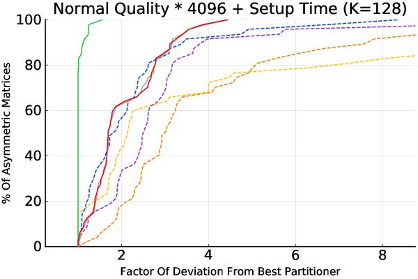
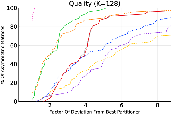
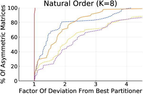
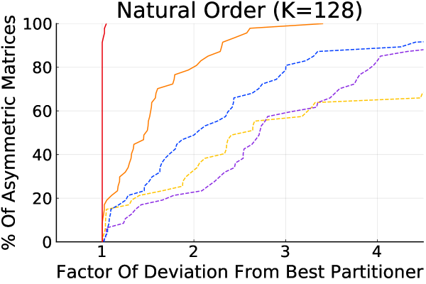
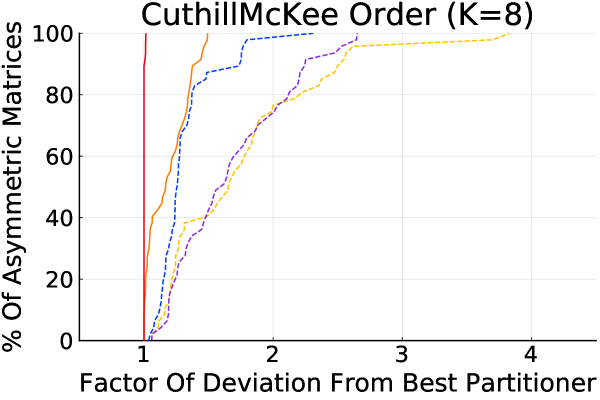
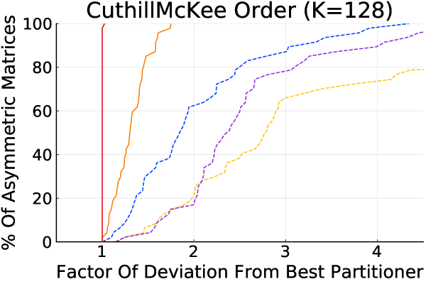
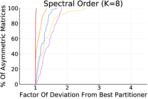
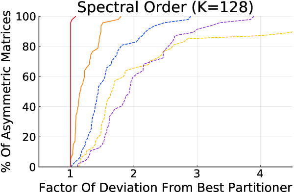
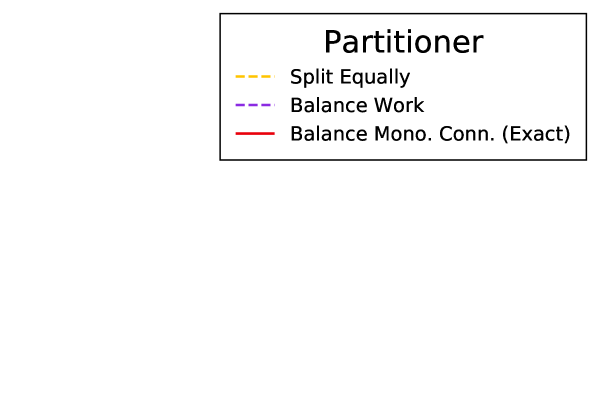
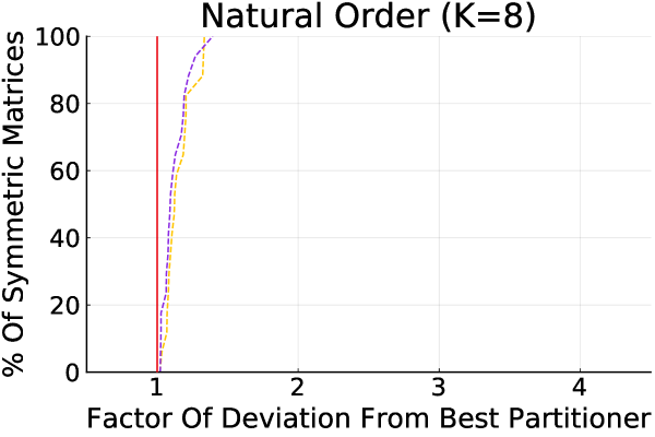
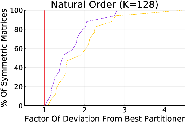
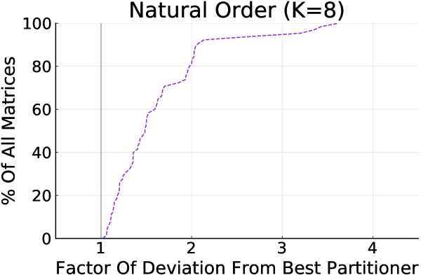
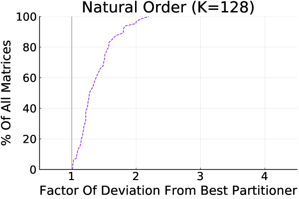
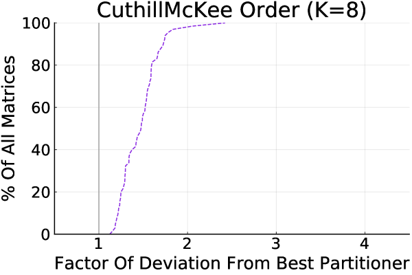
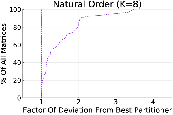
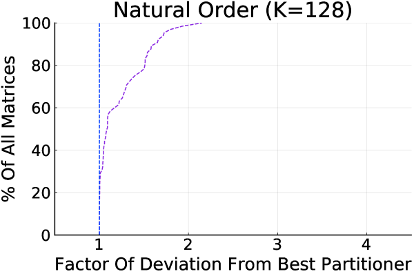
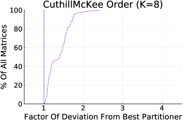
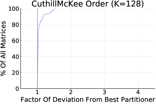
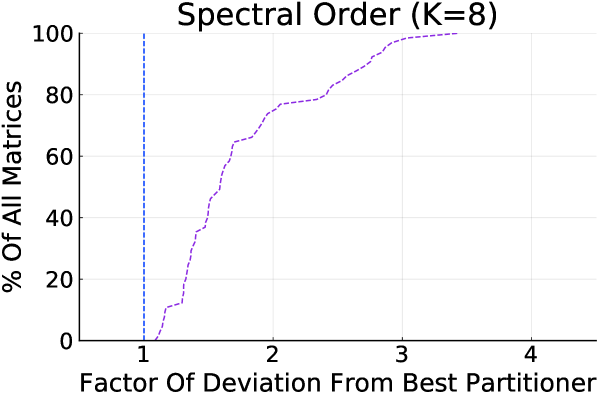
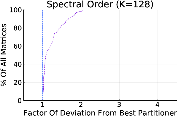
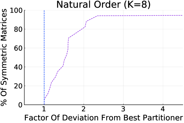
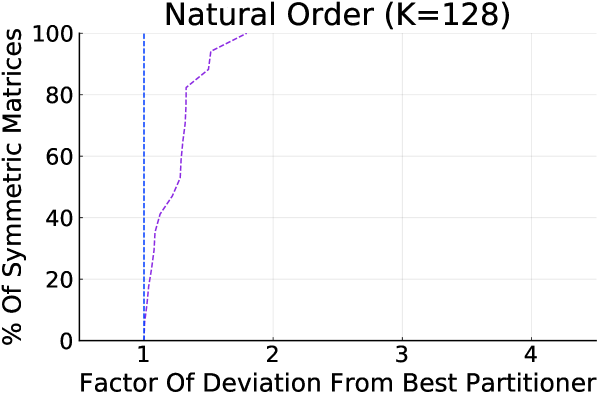
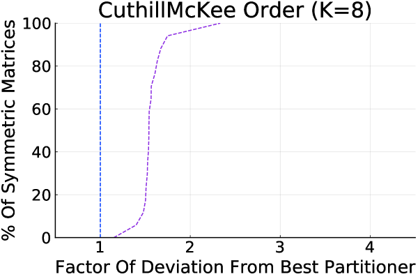
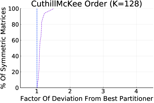
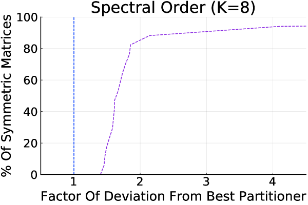
Several results are presented as performance profiles, allowing us to compare our partitioners on the entire dataset at once [58]. Partitioners are first measured by the relative deviation from the best performing partitioner for each matrix individually. We then display, for each partitioner, the fraction of test instances that achieve each target deviation from the best partitioner.
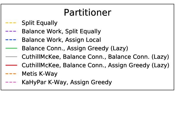
Our partitioners optimize different cost models, but we use the same coefficients whenever possible. Since the coefficients should depend on which linear solver is to be partitioned for which parallel machine, we use powers of 10 which are easy to understand and correspond to the likely orders of magnitude involved. We assume that the cost of processing one nonzero in an SpMV is . There are overheads to starting the multiplication loop in each row and several per-row costs incurred by dot products in linear solvers. We assume that the per-row cost is an order of magnitude larger; . The peak MPI bandwidth on Cori, a supercomputer at the National Energy Research Scientific Computing Center, has been measured at approximately 8 GB/s [59]. Cori uses two Intel®Xeon®Processor E5-2698 v3 CPUs on each node (one per socket). The peak computational throughput of one CPU is advertised as 1.1 TB/s (256-bit SIMD lane at 2.3 GHz on each of 16 cores). Since this is approximately two orders of magnitude faster than the communication bandwidth, we set .
The partitioners we tested are described in Table III. Our asymmetric alternating partitioners partition the primary dimension first, then partition the secondary dimension. We found that continued alternation did not significantly improve solution quality, so we do not consider partitioners which attempt to refine the initial partitioning.
All experiments were run on a single core of an Intel®Xeon®Processor E5-2695 v2 CPU running at GHz with MB of cache and GB of memory. We implemented our partitioners in Julia 1.5.1 and normalize against the Julia Standard Library SpMV; we do not expect much variation across memory-bound single-core SpMV implementations. To measure runtime, we warm up by running the kernel first, then take the minimum of at most 10,000 executions or 5 seconds worth of sampling, whichever happens first. Since some of our algorithms use randomization, we measure the average quality over 100 trials.
Partitioning represents a tradeoff between partitioning time and partition quality. Since the runtime of the partitioner must compete with the runtime of the solver, we normalize the measured serial runtime of our partitioners against the measured serial runtime of an SpMV on the same matrix. This also allows us to use aggregate runtime statistics over the whole test set.
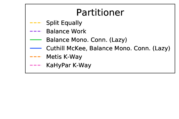
Split Equally
Assign an equal number of rows and columns to each part. Contiguous.
Balance Work
Bottleneck partition to balance load (12). Contiguous.
Assign Local
Assign each column to the part of a randomly selected incident row. Noncontiguous.
Assign Greedy Conn.
Working in random order, assign each column to a part to greedily balance bottleneck load communication (13). Noncontiguous.
Balance Mono. Conn.
Bottleneck partition to balance monotonized symmetric load communication (16). Contiguous.
Balance Conn.
Minimize Simple Cut
Total partition to minimize simple edge cut (8). Contiguous.
Minimize Hyper. Cut
Total partition to minimize hyperedge cut cost (9). Contiguous.
Minimize Conn.
Total partition to minimize cut cost (10). Contiguous.
Block Equally
Split equally into parts of cardinality . Contiguous.
Block Conn.
Split into parts of cardinality at most to minimize total cache misses (13). Contiguous.
Metis
Use direct, -way Metis with sorted heavy edge matching to optimize total edge cut (8) with a maximum of work imbalance under (12) [7]. If matrix is asymmetric, use the symmetrized bipartite representation of matrix to produce separate row and column partitions. Noncontiguous.
KaHyPar
Use direct, -way KaHyPar to optimize cut (10) with a maximum of nonzero imbalance [60]. Noncontiguous.
Spectral
Spectrally reorder. Noncontiguous.
CuthillMcKee
Reorder with Cuthill-McKee. Noncontiguous.
(Exact)
Algorithm 5 (Nicol’s Algorithm) was used to exactly bottleneck partition, and an offline dominance counter with was employed to calculate costs.
(Approx)
Algorithm 4 (Bisection) was used to -approximately bottleneck partition, and an offline dominance counter with was employed to calculate costs.
(Lazy)
Algorithm 4 (Bisection) was used to -approximately bottleneck partition, and a fused online dominance counter was employed to calculate costs.
(Dynamic)
Dynamic programming with split point bounds and constraint-based early search termination was used to solve least-weight subsequence problems for each part separately. An online dominance counter was used to calculate costs.
(Dynamic’)
Dynamic programming with split point bounds and constraint-based early search termination was used to solve simultaneous least-weight subsequence problems. An online dominance counter was used to calculate costs.
Quadrangle
Our quadrangle-accelerated algorithm with split point bounds was used to solve least-weight-subsequence subproblems for each part separately, and an offline dominance counter with was employed to calculate costs.
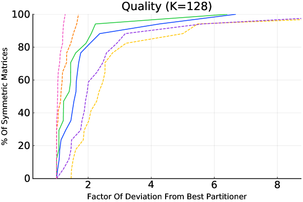
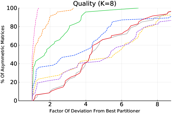
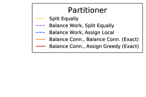
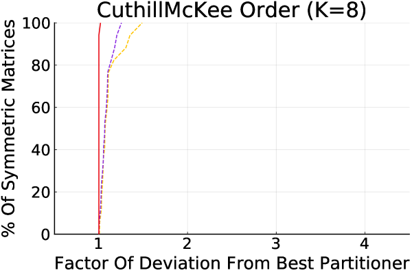
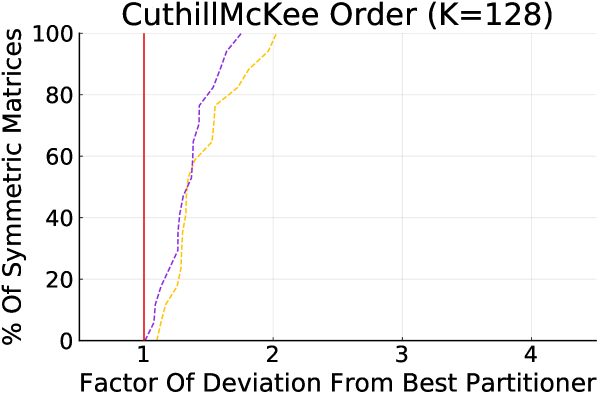
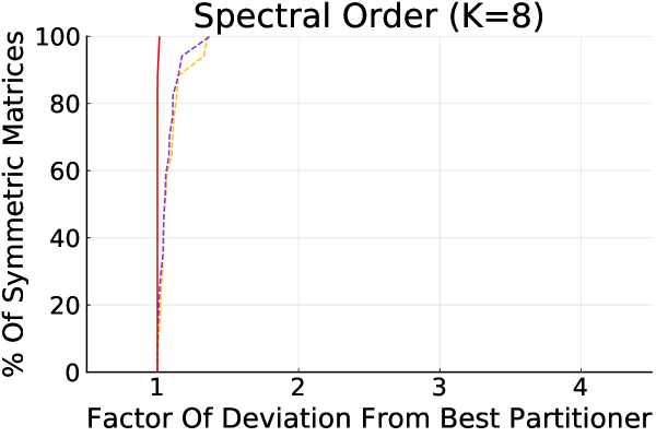
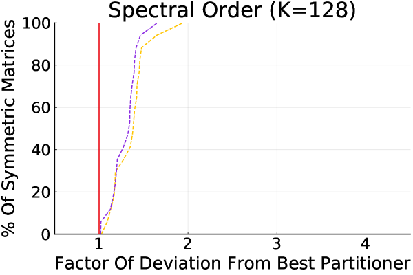
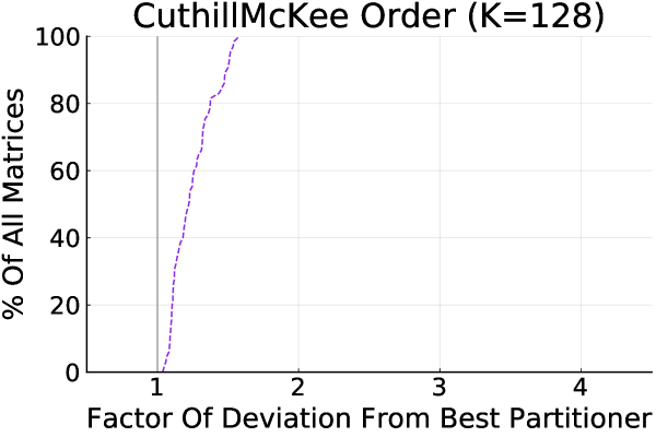
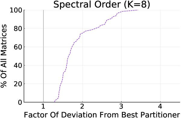
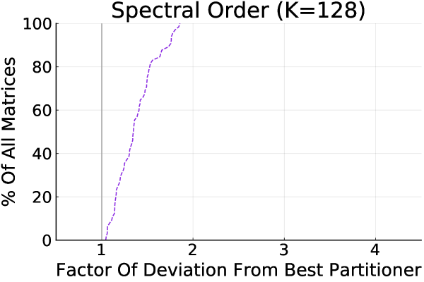
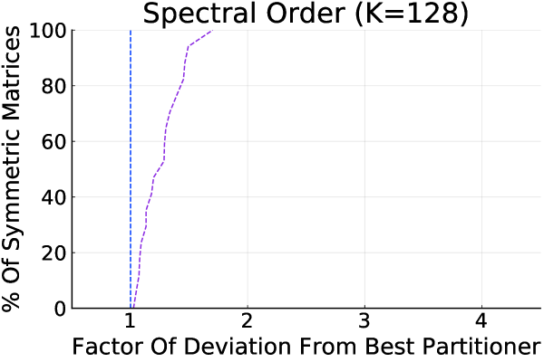
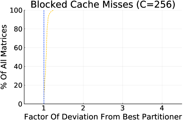
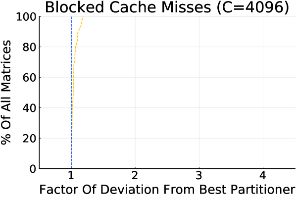
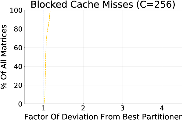
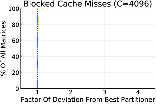
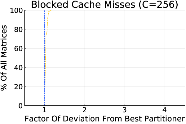
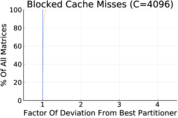
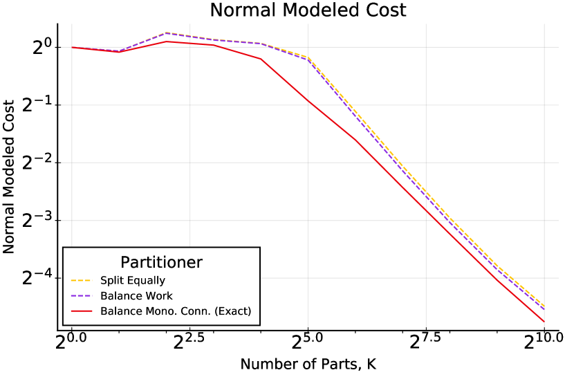
Figure 5 compares the quality of contiguous partitions under the several cost metrics we have addressed in this work. This figure shows that even in the contiguous regime, cost-aware partitioners can improve significantly over simpler strategies such as equal splitting or work balancing. The benefits were especially pronounced for bottleneck partitioning, often improving by more than a factor of . Similar benefits were observed when partitioning Cuthill-McKee or spectrally reordered symmetric matrices, but were less pronounced when was smaller, since these algorithms cluster nonzeros more evenly along the diagonal. The asymmetric bottleneck partitioner “Balance Comm, Balance Comm” constrains the second partition to be contiguous, and is therefore more competitive on these bandwidth-reduced reordered matrices where nonzeros occur in a roughly diagonal pattern. The asymmetric “Balance Comm, Assign Greedy” and “Balance Work, Assign Local” partitioners allow the column partition to be noncontiguous, and are therefore more robust to natural orderings. While our partitioners significantly improved on the quality of the equal splitting strategy, no such improvements were found when blocking to minimize cache misses.
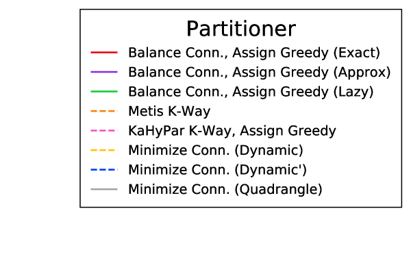
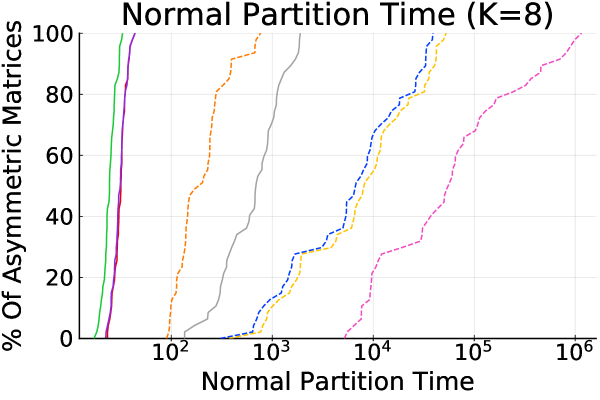
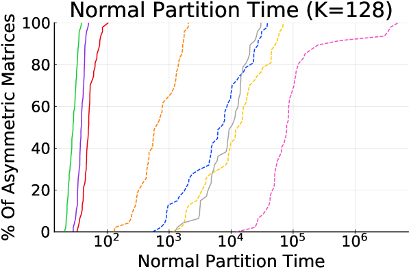
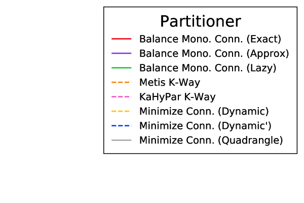
Figure 6 compares the normalized runtime of all of our partitioners. In general, the relative runtimes of these partitioners agrees with their asymptotic descriptions. Contiguous bottleneck partitioning is by far the fastest partitioning strategy, and while contiguous total hyperedge cut partitioning is much faster than general total hyperedge cut partitioning (KaHyPar), it is also slower than general simple edge cut partitioning (Metis).
When total partitioning, using offline dominance counting with and our quadrangle-accelerated algorithm was significantly faster than the dynamic programming approach with online dominance counting when the number of parts was small, but the opposite was true when was large. Note that both algorithms reduce the -partitioning problem to a sequence of least-weight subsequence problems. As becomes smaller, the average weight constraint on each part grows, and our dynamic programming algorithm endures longer split point searches. When the average weight constraint is long enough, the quadrangle algorithm’s asymptotic advantage becomes visible. Since the cache blocking problem can be solved as a single constrained least-weight subsequence problem, Figure 7 provides perspective on this effect by comparing the runtime of the dynamic programming algorithm and the quadrangle algorithm as the weight constraint grows. We see that the quadrangle algorithm begins to outperform the dynamic programming algorithm when the weight constraint exceeds about 1000 vertices. When , the dynamic, simultaneous, and quadrangle total connectivity partitioners had average runtimes of , , and SpMVs, respectively. The quadrangle algorithm resulted in a maximum speedup of and a mean speedup of over the dynamic programming algorithm.
When bottleneck partitioning, using offline dominance counting with and our linear time Algorithms 4 or 5 was efficient enough to be practical. However, for approximate partitioning, it was empirically fastest to use online dominance counters and fuse them directly into our linear search version of Algorithm 4, even though it is asymptotically slower by a factor of . The resulting pseudocode is described in Appendix A. When , the exact algorithm is expected to run in linear time when grows slower than . When , on average over our symmetric matrices, the exact, approximate, and lazy approximate algorithms were able to partition under cost (16) in an average of , , and SpMVs, respectively. The improved runtime of the linear search algorithm is due to the simplicity of the implementations, since the cost calculations are fully inlined.
General Partitioning
Bottleneck Load Connectivity On Symmetric Matrices
Bottleneck Load Connectivity On Symmetric Matrices
Contiguous Partition Quality Improvements
Bottleneck Load Connectivity On Asymmetric Matrices
 Bottleneck Load Connectivity On Symmetric Matrices
 Load Balanced Total Connectivity On All Matrices
 Load Balanced Hyperedge Cut On All Matrices
 Load Balanced Edge Cut On Symmetric Matrices
 Cache Blocked Connectivity On All Matrices
Contiguous Partitioner Runtimes
Symmetric Matrices
 Asymmetric Matrices
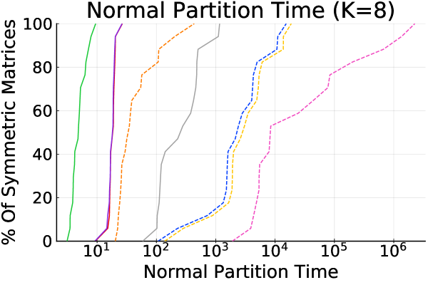
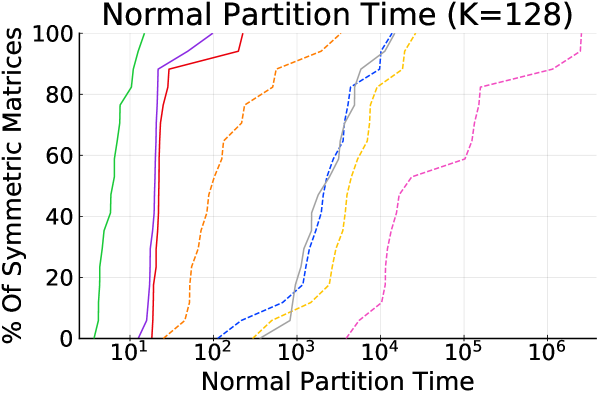
Cache Blocking Runtimes
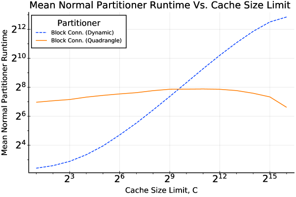
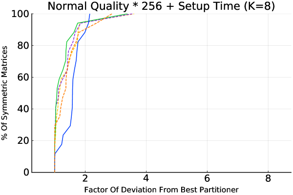
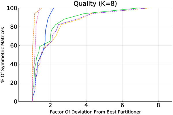
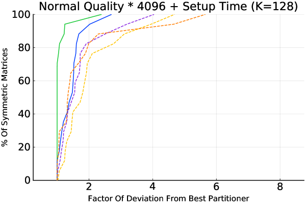
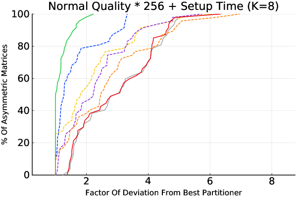
Figure 4 compares symmetric and asymmetric partitioners on our bottleneck cost in the case where the partition need not be contiguous. The figure shows that contiguous communication-aware partitioners are often competitive with reordering partitioners when we account for setup time and realistic levels of partition reuse. Furthermore, these results show that communication-aware bottleneck contiguous partitioning is more effective when the number of parts is high (and the aspect ratio of each part emphasizes communication over computation). Cuthill-McKee reordering before partitioning is only a good strategy for symmetric matrices when the number of parts is low. The KaHyPar hypergraph partitioner produced the best quality solutions, but took far too long to partition, and fell off the drawable region of the graph.
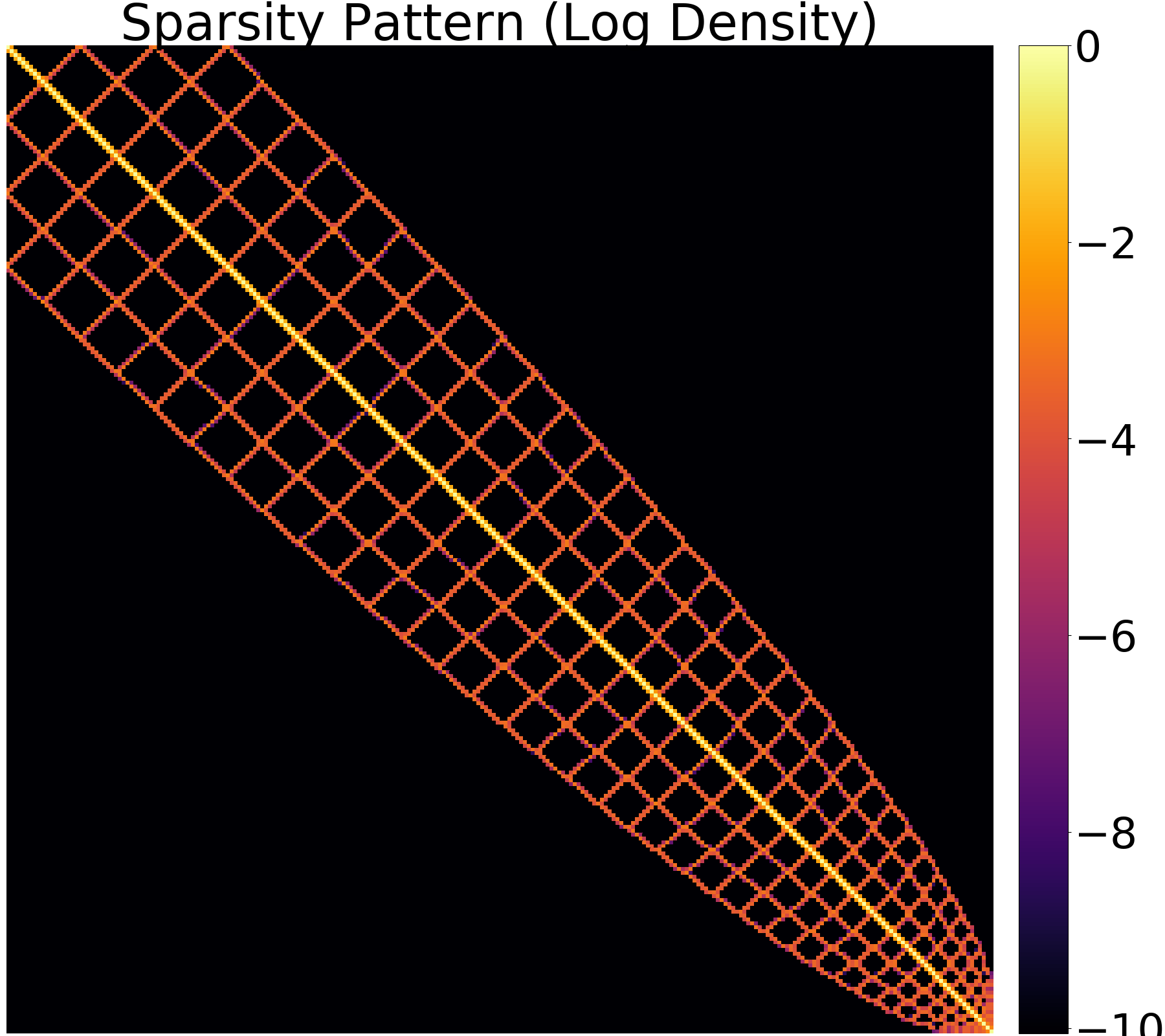
PARSEC/H2O (Symmetric Partition)
Mallya/lhr34 (Column Partition)
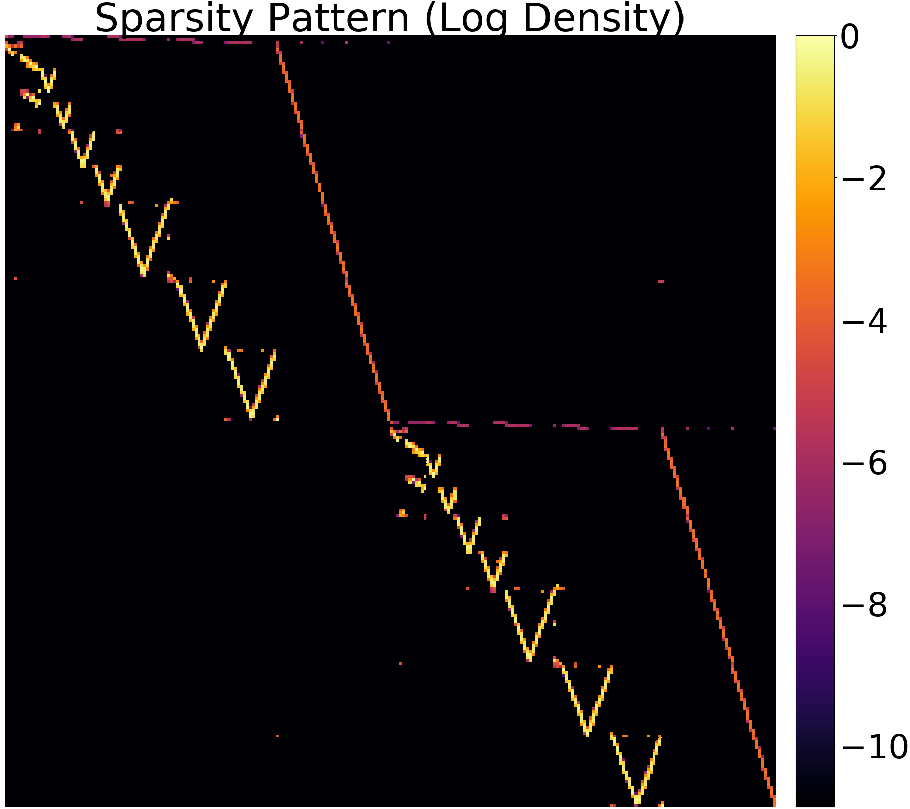
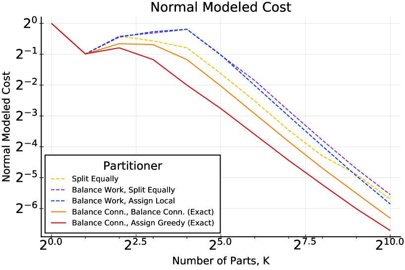
Figure 8 is meant to help give intuition for how the sparsity pattern of a matrix affects contiguous partitioning performance. Contiguous partitioning returns for PARSEC/H2O, a quantum chemistry problem, show the scale-dependence of structure utilization. For our naturally-ordered partitions, we see that increasing the number of processors does not reduce the cost until the partitions are skinny enough to resolve the structure in the matrix. Since the pattern is roughly 32 large diamonds long along the diagonal, we can only split all the diamonds at around 64 processors, which is roughly when the cost of the partitions begins to decrease in earnest. Mallya/lhr34 is a matrix arising in a nonlinear solver in a chemical process simulation. Because this matrix has a macro block structure, it is easily split into two parts in its natural ordering. However, continued bisection increases communication costs until there are enough parts to effectively split the finer structures in the matrix. Since Mallya/lhr34 is asymmetric, we can compare the effectiveness of greedy and contiguous secondary partitioning. Nonzeros occur in roughly two bands; the greedy strategy can split local rows among column parts in both bands, while the contiguous strategy suffers because the nonzeros aren’t clustered on the diagonal.
8 Conclusion
Traditional graph partitioning is NP-Hard, and only a limited set of objectives have been considered. While the ordering of the rows and columns of a matrix does not affect the meaning of the described linear operation, there are many situations where it carries useful information about the problem structure. Contiguous partitioning shifts the burden of reordering onto the user, asking them to use domain-specific knowledge or known heuristics to produce good orderings. In exchange, we show that the contiguous partitioning problem can be solved optimally in linear or near linear time and space, provably optimizing cost models which are close to the realities of distributed parallel computing.
Researchers point out that traditional graph partitioning approaches are inaccurate, since they minimize the total communication, rather than the maximum runtime of any processor under combined work and communication factors. [9, 28, 33, 26]. We show that, in the contiguous partitioning case, we can efficiently minimize the maximum runtime under the more accurate combined cost models.
We present a rich framework for constructing and optimizing expressive cost models for contiguous decompositions of iterative solvers. We describe a taxonomy of cost model properties, including convexity, monotonicity, and perhaps subadditivity. Using a set of efficiently computable “atoms”, we can construct complex “molecules” of cost functions which express complicated nonlinear dynamics such as cache effects, memory constraints, and communication costs. We adapt state-of-the-art load balancing and least-weight subsequence algorithms to optimize our costs. In order to efficiently compute our communication costs, we reduce our cost queries to dominance count queries and generalize a classical dominance counting algorithm to reduce construction time by increasing query time. Our new data structure can also be used to compute sparse prefix sums. We demonstrate that there are significant quality variations among partitioners in the contiguous setting, and that all of our algorithms efficiently produce high-quality partitions in practice.
There are several opportunities for future work. First, we discuss parallel implementations of our partitioners. Because our lazy partitioner relies on linear search to construct partitions, it does not appear to be amenable to parallelization. On the other hand, the bulk of the runtime for our binary-search-based partitioners (Algorithms 4 and 5) consists of dominance counting subroutines. As our dominance counters (Algorithms 1 and 2) are composed of decorated histogram sorts and one-dimensional prefix sums, parallelizing our dominance counters with similar strategies looks promising.
Our approaches might also be accelerated with algorithmic improvements. Since the dominance counters recursively decompose the index space, there may be opportunities to integrate dominance counting with binary search subroutines. Additionally, one might be able to approximate the computation by sampling edges or nonzeros.
References
- [1] T. F. Chan, P. Ciarlet, and W. K. Szeto, “On the Optimality of the Median Cut Spectral Bisection Graph Partitioning Method,” SIAM Journal on Scientific Computing, vol. 18, no. 3, pp. 943–948, May 1997.
- [2] K. Aydin, M. Bateni, and V. Mirrokni, “Distributed Balanced Partitioning via Linear Embedding †,” Algorithms, vol. 12, no. 8, p. 162, Aug. 2019.
- [3] S. Acer, E. G. Boman, C. A. Glusa, and S. Rajamanickam, “Sphynx: A parallel multi-GPU graph partitioner for distributed-memory systems,” Parallel Computing, p. 102769, Apr. 2021.
- [4] M. Deveci, S. Rajamanickam, K. D. Devine, and Ü. V. Çatalyürek, “Multi-Jagged: A Scalable Parallel Spatial Partitioning Algorithm,” IEEE Transactions on Parallel and Distributed Systems, vol. 27, no. 3, pp. 803–817, Mar. 2016.
- [5] J. Herrmann, J. Kho, B. Uçar, K. Kaya, and Ü. V. Çatalyürek, “Acyclic Partitioning of Large Directed Acyclic Graphs,” in 2017 17th IEEE/ACM International Symposium on Cluster, Cloud and Grid Computing (CCGRID), May 2017, pp. 371–380.
- [6] J. Herrmann, M. Y. Özkaya, B. Uçar, K. Kaya, and Ü. V. Çatalyürek, “Multilevel Algorithms for Acyclic Partitioning of Directed Acyclic Graphs,” SIAM Journal on Scientific Computing, vol. 41, no. 4, pp. A2117–A2145, Jan. 2019.
- [7] G. Karypis and V. Kumar, “A Fast and High Quality Multilevel Scheme for Partitioning Irregular Graphs,” SIAM Journal on Scientific Computing, vol. 20, no. 1, pp. 359–392, Jan. 1998.
- [8] U. V. Catalyurek and C. Aykanat, “Hypergraph-partitioning-based decomposition for parallel sparse-matrix vector multiplication,” IEEE Transactions on Parallel and Distributed Systems, vol. 10, no. 7, pp. 673–693, Jul. 1999.
- [9] B. Hendrickson, “Load balancing fictions, falsehoods and fallacies,” Applied Mathematical Modelling, vol. 25, no. 2, pp. 99–108, Dec. 2000.
- [10] E. Cuthill and J. McKee, “Reducing the bandwidth of sparse symmetric matrices,” in Proceedings of the 1969 24th national conference. Association for Computing Machinery, Aug. 1969, pp. 157–172.
- [11] A. Pothen, H. D. Simon, and K.-P. Liou, “Partitioning sparse matrices with eigenvectors of graphs,” SIAM Journal on Matrix Analysis and Applications, vol. 11, no. 3, pp. 430–452, May 1990.
- [12] A. Grandjean and B. Uçar, “On Partitioning Two Dimensional Finite Difference Meshes for Distributed Memory Parallel Computers,” in 2014 22nd Euromicro International Conference on Parallel, Distributed, and Network-Based Processing, Feb. 2014, pp. 9–16.
- [13] B. W. Kernighan, “Optimal Sequential Partitions of Graphs,” Journal of the ACM (JACM), vol. 18, no. 1, pp. 34–40, Jan. 1971.
- [14] B. Chazelle, “A Functional Approach to Data Structures and Its Use in Multidimensional Searching,” SIAM Journal on Computing, vol. 17, no. 3, pp. 427–462, Jun. 1988.
- [15] D. M. Nicol, “Rectilinear Partitioning of Irregular Data Parallel Computations,” Journal of Parallel and Distributed Computing, vol. 23, no. 2, pp. 119–134, Nov. 1994.
- [16] E. Saule, E. Ö. Baş, and Ü. V. Çatalyürek, “Load-balancing spatially located computations using rectangular partitions,” Journal of Parallel and Distributed Computing, vol. 72, no. 10, pp. 1201–1214, Oct. 2012.
- [17] A. Yaşar, M. F. Balin, X. An, K. Sancak, and Ü. V. Çatalyürek, “On Symmetric Rectilinear Matrix Partitioning,” arXiv:2009.07735 [cs], Sep. 2020.
- [18] D. Eppstein, “Sequence comparison with mixed convex and concave costs,” Journal of Algorithms, vol. 11, no. 1, pp. 85–101, Mar. 1990.
- [19] K. Akbudak and C. Aykanat, “Exploiting Locality in Sparse Matrix-Matrix Multiplication on Many-Core Architectures,” IEEE Transactions on Parallel and Distributed Systems, vol. 28, no. 8, pp. 2258–2271, Aug. 2017.
- [20] N. Abubaker, K. Akbudak, and C. Aykanat, “Spatiotemporal Graph and Hypergraph Partitioning Models for Sparse Matrix-Vector Multiplication on Many-Core Architectures,” IEEE Transactions on Parallel and Distributed Systems, vol. 30, no. 2, pp. 445–458, Feb. 2019.
- [21] M. A. Iqbal, “Approximate algorithms for partitioning problems,” International Journal of Parallel Programming, vol. 20, no. 5, pp. 341–361, Oct. 1991.
- [22] A. Pınar and C. Aykanat, “Fast optimal load balancing algorithms for 1D partitioning,” Journal of Parallel and Distributed Computing, vol. 64, no. 8, pp. 974–996, Aug. 2004.
- [23] T. G. Kolda, “Partitioning sparse rectangular matrices for parallel processing,” in Solving Irregularly Structured Problems in Parallel. Springer, 1998, pp. 68–79.
- [24] B. Hendrickson and T. G. Kolda, “Partitioning Rectangular and Structurally Unsymmetric Sparse Matrices for Parallel Processing,” SIAM Journal on Scientific Computing, vol. 21, no. 6, pp. 2048–2072, Jan. 2000.
- [25] K. D. Devine, E. G. Boman, R. T. Heaphy, R. H. Bisseling, and U. V. Catalyurek, “Parallel hypergraph partitioning for scientific computing,” in Proceedings 20th IEEE International Parallel Distributed Processing Symposium, Apr. 2006, pp. 10 pp.–.
- [26] S. Rajamanickam and E. Boman, “Parallel partitioning with Zoltan: Is hypergraph partitioning worth it?” in Contemporary Mathematics. American Mathematical Society, Jan. 2013, vol. 588, pp. 37–52.
- [27] A. Pinar and B. Hendrickson, “Partitioning for complex objectives,” in 2001 IEEE International Parallel and Distributed Processing Symposium, Apr. 2001, pp. 1232–1237.
- [28] B. Uçar and C. Aykanat, “Encapsulating Multiple Communication-Cost Metrics in Partitioning Sparse Rectangular Matrices for Parallel Matrix-Vector Multiplies,” SIAM Journal on Scientific Computing, vol. 25, no. 6, pp. 1837–1859, Jan. 2004.
- [29] K. Akbudak, O. Selvitopi, and C. Aykanat, “Partitioning Models for Scaling Parallel Sparse Matrix-Matrix Multiplication,” ACM Transactions on Parallel Computing, vol. 4, no. 3, pp. 13:1–13:34, Jan. 2018.
- [30] M. Deveci, K. Kaya, B. Uçar, and U. V. Çatalyürek, “Hypergraph Partitioning for Multiple Communication Cost Metrics,” J. Parallel Distrib. Comput., vol. 77, no. C, pp. 69–83, Mar. 2015.
- [31] S. Acer, O. Selvitopi, and C. Aykanat, “Improving performance of sparse matrix dense matrix multiplication on large-scale parallel systems,” Parallel Computing, vol. 59, pp. 71–96, Nov. 2016.
- [32] M. O. Karsavuran, S. Acer, and C. Aykanat, “Reduce Operations: Send Volume Balancing While Minimizing Latency,” IEEE Transactions on Parallel and Distributed Systems, vol. 31, no. 6, pp. 1461–1473, Jun. 2020.
- [33] R. H. Bisseling and W. Meesen, “Communication balancing in parallel sparse matrix-vector multiplication.” ETNA. Electronic Transactions on Numerical Analysis [electronic only], vol. 21, pp. 47–65, 2005.
- [34] M. R. Garey, D. S. Johnson, and L. Stockmeyer, “Some simplified NP-complete graph problems,” Theoretical Computer Science, vol. 1, no. 3, pp. 237–267, Feb. 1976.
- [35] T. Lengauer, Combinatorial algorithms for integrated circuit layout. John Wiley & Sons, Inc., 1990.
- [36] A. Grandjean, J. Langguth, and B. Uçar, “On Optimal and Balanced Sparse Matrix Partitioning Problems,” in 2012 IEEE International Conference on Cluster Computing, Sep. 2012, pp. 257–265.
- [37] G. Dósa, “The Tight Bound of First Fit Decreasing Bin-Packing Algorithm Is FFD(I) <= 11/9OPT(I) + 6/9,” in Combinatorics, Algorithms, Probabilistic and Experimental Methodologies. Springer, 2007, pp. 1–11.
- [38] D. Nicol and D. O’Hallaron, “Improved algorithms for mapping pipelined and parallel computations,” IEEE Transactions on Computers, vol. 40, no. 3, pp. 295–306, Mar. 1991.
- [39] L. H. Ziantz, C. C. Özturan, and B. K. Szymanski, “Run-time optimization of sparse matrix-vector multiplication on SIMD machines,” in PARLE’94 Parallel Architectures and Languages Europe. Springer, 1994, pp. 313–322.
- [40] M. Ashraf Iqbal and S. Bokhari, “Efficient algorithms for a class of partitioning problems,” IEEE Transactions on Parallel and Distributed Systems, vol. 6, no. 2, pp. 170–175, Feb. 1995.
- [41] C. J. Alpert and A. B. Kahng, “Splitting an Ordering into a Partition to Minimize Diameter,” Journal of Classification, vol. 14, no. 1, pp. 51–74, Jan. 1997.
- [42] Y. Saad, Iterative methods for sparse linear systems, 2nd ed. SIAM, 2003.
- [43] P. Gupta, R. Janardan, and M. Smid, “Further Results on Generalized Intersection Searching Problems: Counting, Reporting, and Dynamization,” Journal of Algorithms, vol. 19, no. 2, pp. 282–317, Sep. 1995.
- [44] H. N. Gabow, J. L. Bentley, and R. E. Tarjan, “Scaling and related techniques for geometry problems,” in Proceedings of the sixteenth annual ACM symposium on Theory of computing. Association for Computing Machinery, Dec. 1984, pp. 135–143.
- [45] P. Ahrens and E. G. Boman, “On Optimal Partitioning For Sparse Matrices In Variable Block Row Format,” arXiv:2005.12414 [cs], May 2020.
- [46] C. Alpert and A. Kahng, “Multiway partitioning via geometric embeddings, orderings, and dynamic programming,” IEEE Transactions on Computer-Aided Design of Integrated Circuits and Systems, vol. 14, no. 11, pp. 1342–1358, Nov. 1995.
- [47] J. JaJa, C. W. Mortensen, and Q. Shi, “Space-Efficient and fast algorithms for multidimensional dominance reporting and counting,” in Proceedings of the 15th international conference on Algorithms and Computation. Springer-Verlag, Dec. 2004, pp. 558–568.
- [48] T. M. Chan and B. T. Wilkinson, “Adaptive and Approximate Orthogonal Range Counting,” ACM Transactions on Algorithms, vol. 12, no. 4, pp. 45:1–45:15, Sep. 2016.
- [49] B. Chazelle, “Lower bounds for orthogonal range searching: part II. The arithmetic model,” Journal of the ACM (JACM), vol. 37, no. 3, pp. 439–463, Jul. 1990.
- [50] S. Alstrup, G. Stolting Brodal, and T. Rauhe, “New data structures for orthogonal range searching,” in Proceedings 41st Annual Symposium on Foundations of Computer Science, Nov. 2000, pp. 198–207.
- [51] M. Shekelyan, A. Dignös, and J. Gamper, “Sparse prefix sums: Constant-time range sum queries over sparse multidimensional data cubes,” Information Systems, vol. 82, pp. 136–147, May 2019.
- [52] Z. Galil and R. Giancarlo, “Speeding up dynamic programming with applications to molecular biology,” Theoretical Computer Science, vol. 64, no. 1, pp. 107–118, Apr. 1989.
- [53] M. M. Klawe and D. J. Kleitman, “An Almost Linear Time Algorithm for Generalized Matrix Searching,” SIAM Journal on Discrete Mathematics, vol. 3, no. 1, pp. 81–97, Feb. 1990.
- [54] R. Wilber, “The concave least-weight subsequence problem revisited,” Journal of Algorithms, vol. 9, no. 3, pp. 418–425, Sep. 1988.
- [55] M. Manguoglu, A. H. Sameh, and O. Schenk, “PSPIKE: A Parallel Hybrid Sparse Linear System Solver,” in Euro-Par 2009 Parallel Processing. Springer, 2009, pp. 797–808.
- [56] W. M. Chan and A. George, “A linear time implementation of the reverse Cuthill-McKee algorithm,” BIT Numerical Mathematics, vol. 20, no. 1, pp. 8–14, Mar. 1980.
- [57] M. W. Berry, B. Hendrickson, and P. Raghavan, “Sparse Matrix Reordering Schemes for Browsing Hypertext,” in The Mathematics of Numerical Analysis. American Mathematical Society, 1996, vol. 32, pp. 99–122.
- [58] E. D. Dolan and J. J. Moré, “Benchmarking optimization software with performance profiles,” Mathematical Programming, vol. 91, no. 2, pp. 201–213, Jan. 2002.
- [59] D. Doerfler, B. Austin, B. Cook, J. Deslippe, K. Kandalla, and P. Mendygral, “Evaluating the networking characteristics of the Cray XC-40 Intel Knights Landing-based Cori supercomputer at NERSC,” Concurrency and Computation: Practice and Experience, vol. 30, no. 1, p. e4297, 2018.
- [60] L. Gottesbüren, M. Hamann, S. Schlag, and D. Wagner, “Advanced Flow-Based Multilevel Hypergraph Partitioning,” in 18th International Symposium on Experimental Algorithms (SEA 2020), vol. 160. Schloss Dagstuhl–Leibniz-Zentrum für Informatik, 2020, pp. 11:1–11:15.
![[Uncaptioned image]](/html/2007.16192/assets/IMG_6762.jpeg) |
Peter Ahrens is Department of Energy Computational Science Graduate Fellow working towards a Ph.D. in computer science at the Massachusetts Institute of Technology under the supervision of Professor Saman Amarasinghe. Peter completed his B.S. in computer science and minor in mathematics at the University of California, Berkeley. His research interests include graph algorithms, compilers, numerical analysis, and high performance computing with applications in scientific computing. |
Appendix A Lazy Probe Pseudocode
Algorithm 6 details pseudocode for the lazy probe algorithm described in Section 5. The algorithm computes the atoms needed for all of our cost functions in primary or symmetric partitioning settings.
Algorithm 6 (Lazy BISECT Partitioner).
Given a cost function(s) defined on the atoms , , , , , and , which is monotonic increasing in , find a contiguous -partition which minimizes
to a relative accuracy of within the range , if such a partition exists.
This algorithm differs from Algorithm 4 only in the probe function, so we only describe the new LazyProbe pseudocode. We assume that .