On the two-dimensional knapsack problem for convex polygons
Abstract.
We study the two-dimensional geometric knapsack problem for convex polygons. Given a set of weighted convex polygons and a square knapsack, the goal is to select the most profitable subset of the given polygons that fits non-overlappingly into the knapsack. We allow to rotate the polygons by arbitrary angles. We present a quasi-polynomial time -approximation algorithm for the general case and a polynomial time -approximation algorithm if all input polygons are triangles, both assuming polynomially bounded integral input data. Also, we give a quasi-polynomial time algorithm that computes a solution of optimal weight under resource augmentation, i.e., we allow to increase the size of the knapsack by a factor of for some but compare ourselves with the optimal solution for the original knapsack. To the best of our knowledge, these are the first results for two-dimensional geometric knapsack in which the input objects are more general than axis-parallel rectangles or circles and in which the input polygons can be rotated by arbitrary angles.
1. Introduction
In the two-dimensional geometric knapsack problem (2DKP) we are given a square knapsack for some integer and a set of convex polygons where each polygon has a weight ; we write for any set . The goal is to select a subset of maximum total weight such that the polygons in fit non-overlapping into if we translate and rotate them suitably (by arbitrary angles). 2DKP is a natural packing problem, the reader may think of cutting items out of a piece of raw material like metal or wood, cutting cookings out of dough, or, in three dimensions, loading cargo into a ship or a truck. In particular, in these applications the respective items can have various kinds of shapes. Also note that 2DKP is a natural geometric generalization of the classical one-dimensional knapsack problem.
Our understanding of 2DKP highly depends on the type of input objects. If all polygons are axis-parallel squares there is a -approximation with a running time of the form (i.e., an EPTAS) [HW19], and there can be no FPTAS (unless ) since the problem is strongly -hard [LTW+90]. For axis-parallel rectangles there is a polynomial time -approximation algorithm and a -approximation if the items can be rotated by exactly 90 degrees [GGH+17]. If the input data is quasi-polynomially bounded there is even a -approximation in quasi-polynomial time [AW15], with and without the possibility to rotate items by 90 degrees. For circles a -approximation is known under resource augmentation in one dimension if the weight of each circle equals its area [LMX18].
To the best of our knowledge, there is no result known for 2DKP for shapes different than axis-parallel rectangles and circles. Also, there is no result known in which input polygons are allowed to be rotated by angles different than 90 degrees. However, in the applications of 2DKP the items might have shapes that are more complicated than rectangles or circles. Also, it makes sense to allow rotations by arbitrary angles, e.g., when cutting items out of some material. In this paper, we present the first results for 2DKP in these settings.
1.1. Our contribution
We study 2DKP for arbitrary convex polygons, allowing to rotate them by arbitrary angles. Note that due to the latter, it might be that some optimal solution places the vertices of the polygons on irrational coordinates, even if all input numbers are integers. Our first results are a quasi-polynomial time -approximation algorithm for general convex polygons and a polynomial time -approximation algorithm for triangles.
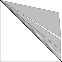
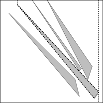
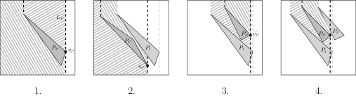
By rotation we can assume for each input polygon that the line segment defining its diameter is horizontal. We identify three different types of polygons for which we employ different strategies for packing them, see Figure 1a). First, we consider the easy polygons which are the polygons whose bounding boxes fit into the knapsack without rotation. We pack these polygons such that their bounding boxes do not intersect. Using area arguments and the Steinberg’s algorithm [Ste97] we obtain a -approximation for the easy polygons. Then we consider the medium polygons which are the polygons whose bounding boxes easily fit into the knapsack if we can rotate them by 45 degrees. We use a special type of packing in which the bounding boxes are rotated by 45 degrees and then stacked on top of each other, see Figure 1b). More precisely, we group the polygons by the widths of their bounding boxes and to each group we assign two rectangular containers in the packing. We compute the essentially optimal solution of this type by solving a generalization of one-dimensional knapsack for each group. Our key structural insight for medium polygons is that such a solution is -approximate. To this end, we prove that in the medium polygons of each group occupy an area that is by at most a constant factor bigger than the corresponding containers, and that a constant fraction of these polygons fit into the containers. In particular, we show that medium polygons with very wide bounding boxes lie in a very small hexagonical area close to the diagonal of the knapsack. Our routines for easy and medium polygons run in polynomial time.
It remains to pack the hard polygons whose bounding boxes just fit into the knapsack or do not fit at all, even under rotation. Note that this does not imply that the polygon itself does not fit. Our key insight is that there can be only such polygons in the optimal solution, at most from each group. Therefore, we can guess these polygons in quasi-polynomial time, assuming that is quasi-polynomially bounded. However, in contrast to other packing problems, it is not trivial to check whether a set of given polygons fits into the knapsack since we can rotate them by arbitrary angles and we cannot enumerate all possibilities for the angles. However, we show that by losing a constant factor in the approximation guarantee we can assume that the placement of each hard polygon comes from a precomputable polynomial size set and hence we can guess the placements of the hard polygons in quasi-polynomial time.
Theorem 1.
There is a -approximation algorithm for 2DKP with a running time of .
 |
 |
 |
| (a) | (b) | (c) |

If all hard polygons are triangles we present even a polynomial time -approximation algorithm. We split the triangles in into two types, for one type we show that a constant fraction of it can be packed in what we call top-left-packings, see Figure 1b). In these packings, the triangles are sorted by the lengths of their longest edges and placed on top of each other in a triangular area. We devise a dynamic program (DP) that essentially computes the most profitable top-left-packing. For proving that this yields a -approximation, we need some careful arguments for rearranging a subset of the triangles with large weight to obtain a packing that our DP can compute. We observe that essentially all hard polygons in must intersect the horizontal line that contains the mid-point of the knapsack. Our key insight is that if we pack a triangle in a top-left-packing then it intersects this line to a similar extent as in . Then we derive a sufficient condition when a set of triangles fits in a top-left-packing, based on by how much they overlap this line.
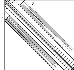
For the other type of triangles we use a geometric dynamic program. In this DP we recursively subdivide the knapsack into subareas in which we search for the optimal solution recursively, see Figure 1c). In the process we guess the placements of some triangles from . Again, by losing a constant factor we can assume that for each triangle in there are only a polynomial number of possible placements. By exploiting structural properties of this type of triangles we ensure that the number of needed DP-cells is bounded by a polynomial. A key difficulty is that we sometimes split the knapsack into two parts on which we recurse independently. Then we need to ensure that we do not select some (possibly high weight) triangle in both parts. To this end, we globally select at most one triangle from each of the groups (losing a constant factor) and when we recurse, we guess for each subproblem from which of the groups it contains a triangle in . This yields only guesses.
Theorem 2.
There is a -approximation algorithm for 2DKP with a running time of if all input polygons are triangles.
Then we study the setting of resource augmentation, i.e., we compute a solution that fits into a larger knapsack of size for some constant and compare ourselves with a solution that fits into the original knapsack of size . We show that then the optimal solution can contain only constantly many hard polygons and hence we can guess them in polynomial time.
Theorem 3.
There is a -approximation algorithm for 2DKP under -resource augmentation with a running time of .
Finally, we present a quasi-polynomial time algorithm that computes a solution of weight at least (i.e., we do not lose any factor in the approximation guarantee) that is feasible under resource augmentation. This algorithm does not use the above classification of polygons into easy, medium, and hard polygons. Instead, we prove that if we can increase the size of the knapsack slightly we can ensure that for the input polygons there are only different shapes by enlarging the polygons suitably. Also, we show that we need to allow only a polynomial number of possible placements and rotations for each input polygon, without sacrificing any polygons from . Then we use a technique from [AW14] implying that there is a balanced separator for the polygons in with only edges and which intersects polygons from with only very small area. We guess the separator, guess how many polygons of each type are placed inside and outside the separator, and then recurse on each of these parts. Some polygons are intersected by the balanced separator. However, we ensure that they have very small area in total and hence we can place them into the additional space of the knapsack that we gain due to the resource augmentation. This generalizes a result in [AW15] for axis-parallel rectangles.
Theorem 4.
There is an algorithm for 2DKP under -resource augmentation with a running time of that computes a solution of weight at least .
In our approximation algorithms, we focus on a clean exposition of our methodology for obtaining -approximations, rather than on optimizing the actual approximation ratio.
1.2. Other related work
Prior to the results mentioned above, polynomial time -approximation algorithms for 2DKP for axis-parallel rectangles were presented by Jansen and Zhang [JZ04b, JZ04a]. For the same setting, a PTAS is known under resource augmentation in one dimension [JSO07] and a polynomial time algorithm computing a solution with optimum weight under resource augmentation in both dimensions [HW19]. Also, there is a PTAS if the weight of each rectangle equals its area [BCJ+09]. For squares, Jansen and Solis-Oba presented a PTAS [JSO08].
2. Constant factor approximation algorithms
In this section we present our quasi-polynomial time -approximation algorithm for general convex polygons and our polynomial time -approximation algorithm for triangles., assuming polynomially bounded input data. Our strategy is to partition the input polygons into three classes, easy, medium, and hard polygons, and then to devise algorithms for each class separately.
Let denote the given knapsack. We assume that each input polygon is described by the coordinates of its vertices which we assume to be integral. First, we rotate each polygon in such that its longest diagonal (i.e., the line segment that connects the two vertices of largest distance) is horizontal. For each polygon denote by the new coordinates of its vertices. Observe that due to the rotation, the resulting coordinates might not be integral, and possibly not even rational. We will take this into account when we define our algorithms. For each we define its bounding box to be the smallest axis-parallel rectangle that contains . Formally, we define . For each polygon let and . If necessary we will work with suitable estimates of these values later, considering that they might be irrational and hence we cannot compute them exactly.
We first distinguish the input polygons into easy, medium, and hard polygons. We say that a polygon is easy if fits into without rotation, i.e., such that and . Denote by the set of easy polygons. Note that the bounding box of a polygon in might still fit into if we rotate it suitably. Intuitively, we define the medium polygons to be the polygons whose bounding box fits into with quite some slack if we rotate properly and the hard polygons are the remaining polygons (in particular those polygons whose bounding box does not fit at all into ).
Formally, for each polygon we define . The intuition for is that a rectangle of width and height is the highest rectangle of width that still fits into .
Lemma 5.
Let . A rectangle of width and height fits into (if we rotate it by 45°) but a rectangle of width and of height larger than does not fit into .
Proof.
We begin by proving that the rectangle fits into when rotating by 45o. To this end, just consider the placement of by its new vertices , , , .
We now prove the second part of the Lemma. Choose maximal such that fits into . We aim to prove that . By maximality of we can assume that in the placement into some vertex of lies on a side of . Without loss of generality we assume that lies on . Therefore for some . Draw the two lines that start in and have difference with the side . Note that these lines intersect at and , additionally and . Since fits, these are also upper bounds on and respectively. We conclude that and therefore:
concluding that and the proof of the Lemma. ∎
Hence, if is much smaller than then fits into with quite some slack. Therefore, we define that a polygon is medium if and hard otherwise. Denote by and the medium and hard polygons, respectively. We will present -approximation algorithms for each of the sets separately. The best of the computed sets will then yield a -approximation overall.
For the easy polygons, we construct a polynomial time -approximation algorithm in which we select polygons such that we can pack their bounding boxes as non-overlapping rectangles using Steinberg’s algorithm [CGJT80], see Section 2.1. The approximation ratio follows from area arguments.
Lemma 6.
There is a polynomial time algorithm that computes a solution with .
For the medium polygons, we obtain a -approximation algorithm using a different packing strategy, see Section 2.2.
Lemma 7.
There is an algorithm with a running time of that computes a solution with .
The most difficult polygons are the hard polygons. First, we show that in quasi-polynomial time we can obtain a -approximation for them, see Section 2.3.
Lemma 8.
There is an algorithm with a running time of that computes a solution with .
Combining Lemmas 6, 7, and 8 yields Theorem 1. If all polygons are triangles, we obtain a -approximation even in polynomial time. The following lemma is proved in Section 2.4 and together with Lemmas 6 and 7 implies Theorem 2.
Lemma 9.
If all input polygons are triangles, then there is an algorithm with a running time of that computes a solution with .
Orthogonal to the characterization into easy, medium and hard polygons, we subdivide the polygons in further into classes according to the respective values . More precisely, we do this according to their difference between and the diameter of , i.e., . Formally, for each we define and additionally . Note that for each polygon we can compute the group even though might be irrational.
2.1. Easy polygons
We present a -approximation algorithm for the polygons in . First, we show that the area of each polygon is at least half of the area of its bounding box. We will use this later for defining lower bounds using area arguments.
Lemma 10.
For each it holds that .
Proof.
If is a triangle the result is clear. Suppose that has more than three sides and call its longest diagonal. Split into two polygons by . Call and the triangles formed by and the vertices further away from in and respectively. By convexity we know that and . We conclude by noting that . ∎
On the other hand, it is known that we can pack any set of axis-parallel rectangles into , as long as their total area is at most and each single rectangle fits into .
Theorem 11 ([Ste97]).
Let be a set of axis-parallel rectangles such that and each individual rectangle fits into . Then there is a polynomial time algorithm that packs into .
We first compute (essentially) the most profitable set of polygons from whose total area is at most via a reduction to one-dimensional knapsack.
Lemma 12.
In time we can compute a set of polygons such that and .
Proof.
We define an instance of one-dimensional knapsack with a set of items where we introduce for each polygon an item with size and profit and define the size of the knapsack to be . We apply the FPTAS in [Jin19] on this instance and obtain a set of items such that where denote the optimal solution for the set of items , given a knapsack of size . We define . ∎
The idea is now to partition into at most 7 sets . Hence, one of these sets must contain at least a profit of . We define this partition such that each set contains only one polygon or its polygons have a total area of at most .
Lemma 13.
Given a set with . In polynomial time we can compute a set with and additionally or .
Proof.
Note that every set of rectangles that fit into the Knapsack with total area less than can be packed into the Knapsack by Theorem 11. Therefore, any set polygons of total area less than can be put into their bounding boxes and, since the total area of these boxes has at most doubled, the convex polygons can be packed accordingly. Moreover if the height and width of the bounding box can be computed in polynomial time, this placement can also be computed in polynomial time.
Sort decreasingly by area and define , and . We now partition obtaining parts as follows. We begin by defining a sequence of :
and consider the partition of into parts of the form . Suppose for the sake of contradiction that . Note that for each such that , therefore:
arriving at a contradiction. Pick the part with largest weight, therefore and, by construction, either is a single polygon that fits or has area at most and can be placed non-overlappingly into the Knapsack. ∎
If we simply pack the single polygon in into the knapsack. Otherwise, using Lemmas 10 and 12 and Theorem 11 we know that we can pack the bounding boxes of the polygons in into . Note that their heights and widths might be irrational. Therefore, we slightly increase them such that these values become rational, before applying Theorem 11 to compute the actual packing. If as a result the total area of the bounding boxes exceeds we partition them into two sets where each set satisfies that the total area of the bounding boxes is at most or it contains only one polygon and we keep the more profitable of these two sets (hence losing a factor of 2 in the approximation ratio). This yields a -approximation algorithm for the easy polygons and thus proves Lemma 6.
2.2. Medium polygons
We describe a -approximation algorithm for the polygons in . In its solution, for each we will define two rectangular containers for polygons in , each of them having width and height , see Figures 2. Let . First, we show that we can pack all containers in into (if we rotate them by 45°).
Lemma 14.
The rectangles in can be packed non-overlappingly into .
Proof.
Let be the largest integer such that . For we place the rectangle such that its vertices are at the following coordinates: , , , . Note that since:
this is indeed the rectangle .
To prove that these are placed non-overlappingly, we define a family of hyperplanes such that for each , and are in different half-spaces defined by . Define these half-spaces as:
Note that and . Therefore, if we have that and , making this a non-overlapping packing.
Noting that the rectangles are packed in the half-space , we can pack the rectangles symmetrically. ∎
For each we will compute a set of polygons of large weight. Within each container we will stack the bounding boxes of the polygons in on top of each other and then place the polygons in in their respective bounding boxes, see Figure 2. In particular, a set of items fits into (or ) using this strategy if and only if . Observe that for a polygon with it is not necessarily true that and hence for hard polygons this strategy is not suitable. We compute the essentially most profitable set of items that fits into and with the above strategy. For this, we need to solve a variation of one-dimensional knapsack with two knapsacks (instead of one) that represent and . The value for a polygon might be irrational, therefore we work with a -estimate of instead. This costs only a factor in the approximation guarantee.
Lemma 15.
Let . For each there is an algorithm with a running time of that computes two disjoint sets such that and and for any disjoint sets such that and .
Proof.
First, for each polygon we compute an estimate for that overestimates the true value for by at most a factor . Working with this estimate instead of the real value for loses at most a factor of in the profit.
For each , note that we aim to solve a variation of one-dimensional knapsack with two identical knapsacks instead of one. In our setting we have two knapsacks and , each with capacity , the set of objects to choose from are and each has size and profit . This can be done with the algorithm in [CK00]. ∎
For each with we apply Lemma 15 and obtain sets . We pack into and into , using that and . Then we pack all containers for each into , using Lemma 14.
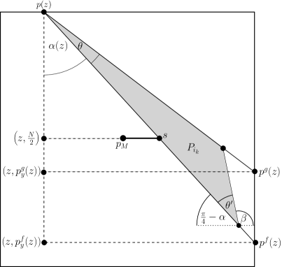
Let denote the selected polygons. We want to show that has large weight; more precisely we want to show that . First, we show that for each the polygons in have bounded area. To this end, we show that they are contained inside a certain (irregular) hexagon (see Figure 2) which has small area if the polygons are wide, i.e., if is close to . The reason is that then must be placed close to the diagonal of the knapsack and on the other hand is relatively small (since is medium), which implies that all of lies close to the diagonal of the knapsack. For any object we define to be its area.
Lemma 16.
For each it holds that .
Proof.
We show that we can choose a constant such that if a polygon is placed in the knapsack, then it is contained in the (irregular) hexagon that we define to be the hexagon with vertices , or in the (irregular) hexagon that we define to be the hexagon with vertices , see Figure 2. To prove this, we first show that in the placement of inside the vertices of the longest diagonal of essentially lie near opposite corners of . We then use this to show that this longest diagonal of lies inside one of two hexagons that are even smaller than and , respectively, see Figure 2. If additionally we conclude that is placed completely within (while if the latter is not necessarily true).
Given a value we define as the union of the triangles with vertices and and . Note that . Similarly, we define as the union of the triangles with vertices and and , noting that .
Claim.
Consider a polygon . Let be a placement of inside and let denote the longest diagonal of for two vertices of . Define . If then it holds that or . If additionally then or .
Proof of claim..
We can assume that since otherwise . Call the polygon with vertices . Note that since is a polyhedron, its diameter is given by the two vertices furthest apart. Therefore:
Hence, or . Assume w.l.o.g. that . Furthermore, assume that and assume w.l.o.g. that is contained in the triangle with vertices .
Call the hexagon with vertices , , , , , . Note that since is a polyhedron, its diameter is given by the two vertices furthest apart. Therefore . Therefore, must lie inside the triangles with vertices or inside the triangle with vertices . If lies in the latter triangle, then which is a contradiction. Therefore, . This implies that . Assume now additionally that . Let be a vertex of with . The distance between and is at most . Therefore, is contained in and hence .
The case that can be handled similarly and in this case we conclude that , , and . ∎
We choose and note that for every placement of we have that or as . Furthermore the area of (and hence the area of ) is upper bounded as follows:
Note that we can compute by computing twice the area of half the hexagon: i.e. the quadrilateral , , and , we now divide this quadrilateral into two isosceles right triangles with hypotenuse and a rectangle with sides and , obtaining the following:
More generally if we can compute by computing twice the area of the quadrilateral , , , , and doing the same splitting into triangles and rectangles we get:
We can now compute the area of
Using this, we can partition into at most subsets such that for each subset it holds that and hence fits into (and ) using our packing strategy above. Here we use that each medium polygon satisfies that .
Lemma 17.
For each there are disjoint set with such that and .
Proof.
We begin by partitioning into groups such that each group fits into . To do so, define a sequence such that:
Consider now the partition of into parts of the form . Recall that . Since , for we have . Therefore:
concluding that . Call and the most profitable parts of the partition. Using our bound on we get:
2.3. Hard polygons
We first show that for each class there are at most a constant number of polygons from in , and that for only classes it holds that .
Lemma 18.
For each it holds that . Also, if then with and .
Proof.
Recall that . Hence, if then and therefore since all polygons with satisfy that and hence .
Note that must be a positive integer. Then it is sufficient to prove that if , then is empty. We prove the stronger claim that . Note that:
From which we conclude.
We now prove the second part of the lemma by breaking the polygons into two sets. Define as the polygons that fit completely into as in Claim Claim and as . We begin with the polygons in . Recall that by Lemma 10 using additionally that we get:
Therefore:
Additionally, by Lemma 16 we have that . Combining these two, and recalling that by the first part of the Lemma we may assume that we get:
We now deal with note that has two connected components, we show that in each one there is at most one polygon intersecting it. These two are exactly the triangle with vertices , , and with vertices , and .
Suppose for the sake of contradiction that there exist points belonging to some polygons and . Let and be the diagonals of and respectively. Let and be as in Claim Claim and define . By the same Claim we get . We now consider the rays for , . Note that since , then and don’t intersect , but by convexity of and they must intersect and . Note that intersects first and then (otherwise and would be intersecting) and intersects first and then . Therefore and intersect and in different order, which means that and must intersect, a contradiction. ∎
We describe now a quasi-polynomial time algorithm for hard polygons, i.e., we want to prove Lemma 8. Lemma 18 implies that . Therefore, we can enumerate all possibilities for in time . For each for each enumerated set we need to check whether it fits into . We cannot try all possibilities for placing into since we are allowed tof rotate the polygons in by arbitrary angles. To this end, we show that there is a subset of of large weight which contains only a single polygon or it does not use the complete space of the knapsack but leaves some empty space. We use this empty space to move the polygons slightly and rotate them such that each of them is placed in one out of different positions that we can compute beforehand. Hence, we can guess all positions of these polygons in time . We define that a placement of a polygon inside is a polygon such that where and is the polygon that we obtain when we rotate by an angle clockwise around its first vertex.
Lemma 19.
For each polygon we can compute a set of possible placements in time such that there exists a set with which can be packed into such that each polygon is packed according to a placement in .
Proof.
Let to be defined later. First, we observe that there can be only classes containing polygons whose respective values are not larger than ; recall that is the length of the diagonal of .
Proposition 20.
For each there is a constant such that each polygon satisfies that .
Due to Lemma 18 there can be only hard polygons in . Hence, it suffices to prove the claim for the hard polygons in . Since for each polygon it holds that we have that in any placement of inside the line segment defining (i.e., the line segment connecting the two vertices of with maximum distance) has to have essentially a 45°angle with the edges of the knapsack.
Let denote the line segment connecting , and . Let denote the line segment connecting and , and let denote the line segment connecting and (see Figure 3). By losing a factor 3 we can assume that each polygon in intersects but not . We group the polygons in into three groups . We define that contains the polygons in that have empty intersection with . We define that contains the polygons in that have empty intersection with . Finally, we define .
Consider the group . If is sufficiently small then every polygon in intersects . We sort the polygons in in the order in which they intersect from left to right, let denote this ordering. For each we now translate each polygon to the left by units. We argue that between any two consecutive polygons there is some empty space that intuitively we can use as slack. Since are convex, for their original placement there is a line that separates them. If is sufficiently small, then the line segments defining and have essentially a 45°angle with the edges of the knapsack. Since and this implies that also also essentially forms a 45°angle with the edges of the knapsack. After translating and we can draw not only line separating them (like ) but instead a strip separating them, defined via two lines whose angle is identical to the angle of , and such that the distance between and is at least . Next, we rotate around one of its vertices until the angle of the line segment defining is a multiple of for some small constant to be defined later, or one of the vertices of touches an edge of the knapsack. In the latter case, let be a vertex of that now touches an edge of the knapsack. We rotate around until the angle of the line segment defining is a multiple of or another vertex of touches an edge of the knapsack. In the latter case we observe that two vertices of touch an edge of the knapsack. Since has at most vertices, there are at most such orientations for . Otherwise, there are only possibilities for the angle of the line segment defining which gives at most possible orientations for in total. Finally, we move to the closest placement with the property that the first vertex of is placed on a position in which both coordinates are multiples of . One can show that due to the empty space between any two consecutive polygons no two polygons overlap after the movement, if is chosen sufficiently small. This yields a placement for the polygons in in which each polygon is placed according to one out of positions.
We use a symmetric argumentation for the polygons in . Finally, we want to argue that . Observe that each polygon intersects , the stripe , the stripe , but has empty intersection with . Hence, the line segment defining must have length at least . Therefore, or with and then . First assume that . If is a sufficiently large constant we have that which contradicts Lemma 18. On the other hand, if then the claim is trivially true since then . Otherwise, assume that . By Lemma 18 there can be at most polygons from in . ∎
This yields the proof of Lemma 8.
2.4. Hard triangles
In this section we present a -approximation algorithm in polynomial time for hard polygons assuming that they are all triangles, i.e., we prove Lemma 9. Slightly abusing notation, denote by the set obtained by applying Lemma 19. We distinguish the triangles in into two types: edge-facing triangles and corner-facing triangles. Let , let denote the two longest edges of , and let the vertex of adjacent to and . Let and be the two rays that originate at and that contain and , respectively, in the placement of in . We have that and intersect at most one edge of the knapsack each. If and intersect the same edge of the knapsack then we say that is edge-facing, if one of them intersects a horizontal edge and the other one intersects a vertical edge we say that is corner-facing. The next lemma shows that there can be only triangles in that are neither edge- nor corner-facing, and therefore we compute a -approximation with respect to the total profit of such triangles by simply selecting the input triangle with maximum weight.
Lemma 21.
There can be at most triangles in that are neither edge-facing nor corner-facing.
Proof.
Let that is neither edge-facing nor corner-facing. Assume w.l.o.g. that both and intersect a horizontal edge of the knapsack. Let denote the two longest edges of . Since is hard, we know that one of these edges is longer than and therefore the other one is longer than . Let denote the angle between and . It holds that cannot be arbitrarily small since otherwise it cannot be that and intersect different horizontal edges of the knapsack. Formally, assume w.l.o.g. that lies in the upper half of the knapsack and that intersects the bottom edge of the knapsack. Let denote the angle between the horizontal line going through and (note that ). Then one can show that and thus . Therefore, . Hence, there can be at most triangles in that are neither edge-facing nor corner-facing. ∎
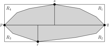
Let , , , and denote the top left, top right, bottom left, and bottom right corners of , respectively, and let , , and , see Figure 3. By losing a factor we assume from now on that that contains at most one hard triangle from each group , using Lemma 18.
Let denote the edge-facing hard triangles in and denote by the corner-facing hard triangles in . In the remainder of this section we present now -approximation algorithms for edge-facing and for corner-facing triangles in . By selecting the best solution among the two we obtain the proof of Lemma 9.
2.4.1. Edge-facing triangles
We define a special type of solutions called top-left-packings that our algorithm will compute. We will show later that there are solutions of this type whose profit is at least a constant fraction of the profit of .
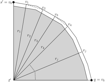
For each let . Let be a set of triangles that are ordered according to the groups , i.e., such that for any with and for some it holds that . We define a placement of that we call a top-left-packing. First, we place such that concides with and one edge of lies on the diagonal of that connects and . Note that there is a unique way to place in this way. Iteratively, suppose that we have packed triangles such that for each triangle in this set its respective vertex coincides with , see Figure 1c). Intuitively, we pack on top of such that coincides with . Let be the smallest integer such that the line segment connecting and has empty intersection with each triangle according to our placement. We place such that concides with and one of its edges lies on the line that contains and . There is a unique way to place in this way. We continue until we placed all triangles in . If all of them are placed completely inside we say that the resulting solution is a top-left-packing and that is top-left-packable. We define bottom-right-packing and bottom-right-packable symmetrically, mirroring the above definition along the line that contains and .
In the next lemma, we show that there is always a top-left-packable or a bottom-right-packable solution with large profit compared to or there is a single triangle with large profit.
Lemma 22.
There exists a solution such that and
-
•
is top-left-packable or bottom-right-packable and for each we have that ,
-
•
or it holds that .
A complete proof of this Lemma is the main topic of the next subsection.
We describe now a polynomial time algorithm that computes the most profitable solution that satisfies the properties of Lemma 22. To find the most profitable solution that satisfies that we simply take the triangle with maximum weight, let be this triangle. We establish now a dynamic program that computes the most profitable top-left-packable solution; computing the most profitable bottom-right-packable solution works analogously. Our DP has a cell corresponding to pairs with . Intuitively, represents the subproblem of computing a set of maximum weight such that for each and for each and such that is top-left-packable inside the triangular area defined by the line that contains and , the top edge of , and the right edge of . Given a cell we want to compute a solution associated with . Intuitively, we guess whether the optimal solution to contains a triangle from . Therefore, we try each triangle and place it inside such that concides with and one of its edges lies on the line containing and . Let denote the smallest integer such that and is not contained in the resulting placement of inside . We associate with the solution . Finally, we define to be the solution of maximum profit among the solutions for each and the solution .
We introduce a DP-cell for each pair where and . Note that due to Lemma 18 for all other values of we have that . Also note that if . This yields at most cells in total. Finally, we output the solution .
In the next lemma we prove that our DP computes the optimal top-left-packable solution with the properties of Lemma 22.
Lemma 23.
There is an algorithm with a running time of that computes the optimal solution such that is top-left-packable or bottom-right-packable and such that for each we have that .
Proof.
We say that a set of triangles is a -solution if it is top-left-packable inside of , only uses items from and for each . Let be the -solution of maximum weight. We aim to show that for each and .
We proceed by backwards induction on . If then is exactly the packing of the top-left-packable triangle of maximum weight in . Since tries to top-left-pack all triangles into it is clear that . We now deal with the case . By induction is the solution of maximum profit among for and . Suppose, by contradiction, that there exists a -solution such that . We now consider two cases. If , we select and note that:
Therefore which contradicts the optimality of , since they are both -solutions. We now consider the case . In this case we have:
Hence which contradicts the optimality of , as they are both -solutions.
We conclude that for each and . In particular , as desired. Note that the bottom-right-packable case can be dealt in a similar manner, concluding the proof. ∎
We execute the above DP and its counterpart for bottom-right-packable solutions to obtain a top-left-packable solution and a bottom-right-packable solution . We output the most profitable solution among . Due to Lemma 22 this yields a solution with weight at least .
Lemma 24.
There is an algorithm with a running time of that computes a solution such that .
2.4.2. Corner-facing triangles
We present now a -approximation algorithm for the corner-facing triangles in , i.e., our algorithm computes a solution of profit at least . We first establish some properties for . We argue that by losing a constant factor we can assume that each triangle in intuitively faces the bottom-right corner.
Lemma 25.
By losing a factor 4 we can assume that for each triangle we have that intersects the bottom edge of the knapsack and and intersects the right edge of the knapsack, or vice versa.
Proof.
We can partition into four groups according to which corner the triangles in this group face. By losing a factor of 4 we keep only the group with largest weight. Then we rotate the solution appropriately such that the claim of the lemma holds. ∎
In the following lemma we establish a property that will be crucial for our algorithm. For each let denote the ray originating at and going upwards. We establish that we can assume that does not intersect with any triangle , see Figure 3.
Lemma 26.
By losing a factor we can assume that for each it holds that .
Proof.
Let be a constant to be defined later. By losing a factor we can assume for each triangle in that its longest edge has length at least . This holds since all other triangles are contained in only groups with only triangles in in total (see Lemma 18). Note that this implies then for each triangle in any placement inside of the knapsack that the vertex lies close to , i.e., at distance of at most .
Assume by contradiction that there is a triangle with . Then must lie on the left of the vertical line that contains . If both other vertices of lie on the right of then this contradicts that faces the bottom right corner. Otherwise, we can choose sufficiently small such that is contained in the placement of inside the knapsack since both and are close to and is incident to one edge with length at least and to one edge with length at least . This is a contradiction ∎

Our algorithm is a dynamic program that intuively guesses the placements of the triangles in step by step. To this end, each DP-cell corresponds to a subproblem that is defined via a part of the knapsack and a subset of the groups . The goal is to place triangles from of maximum profit into . Formally, each DP-cell is defined by up to two triangles , placements for them, and a set ; if the cell is defined via exactly one triangle then there is also a value . The corresponding region is defined as follows: if the cell is defined via zero triangles then the region is the whole knapsack . Otherwise, let denote the right-most vertex of , i.e., the vertex of that is closest to the right edge of the knapsack (see Figure 3). Let denote the vertical line that goes through (and thus intersects the top and the bottom edge of the knapsack). If the cell is defined via one triangle then observe that has three connected components,
-
•
one on the left, surrounded by , parts of , the left edge of the knapsack, and parts of the top and bottom edge of the knapsack
-
•
one on the right, surrounded by , the right edge of the knapsack, and parts of the top and bottom edge of the knapsack, and
-
•
one in the middle, surrounded by the top edge of the knapsack, , and .
If then the region of the cell equals the left component, if then the region of the cell equals the middle component. Assume now that the cell is defined via two triangles . Assume w.l.o.g. that is closer to the right edge of the knapsack than . Then has one connected component that is surrounded by and we define the region of the cell to be this component. Observe that the total number of DP-cells is bounded by , using that there are only possible placements for each triangle.
We describe now a dynamic program that computes the optimal solution to each cell.
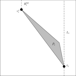
Assume that we are given a cell for which we want to compute the optimal solution. We guess the triangle in the optimal solution to this cell such that is closest to the right edge of the knapsack, and its placement in the optimal solution to . Let such that . We will prove in the next lemma that the optimal solution to consists of and the optimal solutions to two other DP-cells, see Figure 4.
Lemma 27.
Let be a DP-cell, let , and let be two triangles with and let be placements for them. Then there are disjoint sets such that
-
(1)
if , then its optimal solution consists of and the optimal solutions to the cells and ,
-
(2)
if then its optimal solution consists of and the optimal solutions to the cells and ,
-
(3)
if then its optimal solution consists of and the optimal solutions to the cells and ,
-
(4)
if then the optimal solution to consists of and the optimal solutions to the cells and .
Proof.
Let denote the optimal solution to the cell .
Claim.
Consider a feasible solution for the cell . Let be the triangle in whose vertex is closest to the right edge of the knapsack. Then it holds that for each triangle .
Proof of Claim..
If this was not the case then there would be a triangle that intersects . Hence, has one vertex that is closer to the right edge of the knapsack than . In particular, is closer to the right edge of the knapsack than which yields a contradiction. ∎
First assume that . By Lemmas 26 and the Claim no triangle in intersects or and no triangle in has a vertex on the right of . Hence, each triangle in is contained in the area corresponding to the cells and . We define to be the set of indices such that in there is a triangle contained in the area corresponding to and similarly. The other cases can be verified similarly ∎
We guess the sets according to Lemma 27 and store in the solution consisting of , and the solutions stored in the two cells according to the lemma. At the end, the cell (whose corresponding region equals to ) contains the optimal solution.
Lemma 28.
There is an algorithm with a running time of that computes a solution such that .
Proof.
Since we applied Lemma 41 there are only different placements for each triangle. Also, there are only possibilities for the set in the description of the DP-cell. Therefore, the number of DP-cells is bounded by . In order to compute the value of a DP-cell , we guess the triangle and its corresponding placement , and in particular we reject a guess if is not contained in the region corresponding to . Also, we guess and for which there are only possibilities each and reject guesses which do not satisfy that , , and that . Therefore, in each DP-cell we store a solution that is feasible. We can fill the complete DP-table in time . Using Lemma 27 one can show that the cell contains a solution such that with weight at least . ∎
2.4.3. Existence of profitable top-left- or bottom-right-packable solution
In this subsection we prove Lemma 22. Let be a constant to be defined later. Like in the proof of Lemma 19, we observe that there can be only classes containing polygons whose respective values are not larger than ; recall that is the length of the diagonal of . Furthermore, we have that in any placement of inside the angle between the line segment defining (i.e., the line segment connecting the two vertices of with maximum distance) and the bottom edge of the knapsack is essentially . This implies that and are essentially . Finally, recall that as defined in Lemma 16 this is at most . We summarize this in the next proposition.
Proposition 29.
For each there is a constant such that each polygon satisfies that:
-
(1)
,
-
(2)
,
-
(3)
,
-
(4)
,
-
(5)
.
Proof.
We only prove 1 and 5 as 2, 3 and 4 are direct consequence of 1. Note that by choosing we get that:
We now prove that . Let . By part one of this proposition we assume that . Therefore:
Due to Lemma 18 there can be only hard polygons in . Hence, it suffices to prove the claim for the hard polygons in since otherwise the second case of Lemma 22 applies if we define that contains the polygon in of maximum weight. Note that it holds that each triangle intersects the line segment that we define to be the line segment that connects with . Let denote the subsegment of that connects with and let denote the line segment connecting with . Now each triangle in either overlaps or intersects but not or it intersects but not . Therefore, by losing a factor of 3 we can restrict ourselves to one of these cases.
Lemma 30.
If is sufficiently small then by losing a factor 3 we can assume that for each triangle we have that or that .
Proof.
There can be at most one triangle that overlaps . Each other triangle satisfies that or that . If the triangles satisfying have a total weight of at least or if then we are done. Otherwise the triangles satisfying that have a total weight of at least and we establish the claim of the lemma by rotating by 180°. ∎
If then we are done. Therefore, assume now that for each . In the next lemma we prove that by losing a factor of we can assume that the triangles in intersect in the order of their groups (assuming that is a sufficiently small constant). We call such a solution group-respecting as defined below.
Definition.
Let be a solution in which each triangle intersects and assume w.l.o.g. that the triangles in intersect in the order when going from to . We say that is group-respecting if for any two triangles with and for some it holds that .
For each let denote the length of the intersection of and in the placement of .
Lemma 31.
If is sufficiently small, then by losing a factor we can assume that is group-respecting and that for each .
Proof.
Due to Lemma 18 we lose only a factor by requiring that for each . We prove now that by losing another factor we can assume that is group-respecting.
Let . Let be the longest edge of in the placement of in . Let be the angle between and .
Like in the proof of Lemma 16 we define . Intuitively, using we can define two hexagonical areas close to the diagonals of the knapsack such that the longest edge of lies within or within . Also, let denote the length of the line segment . Observe that .
Let denote the rectangle obtained by taking the bounding box of and moving and rotating it such that one of its edges coincides with (in the placement of ) inside . Note that the intersection of and has length at most by Proposition 29. Therefore, . On the other hand, if is sufficiently small then and thus . Also, it holds that and hence . Let be a constant such that for each .
Then there exists a constant such that the following holds. For any two polygons , such that we have that since and for each constant we can guarantee that if we choose sufficiently large. Let be the longest edge of . Assume w.l.o.g. that lies within . However, we have that . Since and do not intersect, they must therefore be placed in a group-respecting manner in .
We split into groups such that for each offset we define . Therefore, for each solution it holds that for any two distint polygons , for values it holds that and are placed in a group-respecting manner in . Then taking the most profitable solution among the solutions loses at most another factor . ∎
For each triangle let be the vertex adjacent to the two longest edges of in the placement of in . Also, let denote the angle at . We note that there exist only constantly many triangles with .
Lemma 32.
There exist at most triangles in such that .
Proof.
Let . Note that the triangle with angle at and side lengths and is contained in (otherwise is not adjacent to the two longest sides). Therefore:
Hence there can only be at most such triangles in . ∎
Due to Lemma 32 we assume now for each . Furthermore, since each triangle is very wide, must be close to one of the four corners of since otherwise the longest edge of does not fit into . Thus, by losing a factor 4 we assume that is close to for each .
Lemma 33.
By losing a factor we can assume for each that
Proof.
Let be the vertices that define . By Claim Claim we know that or is at distance of some corner of . Without loss of generality and applying Proposition 29 we assume that . Recall that by Proposition 29 . Hence:
Let and call the corner furthest away from . Note that , from which we conclude that every endpoint of the diagonal is at distance at most from a corner. In particular must be a distance at most from some corner.
We define and , , in a similar fashion. These sets partition into four sets. Note that one of these sets must have weight at least . If this set is we are done. Otherwise, we simply rotate accordingly. ∎
Due to Lemma 33, if is sufficiently small we have for each triangle that both and intersect the right edge of the knapsack or both and intersect the bottom edge of the knapsack. We call triangles of the former type right-facing triangles and we call the triangles of the latter type bottom-facing triangles.
Proposition 34.
If is sufficiently small, we have that by losing a factor of 2 we can assume that each triangle in is right-facing or bottom-facing.
Assume that . We partition now into groups such that each group is top-left-packable. Then the most profitable such group yields a -approximation. We initialize and . Suppose inductively that for some we partitioned the triangles into such that each of these sets is top-left-packable. We argue that there is one value such that is also top-left-packable. To this end, observe that in the top-left-packing of each set each triangle blocks a certain portion of such that no other triangle in this packing can overlap this part of . To this end, for each triangle let be the smallest integer such that if for some then in the top-left packing of the longest edge of lies on the line that contains and . Also, let be the smallest integer such that and does not overlap the point . Then, after placing we cannot add another triangle in a top-left-packing to that touches the subsegment of that connects with . Hence, intuitively blocks the the latter subsegment. We define . Our crucial insight is now that up to a constant factor, in our top-left packing the triangle blocks as much of as it covers of in .
Lemma 35.
If is sufficiently small then for each triangle it holds that .
Proof.
We argue in a similar way as in the proof of Lemma 31. Let be the longest edge of in an arbitrary placement of inside . Let denote the length of the intersection of and in this placement. Let be the angle between and . Due to Proposition 29 we can assume that . Hence, if is a sufficiently small then the intersection of and has length at most . Therefore, .
On the other hand, if sufficiently small then . Hence, and also and therefore . Since this implies that . Also, it holds that and lies in or . Therefore, if is sufficiently large (which implies that the points are sufficiently dense on ) we have that . ∎
Lemma 35 implies that if is a sufficiently large constant then there is a value such that . Hence, in the top-left packing for (which at this point contains only triangles from ) the triangles block less of than the amount of that the triangles cover in . On the other hand, we know that in the triangle is placed such that it intersects further on the right than any triangle in due to Lemma 31. Using this, in the next lemmas we show that we can add to .
Lemma 36.
If each triangle in is right-facing we have that is top-left-packable.
Proof.
Let and . Consider now and define the point as the intersection between the right side of the Knapsack and . Similarly, define as the intersection between and the line obtained by rotating around by counterclockwise. Note that every polygon in is contained in as they are top-left-packed.
We translate upwards until it intersects the top side of the knapsack at a point . By Lemma 33 we get that . Note that now is placed inside the triangle . Define now , . Note that it suffices to prove that and for each as this implies that can be placed inside the triangle with vertices , this triangle is contained in and this placement is group respecting.
Since and , a similarity argument between triangles and lets us obtain:
| (1) |
As we obtain , implying that and therefore we only need to prove that for each . Pythagoras theorem on gives us:
| (2) |
We now compute .
Note that if and only if . After some algebra we obtain the following:
We can compute the discriminant of this polynomial and obtain:
since (as intersects by at least and the amount intersects ). Therefore has a unique real root . Note that . We begin by showing that . Indeed:
Therefore . If , then it is clear that . Suppose then that . Since:
then for by continuity. Therefore is decreasing in concluding that and that for .
Let be the angle between and . Let be the placement of the vertex of that is not adjacent to the longest edge. We aim to show that implying that is placed inside the Knapsack. By examining the triangle , , we get that .
Furthermore by applying the law of sines on triangle , , we get:
Therefore . By choosing small enugh we assume that . Note that by choosing small enough . Therefore:
Which implies that or . If then which is not possible. We conclude that and since we conclude that . It only remains to prove that the same holds for .
Let be the vertex of that is not or . Let be the angle of at and the angle between and . Note that , therefore . By examining the triangle , , we obtain that . Therefore:
We conclude that for each other . Call and the rotation matrix by , then: .
In particular , from which we conclude. ∎
Lemma 37.
If each triangle in is bottom-facing we have that is bottom-right-packable.
Proof.
Let , and . We define as . Define as the intersection between and the bottom edge of . Similarly, let be the rotation of by counterclockwise and call the intersection between and the bottom edge. Let also the triangle , , . We begin by rotating by 180° around .
We now translate upwards until it intersects the top-edge of the Knapsack at for some . Note that is contained inside the triangle
Let be the amount intersects . A similarity argument between and , , gives us:
Since we obtain .
We now translate to the left until coincides with . Let be the rightmost point in . Since we know that . Therefore is placed to the left of the line that passes through and . Furthermore, is to the right of as they are bottom-right packed. We know rotate counterclockwise around until it overlaps . Finally, by rotating 180° around we arrive at a bottom-right packing of . ∎
We add to . We continue iteratively until we assigned all triangles in to the sets . Then the most profitable set among them satisfies that . On the other hand, . Hence, or which completes the proof of Lemma 22.
2.5. Hard polygons under resource augmentation
Let . We consider the setting of -resource augmentation, i.e., we want to compute a solution that is feasible for a knapsack of size and such that where is the optimal solution for the original knapsack of size . Note that increasing by a factor of is equivalent to shrinking the input polygons by a factor of .
Given a polygon defined via coordinates we define to be the polygon with coordinates where and for each . For each input polygon we define its shrunk counterpart to be . Based on we define sets and the set for each in the same way as we defined and based on above.
For the sets and we use the algorithms due to Lemmas 6 and 7 as before. For the hard polygons we can show that there are only groups that are non-empty, using that we obtained them via shrinking the original input polygons. Intuitively, this is true since for each where denotes the length of the longest diagonal of , and hence if .
Lemma 38.
We have that if . Hence, there are only values such that .
Proof.
Let be an arbitrary polygon. Note that , and therefore . We conclude that . Note that, for any , if is non-empty, there must be a that satisfies (or equivalently ). We conclude that such ’s must verify and therefore there are at most non-empty ∎
Lemmas 18 and 38 imply that where denotes the optimal solution for the polygons in . Let denote the set due to Lemma 19 when assuming that are the hard polygons in the given instance. Therefore, we guess in time . Finally, we output the solution of largest weight among and the solutions due applying to Lemmas 6 and 7 to the input sets and , respectively. This yields the proof of Theorem 3.
3. Optimal profit under resource augmentation
In this section we also study the setting of -resource augmentation, i.e., we want to compute a solution which is feasible for an enlarged knapsack of size , for any constant . We present an algorithm with a running time of that computes such a solution with where is the optimal solution for the original knapsack of size . In particular, we here do not lose any factor in our approximation guarantee.
First, we prove a set of properties that we can assume “by -resource augmentation” meaning that if we increase the size of by a factor then there exists a solution of weight with the mentioned properties, or that we can modify the input in time such that it has these properties and there still exists a solution of weight .
3.1. Few types of items
We want to establish that the input polygons have only different shapes. Like in Section 2 for each polygon denote by its bounding box with width and height . Note that . The bounding boxes of all polygons such that have a total height of at most . Therefore, we can pack all these polygons into the extra capacity that we gain by increasing the size of by a factor and therefore ignore them in the sequel.
Lemma 39.
By -resource augmentation we can assume for each that and that .
Proof.
Let be the two vertices that define . Note that by the triangle inequality and by definition, concluding that . Additionally, let be the polygons that satisfy . Note that , and therefore, we can pack these polygons into the extra capacity. Finally, by Lemma 10 for each remaining polygon . ∎
Next, intuitively we stretch the optimal solution by a factor which yields a container for each polygon which contains and which is slightly bigger than . We define a polygon such that and that globally there are only different ways can look like, up to translations and rotations. We refer to those as a set of shapes of input objects. Hence, due to the resource augmentation we can replace each input polygon by one of the shapes in .
Lemma 40.
By -resource augmentation we can assume that there is a set of shapes with such that for each there is a shape such that and has only many vertices.
Proof.
Let be an input polygon. Assume that is rotated such that its longest diagonal is horizontal, i.e., let denote the vertices of with largest distance; we assume that and lie on a horizontal line, i.e., that . Furthermore, let denote the vertices of with minimum and maximum -coordinate, respectively (see Figure 6).
Note that extending the knapsack by a factor is equivalent to shrinking each input polygon by a factor . Let denote the polygon obtained by shrinking towards the origin, i.e., by replacing each vertex of by the vertex . Our goal is to show that there exists a polygon whose shape is one shape out of options such that there is a translation vector with . Then we replace in the input the polygon by a polygon which is congruent to . Hence, for the shapes of the resulting polygons there are only options. In the process, we will shrink a constant number of times. Then the claim follows by redefining accordingly.
First, we shrink by a factor of at most such that the line segment connecting and has a length that is a power of . Let denote this new length. Since originally there are only options for . We partition the bounding box of into four rectangles where
-
•
is the (unique) rectangle with vertices and ,
-
•
is the (unique) rectangle with vertices and ,
-
•
is the (unique) rectangle with vertices and , and
-
•
is the (unique) rectangle with vertices and .
We translate such that is the origin. If the width of is smaller than then intuitively we shrink by a factor towards such that is again a power of and . More formally, we replace each vertex of by a vertex such that and for some value . First, we move towards such that is the next smaller power of . Then we move towards such that . Finally, we move each remaining vertex by exactly a factor towards . As a result, becomes empty. We perform similar operations in case that the width of , or is smaller than . Also, we perform a similar operation in case that the height of (identical to the height of ) is smaller than or that the height of (identical to the height of ) is smaller than . In the latter operations we move the vertices of towards or , respectively.
Assume again that is the origin. Let . Let such that , and is the smallest value with such that the distance between and is a multiple of . In particular, then and note that is the width of for which holds.
We define such that and is that largest value such that lies inside . Observe that since includes all points on the line segment connecting and by convexity. Similarly, we define a point between and and a corresponding point . We move each vertex of towards that satisfy that and , i.e., we reduce the distance between and by a factor which we justify via shrinking. One can show that afterwards lies in the convex hull spanned by the other vertices of and and , using that . Hence, we can remove .
We move such that becomes the origin. Let denote the (unique) rectangle with vertices and . Our goal is now to move the vertices within such that only vertices remain and that for the coordinate of each of them there are only options. Whenever we move a vertex within we move towards such that the distance between and decreases by at most a factor but keep and unchanged. In this way the distance between and does not change and the distance between and does not change either. Let denote the distance between and and let denote the distance between and . Assume w.l.o.g. that and that is the origin. Observe that by convexity each point on the line segment connecting and lies within .
Let be a constant with to be defined later. We shoot rays originating at such that goes through , goes through , and between any two consecutive rays there is an angle of exactly (see Figure 7).
For each denote by the point on the boundary of that is intersected by (not necessarily a vertex of ). Imagine that we shrink such that we move each vertex of towards , i.e., we replace by the point . We argue that lies in the convex hull of and hence we can remove . Let be a ray originating at and going through . Suppose that and are the rays closest to . Let and . Then lies in the convex hull of and the point . We have that and or that and . Assume w.l.o.g. that and . We claim that then . The first two inequalities follow from convexity. For proving that , we can assume that since otherwise the claim is immediate. This implies that . Also observe that since otherwise would not be on the boundary of , by convexity. Therefore, cannot be larger than the -coordinate of the point on with -coordinate . Using that one can show that there is a choice for that ensures that . Finally, for each point with we move towards such that the distance between and becomes a power of . Since before the shrinking this distance there are only options for the resulting distance.
In a similar way we define , and and perform a symmetric operation on them. The resulting polygon is defined via , the positions of , the positions of the vertices and (which are defined analogously to and ), for the distance between and and the distances of the vertices to , and the respective values for , and . For each of these values there are only options and there are such values in total. Hence, there are possibilities for the resulting shape. ∎
Finally, we ensure that for each polygon we can restrict ourselves to only possible placements in .
Lemma 41.
By -resource augmentation, for each polygon we can compute a set of at most possible placements for in time such that if then in the polygon is placed inside according to one placement .
Proof.
First, we prove that for each polygon it suffices to allow only possible vectors when defining its placement as . To this end, assume that . For each polygon denote by its corresponding placement in . We assume that for any with it holds that intuitively lies on the left of . Formally, we require that if there is a horizontal line that has non-empty intersection with both and then lies on the left of . Since the polygons are convex such an ordering exists.
Now for each we move by units to the right. Since the resulting placement fits into the knapsack using -resource augmentation. Intuitively, in the resulting placement, each polygon has units of empty space on its left and on its right.
In a similar fashion we move all polygons up such that they still fit into the knapsack under -resource augmentation and intuitively, each polygon has units of empty space above and below it. For each polygon let be its first vertex . We move each polygon such that is placed on a point whose coordinates are integral multiples of . For achieving this, it suffices to move by at most units down and by at most units to the left. By the above, we can do this for all polygons simultaneously without making them intersect. Also, intuitively each polygon still has units of empty space around it in all four directions.
Now we argue that we can rotate each polygon such that its angle is one out of many possible angles. Consider a polygon . Suppose that we rotate it around its vertex . We want to argue that if we rotate by an angle of at most then this moves each vertex of by at most units. Let be a vertex of with . Let denote the distance between the old and the new position of if we rotate by an angle of . Then we have that , assuming that and that is sufficiently small.
Therefore, we rotate around by an angle of at most such that for an angle which is an integral multiple of . Due to our movement of before we can assume that satisfies that and are integral multiples of . Thus, for and for there are only possibilities which yields only possible placements for . ∎
3.2. Recursive algorithm
We describe our main algorithm. First, we guess how many polygons of each of the shapes in are contained in . Since there are only different shapes in we can do this in time . Once we know how many polygons of each shape we need to select, it is clear which polygons we should take since if for some shape we need to select polygons with that shape then it is optimal to select the polygons in of shape with largest weight. Therefore, in the sequel assume that we are given a set of polygons and we want to find a packing for them inside .
Our algorithm is recursive and it generalizes a similar algorithm for the special case of axis-parallel rectangles in [AW14]. On a high level, we guess a partition of given by a separator which is a polygon inside . It has the property that at most of the polygons of lie inside and at most of the polygons of lie outside . We guess how many polygons of each shape are placed inside and outside in . Then we recurse separately inside and outside . For our partition, we are looking for a polygon according to the following definition.
Definition.
Let and . Let be a set of pairwise non-overlapping polygons in . A polygon is a balanced -cheap -cut if
-
•
has at most edges,
-
•
the polygons contained in have a total area of at most ,
-
•
the polygons contained in the complement of , i.e., in , have a total area of at most , and
-
•
the polygons intersecting the boundary of have a total area of at most .
In order to restrict the set of balanced cheap cuts to consider, we will allow only polygons such that each of its vertices is contained in a set of size defined as follows. We fix a triangulation for each placement of each polygon . We define a set where for each placement for we add to the positions of the vertices of . Also, we add the four corners of to . Let denote the set of vertical lines such that is the -coordinate of one point in . We define a set where for each placement of each , each edge of a triangle in the triangulation of , and each vertical line we add to the intersection of and . Also, we add to the intersection of each line in with the two boundary edges of . Let denote the set of all intersections of pairs of line segments whose respective endpoints are in . We define . A result in [AW14] implies that there exists a balanced cheap cut whose vertices are all contained in .
Lemma 42 ([AW14]).
Let and let be a set of pairwise non-intersecting polygons in the plane with at most edges each such that for each . Then there exists a balanced -cheap -cut whose vertices are contained in .
Our algorithm is recursive and places polygons from , trying to maximize the total area of the placed polygons. In each recursive call we are given an area and a set of polygons . In the main call these parameters are and . If then we return an empty solution. If there is a polygon with then we guess a placement and we recurse on the area and on the set . Otherwise, we guess the balanced cheap cut due to Lemma 42 with and for each shape we guess how many polygons of with shape are contained in , how many are contained in , and how many cross the boundary of (i.e., have non-empty intersection with the boundary of ). Note that there are only possibilities to enumerate. Let , and denote the respective sets of polygons. Then we recurse on the area with input polygons and on the area with input polygons . Suppose that the recursive calls return two sets of polygons and that the algorithm managed to place inside the respective areas and . Then we return the set for the guesses of , , and that maximize . If we guess the (correct) balanced cheap cut due to Lemma 42 in each iteration then our recursion depth is since the cuts are balanced and each polygon has an area of at least (see Lemma 39). Therefore, if in a recursive call of the algorithm the recursion depth is larger than then we return the empty set and do not recurse further. Also, if we guess the correct cut in each node of the recursion tree then we cut polygons whose total area is at most a -fraction of the area of all remaining polygons. Since our recursion depth is , our algorithm outputs a packing for a set of polygons in with area at least . This implies the following lemma.
Lemma 43.
Assume that there is a non-overlapping packing for in . There is an algorithm with a running time of that computes a placement of a set of polygons inside such that .
It remains to pack the polygons in . The total area of their bounding boxes is bounded by . Therefore, we can pack them into additional space that we gain via increasing the size of by a factor , using the Next-Fit-Decreasing-Height algorithm [CGJT80].
Theorem 44.
There is an algorithm with a running time of that computes a set with such that fits into under -resource augmentation.
References
- [AW14] Anna Adamaszek and Andreas Wiese. A QPTAS for maximum weight independent set of polygons with polylogarithmically many vertices. In Proceedings of the 25th Annual ACM-SIAM Symposium on Discrete Algorithms (SODA 2014), pages 645–656. SIAM, 2014.
- [AW15] Anna Adamaszek and Andreas Wiese. A quasi-PTAS for the two-dimensional geometric knapsack problem. In Proceedings of the 26th Annual ACM-SIAM Symposium on Discrete Algorithms (SODA 2015), pages 1491–1505. SIAM, 2015.
- [BCJ+09] Nikhil Bansal, Alberto Caprara, Klaus Jansen, Lars Prädel, and Maxim Sviridenko. A structural lemma in 2-dimensional packing, and its implications on approximability. In Algorithms and Computation (ISAAC 2009), volume 5878 of LNCS, pages 77–86. Springer, 2009.
- [CGJT80] Edward G Coffman, Jr, Michael R Garey, David S Johnson, and Robert Endre Tarjan. Performance bounds for level-oriented two-dimensional packing algorithms. SIAM Journal on Computing, 9:808–826, 1980.
- [CK00] Chandra Chekuri and Sanjeev Khanna. A ptas for the multiple knapsack problem. In Proceedings of the Eleventh Annual ACM-SIAM Symposium on Discrete Algorithms, SODA ’00, pages 213–222, USA, 2000. Society for Industrial and Applied Mathematics.
- [GGH+17] Waldo Gálvez, Fabrizio Grandoni, Sandy Heydrich, Salvatore Ingala, Arindam Khan, and Andreas Wiese. Approximating geometric knapsack via l-packings. In 58th IEEE Annual Symposium on Foundations of Computer Science, FOCS 2017, Berkeley, CA, USA, October 15-17, 2017, pages 260–271, 2017.
- [HW19] Sandy Heydrich and Andreas Wiese. Faster approximation schemes for the two-dimensional knapsack problem. ACM Trans. Algorithms, 15(4):47:1–47:28, 2019.
- [Jin19] Ce Jin. An improved FPTAS for 0-1 knapsack. In 46th International Colloquium on Automata, Languages, and Programming, ICALP 2019, July 9-12, 2019, Patras, Greece, pages 76:1–76:14, 2019.
- [JSO07] Klaus Jansen and Roberto Solis-Oba. New approximability results for 2-dimensional packing problems. In Mathematical Foundations of Computer Science (MFCS 2007), volume 4708 of LNCS, pages 103–114. Springer, 2007.
- [JSO08] Klaus Jansen and Roberto Solis-Oba. A polynomial time approximation scheme for the square packing problem. In Integer Programming and Combinatorial Optimization (IPCO 2008), volume 5035 of LNCS, pages 184–198. Springer, 2008.
- [JZ04a] Klaus Jansen and Guochuan Zhang. Maximizing the number of packed rectangles. In Algorithm Theory (SWAT 2004), volume 3111 of LNCS, pages 362–371. Springer, 2004.
- [JZ04b] Klaus Jansen and Guochuan Zhang. On rectangle packing: maximizing benefits. In Proceedings of the 15th Annual ACM-SIAM Symposium on Discrete Algorithms (SODA 2004), pages 204–213. SIAM, 2004.
- [LMX18] Carla Negri Lintzmayer, Flávio Keidi Miyazawa, and Eduardo Candido Xavier. Two-dimensional knapsack for circles. In Latin American Symposium on Theoretical Informatics, pages 741–754. Springer, 2018.
- [LTW+90] Joseph YT Leung, Tommy W Tam, CS Wong, Gilbert H Young, and Francis YL Chin. Packing squares into a square. Journal of Parallel and Distributed Computing, 10(3):271–275, 1990.
- [Ste97] A Steinberg. A strip-packing algorithm with absolute performance bound 2. SIAM Journal on Computing, 26(2):401–409, 1997.