Sensitivity of the Cherenkov Telescope Array to a dark matter signal from the Galactic centre

Abstract

We provide an updated assessment of the power of the Cherenkov Telescope Array (CTA) to search for thermally produced dark matter at the TeV scale, via the associated gamma-ray signal from pair-annihilating dark matter particles in the region around the Galactic centre. We find that CTA will open a new window of discovery potential, significantly extending the range of robustly testable models given a standard cuspy profile of the dark matter density distribution. Importantly, even for a cored profile, the projected sensitivity of CTA will be sufficient to probe various well-motivated models of thermally produced dark matter at the TeV scale. This is due to CTA’s unprecedented sensitivity, angular and energy resolutions, and the planned observational strategy. The survey of the inner Galaxy will cover a much larger region than corresponding previous observational campaigns with imaging atmospheric Cherenkov telescopes. CTA will map with unprecedented precision the large-scale diffuse emission in high-energy gamma rays, constituting a background for dark matter searches for which we adopt state-of-the-art models based on current data. Throughout our analysis, we use up-to-date event reconstruction Monte Carlo tools developed by the CTA consortium, and pay special attention to quantifying the level of instrumental systematic uncertainties, as well as background template systematic errors, required to probe thermally produced dark matter at these energies.

1 Introduction

There is compelling evidence that a cold, non-baryonic dark matter (DM) component dominates the matter content of the Universe at cosmological scales, contributing a fraction of about 27% to its total energy density [1]. The underlying nature of this DM component is still unknown, a century after its existence was first conjectured [2], but many hypothetical elementary particles may provide viable solutions [3, 4, 5]. In particular, even if increasingly pressured by lack of experimental evidence [6], weakly interacting massive particles (WIMPs) remain one of the best-motivated candidates [7]. Such particles with masses and couplings at the electroweak scale would be a compelling solution to the DM puzzle not only because their existence could point to a way of addressing the naturalness problems in the standard model of particle physics (SM), but also because it would allow us to understand the presently measured DM abundance as a result of the standard thermal history of the Universe [8].

Searches for signals of DM annihilation in astrophysical objects are sensitive to the same physical process as the one that, in these models, took place in the early Universe. In fact, the WIMP paradigm makes a clear prediction for the annihilation cross-section of interest, and hence the expected signal strength. Among the various possible ways of detecting such indirect detection signals, gamma rays are particularly promising (for a review, see Ref. [9]). By far, the largest signal is expected from the region around the Galactic centre (GC), which is both one of the closest DM targets and features the highest DM density in our Galaxy [10].

The Cherenkov Telescope Array (CTA) [11] is now close to entering the production phase and will be the world’s most sensitive gamma-ray telescope for a window of photon energies stretching more than three orders of magnitude, from a few tens of GeV to above 300 TeV, with an angular resolution that is better than any existing instrument observing at frequencies higher than the X-ray band. One of CTA’s main science drivers is the search for a signal from annihilating DM [12]. Previous estimates indicate that CTA observations of the GC have a good chance of being sensitive to the ‘thermal’ annihilation cross section [13, 14, 15, 16, 17, 18], i.e. the WIMP annihilation strength required to explain the observed DM abundance in the simplest models from particle physics. For TeV-scale DM, notably, CTA might well turn out to be the only planned or existing instrument with this property (another potential contender being AMS-02 [19] via charged cosmic rays, CRs [20, 21]); it thus provides an important tool to search for WIMPs that is highly complementary to direct DM searches in underground laboratories or WIMP searches at colliders [22, 23, 24, 25].

Given the imminent start of the telescope construction, and the strong science case outlined above, it is timely to move beyond existing analyses and provide more realistic sensitivity estimates to a DM signal from GC observations with CTA that fully take into account the current best estimates for the expected telescope characteristics as well as recent developments in understanding the (expected) Galactic diffuse emission (GDE) components in that region. In fact, CTA is expected to measure some of the GDE components with an unprecedented angular resolution at TeV energies – which is a prominent science goal in itself. Here we report on such an updated analysis and explore the most promising strategies to define signal regions and data analysis methods, using state-of-the-art models for astrophysical and instrumental backgrounds. In particular, a major motivation of this work is to study in detail the applicability of a full template fitting approach in the analysis of imaging atmospheric Cherenkov telescopes (IACT) data, a field which has traditionally mostly relied on separate ‘ON’ and ‘OFF’ regions to extract the DM signal and background, respectively (though first studies indicate the advantages of moving beyond that method [14]).

We present our results for standard assumptions concerning the DM density profile, both in terms of expected sensitivities to the annihilation cross-section for the most commonly adopted annihilation channels and in the form of tabulated likelihoods that can be applied to almost arbitrary annihilation spectra, and we discuss in detail how these assumptions affect our conclusions. We further demonstrate that the DM sensitivity is, indeed, quite significantly affected by the expected GDE, which makes realistic modelling of this component mandatory. As expected for an instrument with a large collection area and excellent event statistics such as CTA [9], finally, we confirm that the sensitivity is, in large parts of the parameter space, limited by systematic rather than statistical uncertainties. We, therefore, put special emphasis on discussing this aspect, both regarding the overall uncertainty and bin-to-bin correlations in sky positions and energy. This allows us to quantify the maximal level of systematic uncertainty that is required to reach the thermal cross-section for a given DM mass and annihilation channel (assuming a standard DM density profile).

This article treats a range of topics, from DM to conventional astrophysics and instrumental properties. While we make an effort to cover all relevant aspects, which makes a certain overall length unavoidable, we deliberately organised the article in a way that allows the reader to directly skip to the (mostly self-contained) sections of interest without the need to read all preceding parts. We start by briefly introducing high-energy gamma-ray astronomy and the CTA observatory in Section 2, along with its planned observational strategy for the GC region. We then describe in more detail the expected DM signal and various astrophysical and instrumental background sources in the GC region (in Section 3), as well as the data analysis techniques adopted in our analysis (in Section 4). We present our findings concerning the projected sensitivity of CTA to a DM signal in Section 5; as this is a concise summary of our main results, many readers would typically directly want to jump there. In Section 6 we discuss in more detail how these results depend on the adopted analysis strategy and the treatment of the astrophysical emission components, before concluding in Section 7. In an extended appendix, we collect supplemental material to further support the discussion section, as well as more technical background information about the analysis pipeline. In Appendix A, in particular, we show projected sensitivities for the reduced telescope configuration that will be implemented in the initial construction phase.

2 Gamma-ray astronomy and CTA

2.1 Telescope design and historical context

From a historic point of view, gamma-ray astronomy started with satellite-based studies of high energy ($>50$ MeV) photon emission. In particular, the OSO-3 satellite [26], launched in 1967, was the first to detect the Galactic centre and Galactic plane [27], as well as the presence of an isotropic extragalactic gamma-ray background [28]. In the following decades, satellite missions like SAS-2 (1972) [29], COS-B (1975) [30], EGRET (1991) [31] and the most recent representatives AGILE [32] and Fermi-LAT [33] have widely increased our knowledge of the gamma-ray sky. Nonetheless, due to their limited size, satellites can typically only cover energies below the TeV range.

The very high-energy sky can be observed with ground-based gamma-ray telescopes. This approach was pioneered by the Whipple telescope [34] in the late 1980s, demonstrating the promise of the imaging atmospheric Cherenkov light technique which rests on imaging short flashes of Cherenkov radiation produced by cascades of relativistic charged particles in the atmosphere, originating from very high energy gamma rays or charged cosmic rays striking the top of the atmosphere (see, e.g., Ref. [35] and references therein). The technique was further developed with the current set of modern IACTs, demonstrating a leap in sensitivity by increasing the telescope multiplicity [43, 44]. In comparison, day-long observations at sub-TeV energies with modern IACTs like H.E.S.S. [45], MAGIC [46] and VERITAS [47] very roughly result in similar sensitivities as year-long satellite observations. IACTs have mapped the very high energy gamma-ray sky, resulting in a catalogue of about two hundred TeV sources [48], including active galactic nuclei (AGNs) as the most numerous extragalactic source class and tens of Galactic sources, most importantly supernova remnants (SNRs) and pulsar wind nebulae (PWNe). IACT data was also used to set competitive limits on the annihilation of TeV-scale DM candidates, falling just short of reaching the theoretically motivated ‘thermal’ cross-section value (see e.g. [49, 50, 51, 52]).

CTA is the next-generation IACT gamma-ray observatory [12, 11]. When completed it will comprise two arrays, a southern one being located at the European Southern Observatory (ESO) site in Chile, Atacama desert, and a northern one being located at the Roque de los Muchachos Observatory (ORM) site in La Palma, Canary Islands. This combination will make CTA the first ground-based gamma-ray telescope with the capability to observe a large sky fraction. The CTA design concept foresees three types of telescopes with different sizes: i) LSTs (Large-Sized Telescopes, 23 m in diameter) that are needed to detect the relatively small amount of Cherenkov photons from gamma rays in the 20 – 150 GeV range, ii) MSTs (Medium-Sized Telescopes, 11.5 m) that aim to observe energies between 150 GeV and around 5 TeV, and iii) a large number of SSTs (Small-Sized Telescope, 4 m), spread out over several square kilometers to detect the most energetic, but very rare gamma rays. The ‘baseline’ goal, which we base our sensitivity forecast on, is to deploy 4 LSTs at each of the sites, 25 (15) MSTs in the Southern (Northern) hemisphere, and 70 SSTs at the southern site (see Appendix A for the effects of a slimmed-down, initial configuration). As a result of this setup, CTA is believed to be large and sensitive enough to bridge the characteristic differences between current IACTs and satellite-borne gamma-ray telescopes, spanning a range of observable energies from 10s of GeV up to above 300 TeV. The large field of view cameras will also put CTA in a unique position to perform surveys of extended sky regions. Those currently planned include the GC survey and extended GC survey described in Section 2.2, but also an extensive survey of the Galactic plane as well as an extragalactic survey covering a quarter of the Northern sky [12].

2.2 Observational strategy of the Galactic centre

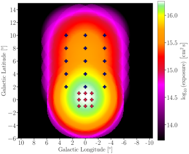
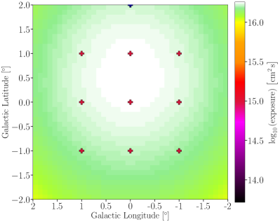
Figure 1: The left panel shows the exposure map for CTA’s Galactic centre (GC) and extended GC surveys, at an energy of 1 TeV. The right panel shows a zoom into the GC survey region. The nine pointing positions of the GC survey mode are marked with red crosses. The observation time for each of these pointing positions will be approximately $60\,\textrm{h}$. The 15 pointing positions of the extended survey north of the Galactic plane are marked with blue crosses. The observation time for each position will be $20\,\textrm{h}$ in this case.

Given its importance for both DM and astrophysical studies, a significant fraction of the currently planned CTA observing time for key science projects is dedicated to a detailed exploration of the GC region [12]. Surveys of extended portions of the sky will be adopted as an observational strategy that, in scope and ambition, will surpass previous gamma-ray observations with IACTs. Below we detail surveys which (in part) overlap with the Galactic center region:

• Galactic centre Survey: This is the survey strategy that CTA will follow according to current plans. It consists of nine individual pointing positions centred on ($l=\pm 1^{\circ},0^{\circ}$, $b=\pm 1^{\circ},0^{\circ}$) in Galactic coordinates (red crosses in Fig. 1), and we evenly distribute the total observation time of $t_{\rm{obs}}=525\;\textrm{h}$ among them. We stress that all three telescope types are part of this observation mode – but with varying actual sensitivity within the field of view (FoV), which is implicitly accounted for through the instrument response functions (IRFs). This is the default pointing strategy as well as the default survey ‘region of interest’ (ROI) we adopt in this article.

• Extended survey: An observation supplementing the GC survey is to scan over a region above the Galactic plane from $b=2^{\circ}$ to $b=10^{\circ}$, and $l=-3^{\circ}$ to $l=+3^{\circ}$, with 15 additional pointing positions centred on ($l=\pm 3^{\circ},0^{\circ}$, $b=2^{\circ},4^{\circ},6^{\circ},8^{\circ},10^{\circ}$) in Galactic coordinates (blue crosses in Fig. 1). Each of those pointing directions is observed for $20\,\textrm{h}$ so that the total observation time of the extended survey amounts to $t_{\rm{obs}}=300\,\textrm{h}$ (adding to the combined 525 h of the GC survey). Due to the large region covered, this observation strategy can increase the sensitivity for DM distributions that are more cored around the GC (as discussed in more detail in Section 5.3).

The planned Galactic plane survey will also overlap with the GC region. However, since it has a significantly smaller exposure than the two surveys described above, we will not use it in our work. To evaluate the expected number of events for a given sky model, the CTA consortium has produced IRFs for the planned array configurations. These are based on Monte-Carlo simulations of the Cherenkov light that is generated in the interaction of gamma rays with the Earth’s atmosphere and the subsequent measurement of this light by CTA telescopes, followed by event reconstruction and classification. The IRFs provide information on effective area, point spread function and energy dispersion as a function of energy and offset angle for various telescope pointing zenith angles [53]. In this work, we use the publicly available prod3b-v1 IRF library, and in particular the IRF file South_z20_average_50h which is optimised – by defining background reduction cuts with respect to an equivalent of 50 h of simulated Monte Carlo air showers – for the detection of a point-like source at $20^{\circ}$ zenith angle (note that the GC is mostly visible from the southern site). Finally, for the smaller number of telescopes planned for the initial construction configuration investigated in Appendix A, we use a separate set of IRFs as described there. A versatile tool to predict the number of expected counts, given a set of IRFs, is the public code ctools [54] that we will make extensive use of in our analysis.

3 Emission components for Galactic centre observations

Here we discuss the various emission components that may appear in the ROI around the GC, starting with the DM contribution and then moving on to the expected conventional astrophysical emission and the contribution from misidentified CRs. We conclude with an explicit comparison of the emission templates that we use (for a quick overview, see Figs. 3 and 4).

3.1 Dark matter contribution

As already stressed in the introduction, CTA provides unique opportunities to test the WIMP paradigm at the TeV scale. Heavy DM candidates falling into this mass range include the (still) most popular lightest neutralino [3], but also candidates appearing in models with extra dimensions [55, 56], or models involving ‘portals’ between the standard model and a dark sector [57, 58, 59, 60], just to name a few. The spectral distribution of the expected gamma rays contains valuable information about the underlying theory. It ranges from relatively soft and featureless spectra to, as in the case of Kaluza-Klein DM [61], rather hard spectra with an abrupt cut-off at energies corresponding to the DM mass; sometimes also pronounced spectral endpoint features are present [62], which have been worked out to high accuracy for theoretically well-motivated candidates like the Wino [63, 64, 65, 66] and Higgsino [67, 68, 69, 18]. Further aspects making the TeV scale particularly interesting from a theoretical perspective include the large flux enhancements that are possible due to the Sommerfeld effect [70] and the fact that this scale is close to the unitarity limit for thermally produced DM [71, 72].

In general, the prompt emission component of the differential gamma-ray flux, per unit energy and solid angle, that is expected from annihilating DM particles $\chi$ with a density profile $\rho_{\chi}(\mathbf{r})$ is given by (see e.g. Ref. [9])

$$\frac{d\Phi_{\gamma}}{d\Omega\,dE_{\gamma}}(E_{\gamma},\psi)=\frac{1}{4\pi}\int_{\mathrm{l.o.s}}d\ell(\psi)\rho_{\chi}^{2}(\mathbf{r})\left({\frac{\langle\sigma v\rangle_{\mathrm{ann}}}{2S_{\chi}m_{\chi}^{2}}\sum_{f}B_{f}\frac{dN_{\gamma}^{f}}{dE_{\gamma}}}\right)\,,$$ (3.1)

where the integration is performed along the line of sight (l.o.s.) in the observing direction ($\psi$). Particle physics parameters that enter here – contained in the parenthesis – are the average velocity-weighted annihilation cross-section $\langle\sigma v\rangle_{\mathrm{ann}}$, the DM mass $m_{\chi}$, a symmetry factor that is $S_{\chi}=1$ ($S_{\chi}=2$) if the DM particle is (not) its own antiparticle, the annihilation branching ratio $B_{f}$ into channel $f$ and the number $N_{\gamma}^{f}$ of photons per annihilation. If the annihilation rate (and spectrum) is sufficiently independent of the small Galactic DM velocities $v(\mathbf{r})$, as for the simplest DM models, the factor in parenthesis can be pulled outside the line-of-sight and angular integrals. Spatial and spectral information contained in the signal then factorise, and hence are uncorrelated, such that the flux from a given angular region $\Delta\Omega$ becomes simply proportional to what is conventionally defined as the ‘$J$-factor’,

$$J\equiv\int_{\Delta\Omega}d\Omega\int\!\!d\ell\,\rho_{\chi}^{2}\,.$$ (3.2)

For simplicity, and in order to make our limits directly comparable to corresponding limits in the literature, we will in the following assume that all of the astrophysically observed DM consists of a single type of self-conjugate particles $\chi$ (i.e. $S_{\chi}=1$); if only a fraction $f_{\chi}$ of the total DM component annihilates, all reported limits weaken by a factor of $f_{\chi}^{2}$.

Spatial distribution

Calculating the $J$-factor to sufficient precision requires a good knowledge of the DM distribution. The average local DM density at the Sun’s distance from the GC, which we take as the canonical $r_{\odot}=8.5\;\textrm{kpc}$ (though recent precision measurements rather indicate a value closer to $r_{\odot}=8.2\;\textrm{kpc}$ [79, 80]), can be determined relatively well by observations. Here we follow the common practice of using $\rho_{\odot}=0.4$ GeV/cm³, noting that the uncertainty associated with this value is typically quoted to be a factor of less than about 2 [81, 82, 83, 84]. The DM content in the inner kpc of the Milky Way (MW), in contrast, is almost unconstrained observationally because the baryonic component largely dominates the gravitational potential in that region [85, 86, 83, 84] (for an early discussion, see also Ref. [87]).

Numerical $N$-body simulations of collision-less cold DM clustering – not including baryonic feedback – have consistently demonstrated, on the other hand, that DM halos should develop a universal density profile during cosmological structure formation, following the gravitational collapse of initially small density perturbations [88, 89, 90]. Largely independent of the virial mass, in particular, such WIMP DM halos today should be ‘cuspy’, with the logarithmic slope at small galactocentric distances $r$ being roughly $d(\log\rho)/d(\log r)\approx-1$. Recent simulations rather tend to favour an Einasto profile [91],

$$\rho_{{\rm Einasto}}\!\left(r\right)=\rho_{s}\exp\!\left(-\frac{2}{\alpha}\left[\left(\frac{r}{r_{s}}\right)^{\alpha}-1\right]\right){\rm,}$$ (3.3)

which is slightly shallower in the central-most parts of the halo than the form originally suggested by Navarro, Frenk and White (NFW) [88, 89]. In our analysis we will adopt benchmark values of $\alpha=0.17$ and $r_{s}=20$ kpc (and hence $\rho_{s}=0.081$ GeV/cm³). This is both compatible with the most recent observations [92] and inside the expected range of these parameters for simulated halos with the mass of the MW [93].

More realistic simulations of MW-like halos necessarily have to include a baryonic component. Baryons can radiate away energy and angular momentum, leading to the formation of disks and much more concentrated densities in the central halo region. The correspondingly larger gravitational potential will then also affect the DM component, leading to a significant steepening of the DM profile (and hence an increase of the $J$-factor) if this process happens adiabatically  [94, 95, 96]. On the other hand, feedback from star formation and supernovae, in particular if happening on short time-scales and hence not adiabatically, leads to the formation of central cores of roughly constant density in the DM profile [97]. The current state of the art in simulations suggests that the latter mechanism can often be decisive in smaller galaxies (with masses $\lesssim 10^{12}\,M_{\odot}$), while in larger galaxies (like the MW, or more massive), the former effect often dominates – i.e. baryons tend to contract rather than dilute the central DM distribution (for a recent discussion specifically applying to the MW, using Gaia DR2 data, see Ref. [98]). Even though there has been significant progress in including baryonic effects in hydrodynamical simulations of structure formation [98, 99, 100, 101, 102, 103], it should be noted that resolving the scales at which the relevant astrophysical processes happen is still far from achievable. This means that these simulations need to rely on phenomenological prescriptions, rather than prescriptions directly based on first principles, which makes it challenging to assess whether the DM halo of a galaxy with the specific properties of the MW – also taking into account its position in the local group – should be expected to develop a sizeable core or not. Still, it seems unrealistic to obtain core sizes much larger than about 1 kpc (see e.g. the comparison of different simulation results in Ref. [86]), even though this might be consistent from a purely observational point of view [104].

In light of this discussion we will consider a second, purely phenomenologically motivated benchmark profile with core sizes of $r_{c}=0.5$ kpc and 1 kpc. For this cored Einasto profile we adopt

$$\rho_{{\rm coredEinasto}}\!\left(r\right)=\begin{cases}\rho_{{\rm Einasto}}\!\left(r_{c}\right)&\textrm{if}\;r\leq r_{c}\\ \rho_{{\rm Einasto}}\!\left(r\vphantom{r_{c}}\right)&\textrm{if}\;r>r_{c}\end{cases}\,,$$ (3.4)

using the same Einasto parameters as for the benchmark described after Eq. (3.3). This choice is motivated by the attempt to bracket the expected sensitivity of CTA to a WIMP annihilation signal, thus roughly serving as a ‘worst-case scenario’. We stress however that our selection of benchmark DM profiles is based on theoretical expectations for cold and collisionless DM, like WIMPs, rather than on the arguably even larger uncertainty inferred from observations alone.

In the left panel of Fig. 2 we show the resulting radial and angular profile for our benchmark DM distributions, both in terms of the differential $J$-factor and the integrated $J$-factor for annuli around the GC with a width of $0.1^{\circ}$ (corresponding to the resolution of the morphological analysis that we will adopt). These $J$-factors have been calculated with DarkSUSY [105], and independently cross-checked with standard SciPy [106] integration routines. For our analysis, we use instead CLUMPY [107, 108, 109] to generate HEALPix [110]-based $J$-factor sky maps of the inner region of the MW. Extracting the $J$-factors from these maps, we find (at least) percent-level agreement with what is plotted in Fig. 2 for annuli centred at $\theta\gtrsim 1^{\circ}$; at smaller scales, on the other hand, the values extracted from the HEALPix maps are systematically smaller, at the level of $\mathcal{O}$(10 %). Pre-empting the general discussion of our results in Section 6, we conclude that this discrepancy is a highly sub-dominant source of the overall uncertainty in our final sensitivity estimates, not the least because we do not include the central 0.3^∘ in our analysis (thus masking the emission of Sgr A^∗, see below) and because the constraining power for a DM signal typically originates from a significantly larger sky region than from the innermost $\sim 1^{\circ}$ (as detailed in Appendix C.1).

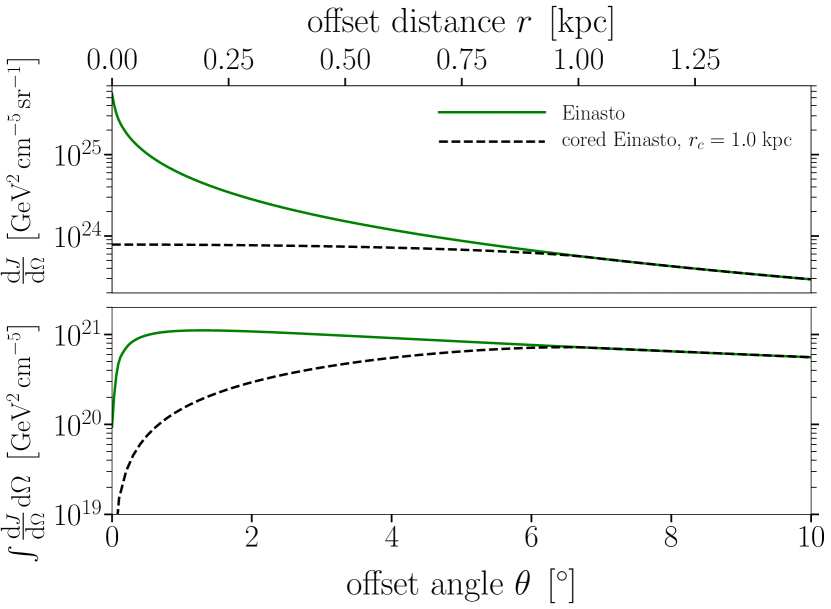
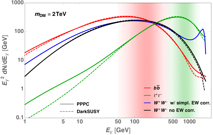
Figure 2: Left: Summary of $J-$factor profiles considered in this study, with solid (dashed) lines corresponding to the case of an Einasto (cored Einasto) profile for the DM density. The top panel shows the differential $J$-factor for an observation pointing an angle $\theta$ away from the GC (translating to a physical offset distance $r=r_{\odot}\tan\theta$), while the bottom panel shows the $J$-factor integrated over annuli of width $0.1^{\circ}$ as a function of the average annulus radius. Right: Summary of benchmark DM spectra adopted in this analysis for various final states, indicated by solid lines with different colours. Dashed lines show the corresponding spectra obtained with an alternative event generator. The shaded regions illustrate where the DM signal would be most important compared to a background that falls like a power law, $E^{-n_{\gamma}}$, with a fiducial value of $n_{\gamma}=2.7$ for the spectral index. For better visibility, these regions are only indicated for $b\bar{b}$ (red) and $\tau^{+}\tau^{-}$ (green) final states.

Spectral distribution

The dominant source of prompt gamma-ray emission from DM is expected to stem from the tree-level annihilation of WIMP(-like) particles into pairs of leptons, quarks, Higgs or weak gauge bosons. The primary annihilation products for non-leptonic channels then hadronise and decay, producing secondary photons mainly through the eventual decay of neutral pions. The resulting photon spectra ${dN_{\gamma}^{f}}/{dE_{\gamma}}$ for a given annihilation channel $f$ can be estimated with event generators like Pythia [111] or Herwig [112]. Owing to the large multiplicity of pions produced in the event chains, these spectra are typically of a rather universal form, lacking pronounced features apart from a soft fall-off towards the kinematical limit $E_{\chi}=m_{\chi}$ (see, e.g., Ref. [9]). For leptonic final states, in contrast, the production of pions is kinematically impossible (or, for $\tau^{+}\tau^{-}$, strongly suppressed). The result is a harder gamma-ray spectrum, from final state radiation in lepton decays, with a sharper cutoff at $E_{\chi}=m_{\chi}$.

The spectrum from a given two-body annihilation channel is in principle uniquely defined apart from intrinsic uncertainties originating from how different event generators implement the hadronisation and decay chains [113] . The dependence on the DM model enters the calculations explicitly when radiative corrections are taken into account, which lead to three- (or more) body final states (for a detailed discussion, see Ref. [114]). In particular, it is well known that an additional photon in the final state can both significantly enhance the annihilation rate and lead to very characteristic spectral features around the kinematic endpoint at $E_{\gamma}=m_{\chi}$ [115, 116, 62], while final state gluons only slightly change the photon spectrum expected from quark final states [117]. The effect of an additional electroweak gauge or Higgs boson in the final state has also been investigated in detail, again showing a large model-dependence for the resulting particle yields [118, 119, 120, 121, 122, 114]. When including electroweak corrections here, we will do so in a form that is sometimes referred to as ‘model-independent’ [123] (as implemented in the ‘Poor Particle Physicist Cookbook’, PPPC [124]). Specifically, the underlying assumption is that the contribution from weakly interacting bosons radiated from the initial DM states and virtual internal propagators can be neglected. This is, for example, satisfied in contact-type interactions of electroweak singlet DM; for Majorana DM like the supersymmetric neutralino, on the other hand, the resulting photon spectra can differ substantially [114]. It should also be stressed that all radiative corrections mentioned so far only concern leading order effects, and that there has recently been significant progress in including higher-order effects by consistently treating leading logarithms [65, 64, 69]. While these effects start to change the photon spectra appreciably for DM masses above the TeV scale, we will not take them into account here.

In the right panel of Fig. 2 we plot the photon spectra from PPPC for selected benchmark annihilation channels (solid lines). For the case of $W^{+}W^{-}$ the effect of the above-described implementation of electroweak corrections is largest; we therefore also indicate the spectrum without these corrections (which can be thought of as a very rough means of bracketing the model-dependence of such corrections). For comparison, we furthermore show spectra without electroweak corrections obtained from DarkSUSY (dashed lines). We note that for soft backgrounds that fall like $d\Phi/dE_{\gamma}\propto E^{-n_{\gamma}}$, with $n_{\gamma}\gtrsim 2$, the dominant contribution of these spectra to DM limits derives from the energy range where $E^{n_{\gamma}}_{\gamma}{dN_{\gamma}}/{dE_{\gamma}}$ (rather than ${dN_{\gamma}}/{dE_{\gamma}}$) peaks; we indicate this by shaded areas for typical soft ($b\bar{b}$) and hard ($\tau^{+}\tau^{-}$) channels, respectively. This demonstrates that, in the energy range relevant for our analysis, uncertainties due to different event generators, as well as how exactly simplified radiative corrections (in the above sense) are implemented, should not significantly affect DM limits – with the notable exception of the second peak that is expected [125] near the kinematical endpoint for $W^{+}W^{-}$ final states.

We finally remark that, in general, DM does not only produce prompt emission of gamma rays as described by Eq. (3.1). For typical annihilation channels, in particular, the same processes that produce prompt gamma rays also produce high-energy leptons, which leads to an inverse Compton (IC) component in gamma rays from the upscattering of cosmic microwave background (CMB) photons, thermal dust and starlight [126, 124]. For hadronic channels both the fraction and the distribution of energy that goes to electrons is comparable to that going into photons, but since the upscattered IC photons have on average significantly lower energy than the promptly produced gamma rays, the latter are much more easily discriminated against typical backgrounds (that fall with energy faster than the signal). Multi-TeV DM models annihilating to leptonic channels, on the other hand, and to some extent also $W^{+}W^{-}$ final states, produce sufficiently hard electrons to lead to a potentially distinguishable contribution of IC photons above the CTA threshold (see, e.g., Refs. [127, 128, 129]). Morphologically, however, the IC signal is much more diffuse (because TeV electrons propagate several hundred pc before being stopped [130]), and hence more difficult to model and detect against backgrounds. In fact, predicting the exact IC morphology requires detailed knowledge of both starlight distribution and electron propagation near the GC, thus introducing significant modelling uncertainty. Here we will therefore not include this component, but note that once there is evidence for a prompt DM emission signal, the detection of the associated IC component would provide a compelling cross-check of its nature.

3.2 Conventional astrophysics

Radio and X-ray data reveal the GC to be a very active region with non-thermal emitters such as star clusters, radio filaments and Sagittarius A* (see, e.g., Refs. [131, 132]). In gamma rays at energies below $100$ GeV the GC region is not significantly brighter than the rest of the Galactic plane [133] – despite the high number of confirmed energetic sources and the fact that this region contains about 10% of the total Galactic molecular gas content [132, 134, 135]. At TeV energies, on the other hand, IACT measurements have shown that the GC region clearly stands out, as described below [136, 137, 138, 139]. The astrophysical gamma-ray emission consists mainly of i) interstellar emission (IE) produced as secondary emission from CRs interacting with the interstellar medium (gas and dust, ISM) and fields (in particular the interstellar radiation field, ISRF), ii) localised gamma-ray sources (both individually resolved, and a cumulative emission from a sub-threshold population) and iii) possibly the emission from the base of the Fermi bubbles, all described in more detail below. Note that all these components (except for individually resolved sources) are extended and together also sometimes collectively referred to as Galactic Diffuse Emission (GDE).

Interstellar emission

The IE extends along the Galactic plane and is the brightest emission component in the Fermi-LAT data [133]. At high energies, the most relevant processes are i) CR interactions with the ISM gas, producing gamma rays predominantly through the neutral pion channel, and ii) IC scattering, in which CR electrons up-scatter ISRF and CMB photons to gamma-ray energies. These two components have distinct morphologies: the first, so-called ‘hadronic emission’ tracks that of the gas, while the morphology of IC emission is determined by the distribution of CR leptons and the ISRF. Theoretical modelling of the IE emission depends on a significant number of parameters related to the injection spectra of CRs, their spatial distribution in the Galaxy, diffusion properties but also properties of the interstellar medium and ISRF. This implies a high level of modelling uncertainty, adding to significant degeneracies between some of the involved parameters (for a review see Ref. [133]).

Despite its relative brightness, the spatial extension of the IE has made it notoriously difficult to be detected with IACTs (partially motivating efforts to determine TeV diffuse emission using the decade-long exposure of Fermi-LAT [140]). Notable progress has been made by H.E.S.S. through the detection of a bright diffuse gamma-ray emission from the so-called Galactic Ridge, originating from dense molecular clouds in the central 200 pc [136, 137, 138], as well as that of cumulative emission from the Galactic plane (providing latitude and longitude profiles, but not spectral information [141]). Advances in determining the large-scale diffuse emission along the Galactic plane have also been made by water-Cherenkov telescopes at higher energies, first with MILAGRO [142] and more recently with HAWC [143], though mostly at longitudes $\gtrsim 30^{\circ}$ due to the geographical location of these instruments. CTA is expected to spatially resolve large-scale emission at TeV energies with unprecedented precision and angular resolution. We will test a set of specific IE models (IEMs) to gauge the impact of the associated modelling uncertainties on the sensitivity to a DM signal. These models are chosen to sample a representative range of realistic theoretical possibilities, given the current state of knowledge:

• Gaggero et al. [144] studied diffuse models that can simultaneously explain H.E.S.S. data in the region of the Galactic Ridge, and Fermi-LAT data in the surrounding region, at lower energies. They discuss two possibilities to reconcile these measurements:

  • The Base model rests on often-adopted, simplifying assumptions concerning CR diffusion, and in particular assumes a constant diffusion coefficient across the Galaxy. The large scale diffuse emission measured by Fermi-LAT and the emission from the Galactic Ridge (H.E.S.S.) then must have a different origin, with the latter postulated to originate from a so-far unknown source related, e.g., to transient emission from the GC. In our analysis, we thus simply add the H.E.S.S. Ridge template [136] to the original form of the Base model (see also Appendix B.1). The large-scale emission predicted in this model is very soft, nominally already in some tension with the Fermi-LAT data [144] (which would be alleviated in the presence of yet another emission component like, e.g., unresolved sources).

  • The Gamma model relaxes the assumption of a spatially constant CR diffusion coefficient, allowing instead for a radial dependence where diffusion is more efficient closer to the GC. This implies harder and brighter gamma-ray emission in the innermost Galactic regions, explaining simultaneously the bright Galactic Ridge in the very centre and the large scale diffuse emission measured by Fermi-LAT. This model predicts a relatively bright emission also outside the ridge.

• The Pass-8 Fermi IEM was derived based on the detailed analysis of 8 years Pass 8 Fermi-LAT data. Special care was taken for the model to describe the high-energy ($\geq 50$ GeV) spectrum, and it is, therefore, more reliable regarding high energy extrapolation than previous versions. It uses different gas maps than the Gaggero et al. models and is tuned to the LAT data over the entire sky (as opposed to the Base model, which is more heavily based on theoretical expectations).

Resolved and sub-threshold sources

The Galactic plane survey of the H.E.S.S. collaboration has discovered six TeV-bright objects in the GC region [145], that were later studied also with MAGIC and VERITAS. In particular, G0.9+0.1, HESS J1745-290 and HESS J1741-302 are best fit as point sources, while HESS J1745-303 and HESS J1746-308 are extended sources (with an extension of $0.2^{\circ}$ and $0.15^{\circ}$, respectively[137]); G0.9+0.1 is identified as a composite supernova remnant hosting a PWN in its core (see also the VERITAS analysis [138]) while HESS J1745-290 coincides with the position of Sagittarius (Sgr) A^∗ (c.f. further characterisations by MAGIC [146] and VERITAS [138]), the supermassive black hole at the centre of the MW. The sixth source, HESS J1746-285, is very close to two TeV-emitting sources detected by VERITAS [138] and MAGIC [146]. However, as reported by H.E.S.S. [137], this source is possibly the combination of a part of the Galactic ridge and a yet unknown emitter. Hence, we do not consider this source in our analysis. For the remaining five sources we adopt circular masks centred on the respective source position (taken from Ref. [137]), with an energy-independent radius of $0.3^{\circ}$ for point sources and $0.6^{\circ}$ for extended sources. Our masking scheme is indicated in Fig. 1.

The Galactic centre region presumably also houses many sources that are too faint to be detected with the current generation of IACTs, as well as a component of even fainter sources, below the CTA detection threshold, that will contribute to the diffuse emission. For example, while the Fermi-LAT catalogue of hard sources (2FHL[147]) lists no sources in our ROI, 4FGL [148] lists 16 identified sources, three of which are tagged as candidate TeV emitters listed in the online TeV source catalogue TeVCAT [48]. Since the CTA source detection threshold is still unknown especially in crowded regions like the Galactic centre, we will use a single template for all but the brightest sources detected by current IACTs.

Given that there are only a few TeV sources currently known in the region, predicting the contribution of faint sources comes with considerable uncertainty. Within the context of the CTA Galactic plane survey, significant consortium effort has recently gone into modelling the population properties of the most numerous Galactic TeV sources (PWNe, SNRs and binaries) [149]. We use the gamma-ray templates derived in that work (applying a $\mu$Crab lower flux threshold, while for the higher flux cut-off we used the detection threshold from the H.E.S.S. Galactic plane survey, [150], namely, for the GC region, a flux of 5 mCrab at energies $>400$ GeV) and refer for all details to that upcoming publication. We will discuss the impact of that template on our analysis in Sec 6.2.

Fermi bubbles

The gamma-ray emission from the Fermi bubbles (FB) has been studied extensively since their discovery in 2010 [151, 152]. Even though the FB outshine the IE at high latitudes due to their hard spectrum, their shape close to the Galactic plane is challenging to distinguish from the bright IE. Here we will rely on a recent analysis [153] determining the morphology and spectrum at the base (i.e. the low-latitude part) of the FB, and use these spatial and spectral templates to gauge the potential impact of the FB on the search for DM signals. A projection of CTA’s sensitivity to the base of the FB based on the same spatial and spectral template has been derived in Ref. [154]. We stress however that the exact shape and spectra of the FB close to the GC are highly uncertain – though a re-examination of the FB base using nine years of LAT data [155] confirmed the previously reported hard power law without indications of a cutoff up to energies of 1 TeV.

3.3 Residual cosmic-ray background

CR events misidentified as gamma rays make up the highest portion of detected events, outshone only by the brightest sources. The core of the issue is that the CR proton (electron) fluxes are $10^{4}$ ($10^{2}$) times higher than the diffuse flux of gamma rays expected from the Galaxy (at $\sim 100$ GeV). While hadron-induced showers can be distinguished from electromagnetic showers based on their shape, with an (energy-dependent) background rejection rate better than $10^{-2}$, CR electrons present an essentially irreducible background (preliminary studies indicate that some rejection may be possible [156], but not on short time scales). Besides, while the spectrum of CR protons and electrons is well measured below a few TeV [157, 158, 159, 160], significant uncertainties about the number of events passing all analysis cuts remain, making the exact spectrum and normalisation of this intrinsically isotropic component challenging to model (the measured distribution of events within CTA’s field of view, in contrast, is determined by the instrument response to cosmic-ray background, which is not isotropic – especially at high energies). On top of this, the atmosphere itself, acting as an effective calorimeter, introduces additional uncertainties.

We will see, however, that uncertainties in isotropic parts of the background components mostly affect our analysis by changing the signal-to-noise ratio, which in fact turns out to be a subdominant effect. A bigger impact on the DM sensitivity results from varying (in time and space) unresolved backgrounds, for example small-scale anisotropies in an otherwise largely isotropic emission. These could originate, for example, by the presence of aerosols in the atmosphere which can also introduce a strong bias in energy reconstruction and deteriorate the energy resolution (even though this is to some degree addressed by dedicated studies of atmospheric conditions by CTA monitoring instruments).

In our analysis, the modelling of the misidentified CR component relies on extensive Monte Carlo simulations of CR showers and their subsequent event reconstruction, allowing us to obtain the expected number of CR misidentified events for a given set of IRFs. (This is in contrast to the more conventional ‘ON/OFF’ technique which does not rely on MC simulations and makes it instead possible to adjust the CR background model directly to the data; see, e.g., Ref. [162, 163].) The underlying IRFs do not include small-scale anisotropies (which is an issue shared with the ON/OFF technique), which might be present in the real data due to, e.g., uneven atmospheric conditions. Because the corresponding systematic uncertainties have not yet been studied in detail, we will include them in a parametric way (as described in Section 4).

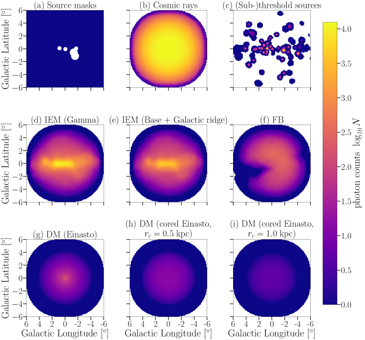
Figure 3: Background and signal templates computed by ctools for the GC survey observation, showing the expected photon counts in the energy range from 100 to 500 GeV. The (logarithmic) colour code indicates the number of expected counts $N$ per $0.1^{\circ}\times 0.1^{\circ}$ pixel. See text for a description of each of the individual templates shown here.

3.4 Emission templates and caveats

To summarise our discussion of emission models, we compare in Fig. 3 the total count maps in the 100 – 500 GeV range that result from our benchmark emission templates (as generated by ctools, for the GC survey mode described in Section  2.2). From top left to bottom right, these correspond to:

• residual CR background events, generated from prod3b-v1 IRFs (Section 2.2)

• interstellar emission, as predicted in the Gamma and the Base model (Section 3.2)

• a realisation of sub-threshold sources (Section 3.2)

• the Fermi bubbles (Section 3.2)

• the DM emission template (Section 3.1) for the Einasto profile with and without a constant density core, as indicated. For definiteness we choose here $m_{\chi}=2$ TeV for the DM mass, and an annihilation cross-section $\langle\sigma v\rangle=3\times 10^{-26}\;\textrm{cm}^{3}\textrm{s}^{-1}$ to $b\bar{b}$ final states.

In Fig. 4 we show the energy dependence of the various components, by plotting the total number of expected counts, during the entire Galactic centre survey observation, per energy bin. We first note a relatively sharp increase in the number of counts for all components at energies $\gtrsim 60$ GeV; the origin of this feature is a corresponding increase in the effective area of the array, as we pass above the MST energy threshold. When it comes to the comparison of the various physical components, furthermore, Figs. 3 and 4 call for a number of pertinent comments:

1. CR contamination clearly dominates all other emission components. The CR electron flux up to TeV energies has been well-measured by a number of instruments, including AMS-02 [157], the Calorimetric Electron Telescope (CALET) [159], and the Dark Matter Particle Explorer (DAMPE) [160].  In the figure we show the DAMPE spectrum to guide the eye as to the level of expected background. CR electron fluxes constitute, as discussed in Section 3.3, an essentially irreducible background to gamma-ray searches. Given the importance of electrons up to the TeV energy range, it thus will be particularly hard to further improve the CR rejection efficiency at these energies.

2. The Gamma and Base IEMs are based on the same target gas and ISRF maps, but on different assumptions concerning CR diffusion. This results both in different spectra and in different morphologies, with the Gamma model being significantly brighter in the central regions. For comparison, Pass 8 Fermi IEM (only shown in Fig. 4, not in Fig. 3) features a flux very similar in spectrum and normalisation to that of the Gamma model, however it is based on different target gas and ISRF maps, as well as on different assumptions about CR diffusion (the morphologies of templates based on different IEMs are compared in more detail in Appendix B.2).

3. Unresolved sources and FB are among the most uncertain emission components, and a mis-modelling of their morphology could potentially mimic, at least partially, the DM template. This is aggravated by the fact that the fluxes of these components are at least comparable to that from the annihilation of thermally produced DM. Potentially, this could thus have a significant impact on DM searches, causing fake signal detections or artificially strong limits. Note that a separate study of sub-threshold sources for CTA is still ongoing and we hence only use the specific realisation of such a population shown in Fig. 3c; the eventual analysis of real data, beyond the scope of this work, will have to be based on an average over many sub-threshold source realisations. We return to these issues in Section 6.

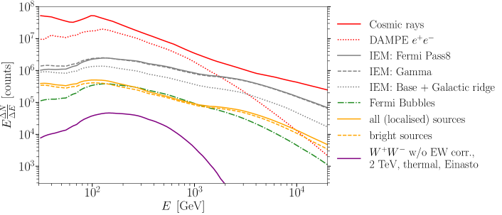
Figure 4: Differential counts (per bin) expected from the GC survey, multiplied by the bin energy $E$, for the emission components considered in this work – including the total CR background (from electrons and hadrons, solid red line), three alternative IE models, localised source components (both bright individual sources and unresolved sources), Fermi bubbles and the DM spectrum (assuming $m_{\chi}=2$ TeV, $\langle\sigma v\rangle=3\times 10^{-26}\;\textrm{cm}^{3}\textrm{s}^{-1}$ and dominant annihilation to $W^{+}W^{-}$). For a very rough translation of these counts to fluxes, one needs to divide by the CTA effective area ($9\cdot 10^{5}$ m² at 1 TeV [53]), the angular size of our analysis ROI (0.037 sr, not including direction cuts) and the total observation time of 525 h.

We conclude this section by mentioning another aspect of astrophysical modelling that may appear as a relevant issue once the analysis chain is confronted with real data, but which would be premature to include in the present modelling of emission components given the current lack of knowledge and robust data. The IC component of the interstellar emission, in particular, is more difficult to model since it does not, unlike hadronic emission, correlate with gas maps. Besides, the IEMs used here (and more generally in the majority of the relevant literature) assume steady-state solutions for CR propagation, based on smoothly distributed source populations. That assumption is expected to fail at energies $\gtrsim 100$ GeV because of the small energy loss time of electrons, implying that the morphology of the IC emission changes significantly and becomes sensitive to the CR electron injection history [164]. In particular, electrons are contained closer to the sources, which in turn introduces a significant granularity in the IC templates and lowers the strength of large-scale IC emission by up to about $30\%$ [164]. While the latter effect would facilitate the detection of a DM signal, the former (i.e. the difficulty to model overlapping ‘point-like’ emission sources) could present a non-negligible challenge for future DM searches at these energies. We leave a more detailed study of these aspects for future works, but note that the difference between Base and Gamma models should capture (in part) the impact of the latter effect on the DM sensitivity.

4 Data Analysis

The traditional way to constrain DM annihilation with IACTs is the so-called ON/OFF approach (e.g. [17, 15, 14, 165, 12]), which rests on the definition of two spatially separate, different kinds of ROIs (often within the same FoV): in the ‘ON’ region the signal is expected to be the strongest while in the ‘OFF’ region it is expected to be subdominant. Under the hypothesis that we know how the background scales between OFF and ON regions (solid angle/acceptance effects are routinely corrected for; see, for instance, the $\kappa$ factors in Eq. (C.2)), it is, in principle, possible to measure the background under the same observational conditions. Such an approach is complementary to template-based morphological analyses, more typical in the context of satellite-borne instruments (e.g. [166]), where different emission components are described by templates that are fitted to binned data. While the template analysis offers the possibility to incorporate spatially varying backgrounds, there can be a remaining systematic uncertainty related to the exact form of the adopted templates (for attempts to address these limitations see e.g. SkyFACT [167]). Possible reasons for not using the template approach in most past IACT analyses include i) their relatively small FoV ii) the residual CRs being the only background component, assumed to be effectively the same in the ON and OFF regions at the energies of interest here; and iii) the complexity of robustly modelling this background.

Only more recently it was realised that template fitting may be a powerful technique for the analysis of IACT data [162, 163] (see also Ref. [17] for a ’hybrid’ approach). To fully exploit the power of CTA with its larger FoV, higher background rejection and higher flux sensitivity compared to previous experiments, and to achieve a corresponding increase in DM sensitivity, the background needs to be modelled in higher detail and with more components than required for current instruments. So far, astrophysical modelling was not done in a very detailed way and CR uncertainties were mostly treated in a simplified manner [14, 25]. One of the main motivations of this work is to study the applicability of the template fitting approach in detail (later, in Appendix C.4, we will also directly confront this method with the traditional ON/OFF approach).

Template Analysis

We employ a binned likelihood based on Poisson statistics $\mathcal{L\!}\left(\left.\bm{\mu}\right|\bm{n}\right)=\prod_{i,j}e^{-\mu_{ij}}{\mu_{ij}^{n_{ij}}}/{\left(n_{ij}\right)!}$, where $\bm{\mu}=\{\mu_{ij}\}$ denotes the model prediction and $\bm{n}=\{n_{ij}\}$ the (mock) data counts, for bins in energy (indicated by an index $i$) and angular position on the sky (indicated by an index $j$). The model is given by a set of background templates as shown on Fig . 3, $\{\mu_{ij}^{X}\}$, a signal template for the DM component, $\mu_{ij}^{\chi}$, and normalisation parameters $\bm{A}$ for the relative weight of these templates:

$$\mu_{ij}(A^{\chi},A^{X}_{i})=A^{\chi}\mu_{ij}^{\chi}+\sum_{X}A^{X}_{i}\mu_{ij}^{X}\,.$$ (4.1)

For any given signal template – defined by the adopted DM density profile and annihilation spectrum – we thus introduce a global normalisation parameter $A^{\chi}$ that is directly proportional to the annihilation strength $\langle\sigma v\rangle$ that we want to constrain, c.f. Eq. (3.1). For the background components $X$ – CRs, IE, Fermi bubbles and unresolved sources, depending on the analysis benchmark – we instead adopt normalisation parameters $\{A^{\rm X}_{i}\}$ that may vary in each energy bin, where $A^{\rm X}_{i}\equiv 1$ corresponds to the (expected) default normalisation of the templates as summarised in Section 3.4. This ansatz accounts in an effective way for uncertainties in the spectral properties of the templates, thereby rendering the resulting DM limits more conservative. It should be stressed that by construction this method thus relies more on the morphological than on the spectral information in the templates, which is partially motivated by the excellent angular resolution of CTA. We will discuss this point in more detail below when explicitly introducing systematic uncertainties. Mock data, finally, are prepared for each of the background components $X$ by drawing the number of photon counts in a given bin, $n_{ij}^{X}$, from a Poisson distribution with mean $\mu_{ij}^{X}$. Summing these contributions then gives the total number of counts per bin, $n_{ij}=\sum_{X}n_{ij}^{X}$.

We generate all count maps using ctools. As our benchmark binning scheme we choose – unless explicitly stated otherwise (see also Section 6.1 for a discussion) – square spatial bins of width $0.1^{\circ}$, roughly corresponding to the typical PSF, and 55 spectral bins in the range from 30 GeV to 100 TeV chosen such that their width is given by the energy resolution at the central bin energy, at the two standard deviations ($2\sigma$) level. We restrict our analysis to circular FoV regions with a radius of 5^∘ around the respective pointing direction of the array (c.f. Fig. 1).

To derive an upper bound on the DM normalisation $A^{\chi}$, for a fixed DM template $\bm{\mu}^{\chi}$ and a given data set $\bm{n}$, we define the test statistic

$$\textrm{TS}\!\left(A_{\chi}\right)=\min_{\{A_{i}^{X}\}}\left(-2\ln\!\left[\frac{\mathcal{L}\!\left(\left.\bm{\mu}(A^{\chi},A_{i}^{X})\right|\bm{n}\right)}{\mathcal{L}\!\left(\left.\bm{\hat{\mu}}\right|\bm{n}\right)}\right]\right)\,,$$ (4.2)

where $\bm{\hat{\mu}}\equiv\mu(A^{\chi}=\hat{A}^{\chi},A^{X}_{i}=\hat{A}^{X}_{i})$ denotes the model counts in Eq. (4.1) for the best-fit values of all normalisation parameters (i.e. both for DM and background components) obtained by maximising the likelihood. This test statistic is distributed according to a $\chi^{2}$-distribution with one degree of freedom [168], so a (one-sided) upper limit on $A^{\chi}<A^{\chi}_{\mathrm{max}}$ at $95\%$ ($99\%$) Confidence Level (C.L.) corresponds to a TS value of 2.71 (5.41).

It is straightforward to extract the mean expected limit, $\langle A^{\chi}_{\mathrm{max}}\rangle$, and its variance, $\sigma^{2}=\langle A^{\chi}_{\mathrm{max}}-\langle A^{\chi}_{\mathrm{max}}\rangle\rangle^{2}$, by compiling Monte Carlo realisations of mock data sets, and then take limits for each of those according to the above prescription. As this is computationally rather intensive, however, we will instead typically utilise a single ‘representative’ set of data, the so-called Asimov data set, $\bm{n}_{A}$: for a Poissonian process, this corresponds to the expected number of counts per bin one would obtain with an infinitely large sample of individual Poisson realisations of a given background or signal model, i.e. $\bm{n}_{A}=\mu(A^{\chi}=0,A^{X}_{ij}=1)$ [169]. In principle, this approach can also be used to estimate the variance of the expected upper limits. However, we checked that in its simplest implementation [169] this does not lead to a reliable estimate once systematic uncertainties (to be discussed below) are taken into account; whenever we present ‘sidebands’ to expected limits, these are thus based on full Monte Carlo calculations.

Treatment of Systematic uncertainties

For a future experiment, instrumental systematic uncertainties are by nature hard to quantify. However, we can still estimate the possible effects in a general manner by introducing uncertainties that are correlated among the data bins (as is typical for instrumental systematic errors). Similarly, correlated systematic errors can also account for additional systematic uncertainties in the IEM templates that are not already captured in the template analysis. Such correlated uncertainties may partially degrade morphological differences of the background/signal templates and, hence, weaken their constraining power over the signal component.

Correlated Gaussian uncertainties (with zero mean) are fully defined in terms of their covariance matrix, $K$. For our purposes, this may encompass

• spatial bin – spatial bin correlations,

• energy bin – energy bin correlations and/or

• spatial bin – energy bin correlations.

As described below, we will only consider the first two types of correlations. To apply the covariance matrix description of systematic errors, we follow the approach outlined in Refs. [170, 171], and implemented in the publicly available Python package swordfish [172]. In particular, we change the construction of the model prediction in Eq. (4.1) (but not that of the data $\bm{n}$) in the following way: Instead of varying the background templates by normalisation parameters $A_{i}^{\rm X}$ per energy bin to account for background fluctuations, we set these normalisation parameters to unity and explicitly introduce Gaussian ‘background perturbations’ $\Delta B$ – related, e.g., to uncertainties of the reconstruction of events – for each individual template bin $k$,

$$\left(\mu_{K}\right)_{k}\equiv\sum_{X}\mu_{k}^{X}+\Delta B_{k}+A^{\chi}\mu_{k}^{\chi}\,.$$ (4.3)

Here, the sum runs over the model templates $X$ to be examined, the index $k$ comprises both spatial and energy bins, i.e. $k\in[1,\mathcal{N}]$ with $\mathcal{N}$ being the product of the number of spatial pixels and the number of energy bins. In principle, the different templates can give rise to different background perturbations, i.e. $\Delta B_{k}=\sum_{X}\Delta B_{k}^{X}$. Including the Gaussian prior on the background variations $\Delta B_{k}$ in the likelihood function (and neglecting a constant determinant) then yields

$$\mathcal{L\!}\left(\left.\bm{\mu}\right|\bm{n}\right)=\prod_{k=1}^{\mathcal{N}}\frac{\mu_{k}^{n_{k}}}{\left(n_{k}\right)!}e^{-\mu_{k}}\times\exp\!\left[-\frac{1}{2}\Delta B_{k}\sum_{l=1}^{\mathcal{N}}\left(K^{-1}\right)_{kl}\Delta B_{l}\right]\,,$$ (4.4)

where $K_{ij}\equiv\langle\Delta B_{i}\Delta B_{j}\rangle$ is the covariance matrix (and we assume $\langle\Delta B_{i}\rangle=0$). Profiling over the nuisance parameters $\Delta B_{i}$, this reduces to a log-likelihood function that only depends on the signal normalisation $A^{\chi}$ (again omitting terms that are constant in the model parameters):

$$-2\ln{\mathcal{L}\!\left(\left.\bm{\mu_{K}}\right|\bm{n}\right)}=\min_{\bm{\Delta B}}\left\{\sum_{k=1}^{\mathcal{N}}\left[\vphantom{\int}n_{k}\ln{\left(\mu_{K}\right)_{k}}-\left(\mu_{K}\right)_{k}\right]-\frac{1}{2}\sum_{k,l=1}^{\mathcal{N}}\left[\vphantom{\int}\Delta B_{k}\left(K^{-1}\right)_{kl}\Delta B_{l}\right]\right\}\rm{.}$$ (4.5)

For systematic uncertainties that are uncorrelated between the background templates $X$, which is the case we consider here, we have $\langle\Delta B_{i}^{X}\Delta B_{j}^{Y}\rangle=0$ for $X\neq Y$. The last term in the above equation can then be written as $\sum_{k,l}\Delta B_{k}\left(K^{-1}\right)_{kl}\Delta B_{l}=\sum_{X}\sum_{k,l}\Delta B_{k}^{X}\left(K^{-1}\right)^{X}_{kl}\Delta B^{X}_{l}$, where $K=\sum_{X}K^{X}$ is now understood to be the total correlation matrix.

Upper limits on the DM signal are derived by constructing a test statistic in full analogy to Eq. (4.2), mutatis mutandis. Concerning the concrete construction of covariance matrices, the simplest way to parameterise spatial correlations is by an $\mathcal{N}_{\rm S}\times\mathcal{N}_{\rm S}$ matrix $K_{\rm S}$, with

$$\left(K_{\rm S}\right)_{jj^{\prime}}=\sigma_{{\rm S}}^{2}\exp\!{\left(-\frac{1}{2}\frac{\left\lVert\vec{r}_{j}-\vec{r}_{j^{\prime}}\right\rVert^{2}}{\ell_{\rm S}^{2}}\right)}\rm{,}$$ (4.6)

where $\mathcal{N}_{\rm S}$ refers to the number of spatial bins in the ROI, $\sigma_{{\rm S}}$ denotes the magnitude of the spatial systematic uncertainty, $\ell_{\rm S}$ the spatial correlation length, $\vec{r}_{j}$ is the central position of the $j-$th spatial template bins in degrees of Galactic longitude and latitude, and we use the norm on the unit sphere for the distance between two spatial bins. $\sigma_{{\rm S}}$ and $\ell_{\rm S}$ may in general depend on the position in the template but, for simplicity, we assume them to be constant here. By analogy, energy correlations can be parameterised by an $\mathcal{N}_{\rm E}\times\mathcal{N}_{\rm E}$ matrix

$$\left(K_{\rm E}\right)_{ii^{\prime}}=\sigma_{{\rm E}}^{2}\exp\!{\left[-\frac{1}{2}\left(\frac{\log_{10}\!{\left(E_{i}/E_{i^{\prime}}\right)}}{\ell_{\rm E}}\right)^{2}\right]}\,,$$ (4.7)

where $\mathcal{N}_{\rm E}$ refers to the number of energy bins, $\sigma_{{\rm E}}$ denotes the magnitude of the spectral systematic uncertainty, $\ell_{\rm E}$ the energy correlation length (in dex, i.e. per decade) and $E_{i}$ is the central value of the $i-$th energy bin. In general, the covariance matrix is then given by the tensor product $K=K_{\rm E}\otimes K_{\rm S}$. In our analysis, however, we will restrict ourselves to considering correlations of type (i) and (ii) from the aforementioned list, which can be understood as particular instances of the most general case. They can be constructed as follows:

• $K_{S}$ describes correlations among the spatial template bins. To exclude any further energy correlation between different energy bins, one has to assume an infinitesimally small energy correlation length $\ell_{E}$. Thus, $K_{E}$ should be diagonal, i.e. each energy bin is exclusively correlated to itself. In other words, the full covariance matrix is the tensor product of the identity matrix in energy space and $K_{S}$, $K=\mathbb{I}\otimes K_{S}$.

• Spectral correlations among a template’s energy bins are described by $K_{E}$. In this case, however, one cannot assume an infinitesimally small spatial correlation length to describe the full matrix $K$: otherwise $K_{E}\otimes\mathbb{I}$ would predict a correlation of every spatial bin with its own copy in different energy bins, allowing the spatial bins to vary independently of each other and thereby erase the morphological information one wants to preserve. Instead, one needs to assume an infinitely large spatial correlation length such that all spatial bins are varied as an ensemble, i.e. $K_{S}$ must be chosen as a dense matrix where every element is equal to 1.

As a default assumption, we will adopt a 1% overall normalisation error (corresponding to one of the design requirements of CTA [12]), $\sigma_{S}=0.01$, and a spatial correlation length of $\ell_{S}=0.1^{\circ}$ (roughly motivated by the typical size of the PSF). We also do not explicitly assume any energy correlations in the default analysis pipeline, as these turn out to affect our analysis much less. All these choices will be explicitly revisited and discussed in Section 6.1.

ON/OFF analysis

For comparison with the more traditional approach, we also perform a likelihood analysis with the same energy binning as in the template approach, but effectively using spatial bins with a ring morphology (implemented as multiple ON regions). Here we do not model the background components as above (because the background is by definition determined in the OFF region), so the total joint-likelihood function $\mathcal{L}$ is a function of only two parameters, namely the DM mass $m_{\chi}$ and the velocity-weighted annihilation cross section $\langle\sigma v\rangle$. Our construction of ON and OFF regions near the GC closely follows that by H.E.S.S. [165, 173], adapted to the planned GC survey of CTA. We provide further analysis details in Appendix C.4, and discuss how this approach compares to the results from our baseline analysis strategy based on template fitting – with particular emphasis on the fact that CTA is also expected to pick up astrophysical ‘signal’ components that most likely are different in the two ROIs.

5 Projected dark matter sensitivity

In this section we present the main results of our analysis, namely the sensitivity of CTA to a DM signal, focussing exclusively on the following benchmark settings:

• GC survey observation strategy, masking bright sources as indicated in Fig. 1.

• Asimov mock data set based on CR background and IE Gamma model templates.

• Template fitting analysis based on $0.1^{\circ}\times 0.1^{\circ}$ spatial bins and 55 energy bins between 30 GeV and 100 TeV (and a width corresponding to the energy resolution at the $2\sigma$ level). Our default treatment of systematic uncertainties implements a 1% overall normalisation error and a spatial correlation length of $0.1^{\circ}$ (but no energy correlations).

In the subsequent Section 6, we will discuss how our results are affected by modifying the benchmark assumptions listed above.

5.1 Expected dark matter limits

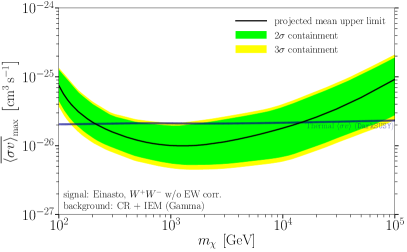
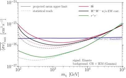
Figure 5: Sensitivity of CTA to a DM annihilation signal, at 95% C.L., based on our benchmark treatment of the expected instrumental systematic uncertainty. Following common practice, this is presented in terms of projected mean upper limits on the average velocity-weighted annihilation cross section, as a function of the DM mass $m_{\chi}$. Solid lines show the sensitivity based on our benchmark settings, while dashed lines show the reach assuming no systematic uncertainty in the spatial templates. We also indicate the ‘thermal’ cross-section that for the simplest DM models leads to a relic density within the $3\sigma$ range of the DM abundance observed by Planck [1, 174]. Left panel: Sensitivity to DM annihilation into $W^{+}W^{-}$ final states (black), without electroweak corrections (see Section 3.1 for a discussion). The green (yellow) band indicates the $2\sigma$ ($3\sigma$) scatter of the projected limits (based on Monte Carlo realisations). Right panel: DM annihilation into $\bar{b}b$ (red), $W^{+}W^{-}$ (black) and $\tau^{+}\tau^{-}$ (green), respectively.

.

The most often considered ‘pure’ annihilation channels for heavy DM candidates are those resulting from $\bar{b}b$, $W^{+}W^{-}$ and $\tau^{+}\tau-$ final states (in the order of increasingly harder spectra). In Fig. 5 we show the expected limits for DM models where annihilation into these final states dominates, for a DM template based on the Einasto DM profile given in Eq. (3.3). For comparison, we also indicate the cross-section needed to thermally produce DM in the early universe in order to match the cosmologically observed DM abundance. Specifically, we use DarkSUSY to calculate this cross-section, following the treatment of Ref. [73] under the assumption of self-conjugate DM particles annihilating with a velocity-independent $\sigma v$. We thereby improve upon similar recent results [175, 105] by using an updated temperature dependence of the number of relativistic degrees of freedom during and after freeze-out [176] and the newest Planck data for the observed value of $\Omega_{\chi}h^{2}=0.120$ [1, 174].

We see from Fig. 5 that CTA indeed has the potential to test the ‘thermal’ annihilation cross-section for a wide range of DM masses, in particular for the slightly harder gamma-ray spectrum that results from $W^{+}W^{-}$ final states. As pointed out in the introduction, this makes CTA perhaps the most promising instrument to test the WIMP paradigm for DM masses at the TeV scale, providing indeed one of its major science cases. Let us stress that we confirm this expectation after including our benchmark treatment of systematic uncertainties – which we consider realistic given the obvious limitation that our analysis describes an instrument yet to be built (see Section 6.1 for a discussion). For comparison, we also indicate the mean projected limits that would result if only statistical errors were included in the analysis. As expected, limits are not affected in the statistics-limited case of the low photon counts in models with large DM masses (as well as the background components at these high energies). For DM masses significantly below 10 TeV, on the other hand, the limits clearly become dominated by systematic uncertainties rather than by statistical errors because, for a given annihilation cross-section, both the background and the signal fluxes are much higher.

5.2 Generalised flux sensitivities per energy bin

Actual spectra for a given DM model rarely coincide exactly with those of the ‘pure’ channels discussed above. While the use of ‘pure’ channel limits is standard practice, limits as presented in Fig. 5 thus have reduced practical applicability. In Fig. 6 we therefore provide limits to the (spatial) DM template in a different way, more independent of the spectral model. Concretely, we show energy-flux sensitivities obtained by applying the likelihood function defined in Eq. (4.5) per energy bin. Here we assumed for simplicity that the flux is described by a power law $\textrm{d}\Phi/\textrm{d}E\propto E^{-2}$ rather than following one of the explicit annihilation spectra considered above. As expected (and checked explicitly) the spectral form has only a minor effect on the result because the per bin contribution to the total likelihood is mostly affected by the photon count inside that energy bin (provided the bins are, as in our case, chosen sufficiently small [177]). This makes this result more universal, motivating us to also indicate the change in the full likelihood $\mathcal{L}_{i}$ per energy bin (and to make it available in tabulated form [178]). To a reasonable approximation, this can be used to constrain the signal normalisation, at 95% C.L., of an almost arbitrary smooth DM spectrum $dN_{\gamma}/dE_{\gamma}$, where $N_{\gamma}$ is the number of photons per annihilation process. Concretely, this corresponds to requiring

$$\sum_{i}\Delta\ln\mathcal{L}_{i}\left[C_{\chi}E_{i}\,dN/dE_{\gamma}\right]<2.71\,,$$ (5.1)

where the sum runs over all energy bins, with central energy $E_{i}$, and the correct flux normalisation is ensured by using

$$C_{\chi}\simeq\left(2.5\cdot 10^{21}\;\textrm{GeV}^{2}/\right.\left.\textrm{cm}^{5}\right)\times\langle\sigma v\rangle_{\mathrm{ann}}\,S_{\chi}^{-1}m_{\chi}^{-2}\,,$$ (5.2)

c.f. Eq. (3.1). For DM spectra varying more strongly with energy than $E^{-2}$, integrating over the energy inside each bin, rather than using the mean number of photons in each bin as in Eq. (5.1), would provide a slightly more accurate estimate (while highly localised spectral features, such as monochromatic gamma-ray lines [10], would warrant a different analysis strategy that leads to significantly better limits than indicated in Fig. 6 [179]). Let us stress that we provide here the tabulated binned likelihoods $\mathcal{L}_{i}$ only for convenience, to allow for quick and simple estimates of sensitivities to DM models not covered in our analysis; all our results are based on the full procedure detailed in Section 4 rather than on the ‘short-cut’ defined by Eq. (5.1).

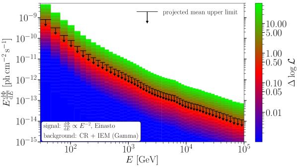
Figure 6: Differential flux (times $E$) as a function of source energy $E$. The (logarithmic) colour scale shows the change in the total likelihood due to the contribution from a DM signal in the respective energy bin, assuming a DM-induced flux locally scaling as $\textrm{d}\Phi/\textrm{d}E\propto E^{-2}$. To guide the eye, the black symbols indicate the value of $\Delta\log\mathcal{L}$ that corresponds to a $2\sigma$ upper limit on such a DM signal, from a single bin. Limits on DM models with arbitrary spectra, taking into account all energy bins, can be approximated as in Eq. (5.1). The full likelihood table is available for download at zenodo [178].

5.3 Extended dark matter cores

Let us now address the impact of the assumed DM density profile. We re-iterate from the discussion in Section 3.1 that the Galactic DM distribution within the inner few kpc (and even more so for $r\ll 1$ kpc) is rather uncertain and not very well observationally constrained – but at the same time the distribution is crucial for estimating the overall strength of the annihilation signal. The situation in the GC is, in general, different from the situation in dwarf spheroidal galaxies, where kinematic data allow us to constrain the $J$-factor sufficiently [180] to warrant including them in the likelihood analysis, fully marginalising over the profile parameters [181, 182, 183]. One of the reasons behind this is that for dSphs we typically observe the entire DM halo and therefore the full ‘bolometric’ DM emission which – unless considering extreme examples – only depends weakly on the DM density profile [184] (for the GC, on the other hand, IACTs have traditionally just observed the inner region, with its highly uncertain DM density). For that reason, we focus here on discussing the benchmark profiles introduced in Section 3.1, intended to bracket realistic and more conservative expectations; in Appendix C.2, we complement this by a more detailed discussion based on a larger set of density profiles. Let us already mention, however, that due to the extent of the GC survey (reaching up to 15 degrees, Fig. 1), CTA will actually observe the entire inner 1 kpc region for which the DM density is most uncertain, which will in fact significantly reduce the standard uncertainties in predicting the sensitivity to a DM signal from the GC.

For the conservative case we take a core of constant DM density, as in Eq. (3.4), that reaches out to about 1 kpc (recall that even larger cores may be compatible with observational data, but that it is very challenging to produce those in hydrodynamical numerical simulation with standard cold DM; in fact, the expectation is a profile steeper than the standard Einasto case [98]). For such large cores, the limits are clearly expected to weaken because if a signal template is highly degenerate with the misidentified CR background, c.f. Fig. 3, it almost constitutes a blind spot for morphological analyses. The second reason why limits should weaken is that the signal strength is directly proportional to the $J$-factor that – due to its $\rho^{2}_{\chi}$ dependence – benefits from a local concentration of DM. This effect, however, is less relevant because of the large ROI we adopt in our analysis; as expected from Fig. 2, the $J$-factor integrated over the full ROI should not deviate too much between the two profiles (we find $J_{\rm Einasto}=7.1\cdot 10^{22}\;\textrm{GeV}^{2}/\textrm{cm}^{5}$ and $J_{\rm core\,(1\,kpc)}=3.9\cdot 10^{22}\;\textrm{GeV}^{2}/\textrm{cm}^{5}$), respectively). Previous studies of DM annihilation at the GC (e.g. Refs. [185, 186]), in contrast, typically used a smaller ROI and hence faced a much larger difference in the $J$-factors between cuspy and cored profiles.

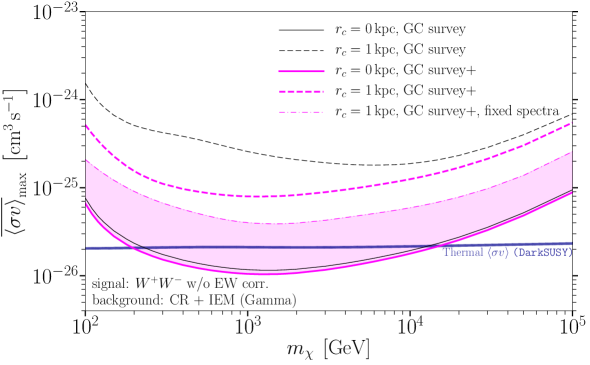
Figure 7: CTA sensitivity to a DM signal, for the $W^{+}W^{-}$ channel, comparing the case of an Einasto profile without core (solid) to that of an Einasto profile with a 1 kpc core (dashed). Black lines show the sensitivity with the base survey only and magenta lines show the sensitivity from adding extended survey observations. Modelling the spectral information with greater care may lead to a further improvement of the sensitivity to a cored profile, as indicated by the magenta dash-dotted line (see text for more details, including a discussion of the shaded area). In order avoid excessive use of computational resources, the sensitivity predictions in this figure are based on only 20 (equally log-spaced) energy bins.

In Fig. 7 we show how our limits for the $W^{+}W^{-}$ channel for the baseline Einasto profile (black solid line) worsen by about one order of magnitude when assuming large core sizes (black dashed line). The planned extended GC survey would clearly help to better distinguish even such an extended DM signal and would hence significantly improve limits in this case (magenta dashed line). For the Einasto profile (solid magenta line), on the other hand, the effect is minimal; here, the template discrimination is already so good for the standard survey that it is only the (slight) increase in observation time that implies a corresponding improvement. As discussed in Appendix C.2, additional spectral information can help significantly in the presence of large cores (but not for our benchmark case of a cuspy profile). With the thin dash-dotted magenta line, we indicate the maximal further improvement of limits that could be achieved this way (mimicking the situation where the astrophysical background components are well determined by complementary measurements; see Appendix C.2 for details). The magenta band can thus be interpreted as a rough estimate of how much our default projected DM limits could realistically be affected if the DM density profile turns out to be significantly less peaked than in the standard Einasto case. For similar reasons, we refrain from providing the full binned likelihood as in section 5.2: unlike in the case of cuspy profiles the normalisation given in Eq. (5.2) now depends on an effective $J$-factor that is itself energy-dependent (because the size of the region with highest SNR is energy-dependent, see discussion above), which in turn makes the translation to different density profiles and spectral shapes much less straight-forward.

We conclude that a large core in the DM distribution would indeed worsen the CTA sensitivity to DM annihilation – but much less severely than naively expected (or indicated by previous studies). This implies that, for DM masses in the TeV range, many models of thermally produced DM could be probed even in this highly unfavourable situation (both because of the statistical scatter in the expected mean limit, and because annihilation rates exceeding the ‘thermal’ rate by a factor of a few are by no means unusual, for example in the context of simple supersymmetric models [187, 188]). It is also worth stressing again that Fig. 7 summarises our assessment of what could be coined a ‘realistic worst-case scenario’; in reality, the situation can also be significantly better than the benchmark case of an Einasto profile, because of DM density spikes very close to the GC (see again Appendix C.2 for examples).

6 Discussion

In this section we turn to a discussion of our main results and how the projected sensitivities depend on the benchmark choices that we have adopted for our analysis. As stressed previously, one of the biggest challenges in the template fitting approach is a realistic account of systematic uncertainties both in the performance of the instrument and in the modelling of the templates. The parameters crucial to the description of the relevant physical effects are not only the magnitude of the systematic uncertainty, but also the correlation lengths, both in morphology and energy. Correlation matrices are an adequate way to describe these effects, as detailed in Section 4. We start by discussing instrumental systematic errors (related to the event reconstruction and hence mostly caused by misidentified CRs), which tend to dominate over astrophysical uncertainties (to be further discussed in section 6.2). While the importance of instrumental systematic uncertainties is already clearly seen in the right panel of Fig. 5, we note that they are potentially easier to study in real data (e.g. by defining special high-quality photon event classes).

6.1 Instrumental systematic uncertainties

In Fig. 8 we consider the impact of changing the overall spatial correlation lengths $\ell_{S}$ on our limits. Here we keep the overall systematic error amplitude to a fixed level of $\sigma_{S}^{\mathrm{instr}}=1$%, corresponding to our benchmark choice. Compared to our benchmark correlation length of $\ell_{S}=0.1^{\circ}$, corresponding to the typical PSF, limits worsen by a factor of up to three at intermediate DM masses, when $\ell_{S}$ is comparable to the spatial extension of the DM signal ($\lesssim 1^{\circ}$ for the Einasto DM profile). When signal and correlation lengths are sufficiently different, on the other hand, $\ell_{S}\lesssim 0.1^{\circ}$ or $\ell_{S}\gtrsim 1^{\circ}$, the impact of varying the correlation length on the sensitivity is generally milder – though the limit of very large correlation lengths would correspond to fixing the overall amplitude and hence result in the ‘statistical’ limit (with no systematic uncertainty in the spatial templates) indicated with a dashed line. Performing a similar exercise to explore the effect of energy correlations shows that these have a significantly weaker impact on the sensitivity to a DM signal, for our benchmark case of cuspy DM density profiles (but see Appendix C.2 for a discussion of how this changes in the presence of cores).

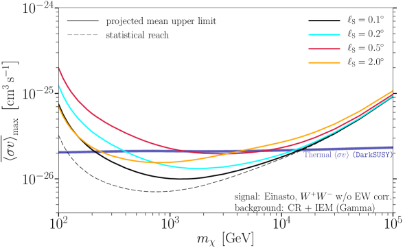
Figure 8: Solid lines show how the projected CTA sensitivity to a DM annihilation signal, for the $W^{+}W^{-}$ channel, varies with the spatial correlation length $\ell_{S}$, when keeping the instrumental systematic error-related fluctuation amplitude to a fixed level of $\sigma_{S}^{\mathrm{instr}}=1$%. For comparison, the dashed line show the statistical reach.

While our benchmark choice to account for systematic uncertainties may appear reasonable from the point of view of the expected instrument performance, we stress that this choice is not unique and other values of both $\sigma$ and $\ell$ may turn out to characterise the instrument more accurately. On the other hand, our benchmark scenario is by no means a carefully selected singular point, either, in the sense that various combinations of parameters would lead to similar conclusions. In fact, we can turn the problem around and ask for the required level of systematic errors allowing CTA to probe the thermal cross-section for standard assumptions about the DM profile. This question is explored in Fig. 9. In the left panel, we fix the DM mass to $m_{\chi}=2$ TeV and show the combinations of amplitude and spatial correlation length for which the thermal cross-section can be reached (green shaded area), while in the right panel we fix the fluctuation amplitude $\sigma_{S}$ and vary the correlation length and DM mass. The figure illustrates, as already seen in the discussion of Fig. 8, that one wants to avoid values of $\ell_{s}$ comparable in extension to the DM signal. In particular, for the design goal of $\sigma_{S}=1\%$, it is indeed crucial that the spatial correlation in mis-reconstructed events does not significantly exceed (a few times) $\ell_{S}\sim 0.1^{\circ}$. If the overall systematic uncertainty can be improved to be less than $1\%$, on the other hand, larger spatial correlations could be accepted.

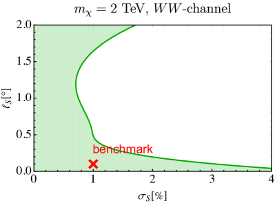
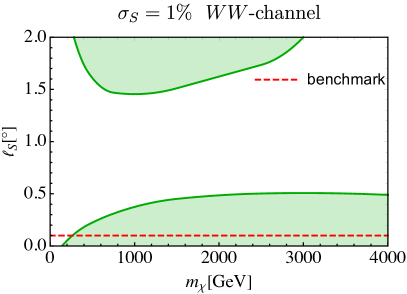
Figure 9: Contour plot (in green) showing the requirement on the instrumental systematic errors for which CTA is expected to reach the thermal cross section sensitivity to DM as a function of the amplitude and spatial correlation length of the instrumental systematic errors. For comparison, we mark the systematic benchmark settings used per default in this work (red cross in the left panel and dashed red line in the right panel). Left. For fixed DM mass $m_{\chi}=2$ TeV. Right. For a fixed overall systematic error amplitude of $\sigma^{\mathrm{instr}}_{S}=1\%$.

In the last part of this section we briefly comment on the impact of a set of internal (i.e. not yet publicly available) IRFs, based on tighter cuts for gamma/hadron separation and optimised for extended source detections (unlike the standard IRFs, which are optimised for point source detection). We checked explicitly that even with such optimised event cuts it will be hard to improve upon the sensitivity based on our standard IRFs. This can be understood by noting that, in the energy range where the DM sensitivity is best (few 100 GeV – few TeV), the misidentified CR background is already electron dominated, see Fig. 4, and it cannot be reduced significantly with current event reconstruction techniques. At the lowest and highest energies on the other hand, the tighter cuts can in principle substantially reduce the background, but only at the cost of reducing the effective area. We note, however, that these optimised IRFs still use the same event reconstruction scheme as the standard ones, so if an improved reconstruction algorithm becomes available in the future (benefitting from e.g. deep learning [189]) one may hope for more significant improvements.

6.2 Uncertainties in astrophysical components

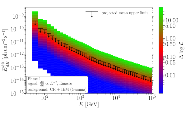
Figure 10: Differential flux sensitivity (time $E^{2}$) per energy bin to various gamma-ray templates in the GC region, corresponding to $2\sigma$ upper limits on mock data sets based on the residual CR background alone. The point source (PS) limit shows the statistical reach, for better comparison with published results, while the IEM and DM sensitivities adopt our benchmark scheme for the treatment of systematic errors ($\ell_{\textrm{S}}=0.1^{\circ}$, $\sigma_{\textrm{S}}=1\%$). For definiteness, we choose here a DM model with mass $m_{\chi}=100$ TeV annihilating to bottom quarks and the IE Gamma model (the dashed line show the emission intensity of the latter).

For the DM sensitivity targeted at by CTA, the astrophysical backgrounds discussed in Section 3 will have a stronger impact than for current generation instruments. In this section we aim to assess the associated uncertainties. For comparison, to set the scale, let us start by directly comparing the bin-by-bin integrated energy-flux sensitivities for different emission templates; this is done in Fig. 10, for mock data produced from the CR background alone. As expected, the sensitivity to the IE component (red) is significantly better than the flux expected in the Gamma model (dotted red line) – implying that it is indeed very likely that CTA will perform detailed measurements of this component. In comparison, the sensitivity to the DM template (blue) is worse by a factor of about two, related to the fact that the morphology of the IEM (elongated along the Galactic plane and following that of the gas column density) is less degenerate with the (much more isotropic) background of misconstructed CRs than the spherical DM signal. We checked explicitly that masking the Galactic ridge by excluding the region ($-1.5^{\circ}<l<1.9^{\circ},-0.5^{\circ}<b<0.5^{\circ}$) from the analysis does not change the relative sensitivity to the DM and IE component, which confirms that the difference is indeed related to the large-scale diffuse emission. For comparison, we indicate in the same figure also the flux sensitivity to point sources (green) obtained with our binned likelihood approach, which agrees very well with the official CTA point-source sensitivity based on an ON/OFF technique.

IE template uncertainty

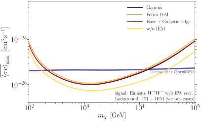
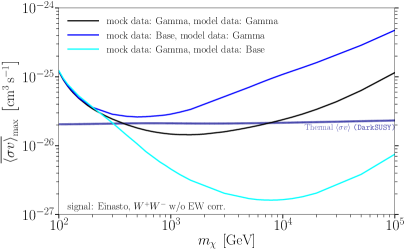
Figure 11: Left: CTA sensitivity to the DM annihilation channel for cases with no IE (yellow line) and with different IE models discussed in the text (note that the red line, for the Base IEM, largely overlaps with the black line, for our benchmark Gamma IEM). Right: Illustration of the projected DM sensitivity that would result from purposefully choosing a wrong IE model, compared to the one used in producing the mock data (sensitivities after adopting a Galactic plane mask of $-6.0^{\circ}<l<6.0^{\circ},-0.6^{\circ}<b<0.6^{\circ}$). Note that the large variation of limits shown here illustrates an extreme case, unrealistic to be encountered in the analysis of real data (see text for a discussion).

Let us now discuss in more detail how the modelling of the IE component affects the DM sensitivity. We start by exchanging our benchmark Gamma model for the alternatives mentioned in Section 4. The result is shown in Fig. 11 (left panel), for the Base (red) and Pass8-Fermi (orange) models. Adding IE thus degrades the DM sensitivity by almost a factor of two (black line). On the other hand, the effect of choosing IEMs more degenerate with the DM template (the Gamma model) or less ‘structured’ emission models (the Base model) is marginal. The apparent conclusion that the impact of varying the IE emission only mildly affects the sensitivity, however, is clearly overly optimistic because it implicitly relies on having access to the true emission model (modulo instrumental systematic uncertainties) when analysing the real data-set.

In the right panel of the same figure, we therefore relax this assumption and explore a different extreme, a pessimistic case, in which we purposefully chose a ‘wrong’ IE model with respect to the one used to produce the mock data (here we also use a Galactic plane mask, $-6.0^{\circ}<l<6.0^{\circ},-0.6^{\circ}<b<0.6^{\circ}$, since we do not attempt any IE modelling; masking however has limited impact on the IEM uncertainty, given that the differences extend beyond the plane). As illustrated, the limits could in this case artificially improve or worsen significantly more, by a factor of up to one order of magnitude. Let us stress that this plot is only meant to serve as an illustration, deliberately using two extreme IE modelling scenarios, neither of which is optimised for our energy range and ROI. With real data at hand, one would inspect the residuals to judge the quality of the fit and immediately discard models that deviate so significantly from the data as in the cases shown in this figure. In general, any residuals correlating with the galactic plane would strongly suggest that the IE modelling needs to be improved (and that DM limits obtained in this case are not realistic). Also the understanding of the IE itself is clearly expected to improve once real data are available. It is worth pointing out, however, that the issue of mis-modelling background components, as explored in this figure, could rather easily lead to fake signal claims and is hence much more relevant when assessing the DM discovery potential (rather than the potential to constrain a signal).

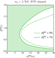
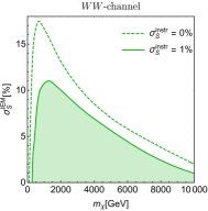
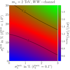
Figure 12: Left: The maximal uncertainty in the GDE template that can be tolerated for CTA to reach the ‘thermal’ cross-section sensitivity, as a function of the amplitude and spatial correlation length of the IEM systematic errors, for fixed levels of overall instrumental systematic errors of $\sigma_{S}^{\textrm{instr}}=1$% (solid line) and $\sigma_{S}^{\textrm{instr}}=0$% (dashed line). Middle: The maximal uncertainty in the overall IEM systematic error for CTA to reach the ‘thermal’ cross-section sensitivity, as a function of the DM mass, for $\sigma_{S}^{\textrm{instr}}=1$% (solid line) and $\sigma_{S}^{\textrm{instr}}=0$% (dashed line). Right: Mutual impact of instrumental and GDE model systematic uncertainties on DM limits (for the annihilation channel $\chi\chi\rightarrow W^{+}W^{-}$, at fixed DM $m_{\chi}=2$ TeV and for an Einasto profile), fixing $\ell_{\rm S}^{\rm instr.}=0.1^{\circ}$ and $\ell_{\rm S}^{\rm GDE}=1.0^{\circ}$. The colour scheme visualises the upper limit on the annihilation cross-section in units of the thermal annihilation cross-section for a given set of fluctuation amplitudes $\left(\sigma_{\rm S}^{\rm instr.},\sigma_{\rm S}^{\rm GDE}\right)$ in percent.

A different approach, more in line with our general treatment of systematic uncertainty, is to parameterise the GDE uncertainties via the correlation matrix. In Figure 12 we define the part of the parameter space $l_{s}^{\rm GDE}$ vs. $\sigma_{s}^{\rm GDE}$ for the GDE uncertainty for which we can reach the thermal cross-section (shown in green). In the left panel of that figure we focus on a fixed DM mass of 2 TeV, in two limiting cases where the instrumental systematic uncertainty $\sigma_{S}^{\textrm{instr}}$ is negligible (dashed lines) or corresponds to our benchmark-setting (solid lines). This figure demonstrates that, realistically speaking, it will be very challenging to reach the thermal cross-section if the GDE uncertainty significantly exceeds $\sim$5 - 10 %, at least for correlation lengths comparable to the DM signal shape (roughly $0.2^{\circ}-1^{\circ}$). To put this into perspective, we stress that template analyses based on Fermi-LAT data have already successfully been used to identify new emission components at the level of $\sim 10\%$ of the data, for example the Galactic Center Excess and the Fermi Bubbles [153]. One of the main ‘tools’ to identify new emission components or inadequate modelling is to inspect fit residuals, guiding model improvement in an iterative procedure. We envision that a similar approach will be possible also with CTA data. In the middle panel of that figure, we show that an even better understanding of the GDE component at the few-percent level is needed for DM masses both significantly below and above around 1 TeV.

In the above discussion, we have mostly emphasised whether the specific value of the ‘thermal’ cross-section can be reached. On the other hand, even for many thermally produced DM candidates, one expects annihilation rates that can easily be a factor of a few above this value. We, therefore, present a complementary view of the above considerations by showing, in the right panel of Fig. 12, the cross-section that can be probed in the $\sigma_{S}^{\textrm{GDE}}$ vs. $\sigma_{S}^{\textrm{instr}}$ plane for a given choice of the spatial correlation lengths ($l_{S}^{\textrm{GDE}}=1^{\circ}$, $l_{S}^{\textrm{instr}}=0.1^{\circ}$). As the figure shows, CTA will be able to probe models with only slightly enhanced annihilation rates even in the presence of instrumental systematic errors exceeding the current design goal and GDE uncertainties as large as $30\%$ (and more). Let us briefly mention that the above discussion is also closely related to that of applying a mask, which is the traditional choice of limiting the impact of such uncertainties. We take a more detailed look at this in Appendix B.3, concluding that for a template analysis the benefit of masking is at best unclear given that uncertainties in the GDE component are distributed across the entire ROI.

Localised sources and Fermi bubbles

Apart from the cosmic-ray induced interstellar emission, we expect two further contributions in our ROI, namely those connected to the low-latitude end of the Fermi bubbles as well as sub- and above-threshold sources. Here we briefly investigate how uncertainties in these components affect our DM limits.

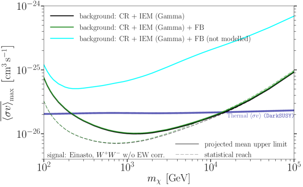
Figure 13: CTA sensitivity to a DM signal for our standard analysis settings (black solid line, as in Fig. 5), after adding an FB template (green solid line, largely overlapping with the black solid line) and the result of an analysis where the FB emission is present in the mock data, but not accounted for in the fitting procedure (cyan solid line). Dashed lines show the ‘statistical’ reach (neglecting systematic uncertainties in the spatial templates) for the former two cases.

Fermi Bubbles: In Fig. 13 we show the impact of adding the FB template to our benchmark set-up. As anticipated, this impact is rather limited because there is almost no degeneracy between the symmetrical DM and the off-centre FB templates. We remark, however, that if the FB emission (and in particular its morphology) turns out to be significantly different at CTA energies compared to the extrapolation based on the Fermi-LAT data, the impact of this emission component might be higher. To illustrate this, we indicate in the figure the limiting case where the FBs are left completely unmodelled; for TeV DM, this would (artificially) worsen the DM sensitivity by up to an order of magnitude. Studying this effect in more detail, which would involve studying the systematic uncertainties related to the physics modelling of the FBs, is beyond the scope of this work.

Non-diffuse sources: Concerning the emission from bright (resolved) localised sources, our baseline procedure is to mask them in order to limit their impact on the fitting procedure. While such a procedure works well with mock data, it was realised already with the Fermi-LAT analysis that masking in crowded regions poses several challenges related to the choice of a proper mask size and the modelling of the source emission that ‘leaks’ outside the mask. Besides, cumulative emission from sub-threshold sources could result in a significant diffuse emission component that is challenging to model. A detailed treatment of these issues is also beyond the scope of this work. Here we instead limit ourselves to verifying that leakage of sources, for the current five bright sources we consider, affects the limits by roughly $30\%$ (when we mask sources with a $0.1^{\circ}$ mask, while the emission effectively extends out to approximately $0.5^{\circ}$ for lower energies). We further checked explicitly that sub-threshold sources will not affect the DM sensitivity with respect to the benchmark scenario as long as this contribution is modelled ‘perfectly’, c.f. Fig. 11 (left panel) for a similar conclusion regarding IE models. In the most pessimistic case on the other hand, where such a component is present in the data but left unmodelled, the impact on the DM sensitivity can reach up to a factor of a few; unlike in the case explored in Fig. 11 (right panel), we note that this typically results in an artificial strengthening of the projected DM constraints, as the IE model overcompensates for the sub-threshold emission. We note however that, similar to the case of IEM, the potential impact of mis-modelling this component is likely much higher in the case of the detection of a potential DM signal.

7 Summary

The CTA observatory will have excellent charged particle discrimination, an improved angular resolution, a wide energy coverage and a larger effective area than currently operating atmospheric Cherenkov telescopes, making it a promising instrument to detect large-scale gamma-ray emission. All these attributes of CTA are also highly relevant for DM searches, motivating the expectation that CTA will significantly improve upon the DM sensitivity of existing IACTs and possibly make a major discovery. Indeed, probing a potential signal from annihilating DM has long been stated as one of the primary scientific goals of CTA which is soon entering the construction phase.

This article represents the most detailed assessment of the CTA sensitivity to DM signals at the GC so far, taking into account details of the planned observational strategy of that region and the latest IRF versions. We also use state-of-the-art modelling of the emission components in this region, including interstellar emission (IE), known and unknown (subthreshold) sources and Fermi bubbles, based on currently available measurements coming mainly from Fermi-LAT and H.E.S.S. data.

From the perspective of fundamental physics, our most important finding is the confirmation that CTA will be able to reach the ‘thermal’ cross-section for TeV-scale DM, a milestone for probing the WIMP paradigm at these masses, for a large range of well-motivated assumptions about the instrument’s performance; Figs. 9 and 12 present a new and refined way of presenting these conclusions. In particular, these figures quantify the level to which the instrumental systematic errors need to be controlled if CTA is to achieve its designated goal of testing the ‘thermal’ annihilation cross-section of DM. We also find that the existence of a cored DM distribution would clearly deteriorate CTA’s sensitivity to a DM signal – but only by a factor of a few, c.f. Fig. 7, i.e. significantly less than expected from earlier studies adopting smaller ROIs. While the ‘thermal’ cross-section would likely (just) be missed in that case, it is important to stress that there is still a plethora of well-motivated particle physics models predicting DM candidates which would leave a sizeable gamma-ray signal in CTA data even in this case (for example in the context of simple supersymmetric models [187, 188]).

In arriving at the above conclusions, a major motivation of our work was also to explore the most promising data analysis procedures. We therefore confronted the traditional ON/OFF analysis technique with a template fitting analysis procedure, still not yet widely explored by IACT collaborations. In Appendix C.4 we demonstrate that for the set of Fermi-LAT inspired IE models and given the CTA sensitivity, this technique leads to a decidedly better performance. As is typical for template fitting procedures, the main source of uncertainty lies in the systematic errors originating from the event classification and/or the modelling of the emission components. We include such systematic errors directly in the likelihood, in a parametric way, thereby accounting for their spatial and energy correlations (sections 6.1 and 6.2). Ideally, the output of such an ‘agnostic’ approach to studying the impact of instrumental systematic errors can be used for future IRF optimisation once CTA is fully operational.

It is worth stressing that the relative impact of the various sources of uncertainties on the DM sensitivity was difficult to judge prior to this study. For example, CTA is expected to greatly advance the measurement of large-scale interstellar emission at TeV energies, thus effectively identifying an additional background component and thereby potentially lowering the constraining power of CTA to a DM signal (compared to the situation where such a background would not be present). An important result of our analysis is that the impact of this large-scale diffuse component is rather limited, as long as the associated modelling uncertainties are not very large ($\sigma_{S}^{\rm IE}\lesssim 10\%$). While a smaller value of $\sigma_{S}^{\rm IE}$ presently appears rather optimistic given the best existing models, it is expected to become a realistic assumption once the IE models can be tuned to actual CTA measurements. In that case instrumental systematic uncertainties will continue to play the dominant role in constraining a signal. For larger uncertainties in the IE component on the other hand, the impact on the DM sensitivity can be comparable to that from purely instrumental effects.

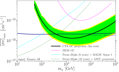
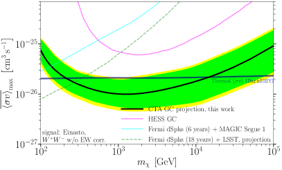
Figure 14: The CTA sensitivity curves derived in this work (black line, see Fig. 5) for the $b{\bar{b}}$ (l͡eft) and $W^{+}W^{-}$ (right) channels, shown together with the current limits from Fermi-LAT observation of dSph galaxies (cyan) [177] and H.E.S.S. observations of the GC (purple) [165]. In addition we show the projection [190] of the Fermi-LAT sensitivity where future dSphs discoveries with LSST are taken into account (dashed green). Note that the projected sensitivity of CTA shown here includes our estimate of systematic uncertainties (1% overall normalisation error and a spatial correlation length of $0.1^{\circ}$); for the corresponding results for the initial construction configuration of CTA, see Appendix A.

Sub-threshold sources could turn out to be an additional important source of systematics, though based on the current study their impact appears to be more limited. We also included templates for the Fermi bubbles in our analysis, finding that their impact on DM limits is generally subdominant compared to that of the IE (Section 6.2). This conclusion rests on the assumption that the underlying models are sufficiently reliable, a hypothesis that strictly speaking will only be possible to test with sufficient accuracy once actual data are present. While we do not expect major impacts on the expected limit on a DM signal that CTA will be able to put, the impact of modelling uncertainties in these components on a potential signal claim would likely be much larger. Compared to the case of the IE template, which can be improved with input from complementary observations, it may not be straight-forward to reduce the effects of sub-threshold sources or the Fermi bubbles. In that case, these emission components would potentially present an irreducible background that would prevent a robust DM discovery.

To provide a somewhat broader perspective, we conclude by comparing, in Fig. 14, the CTA sensitivity derived in this work to current (and, for the case of Fermi-LAT, projected) DM limits from complementary observations. Noting that the CTA sensitivity projections take into account instrumental systematic uncertainties, this figure nicely illustrates how CTA will improve on the pioneering work of the current generation of IACTs to test WIMP DM, and to significantly extend the range of DM masses where we can robustly probe the theoretically important benchmark that is provided by the thermal annihilation rate. In that sense CTA will indeed provide a unique opportunity to test the WIMP paradigm, in particular when keeping in mind that even annihilation rates a factor of a few larger than the ‘thermal’ annihilation rate are not uncommon among proposed models to explain the particle nature of DM. In Appendix A we demonstrate that much of the discovery space remains available even for the reduced observational programme associated with the initial construction configuration of CTA – though of course the baseline array considered in the main text will clearly probe more of the critical parameter space and hence have a significantly better leverage to test the WIMP hypothesis. For either of these scenarios we believe that the chance to obtain unique clues about the nature of DM, newly assessed and confirmed here, makes this part of CTA’s science programme truly imperative.

Appendix A Initial construction configuration

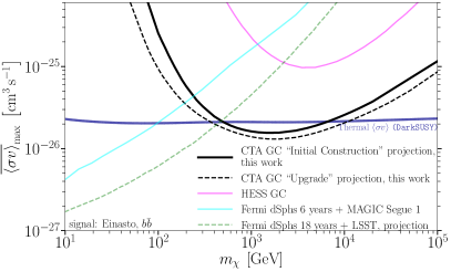
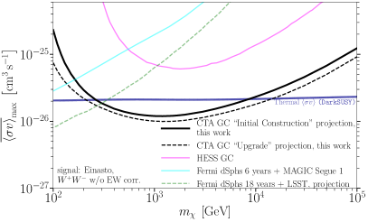
Figure 15: Same as Fig. 14, but the solid black line now shows the sensitivity projection for the reduced initial construction configuration (while the dashed black line shows the result for the benchmark analysis setting presented in the main text).

Given the substantial investment in infrastructure that is required for an instrument with the size of CTA, it is not surprising that current planning calls for the telescope arrays to be constructed in phases. In the main text we have discussed the ‘baseline array’, i.e. the array configuration corresponding to the original design goal. In this Appendix we instead consider a slimmed-down (initial) construction configuration and discuss the impact of this preliminary configuration on CTA’s sensitivity to a DM signal and its ability to test the WIMP paradigm. It is worth stressing that the construction configuration could be realised with the funding that is currently available at the time of this writing.

The reduced South array we considered is composed of 15 MSTs, 50 SSTs and no LST, which compares to a baseline South array of 4 LSTs, 25 MSTs and 70 SSTs that was considered in the main text. Here we follow exactly the same analysis steps as described in the main text, in particular concerning the treatment of systematic errors, but generate templates and mock data based on IRFs describing this initial configuration instead.

In Fig. 15 we illustrate the projected sensitivity for this array configuration (black solid lines) in analogy to Fig. 14 in the main text, including for convenience also the sensitivity for the full baseline array derived there (black dashed lines). The loss in sensitivity of the reduced array is clearly visible and can, for DM masses above 200 GeV, mainly be attributed to the reduction in the number of MSTs; for smaller DM masses the lack of LSTs leads to a further clearly visible decrease in sensitivity (see also Appendix C.3). When only focussing on this direct comparison between the two array layouts, the difference between the two configurations may still not appear very dramatic. However, in comparison to expected results from complementary techniques, in particular the projected limits from Fermi LAT, it becomes clear that this impression is misleading. While there are many WIMP realisations somewhat above the ‘thermal’ line, the number increases substantially as one gets close to the line (and slightly below it). Losing the opportunity to robustly exclude annihilation cross-sections within a factor of a few around this ’thermal’ value thus results in a significant loss in theoretical models that can be probed, correspondingly diminishing the prospects for the detection of thermally produced DM. Accordingly, it remains a critical goal to eventually reach the baseline CTA configuration that is discussed in the main text.

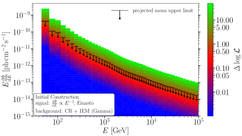
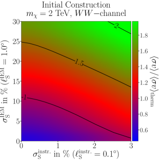
Figure 16: Left. Differential flux (times $E$) as a function of source energy $E$, with the (logarithmic) colour scale indicating the change in the total likelihood due to the contribution from a DM signal in the respective energy bin. Same as Fig. 6, but with respect to the initial construction configuration of the array. Also in this case the full likelihood table is available for download at zenodo [178]. Right. Mutual impact of instrumental and GDE model systematic uncertainties on the upper limit on the DM annihilation cross-section. As in Fig. 12 (right panel), but now with respect to the construction configuration.

As discussed in section 5.2, directly providing the bin-to-bin flux sensitivity to DM signals in general allows one to test DM annihilation in the most model-independent way, in particular for models where the annihilation spectra deviate from those expected for pure annihilation channels like $\bar{b}b$ or $W^{+}W^{-}$. In Fig. 16 (left panel) we show this binned likelihood for the construction configuration; in particular, this allows us to use Eq. (5.1) to calculate limits in the same straightforward way as before. Just as for the baseline configuration, we make this likelihood available in tabulated form in the supplemental material.

We conclude our discussion of the initial CTA configuration by showing, in the right panel of Fig. 16, the required level of instrumental systematic uncertainties and modelling uncertainty in the IE component to reach the thermal cross-section. This should be directly compared to Fig. 12 in the main text. As expected, a somewhat better control of instrumental systematic uncertainties is needed to achieve the same performance goals as for the baseline array.

Appendix B Details of IE models

B.1 Spectral differences in the Galactic Ridge region

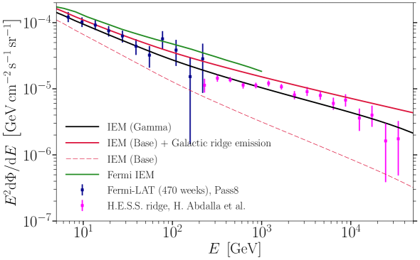
Figure 17: Differential $\gamma-$ray flux (times $E^{2}$) of the Galactic ridge region ($\left|b\right|\leq 0.3^{\circ}$, $\left|l\right|\leq 1.0^{\circ}$) as measured by H.E.S.S. [137] (magenta) and Fermi-LAT (blue) [191]. We also show three IE/GDE models as described in Section 3.2: two phenomenological models [144], Gamma (black) and Base + Galactic ridge (red), and a data-driven Pass8 Fermi-LAT diffuse model (green).

In Fig. 4 in the main text we compared the expected photon counts resulting from our emission components (including all three IE/GDE models that we use) integrated over the full ROI. At TeV energies there are a few existing measurements of a diffuse component that, e.g. , have been performed by the H.E.S.S. collaboration [136, 137] or the VERITAS collaboration [138, 192], albeit mostly restricted to the Galactic Ridge region. Here we mostly refer to the published results by H.E.S.S. and in Fig. 17, we therefore complement Fig. 4 by showing how the three IE/GDE models compare to these data in this significantly smaller region.

Concretely, we plot the flux inside this region as expected from the Gamma model (black) and the data-driven Pass8 Fermi-LAT diffuse model (green). As already pointed out in the main text, the construction of the Base model (red dashed) does not explicitly account for the TeV emission from the Galactic Ridge; we therefore add to this model (red solid) a spatial template for the Galactic ridge adopted from Ref. [136], with a spectrum modelled as a power-law with spectral index $\gamma=-2.28$ [137] and normalised to the H.E.S.S. measurement. For comparison we also show in this figure data points from Fermi-LAT (blue) and H.E.S.S. (magenta). The former are adopted from Ref. [191] and represent 470 weeks of Pass8 data after subtracting the emission of known point sources from the 3FGL catalogue. Neither of these data sets has the isotropic emission component subtracted, which however is negligible compared to the expected IEM in this region.

We conclude that all three models are in reasonable agreement with the data in this region, and are therefore also reasonable to use at small scales.

B.2 Morphological differences

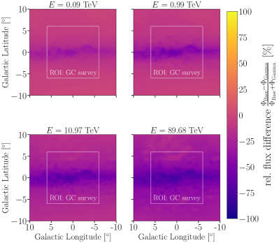
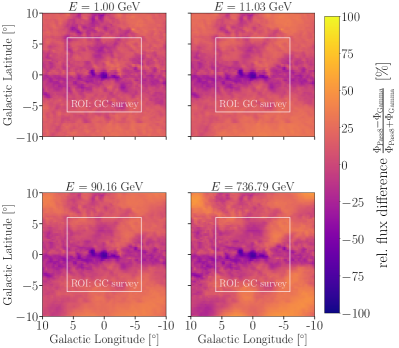
Figure 18: Left. Relative flux difference between the Gamma and Base IEMs, the square marking our ROI. Right. Same, but for Gamma and Pass8 Fermi-LAT IEMs.

As described in the main text, our three benchmark IE models are chosen to represent a fully complementary approach to modelling the GC region. Here, we further explore these models by investigating morphological differences between them.

The Gamma and Base models, in particular, are produced using the same numerical code, DRAGON [193], based on the same target gas and ISRF distribution (and identical to that given in version v.54 of the GALPROP code [194]), so the only difference consists in how CR diffusion is treated. In the left panel of Fig. 18 we show the normalised difference between the expected flux for these models, spatially resolved in the GC region and for four selected values of the gamma-ray energy between about 100 GeV and 100 TeV. This difference is, as expected, largest in the central regions, at a level of up to about $60\%$; even at the outskirts of our ROI, however, the differences can be larger than $20\%$, especially at higher energies. We note that these numbers should be roughly compared to the parameter $\sigma_{S}^{\rm IEM}$ that we discuss in section 6.2 of the main text.

In the right panel of Fig. 18 we perform the same comparison, but for the flux ratio between the Gamma and Fermi-LAT Pass 8 GDE models, where the latter now is based on different gas maps. A qualitative difference in this case is that the residuals can be both positive and negative. The negative residuals displayed here mainly coincide with the location of interstellar clouds.

B.3 Effect of masking

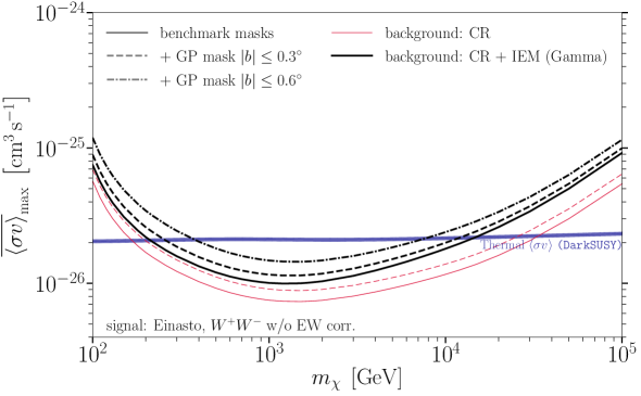
Figure 19: CTA sensitivity to a DM signal, and how it is affected by masking the Galactic plane. Solid lines indicate the result when not applying any masks (beyond those for the extended sources shown in the top left panel of Fig. 3), and dashed (dash-dotted) lines indicate the result of implementing additional masks with $\left|b\right|\leq 0.3^{\circ}$ ($\left|b\right|\leq 0.6^{\circ}$). Black lines assume the standard CR and IEM background, while purple lines assume instrumental (CR) backgrounds alone. The thick solid line is thus identical to one in the left panel of Fig. 5, showing the CTA DM sensitivity as obtained in our benchmark analysis setting.

The discussion of the GDE modelling uncertainty is closely related to the choice of the masking, which is traditionally used to limit its impact on DM searches. In Fig. 19 we plot the change in the DM sensitivity caused by masking, assuming that we mask the whole galactic plane (GP) out to latitudes of $|b|<0.3^{\circ}$ and $|b|<0.6^{\circ}$, respectively. We see that masking has a rather limited effect when GDE is accounted for (both in the data and in modelling), as shown by the thick lines; in contrast, the decrease in sensitivity is more pronounced in the absence of a GDE component (thin lines).

This is consistent with our Signal-to-Noise Ratio (SNR) studies (Appendix C.1) demonstrating that little information comes from the plane when a diffuse emission is present. We note that, while our limits can worsen by up to a factor of 2 (for 2 TeV DM, 30% IEM uncertainty and $0.5^{\circ}$ correlation length, c.f. Section 6.2), they worsen by only up to a factor of 1.5 when a $0.6^{\circ}$ region is masked. If all IE uncertainty was localised along the plane, masking would thus indeed be beneficial. However, as just illustrated in Appendix B.2, model differences (i.e. IEM systematic uncertainties) cover most of our ROI, making the masking approach challenging to implement. In practice, this demonstrates that once real data is available, a careful study of the GDE uncertainty will be needed and will guide the masking choices and/or interpretation of potential discovery hints.

Appendix C Further analysis details

C.1 Signal-to-Noise ratio and information flux

In this section, we study in more detail the SNR in our ROI, which is useful for understanding various aspects of the general discussion. At a technical level, we use swordfish [171] to calculate a generalisation of the SNR that also captures the effect of systematic errors, namely the so-called Fisher Information Flux $\mathfrak{F}$ [170]. In the statistics-dominated regime, by definition, $\mathfrak{F}$ becomes identical to SNR.

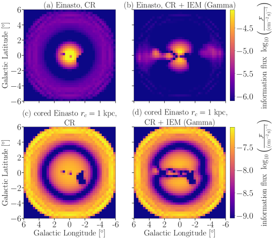
Figure 20: Left column: Information flux $\mathfrak{F}$ (logarithmic colour scale), for Einasto (upper panel) and cored DM profiles (lower panel), assuming only the misidentified CR background (and no IE). Right column: Same, but with the added emission based on the Gamma model. Regions with large $\mathfrak{F}$ yield most of the constraining power to a DM signal. These $\mathfrak{F}$ maps are based on the full GC survey, assuming our benchmark scheme of treating instrumental systematic uncertainties.

In the left column of Fig. 20 we show this quantity for the Einasto (upper panel) and a cored Einasto DM profile (lower panel), respectively, assuming only the background of misidentified CRs. The resulting $\mathfrak{F}$ is spherical, following as expected the signal shape. The blue ring-like feature indicates a sharp drop in $\mathfrak{F}$ that separates two regimes: i) a central region, containing information on the signal emission, and ii) the outer regions that provide constraining information on the CR background (which is much more isotropic than any of the other components). In this situation, most of the constraining power comes from the inner 0.5^∘ for an Einasto profile (which we have used in Section 6.1) and $\sim 1^{\circ}$ for a cored profile. Adding an IE component (right column) deforms the spherical region of large $\mathfrak{F}$ into an hourglass shape for cuspy profiles – which indeed is the general expectation for the optimal ROI shape in such a case [195]. However, sizeable excesses in $\mathfrak{F}$ also appear along the Galactic plane – though less pronounced than in the centre – with size and position depending on the chosen spatial correlation length $\ell_{\mathrm{S}}$; these excesses are related to regions where more observation time is necessary to break the relatively strong degeneracy between IE and DM templates. In comparison, fixing the exact normalisation of the CR template is less crucial, which explains the smaller amount of information to be gained from the edges of the ROI (as compared to the upper left panel of the figure). This situation changes somewhat for a cored profile, as shown in the bottom right panel, where the degeneracy between the IE and DM templates is less severe. As a consequence, spending observation time on the edges of the ROI is still profitable in terms of constraining power. The upper right panel of Fig. 20 provides a solid ground to argue why a Galactic plane mask with moderate size does not strongly affect the DM limits, cf. Fig 19. Especially for a mask of $\left|b\right|\leq 0.3^{\circ}$, the effect is rather mild since the maximal values of $\mathfrak{F}$ are concentrated in the upper and lower region of the hourglass outside of the mask.

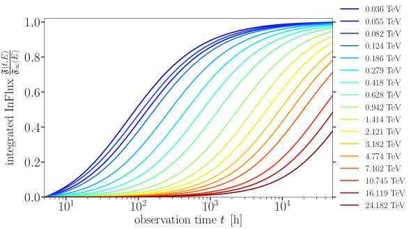
Figure 21: Time-integrated information flux $\mathfrak{F}(E,t)$ per energy $E$ as a function of observation time $t$, normalised to the maximally available integrated information flux $\mathfrak{F}_{\infty}(E)$. Here we assume a circular ROI of radius $2^{\circ}$ centred on the GC, an Einasto DM density profile, a generic DM annihilation spectrum $\Phi\propto E^{-2}$ and the Gamma IEM, adopting our benchmark scheme for treating instrumental systematic uncertainties. In order to avoid excessive use of computational resources, the sensitivity predictions in this figure are based on only 20 (equally log-spaced) energy bins.

In Fig. 21 we show instead how the time-integrated information flux evolves with the observation time, for different energy bins (quoted energy values correspond to the central energy of each bin). Here, for better comparison, we have (for each energy bin separately) normalised $\mathfrak{F}$ to the asymptotic value it would take after an ‘infinite’ observation time. The figure illustrates that most information at the lowest energies, for $E\lesssim 200$ GeV, is already extracted after around 100 h of observation time. Gaining a significant share of the in principle available information ($\gtrsim 0.5$ in this normalisation) at TeV energies, on the other hand, clearly requires observation times of at least 1000 h.

C.2 Different DM profiles and impact of energy correlations

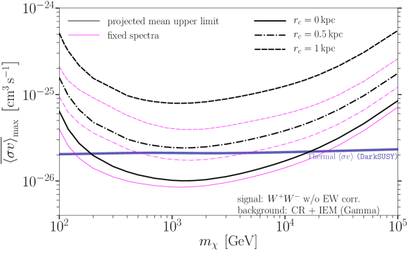
Figure 22: CTA sensitivity to a DM signal, for the $W^{+}W^{-}$ channel, for various choices of the DM profile. Solid lines show the case of an Einasto profile with no central core, while dashed (dash-dotted) lines show the case of an Einasto profile with a central core of radius 1 kpc (0.5 kpc). Black lines correspond to the result of our benchmark analysis setting, while magenta lines demonstrate the improvement of these limits when adding on top of the (spatial) instrumental systematic uncertainties a long-range correlation in energy, which effectively fixes the spectral shapes of the background components. For definiteness, we choose here an energy correlation length of $\ell_{\rm E}=8$ dex, and adopt overall normalisation uncertainties in the CR (IEM) component of $\sigma^{\rm instr.}_{\rm E}=1\%$ ($\sigma^{\rm IEM}_{\rm E}=10\%$). In order to avoid excessive use of computational resources, the sensitivity predictions in this figure are based on only 20 (equally log-spaced) energy bins.

For the distinct morphology of our benchmark (Einasto) DM profile, as stressed several times, uncertainties in the spectral information of the templates only play a sub-dominant role. This can, however, change in the presence of the cored profiles discussed in section 5.3, where adding spectral information can be expected to help in distinguishing the emission components, and thus to improve the DM sensitivity. A detailed study of how to potentially improve the modelling of background components is beyond the scope of this work, also because we do not yet have actual data to compare to, but in Fig. 22 we illustrate the expected effect in terms of systematic uncertainties associated with the spectral components. The black lines show our benchmark analysis setup, assuming no energy correlations, while the magenta lines show the effect of adding such correlations over a range larger than the whole energy window adopted in our analysis (thus effectively fixing the spectrum in the analysis). Solid, dashed and dotted lines refer, as in Fig. 7, to the DM density profile that is adopted. For the Einasto profile, the sensitivity to a DM signal improves by up to 40 % when taking into account the additional information contained in the assumed energy correlations. For a 1 kpc core, on the other hand, the improvement is much more significant and can be larger than a factor of 2.

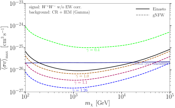
Figure 23: CTA sensitivity to a signal from DM annihilating to $W^{+}W^{-}$ for a gNFW DM density profile (dashed lines), for various choices of the slope parameter $\gamma$, as indicated (and corresponding best-fit values for scale radius $r_{s}$ and local DM density $\rho_{\odot}$ as derived in Ref. [84]). The solid black line shows, for comparison, the upper limit for our standard Einasto profile. All upper limits incorporate our benchmark scheme for the treatment of instrumental systematic uncertainties. We stress that the range of DM density profiles shown here does not include the possible enhancement of the DM density in the central ($r\ll 1$ kpc) regions of the Galaxy, which would further contribute to an increase of the CTA sensitivity. Possible spectral correlations (increasing the sensitivity for $\gamma\leq 1$ profiles) are also not considered here.

In the final part of this section we illustrate the uncertainty of the projected sensitivity due to the rather poorly constrained spatial profile of DM in the Galactic centre in a complementary way, this time assuming no energy correlations (and thus returning to our benchmark settings, for better comparison with the results of the main text). In Fig. 23 we show a summary of expected limits for exemplary parameter choices with respect to a generalised NFW (gNFW) DM density profile:

$$\rho_{{\rm gNFW}}\!\left(r\right)=\frac{\rho_{s}}{\left(\frac{r\vphantom{x_{s}^{2}}}{r_{s}}\right)^{\gamma}\left(1+\frac{r\vphantom{x_{s}^{2}}}{r_{s}}\right)^{3-\gamma}}{\rm.}$$ (C.1)

Our parameter choices are motivated by Fig. 4 of a recent Bayesian analysis of MW data [84]. In particular, we pick a range of values for $\gamma$, within $1\,\sigma$ of its best fit value, and then choose the corresponding best-fit values for the remaining two parameters, $\left(r_{s},\rho_{\odot}\right)$, which we collectively list in Tab. 1. Fig. 23 illustrates that NFW limits are somewhat more stringent than those obtained with our benchmark Einasto profile, and that the adopted range of $\gamma$ values results in sensitivities symmetric with respect to our benchmark case. Note that the sensitivities are calculated for the extended survey (which increases sensitivity for more cored profiles), but without spectral information (implying that the results shown for $\gamma=0.4$ are overly pessimistic). We stress that the most recent numerical simulations, when correlated with Gaia data of the baryonic content of the MW, tend to produce a DM profile that is steeper in the inner Galaxy than the Einasto case [98]. Furthermore, a possible enhancement of the DM density in the very central ($r\ll 1$ kpc) region of the Galaxy, e.g. due to the presence of the supermassive black hole [196, 197, 198], cannot presently be constrained by kinematic analyses like that of Ref. [84]. In conclusion, even smaller cross-sections than indicated in Fig. 23 can potentially be tested with CTA.

$\gamma$	$r_{s}\;\left[\mathrm{kpc}\right]$	$\rho_{\odot}\;\left[\mathrm{GeV}\,\mathrm{cm}^{-3}\right]$
0.4	6.7	0.44
1.0	10.7	0.43
1.1	11.7	0.43
1.26	13.2	0.43

Table 1: Summary of the gNFW profile parameters extracted from Fig. 4 of [84].

C.3 Individual contribution from different telescope types

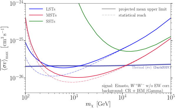
Figure 24: CTA sensitivity to a DM signal, independently derived for the three telescope types (LSTs – blue, MSTs – red, SSTs – green) according to the Southern Array layout, both for our standard analysis pipeline (solid) and when neglecting systematic uncertainties (dashed). Note that in the case of SSTs the solid and dashed (green) lines are overlapping.

In this section, we discuss how the three main telescope types individually contribute to the DM sensitivity. On the one hand, this potentially helps to assess how CTA’s sensitivity will improve during the first years of data taking, once the deployment schedule is set. On the other hand, the breakdown of telescope sensitivities with respect to the telescope types is clearly also relevant in view of potential upgrade steps following the initial configuration discussed in Appendix A.

In Fig. 24 we illustrate the DM sensitivity that results when only taking into account one type of telescopes, respectively, in the Southern array Baseline Configuration and adopting out benchmark treatment of systematic uncertainties (solid lines). For comparison, we also indicate the resulting limits in the case when no systematic uncertainties are explicitly added in the analysis (dashed lines). As expected, the LSTs dominate the sensitivity for the lowest DM masses accessible to CTA (below $\sim 100$ GeV). In the middle mass range the MSTs dominate, increasing the overall reach due to the larger number of telescopes (25 MSTs vs. 4 LSTs are planned for the Southern site). SSTs are most relevant for the highest energies, but their sensitivity only starts to be competitive for DM masses around 100 TeV. As clearly visible also when broken down to individual telescope types, limits are dominated by systematic errors for low DM masses/photon energies, and statistics-dominated for high DM masses/photon energies.

C.4 ON/OFF analysis

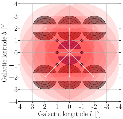
Figure 25: Schematic visualisation of the chosen ON (purple) and OFF (black) regions in the context of CTA’s Galactic centre survey. The choice of the latter is based on the six pointing positions with Galactic latitude $|b|=1^{\circ}$ (indicated by crosses), see text for details. The Galactic plane in the ON region is masked for $\left|b\right|\leq 0.3^{\circ}$, which is reflected in the definition of the OFF region(s) as well. Both ON and OFF regions are split into five concentric annuli of width $0.2^{\circ}$.

Here we briefly compare the performance of our default template fitting technique to the ON/OFF type of analysis discussed in Section 4. For the latter, we adopt a likelihood that is a product of Poisson likelihood functions $\mathcal{L}_{ij}$ over the $i-$th energy, $j-$th ON region (ring) and $k-$th pointing position (as used in, e.g., Ref. [186]):

$$\mathcal{L}\!\left(M_{\textrm{DM}},\langle\sigma v\rangle\right)= \prod_{ijk}\,\mathcal{L}_{ij}\!\left(\mathbf{N^{\textrm{S}}_{k}},\mathbf{N^{\textrm{B}}_{k}},\mathbf{\kappa_{k}}\left.\right|\mathbf{N^{\textrm{ON}}_{k}},\mathbf{N^{\textrm{OFF}}_{k}}\right)$$ (C.2)

$$= \prod_{ijk}\,\,\frac{\left(N^{\textrm{S}}_{ijk}\!\!+\!\!\kappa_{ijk}N^{\textrm{B}}_{ijk}\right)^{N^{\textrm{ON}}_{ijk}}}{N^{\textrm{ON}}_{ijk}!}e^{-(N^{\textrm{S}}_{ijk}+\kappa_{ijk}N^{\textrm{B}}_{ijk})}\times\frac{\left(N^{\textrm{B}}_{ijk}\right)^{N^{\textrm{OFF}}_{ijk}}}{N^{\textrm{OFF}}_{ijk}!}e^{-N^{\textrm{B}}_{ijk}}\,,$$

with $N^{\textrm{S}}_{ijk}$ denoting the expected number of signal events in the ON (‘signal’) region. $\mathbf{N_{k}}^{\textrm{ON}}$ and $\mathbf{N_{k}}^{\textrm{OFF}}$ refer to the measured photon events in ON and OFF region for observation $k$ which we prepare as a single Asimov data set from a selection of background source components described in Sec. 3.2. $\kappa_{ijk}$ is in general a normalisation factor to account for the different background acceptance in the ON and OFF regions, but in our case it will by construction be equal to one for all bins.

Fixing the value of $m_{\chi}$, we again choose the likelihood ratio as test statistic to constrain $\langle\sigma v\rangle$. To this end, we adopt Eq. (4.2) to our purposes here, by explicitly profiling over the nuisance parameters $N^{\textrm{B}}_{ijk}$; as a result, we obtain a one-dimensional likelihood function depending only on the signal strength $\langle\sigma v\rangle$. The definition of ON and OFF regions closely follows the scheme outlined in Ref. [186]. We define our ON region as a circular ROI of $1^{\circ}$ radius centred at the GC, divided into five concentric annuli with a width of $0.2^{\circ}$, and mask the region with $\left|b\right|\leq 0.3^{\circ}$ to remove the brightest very high-energy point sources in the vicinity of the GC and parts of the IEM. The position of the OFF regions is chosen as the point-symmetrical image of the ON region with respect to the respective observational pointing position (see Fig. 25), which, under the assumption of an instrument response that depends only on offset from the pointing direction but not azimuth, implies that ON and OFF regions share the same solid angle, exposure and acceptance. Fig. 2 in the main text illustrates that for cuspy DM density profiles the $J-$factors of ON and OFF region can differ by up to one order of magnitude so that the OFF region should indeed only feature minor contaminations by the signal source. Splitting the ON and OFF ROI into multiple annuli improves the performance of indirect DM searches following an ON/OFF analysis [165].

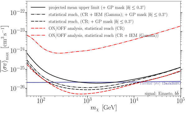
Figure 26: Mean expected CTA upper limits on the DM annihilation cross-section for the $\bar{b}b$-channel and an Einasto DM density profile, adopting the default morphology analysis (black) and ON/OFF strategy (red), respectively. The black solid line represents the benchmark situation (including instrumental systematic errors) where we additionally apply a mask to the band $b\leq 0.3^{\circ}$ to reduce the impact of the IEM along the Galactic plane. All other lines refer to ‘statistics-only’ limits, where the impact of systematic errors is neglected; dashed (dash-dotted) lines assume that no IE (IE as expected in the Gamma model) is included in the mock data. Note that in each of the cases shown here the Galactic plane is masked. In order to avoid excessive use of computational resources, the sensitivity predictions in this figure are based on only 20 (equally log-spaced) energy bins.

In Fig. 26 we compare expected limits from our benchmark analysis (black lines) with those resulting from the ON/OFF analysis as described above (red lines). The first crucial observation is that the two approaches result in a comparable sensitivity when only including the smoother background of misidentified CRs, and no IE, in the simulated data (dashed lines); this provides a nice consistency check of the two methods in the absence of extended diffuse emission components – which indeed is the basic assumption that previous DM searches with IACTs have relied on. Adding IE (our default Gamma model) to the simulated data, however, the ON/OFF analysis suffers as expected from a significant loss of sensitivity (red dash-dotted), while limits obtained from the morphology analysis (black dash-dotted) are much less affected. This illustrates, as already argued previously, that the ON/OFF analysis can only be expected to provide realistic DM limits if the expected large-scale diffuse emission components are either below the nominal sensitivity of the instrument, or exhibit a rather low gradient within the ROI. In all other cases, at least under the assumption that the spatial IEM templates can be modelled more or less realistically, the morphological analysis appears to be more promising.

CTA Acknowledgements

We gratefully acknowledge financial support from the following agencies and organisations:

State Committee of Science of Armenia, Armenia; The Australian Research Council, Astronomy Australia Ltd, The University of Adelaide, Australian National University, Monash University, The University of New South Wales, The University of Sydney, Western Sydney University, Australia; Federal Ministry of Education, Science and Research, and Innsbruck University, Austria; Conselho Nacional de Desenvolvimento Científico e Tecnológico (CNPq), Fundação de Amparo à Pesquisa do Estado do Rio de Janeiro (FAPERJ), Fundação de Amparo à Pesquisa do Estado de São Paulo (FAPESP), Ministry of Science, Technology, Innovations and Communications (MCTIC), and Instituto Serrapilheira, Brasil; Ministry of Education and Science, National RI Roadmap Project DO1-153/28.08.2018, Bulgaria; The Natural Sciences and Engineering Research Council of Canada and the Canadian Space Agency, Canada; CONICYT-Chile grants CATA AFB 170002, ANID PIA/APOYO AFB 180002, ACT 1406, FONDECYT-Chile grants, 1161463, 1170171, 1190886, 1171421, 1170345, 1201582, Gemini-ANID 32180007, Chile; Croatian Science Foundation, Rudjer Boskovic Institute, University of Osijek, University of Rijeka, University of Split, Faculty of Electrical Engineering, Mechanical Engineering and Naval Architecture, University of Zagreb, Faculty of Electrical Engineering and Computing, Croatia; Ministry of Education, Youth and Sports, MEYS  LM2015046, LM2018105, LTT17006, EU/MEYS CZ.02.1.01/0.0/0.0/16_013/0001403, CZ.02.1.01/0.0/0.0/18_046/0016007 and CZ.02.1.01/0.0/0.0/16_019/0000754, Czech Republic; Academy of Finland (grant nr.317636, 320045, 317383 and 320085), Finland; Ministry of Higher Education and Research, CNRS-INSU and CNRS-IN2P3, CEA-Irfu, ANR, Regional Council Ile de France, Labex ENIGMASS, OSUG2020, P2IO and OCEVU, France; Max Planck Society, BMBF, DESY, Helmholtz Association, Germany; Department of Atomic Energy, Department of Science and Technology, India; Istituto Nazionale di Astrofisica (INAF), Istituto Nazionale di Fisica Nucleare (INFN), MIUR, Istituto Nazionale di Astrofisica (INAF-OABRERA) Grant Fondazione Cariplo/Regione Lombardia ID 2014-1980/RST_ERC, Italy; ICRR, University of Tokyo, JSPS, MEXT, Japan; Netherlands Research School for Astronomy (NOVA), Netherlands Organization for Scientific Research (NWO), Netherlands; University of Oslo, Norway; Ministry of Science and Higher Education, DIR/WK/2017/12, the National Centre for Research and Development and the National Science Centre, UMO-2016/22/M/ST9/00583, Poland; Slovenian Research Agency, grants P1-0031, P1-0385, I0-0033, J1-9146, J1-1700, N1-0111, and the Young Researcher program, Slovenia; South African Department of Science and Technology and National Research Foundation through the South African Gamma-Ray Astronomy Programme, South Africa; The Spanish Ministry of Science and Innovation and the Spanish Research State Agency (AEI) through grants AYA2016-79724-C4-1-P, AYA2016-80889-P, AYA2016-76012-C3-1-P, BES-2016-076342, ESP2017- 87055-C2-1-P, FPA2017-82729-C6-1-R, FPA2017-82729-C6-2-R, FPA2017-82729-C6-3-R, FPA2017-82729-C6-4-R, FPA2017-82729-C6-5-R, FPA2017-82729-C6-6-R, PGC2018-095161-B-I00, PGC2018-095512-B-I00; the “Centro de Excelencia Severo Ochoa” program through grants no. SEV-2015-0548, SEV-2016-0597, SEV-2016-0588, SEV-2017-0709; the “Unidad de Excelencia María de Maeztu” program through grant no. MDM-2015-0509; the “Ramón y Cajal” programme through grants RYC-2013-14511, RyC-2013-14660, RYC-2017-22665; and the MultiDark Consolider Network FPA2017-90566-REDC. Atracción de Talento contract no. 2016-T1/TIC-1542 granted by the Comunidad de Madrid; the “Postdoctoral Junior Leader Fellowship” programme from La Caixa Banking Foundation, grants no. LCF/BQ/LI18/11630014 and LCF/BQ/PI18/11630012; the “Programa Operativo” FEDER 2014-2020, Consejería de Economía y Conocimiento de la Junta de Andalucía (Ref. 1257737), PAIDI 2020 (Ref. P18-FR-1580), and Universidad de Jaén; the Spanish AEI EQC2018-005094-P FEDER 2014-2020; the European Union’s “Horizon 2020” research and innovation programme under Marie Skłodowska-Curie grant agreement no. 665919; and the ESCAPE project with grant no. GA:824064, Spain; Swedish Research Council, Royal Physiographic Society of Lund, Royal Swedish Academy of Sciences, The Swedish National Infrastructure for Computing (SNIC) at Lunarc (Lund), Sweden; State Secretariat for Education, Research and Innovation (SERI) and Swiss National Science Foundation (SNSF), Switzerland; Durham University, Leverhulme Trust, Liverpool University, University of Leicester, University of Oxford, Royal Society, Science and Technology Facilities Council, UK; U.S. National Science Foundation, U.S. Department of Energy, Argonne National Laboratory, Barnard College, University of California, University of Chicago, Columbia University, Georgia Institute of Technology, Institute for Nuclear and Particle Astrophysics (INPAC-MRPI program), Iowa State University, the Smithsonian Institution, Washington University McDonnell Center for the Space Sciences, The University of Wisconsin and the Wisconsin Alumni Research Foundation, USA.

The research leading to these results has received funding from the European Union’s Seventh Framework Programme (FP7/2007-2013) under grant agreements No 262053 and No 317446. This project is receiving funding from the European Union’s Horizon 2020 research and innovation programs under agreement No 676134.

References

- [1] Planck collaboration, N. Aghanim et al., Planck 2018 results. VI. Cosmological parameters, 1807.06209.
- [2] G. Bertone and D. Hooper, History of dark matter, Rev. Mod. Phys. 90 (2018) 045002, [1605.04909].
- [3] G. Jungman, M. Kamionkowski and K. Griest, Supersymmetric dark matter, Phys. Rept. 267 (1996) 195–373, [hep-ph/9506380].
- [4] G. Bertone, D. Hooper and J. Silk, Particle dark matter: Evidence, candidates and constraints, Phys. Rept. 405 (2005) 279–390, [hep-ph/0404175].
- [5] J. L. Feng, Dark Matter Candidates from Particle Physics and Methods of Detection, Ann. Rev. Astron. Astrophys. 48 (2010) 495–545, [1003.0904].
- [6] G. Bertone and M. P. Tait, Tim, A new era in the search for dark matter, Nature 562 (2018) 51–56, [1810.01668].
- [7] G. Arcadi, M. Dutra, P. Ghosh, M. Lindner, Y. Mambrini, M. Pierre et al., The waning of the WIMP? A review of models, searches, and constraints, Eur. Phys. J. C78 (2018) 203, [1703.07364].
- [8] B. W. Lee and S. Weinberg, Cosmological Lower Bound on Heavy Neutrino Masses, Phys. Rev. Lett. 39 (1977) 165–168.
- [9] T. Bringmann and C. Weniger, Gamma Ray Signals from Dark Matter: Concepts, Status and Prospects, Phys. Dark Univ. 1 (2012) 194–217, [1208.5481].
- [10] L. Bergstrom, P. Ullio and J. H. Buckley, Observability of gamma-rays from dark matter neutralino annihilations in the Milky Way halo, Astropart. Phys. 9 (1998) 137–162, [astro-ph/9712318].
- [11] https://www.cta-observatory.org/.
- [12] CTA Consortium collaboration, B. S. Acharya et al., Science with the Cherenkov Telescope Array. WSP, 2018, 10.1142/10986.
- [13] CTA Consortium collaboration, M. Doro et al., Dark Matter and Fundamental Physics with the Cherenkov Telescope Array, Astropart. Phys. 43 (2013) 189–214, [1208.5356].
- [14] H. Silverwood, C. Weniger, P. Scott and G. Bertone, A realistic assessment of the CTA sensitivity to dark matter annihilation, JCAP 1503 (2015) 055, [1408.4131].
- [15] M. Pierre, J. M. Siegal-Gaskins and P. Scott, Sensitivity of CTA to dark matter signals from the Galactic Center, JCAP 1406 (2014) 024, [1401.7330].
- [16] CTA collaboration, J. Carr et al., Prospects for Indirect Dark Matter Searches with the Cherenkov Telescope Array (CTA), PoS ICRC2015 (2016) 1203, [1508.06128].
- [17] V. Lefranc, E. Moulin, P. Panci and J. Silk, Prospects for Annihilating Dark Matter in the inner Galactic halo by the Cherenkov Telescope Array, Phys. Rev. D91 (2015) 122003, [1502.05064].
- [18] L. Rinchiuso, O. Macias, E. Moulin, N. L. Rodd and T. R. Slatyer, Prospects for Heavy WIMP Dark Matter with CTA: the Wino and Higgsino, 2008.00692.
- [19] https://ams02.space/.
- [20] T. Bringmann and P. Salati, The galactic antiproton spectrum at high energies: Background expectation vs. exotic contributions, Phys. Rev. D75 (2007) 083006, [astro-ph/0612514].
- [21] A. Cuoco, J. Heisig, M. Korsmeier and M. Krämer, Constraining heavy dark matter with cosmic-ray antiprotons, JCAP 1804 (2018) 004, [1711.05274].
- [22] L. Bergstrom, T. Bringmann and J. Edsjo, Complementarity of direct dark matter detection and indirect detection through gamma-rays, Phys. Rev. D83 (2011) 045024, [1011.4514].
- [23] M. Cahill-Rowley, R. Cotta, A. Drlica-Wagner, S. Funk, J. Hewett, A. Ismail et al., Complementarity and Searches for Dark Matter in the pMSSM, in Proceedings, 2013 Community Summer Study on the Future of U.S. Particle Physics: Snowmass on the Mississippi (CSS2013): Minneapolis, MN, USA, July 29-August 6, 2013, 2013, 1305.6921, http://www.slac.stanford.edu/econf/C1307292/docs/submittedArxivFiles/1305.6921.pdf.
- [24] S. Arrenberg et al., Working Group Report: Dark Matter Complementarity, in Proceedings, 2013 Community Summer Study on the Future of U.S. Particle Physics: Snowmass on the Mississippi (CSS2013): Minneapolis, MN, USA, July 29-August 6, 2013, 2013, 1310.8621, http://lss.fnal.gov/archive/preprint/fermilab-conf-13-574-ae.shtml.
- [25] C. Balázs, J. Conrad, B. Farmer, T. Jacques, T. Li, M. Meyer et al., Sensitivity of the Cherenkov Telescope Array to the detection of a dark matter signal in comparison to direct detection and collider experiments, Phys. Rev. D96 (2017) 083002, [1706.01505].
- [26] D. B. Hicks, L. Ried and L. E. Peterson, X-ray telescope for an orbiting solar observatory, IEEE Transactions on Nuclear Science 12 (Feb, 1965) 54–65.
- [27] G. W. Clark, G. P. Garmire and W. L. Kraushaar, Observation of High-Energy Cosmic Gamma Rays, The Astrophysical Journal 153 (Sep, 1968) L203.
- [28] W. L. Kraushaar, G. W. Clark, G. P. Garmire, R. Borken, P. Higbie, V. Leong et al., High-Energy Cosmic Gamma-Ray Observations from the OSO-3 Satellite, The Astrophysical Journal 177 (Nov, 1972) 341.
- [29] C. E. Fichtel, R. C. Hartman, D. A. Kniffen, D. J. Thompson, G. F. Bignami, H. Ögelman et al., High-energy gamma-ray results from the second Small Astronomy Satellite., ApJ 198 (May, 1975) 163–182.
- [30] G. F. Bignami, G. Boella, J. J. Burger, P. Keirle, H. A. Mayer-Hasselwander, J. A. Paul et al., The COS-B experiment for gamma-ray astronomy., Space Science Instrumentation 1 (Aug., 1975) 245–268.
- [31] EGRET collaboration, R. C. Hartman et al., The Third EGRET catalog of high-energy gamma-ray sources, Astrophys. J. Suppl. 123 (1999) 79.
- [32] AGILE collaboration, M. Tavani et al., The AGILE Mission, Astron. Astrophys. 502 (2009) 995–1013, [0807.4254].
- [33] Fermi-LAT collaboration, W. B. Atwood et al., The Large Area Telescope on the Fermi Gamma-ray Space Telescope Mission, Astrophys. J. 697 (2009) 1071–1102, [0902.1089].
- [34] T. C. Weekes, M. F. Cawley, D. J. Fegan, K. G. Gibbs, A. M. Hillas, P. W. Kowk et al., Observation of TeV gamma rays from the Crab nebula using the atmospheric Cerenkov imaging technique, Astrophys. J. 342 (July, 1989) 379–395.
- [35] G. Di Sciascio, Ground-based Gamma-Ray Astronomy: an Introduction, in 18th International Baikal Summer School on Physics of Elementary Particles and Astrophysics: Exploring the Universe through multiple messengers (ISAPP-Baikal 2018) Bolshie Koty, Lake Baikal, Russia, July 12-21, 2018, 2019, 1904.06218.
- [36] R. Atkins, W. Benbow, D. Berley, E. Blaufuss, J. Bussons, D. G. Coyne et al., TeV Gamma-Ray Survey of the Northern Hemisphere Sky Using the Milagro Observatory, The Astrophysical Journal 608 (jun, 2004) 680–685.
- [37] A. A. Abdo, B. Allen, T. Aune, D. Berley, E. Blaufuss, S. Casanova et al., A Measurement of the Spatial Distribution of Diffuse TeV Gamma-Ray Emission from the Galactic Plane with Milagro, The Astrophysical Journal 688 (dec, 2008) 1078–1083.
- [38] A. A. Abdo, B. T. Allen, T. Aune, D. Berley, S. Casanova, C. Chen et al., THE LARGE-SCALE COSMIC-RAY ANISOTROPY AS OBSERVED WITH MILAGRO, The Astrophysical Journal 698 (jun, 2009) 2121–2130.
- [39] B. Bartoli, P. Bernardini, X. J. Bi, I. Bolognino, P. Branchini, A. Budano et al., TeV Gamma-Ray Survey of the Northern Sky Using the ARGO-YBJ Detector, ApJ 779 (Dec., 2013) 27, [1311.3376].
- [40] A. Abeysekara et al., Sensitivity of the High Altitude Water Cherenkov Detector to Sources of Multi-TeV Gamma Rays, Astropart. Phys. 50-52 (2013) 26–32, [1306.5800].
- [41] X. Bai et al., The Large High Altitude Air Shower Observatory (LHAASO) Science White Paper, 1905.02773.
- [42] Y. Guo, X. Chang, H. Hu and Z. Yao, Prospects for a Multi-TeV Gamma-ray Sky Survey with the LHAASO Water Cherenkov Detector Array, 2002.04819.
- [43] K. Bernlohr, Simulation of Imaging Atmospheric Cherenkov Telescopes with CORSIKA and simtelarray, Astropart. Phys. 30 (2008) 149–158, [0808.2253].
- [44] Y. Becherini, A. Djannati-Atai, V. Marandon, M. Punch and S. Pita, A new analysis strategy for detection of faint gamma-ray sources with Imaging Atmospheric Cherenkov Telescopes, Astropart. Phys. 34 (2011) 858–870, [1104.5359].
- [45] H.E.S.S., “High Energy Stereoscopic System.” https://www.mpi-hd.mpg.de/hfm/HESS/.
- [46] MAGIC, “Major Atmospheric Gamma Imaging Cherenkov Telescopes.” https://magic.mpp.mpg.de/.
- [47] VERITAS, “Very Energetic Radiation Imaging Telescope Array System.” https://veritas.sao.arizona.edu/.
- [48] http://tevcat2.uchicago.edu/.
- [49] H.E.S.S. collaboration, L. Rinchiuso, E. Moulin, C. Armand and V. Poireau, Dark Matter search with H.E.S.S. towards ultra-faint dwarf nearby DES satellites of the Milky Way, in 36th International Cosmic Ray Conference (ICRC 2019) Madison, Wisconsin, USA, July 24-August 1, 2019, 2019, 1908.04311.
- [50] H.E.S.S. collaboration, L. Rinchiuso, Latest results on dark matter searches with H.E.S.S, EPJ Web Conf. 209 (2019) 01023, [1901.05299].
- [51] VERITAS collaboration, B. Zitzer, The VERITAS Dark Matter Program, PoS ICRC2017 (2018) 904, [1708.07447].
- [52] MAGIC collaboration, M. Doro, A review of the past and present MAGIC dark matter search program and a glimpse at the future, in 25th European Cosmic Ray Symposium (ECRS 2016) Turin, Italy, September 04-09, 2016, 2017, 1701.05702.
- [53] https://www.cta-observatory.org/science/cta-performance/.
- [54] J. Knödlseder et al., GammaLib and ctools: A software framework for the analysis of astronomical gamma-ray data, Astron. Astrophys. 593 (2016) A1, [1606.00393].
- [55] G. Servant and T. M. P. Tait, Is the lightest Kaluza-Klein particle a viable dark matter candidate?, Nucl. Phys. B650 (2003) 391–419, [hep-ph/0206071].
- [56] J. Cembranos, A. Dobado and A. L. Maroto, Brane world dark matter, Phys. Rev. Lett. 90 (2003) 241301, [hep-ph/0302041].
- [57] B. Batell, T. Han and B. Shams Es Haghi, Indirect Detection of Neutrino Portal Dark Matter, Phys. Rev. D97 (2018) 095020, [1704.08708].
- [58] P. Bandyopadhyay, E. J. Chun, R. Mandal and F. S. Queiroz, Scrutinizing Right-Handed Neutrino Portal Dark Matter With Yukawa Effect, Phys. Lett. B788 (2019) 530–534, [1807.05122].
- [59] GAMBIT collaboration, P. Athron et al., Global analyses of Higgs portal singlet dark matter models using GAMBIT, Eur. Phys. J. C79 (2019) 38, [1808.10465].
- [60] C. Siqueira, Secluded Dark Matter in light of the Cherenkov Telescope Array (CTA), Phys. Lett. B797 (2019) 134840, [1901.11055].
- [61] L. Bergstrom, T. Bringmann, M. Eriksson and M. Gustafsson, Gamma rays from Kaluza-Klein dark matter, Phys. Rev. Lett. 94 (2005) 131301, [astro-ph/0410359].
- [62] T. Bringmann, L. Bergstrom and J. Edsjo, New Gamma-Ray Contributions to Supersymmetric Dark Matter Annihilation, JHEP 01 (2008) 049, [0710.3169].
- [63] L. Rinchiuso, N. L. Rodd, I. Moult, E. Moulin, M. Baumgart, T. Cohen et al., Hunting for Heavy Winos in the Galactic Center, Phys. Rev. D98 (2018) 123014, [1808.04388].
- [64] M. Baumgart, T. Cohen, E. Moulin, I. Moult, L. Rinchiuso, N. L. Rodd et al., Precision Photon Spectra for Wino Annihilation, JHEP 01 (2019) 036, [1808.08956].
- [65] M. Beneke, A. Broggio, C. Hasner and M. Vollmann, Energetic -rays from TeV scale dark matter annihilation resummed, Phys. Lett. B786 (2018) 347–354, [1805.07367].
- [66] M. Beneke, A. Broggio, C. Hasner, K. Urban and M. Vollmann, Resummed photon spectrum from dark matter annihilation for intermediate and narrow energy resolution, JHEP 08 (2019) 103, [1903.08702].
- [67] L. Aparicio, M. Cicoli, B. Dutta, F. Muia and F. Quevedo, Light Higgsino Dark Matter from Non-thermal Cosmology, JHEP 11 (2016) 038, [1607.00004].
- [68] K. Kowalska and E. M. Sessolo, The discreet charm of higgsino dark matter - a pocket review, Adv. High Energy Phys. 2018 (2018) 6828560, [1802.04097].
- [69] M. Beneke, C. Hasner, K. Urban and M. Vollmann, Precise yield of high-energy photons from Higgsino dark matter annihilation, 1912.02034.
- [70] J. Hisano, S. Matsumoto, M. M. Nojiri and O. Saito, Non-perturbative effect on dark matter annihilation and gamma ray signature from galactic center, Phys. Rev. D71 (2005) 063528, [hep-ph/0412403].
- [71] K. Griest and M. Kamionkowski, Unitarity Limits on the Mass and Radius of Dark Matter Particles, Phys. Rev. Lett. 64 (1990) 615.
- [72] J. Smirnov and J. F. Beacom, TeV-Scale Thermal WIMPs: Unitarity and its Consequences, Phys. Rev. D100 (2019) 043029, [1904.11503].
- [73] P. Gondolo and G. Gelmini, Cosmic abundances of stable particles: Improved analysis, Nucl. Phys. B360 (1991) 145–179.
- [74] K. Griest and D. Seckel, Three exceptions in the calculation of relic abundances, Phys. Rev. D 43 (1991) 3191–3203.
- [75] H. Baer and J. O’Farrill, Probing neutralino resonance annihilation via indirect detection of dark matter, JCAP 04 (2004) 005, [hep-ph/0312350].
- [76] M. Kakizaki, S. Matsumoto, Y. Sato and M. Senami, Significant effects of second KK particles on LKP dark matter physics, Phys. Rev. D 71 (2005) 123522, [hep-ph/0502059].
- [77] M. Ibe, H. Murayama and T. Yanagida, Breit-Wigner Enhancement of Dark Matter Annihilation, Phys. Rev. D 79 (2009) 095009, [0812.0072].
- [78] C. Arina, T. Bringmann, J. Silk and M. Vollmann, Enhanced Line Signals from Annihilating Kaluza-Klein Dark Matter, Phys. Rev. D 90 (2014) 083506, [1409.0007].
- [79] Gravity Collaboration, R. Abuter, A. Amorim, M. Bauböck, J. P. Berger, H. Bonnet et al., A geometric distance measurement to the Galactic center black hole with 0.3% uncertainty, A&A 625 (May, 2019) L10, [1904.05721].
- [80] GRAVITY collaboration, R. Abuter et al., Detection of the Schwarzschild precession in the orbit of the star S2 near the Galactic centre massive black hole, 2004.07187.
- [81] R. Catena and P. Ullio, A novel determination of the local dark matter density, JCAP 1008 (2010) 004, [0907.0018].
- [82] P. J. McMillan, Mass models of the Milky Way, Mon. Not. Roy. Astron. Soc. 414 (2011) 2446–2457, [1102.4340].
- [83] M. Benito, A. Cuoco and F. Iocco, Handling the Uncertainties in the Galactic Dark Matter Distribution for Particle Dark Matter Searches, 1901.02460.
- [84] E. V. Karukes, M. Benito, F. Iocco, R. Trotta and A. Geringer-Sameth, Bayesian reconstruction of the Milky Way dark matter distribution, 1901.02463.
- [85] F. Iocco, M. Pato, G. Bertone and P. Jetzer, Dark Matter distribution in the Milky Way: microlensing and dynamical constraints, JCAP 1111 (2011) 029, [1107.5810].
- [86] V. Gammaldi, V. Avila-Reese, O. Valenzuela and A. X. Gonzales-Morales, Analysis of the very inner Milky Way dark matter distribution and gamma-ray signals, Phys. Rev. D94 (2016) 121301, [1607.02012].
- [87] N. Evans, F. Ferrer and S. Sarkar, A ’Baedecker’ for the dark matter annihilation signal, Phys. Rev. D 69 (2004) 123501, [astro-ph/0311145].
- [88] J. F. Navarro, C. S. Frenk and S. D. M. White, The Structure of cold dark matter halos, Astrophys. J. 462 (1996) 563–575, [astro-ph/9508025].
- [89] J. F. Navarro, C. S. Frenk and S. D. M. White, A Universal density profile from hierarchical clustering, Astrophys. J. 490 (1997) 493–508, [astro-ph/9611107].
- [90] J. Zavala and C. S. Frenk, Dark matter haloes and subhaloes, Galaxies 7 (2019) 81, [1907.11775].
- [91] J. Einasto, On the Construction of a Composite Model for the Galaxy and on the Determination of the System of Galactic Parameters, Trudy Astrofizicheskogo Instituta Alma-Ata 5 (1965) 87–100.
- [92] E. V. Karukes, M. Benito, F. Iocco, R. Trotta and A. Geringer-Sameth, A robust estimate of the Milky Way mass from rotation curve data, 1912.04296.
- [93] J. Diemand, M. Kuhlen, P. Madau, M. Zemp, B. Moore, D. Potter et al., Clumps and streams in the local dark matter distribution, Nature 454 (2008) 735–738, [0805.1244].
- [94] G. R. Blumenthal, S. M. Faber, R. Flores and J. R. Primack, Contraction of Dark Matter Galactic Halos Due to Baryonic Infall, Astrophys. J. 301 (1986) 27.
- [95] O. Y. Gnedin, A. V. Kravtsov, A. A. Klypin and D. Nagai, Response of dark matter halos to condensation of baryons: Cosmological simulations and improved adiabatic contraction model, Astrophys. J. 616 (2004) 16–26, [astro-ph/0406247].
- [96] M. Gustafsson, M. Fairbairn and J. Sommer-Larsen, Baryonic Pinching of Galactic Dark Matter Haloes, Phys. Rev. D74 (2006) 123522, [astro-ph/0608634].
- [97] A. Di Cintio, C. B. Brook, A. V. Macciò, G. S. Stinson, A. Knebe, A. A. Dutton et al., The dependence of dark matter profiles on the stellar-to-halo mass ratio: a prediction for cusps versus cores, Mon. Not. Roy. Astron. Soc. 437 (2014) 415–423, [1306.0898].
- [98] M. Cautun, A. Benitez-Llambay, A. J. Deason, C. S. Frenk, A. Fattahi, F. A. Gómez et al., The Milky Way total mass profile as inferred from Gaia DR2, 1911.04557.
- [99] M. Vogelsberger, F. Marinacci, P. Torrey and E. Puchwein, Cosmological Simulations of Galaxy Formation, 1909.07976.
- [100] T. Sawala et al., The APOSTLE simulations: solutions to the Local Group’s cosmic puzzles, Mon. Not. Roy. Astron. Soc. 457 (2016) 1931–1943, [1511.01098].
- [101] E. Tollet et al., NIHAO – IV: core creation and destruction in dark matter density profiles across cosmic time, Mon. Not. Roy. Astron. Soc. 456 (2016) 3542–3552, [1507.03590].
- [102] A. Pillepich et al., Simulating Galaxy Formation with the IllustrisTNG Model, Mon. Not. Roy. Astron. Soc. 473 (2018) 4077–4106, [1703.02970].
- [103] V. Springel et al., First results from the IllustrisTNG simulations: matter and galaxy clustering, Mon. Not. Roy. Astron. Soc. 475 (2018) 676–698, [1707.03397].
- [104] J. Bovy and H.-W. Rix, A Direct Dynamical Measurement of the Milky Way’s Disk Surface Density Profile, Disk Scale Length, and Dark Matter Profile at 4 kpc R 9 kpc, Astrophys. J. 779 (2013) 115, [1309.0809].
- [105] T. Bringmann, J. Edsjö, P. Gondolo, P. Ullio and L. Bergström, DarkSUSY 6 : An Advanced Tool to Compute Dark Matter Properties Numerically, JCAP 1807 (2018) 033, [1802.03399].
- [106] P. Virtanen, R. Gommers, T. E. Oliphant, M. Haberland, T. Reddy, D. Cournapeau et al., SciPy 1.0: Fundamental Algorithms for Scientific Computing in Python, Nature Methods (2020) .
- [107] V. Bonnivard et al., CLUMPY: Jeans analysis, -ray and fluxes from dark matter (sub-) structures, Computer physics communications 200 (2016) 336–349.
- [108] A. Charbonnier, C. Combet and D. Maurin, CLUMPY: A code for -ray signals from dark matter structures, Computer Physics Communications 183 (2012) 656–668.
- [109] M. Hütten, C. Combet and D. Maurin, CLUMPY v3: -ray and signals from dark matter at all scales, 1806.08639.
- [110] K. M. Gorski, E. Hivon, A. J. Banday, B. D. Wandelt, F. K. Hansen, M. Reinecke et al., HEALPix: A framework for high-resolution discretization and fast analysis of data distributed on the sphere, The Astrophysical Journal 622 (apr, 2005) 759–771.
- [111] T. Sjostrand, S. Mrenna and P. Z. Skands, A Brief Introduction to PYTHIA 8.1, Comput. Phys. Commun. 178 (2008) 852–867, [0710.3820].
- [112] G. Corcella, I. G. Knowles, G. Marchesini, S. Moretti, K. Odagiri, P. Richardson et al., HERWIG 6: An Event generator for hadron emission reactions with interfering gluons (including supersymmetric processes), JHEP 01 (2001) 010, [hep-ph/0011363].
- [113] J. A. R. Cembranos, A. de la Cruz-Dombriz, V. Gammaldi, R. A. Lineros and A. L. Maroto, Reliability of Monte Carlo event generators for gamma ray dark matter searches, JHEP 09 (2013) 077, [1305.2124].
- [114] T. Bringmann, F. Calore, A. Galea and M. Garny, Electroweak and Higgs Boson Internal Bremsstrahlung: General considerations for Majorana dark matter annihilation and application to MSSM neutralinos, JHEP 09 (2017) 041, [1705.03466].
- [115] L. Bergstrom, Radiative Processes in Dark Matter Photino Annihilation, Phys. Lett. B225 (1989) 372–380.
- [116] R. Flores, K. A. Olive and S. Rudaz, Radiative Processes in Lsp Annihilation, Phys. Lett. B232 (1989) 377–382.
- [117] T. Bringmann, A. J. Galea and P. Walia, Leading QCD Corrections for Indirect Dark Matter Searches: a Fresh Look, Phys. Rev. D93 (2016) 043529, [1510.02473].
- [118] M. Kachelriess, P. D. Serpico and M. A. Solberg, On the role of electroweak bremsstrahlung for indirect dark matter signatures, Phys. Rev. D80 (2009) 123533, [0911.0001].
- [119] P. Ciafaloni, M. Cirelli, D. Comelli, A. De Simone, A. Riotto and A. Urbano, On the Importance of Electroweak Corrections for Majorana Dark Matter Indirect Detection, JCAP 1106 (2011) 018, [1104.2996].
- [120] N. F. Bell, J. B. Dent, A. J. Galea, T. D. Jacques, L. M. Krauss and T. J. Weiler, W/Z Bremsstrahlung as the Dominant Annihilation Channel for Dark Matter, Revisited, Phys. Lett. B706 (2011) 6–12, [1104.3823].
- [121] M. Garny, A. Ibarra and S. Vogl, Antiproton constraints on dark matter annihilations from internal electroweak bremsstrahlung, JCAP 1107 (2011) 028, [1105.5367].
- [122] M. Garny, A. Ibarra and S. Vogl, Dark matter annihilations into two light fermions and one gauge boson: General analysis and antiproton constraints, JCAP 1204 (2012) 033, [1112.5155].
- [123] P. Ciafaloni, D. Comelli, A. Riotto, F. Sala, A. Strumia and A. Urbano, Weak Corrections are Relevant for Dark Matter Indirect Detection, JCAP 1103 (2011) 019, [1009.0224].
- [124] M. Cirelli, G. Corcella, A. Hektor, G. Hutsi, M. Kadastik, P. Panci et al., PPPC 4 DM ID: A Poor Particle Physicist Cookbook for Dark Matter Indirect Detection, JCAP 1103 (2011) 051, [1012.4515].
- [125] L. Bergstrom, T. Bringmann, M. Eriksson and M. Gustafsson, Gamma rays from heavy neutralino dark matter, Phys. Rev. Lett. 95 (2005) 241301, [hep-ph/0507229].
- [126] M. Regis and P. Ullio, Multi-wavelength signals of dark matter annihilations at the Galactic center, Phys. Rev. D78 (2008) 043505, [0802.0234].
- [127] M. Cirelli and P. Panci, Inverse Compton constraints on the Dark Matter e+e- excesses, Nucl. Phys. B821 (2009) 399–416, [0904.3830].
- [128] A. V. Belikov and D. Hooper, The Contribution Of Inverse Compton Scattering To The Diffuse Extragalactic Gamma-Ray Background From Annihilating Dark Matter, Phys. Rev. D81 (2010) 043505, [0906.2251].
- [129] K. N. Abazajian, S. Blanchet and J. P. Harding, Current and Future Constraints on Dark Matter from Prompt and Inverse-Compton Photon Emission in the Isotropic Diffuse Gamma-ray Background, Phys. Rev. D85 (2012) 043509, [1011.5090].
- [130] T. Delahaye, J. Lavalle, R. Lineros, F. Donato and N. Fornengo, Galactic electrons and positrons at the Earth:new estimate of the primary and secondary fluxes, Astron. Astrophys. 524 (2010) A51, [1002.1910].
- [131] R. Genzel, F. Eisenhauer and S. Gillessen, The Galactic Center Massive Black Hole and Nuclear Star Cluster, Rev. Mod. Phys. 82 (2010) 3121–3195, [1006.0064].
- [132] M. Morris and E. Serabyn, The galactic center environment, Ann. Rev. Astron. Astrophys. 34 (1996) 645–701.
- [133] Fermi-LAT collaboration, M. Ackermann et al., Fermi-LAT Observations of the Diffuse Gamma-Ray Emission: Implications for Cosmic Rays and the Interstellar Medium, Astrophys. J. 750 (2012) 3, [1202.4039].
- [134] E. A. C. Mills, The Milky Way’s Central Molecular Zone, arXiv e-prints (May, 2017) arXiv:1705.05332, [1705.05332].
- [135] R. Blackwell, M. Burton and G. Rowell, Mopra Central Molecular Zone Carbon Monoxide Survey Status, in The Multi-Messenger Astrophysics of the Galactic Centre (R. M. Crocker, S. N. Longmore and G. V. Bicknell, eds.), vol. 322 of IAU Symposium, pp. 164–165, Jan., 2017, DOI.
- [136] H.E.S.S. collaboration, F. Aharonian et al., Discovery of very-high-energy gamma-rays from the galactic centre ridge, Nature 439 (2006) 695–698, [astro-ph/0603021].
- [137] HESS collaboration, H. Abdalla et al., Characterising the VHE diffuse emission in the central 200 parsecs of our Galaxy with H.E.S.S, Astron. Astrophys. 612 (2018) A9, [1706.04535].
- [138] A. Archer et al., TeV Gamma-ray Observations of The Galactic Center Ridge By VERITAS, Astrophys. J. 821 (2016) 129, [1602.08522].
- [139] H.E.S.S. collaboration, A. Abramowski et al., Acceleration of petaelectronvolt protons in the Galactic Centre, Nature 531 (2016) 476, [1603.07730].
- [140] A. Neronov and D. Semikoz, Galactic diffuse gamma-ray emission at TeV energy, Astron. Astrophys. 633 (2020) A94, [1907.06061].
- [141] H.E.S.S. collaboration, A. Abramowski et al., Diffuse Galactic gamma-ray emission with H.E.S.S, Phys. Rev. D90 (2014) 122007, [1411.7568].
- [142] A. A. Abdo et al., A Measurement of the Spatial Distribution of Diffuse TeV Gamma Ray Emission from the Galactic Plane with Milagro, Astrophys. J. 688 (2008) 1078–1083, [0805.0417].
- [143] HAWC collaboration, H. Zhou, C. D. Rho and G. Vianello, Probing Galactic Diffuse TeV Gamma-Ray Emission with the HAWC Observatory, PoS ICRC2017 (2018) 689, [1709.03619].
- [144] D. Gaggero, D. Grasso, A. Marinelli, M. Taoso and A. Urbano, Diffuse cosmic rays shining in the Galactic center: A novel interpretation of H.E.S.S. and Fermi-LAT -ray data, Phys. Rev. Lett. 119 (2017) 031101, [1702.01124].
- [145] HESS collaboration, H. Abdalla et al., The H.E.S.S. Galactic plane survey, Astron. Astrophys. 612 (2018) A1, [1804.02432].
- [146] M. L. Ahnen et al., Observations of Sagittarius A* during the pericenter passage of the G2 object with MAGIC, Astron. Astrophys. 601 (2017) A33, [1611.07095].
- [147] Fermi-LAT collaboration, M. Ackermann et al., 2FHL: The Second Catalog of Hard Fermi-LAT Sources, Astrophys. J. Suppl. 222 (2016) 5, [1508.04449].
- [148] Fermi-LAT collaboration, Fermi Large Area Telescope Fourth Source Catalog, 1902.10045.
- [149] CTA collaboration, Survey of the Galactic Plane with the Cherenkov Telescope Array, in preparation within the CTA.
- [150] T. Forveille, S. Campana and S. Shore, H.E.S.S. phase-I observations of the plane of the Milky Way, A&A 612 (Apr., 2018) E1.
- [151] M. Su, T. R. Slatyer and D. P. Finkbeiner, Giant Gamma-ray Bubbles from Fermi-LAT: AGN Activity or Bipolar Galactic Wind?, Astrophys. J. 724 (2010) 1044–1082, [1005.5480].
- [152] Fermi-LAT collaboration, M. Ackermann et al., The Spectrum and Morphology of the Bubbles, Astrophys. J. 793 (2014) 64, [1407.7905].
- [153] Fermi-LAT collaboration, M. Ackermann et al., The Fermi Galactic Center GeV Excess and Implications for Dark Matter, Astrophys. J. 840 (2017) 43, [1704.03910].
- [154] L. Yang and S. Razzaque, Constraints on very high energy gamma-ray emission from the Fermi Bubbles with future ground-based experiments, Phys. Rev. D 99 (2019) 083007, [1811.10970].
- [155] L. Herold and D. Malyshev, Hard and bright gamma-ray emission at the base of the Fermi bubbles, 1904.01454.
- [156] T. Edwards, Separation of -Ray, Electron andProton induced Air Showers applied to Diffuse Emission Studies with H.E.S.S., Ph.D. thesis, Combined Faculties of the Natural Sciences and Mathematics of the Ruperto-Carola-University of Heidelberg, 2018.
- [157] AMS collaboration, M. Aguilar et al., Precision Measurement of the () Flux in Primary Cosmic Rays from 0.5 GeV to 1 TeV with the Alpha Magnetic Spectrometer on the International Space Station, Phys. Rev. Lett. 113 (2014) 221102.
- [158] AMS collaboration, M. Aguilar et al., Electron and Positron Fluxes in Primary Cosmic Rays Measured with the Alpha Magnetic Spectrometer on the International Space Station, Phys. Rev. Lett. 113 (2014) 121102.
- [159] O. Adriani et al., Extended Measurement of the Cosmic-Ray Electron and Positron Spectrum from 11 GeV to 4.8 TeV with the Calorimetric Electron Telescope on the International Space Station, Phys. Rev. Lett. 120 (2018) 261102, [1806.09728].
- [160] DAMPE collaboration, G. Ambrosi et al., Direct detection of a break in the teraelectronvolt cosmic-ray spectrum of electrons and positrons, Nature 552 (2017) 63–66, [1711.10981].
- [161] V. P. Fomin, A. A. Stepanian, R. C. Lamb, D. A. Lewis, M. Punch and T. C. Weekes, New methods of atmospheric Cherenkov imaging for gamma-ray astronomy. I. The false source method, Astroparticle Physics 2 (May, 1994) 137–150.
- [162] J. Knödlseder et al., Analysis of the H.E.S.S. public data release with ctools, Astron. Astrophys. 632 (2019) A102, [1910.09456].
- [163] L. Mohrmann, A. Specovius, D. Tiziani, S. Funk, D. Malyshev, K. Nakashima et al., Validation of open-source science tools and background model construction in -ray astronomy, Astron. Astrophys. 632 (2019) A72, [1910.08088].
- [164] T. A. Porter, G. Jóhannesson and I. V. Moskalenko, Deciphering Residual Emissions: Time-dependent Models for the Nonthermal Interstellar Radiation from the Milky Way, ApJ 887 (Dec., 2019) 250, [1909.02223].
- [165] H.E.S.S. collaboration, H. Abdallah et al., Search for dark matter annihilations towards the inner Galactic halo from 10 years of observations with H.E.S.S, Phys. Rev. Lett. 117 (2016) 111301, [1607.08142].
- [166] Fermi-LAT collaboration, E. Charles et al., Sensitivity Projections for Dark Matter Searches with the Fermi Large Area Telescope, Phys. Rept. 636 (2016) 1–46, [1605.02016].
- [167] E. Storm, C. Weniger and F. Calore, SkyFACT: High-dimensional modeling of gamma-ray emission with adaptive templates and penalized likelihoods, JCAP 1708 (2017) 022, [1705.04065].
- [168] S. S. Wilks, The Large-Sample Distribution of the Likelihood Ratio for Testing Composite Hypotheses, Annals Math. Statist. 9 (1938) 60–62.
- [169] G. Cowan, K. Cranmer, E. Gross and O. Vitells, Asymptotic formulae for likelihood-based tests of new physics, European Physical Journal C 71 (Feb., 2011) 1554, [1007.1727].
- [170] T. D. P. Edwards and C. Weniger, A Fresh Approach to Forecasting in Astroparticle Physics and Dark Matter Searches, JCAP 1802 (2018) 021, [1704.05458].
- [171] T. D. P. Edwards and C. Weniger, swordfish: Efficient Forecasting of New Physics Searches without Monte Carlo, 1712.05401.
- [172] https://github.com/cweniger/swordfish/.
- [173] H.E.S.S. Collaboration collaboration, H. Abdallah et al., Search for -Ray Line Signals from Dark Matter Annihilations in the Inner Galactic Halo from 10 Years of Observations with H.E.S.S., Phys. Rev. Lett. 120 (May, 2018) 201101.
- [174] Planck collaboration, Planck Legacy Archive, http://pla.esac.esa.int/pla/.
- [175] G. Steigman, B. Dasgupta and J. F. Beacom, Precise Relic WIMP Abundance and its Impact on Searches for Dark Matter Annihilation, Phys. Rev. D86 (2012) 023506, [1204.3622].
- [176] M. Drees, F. Hajkarim and E. R. Schmitz, The Effects of QCD Equation of State on the Relic Density of WIMP Dark Matter, JCAP 1506 (2015) 025, [1503.03513].
- [177] Fermi-LAT collaboration, M. Ackermann et al., Searching for Dark Matter Annihilation from Milky Way Dwarf Spheroidal Galaxies with Six Years of Fermi Large Area Telescope Data, Phys. Rev. Lett. 115 (2015) 231301, [1503.02641].
- [178] T. Bringmann, C. Eckner, A. Sokolenko, L. Yang and G. Zaharijas, Likelihoods for the CTA sensitivity to a dark matter signal from the Galactic centre (A. Acharyya et al., [arXiv:2007.16129]), Sept., 2020. 10.5281/zenodo.4057987.
- [179] Fermi-LAT collaboration, M. Ackermann et al., Updated search for spectral lines from Galactic dark matter interactions with pass 8 data from the Fermi Large Area Telescope, Phys. Rev. D 91 (2015) 122002, [1506.00013].
- [180] V. Bonnivard et al., Dark matter annihilation and decay in dwarf spheroidal galaxies: The classical and ultrafaint dSphs, Mon. Not. Roy. Astron. Soc. 453 (2015) 849–867, [1504.02048].
- [181] A. Geringer-Sameth and S. M. Koushiappas, Exclusion of canonical WIMPs by the joint analysis of Milky Way dwarfs with Fermi, Phys. Rev. Lett. 107 (2011) 241303, [1108.2914].
- [182] Fermi-LAT, DES collaboration, A. Drlica-Wagner et al., Search for Gamma-Ray Emission from DES Dwarf Spheroidal Galaxy Candidates with Fermi-LAT Data, Astrophys. J. 809 (2015) L4, [1503.02632].
- [183] MAGIC, Fermi-LAT collaboration, M. L. Ahnen et al., Limits to Dark Matter Annihilation Cross-Section from a Combined Analysis of MAGIC and Fermi-LAT Observations of Dwarf Satellite Galaxies, JCAP 1602 (2016) 039, [1601.06590].
- [184] Fermi-LAT collaboration, M. Ackermann et al., Constraining Dark Matter Models from a Combined Analysis of Milky Way Satellites with the Fermi Large Area Telescope, Phys. Rev. Lett. 107 (2011) 241302, [1108.3546].
- [185] H.E.S.S. collaboration, A. Abramowski et al., Search for a Dark Matter annihilation signal from the Galactic Center halo with H.E.S.S, Phys. Rev. Lett. 106 (2011) 161301, [1103.3266].
- [186] HESS collaboration, H. Abdallah et al., Search for -Ray Line Signals from Dark Matter Annihilations in the Inner Galactic Halo from 10 Years of Observations with H.E.S.S., Phys. Rev. Lett. 120 (2018) 201101, [1805.05741].
- [187] GAMBIT collaboration, P. Athron et al., Global fits of GUT-scale SUSY models with GAMBIT, Eur. Phys. J. C77 (2017) 824, [1705.07935].
- [188] GAMBIT collaboration, P. Athron et al., A global fit of the MSSM with GAMBIT, Eur. Phys. J. C77 (2017) 879, [1705.07917].
- [189] I. Shilon, M. Kraus, M. Büchele, K. Egberts, T. Fischer, T. L. Holch et al., Application of Deep Learning methods to analysis of Imaging Atmospheric Cherenkov Telescopes data, Astropart. Phys. 105 (2019) 44–53, [1803.10698].
- [190] LSST Dark Matter Group collaboration, A. Drlica-Wagner et al., Probing the Fundamental Nature of Dark Matter with the Large Synoptic Survey Telescope, 1902.01055.
- [191] A. Marinelli, D. Gaggero, D. Grasso, M. Taoso, A. Urbano and S. Ventura, High Energy Neutrino expectations from the Central Molecular Zone, PoS ICRC2017 (2018) 939.
- [192] M. Buchovecky, Very High Energy Emission from the Galactic Center with VERITAS, Ph.D. thesis, University of California Los Angeles, 2019.
- [193] C. Evoli, D. Gaggero, A. Vittino, G. Di Bernardo, M. Di Mauro, A. Ligorini et al., Cosmic-ray propagation with : I. numerical solver and astrophysical ingredients, JCAP 1702 (2017) 015, [1607.07886].
- [194] A. E. Vladimirov, S. W. Digel, G. Johannesson, P. F. Michelson, I. V. Moskalenko, P. L. Nolan et al., GALPROP WebRun: an internet-based service for calculating galactic cosmic ray propagation and associated photon emissions, Comput. Phys. Commun. 182 (2011) 1156–1161, [1008.3642].
- [195] T. Bringmann, X. Huang, A. Ibarra, S. Vogl and C. Weniger, Fermi LAT Search for Internal Bremsstrahlung Signatures from Dark Matter Annihilation, JCAP 1207 (2012) 054, [1203.1312].
- [196] P. Gondolo and J. Silk, Dark matter annihilation at the galactic center, Phys. Rev. Lett. 83 (1999) 1719–1722, [astro-ph/9906391].
- [197] P. Ullio, H. Zhao and M. Kamionkowski, A Dark matter spike at the galactic center?, Phys. Rev. D64 (2001) 043504, [astro-ph/0101481].
- [198] D. Merritt, M. Milosavljevic, L. Verde and R. Jimenez, Dark matter spikes and annihilation radiation from the galactic center, Phys. Rev. Lett. 88 (2002) 191301, [astro-ph/0201376].