Nucleon Gluon Distribution Function from 2+1+1-Flavor Lattice QCD

Abstract

The parton distribution functions (PDFs) provide process-independent information about the quarks and gluons inside hadrons. Although the gluon PDF can be obtained from a global fit to experimental data, it is not constrained well in the large-$x$ region. Theoretical gluon-PDF studies are much fewer than those of the quark PDFs. In this work, we present the first lattice-QCD results that access the $x$-dependence of the gluon unpolarized PDF of the nucleon. The lattice calculation is carried out with nucleon momenta up to 2.16 GeV, lattice spacing $a\approx 0.12$ fm, and with valence pion masses of 310 and 690 MeV. We use reduced Ioffe-time distributions to cancel the renormalization and implement a one-loop perturbative pseudo-PDF gluon matching. We neglect mixing of the gluon operator with the quark singlet sector. Our matrix-element results in coordinate space are consistent with those obtained from the global PDF fits of CT18 NNLO and NNPDF3.1 NNLO. Our fitted gluon PDFs at both pion masses are consistent with global fits in the $x>0.3$ region.

I Introduction

The unpolarized gluon parton distribution functions (PDFs) $g(x)$ and quark PDFs $q(x)$ are important inputs to many theory predictions for hadron colliders Dulat et al. (2016); Harland-Lang et al. (2015); Ball et al. (2017); Alekhin et al. (2017); Accardi et al. (2016a); Harland-Lang et al. (2019); Bertone et al. (2018); Manohar et al. (2017). For example, both $g(x)$ and $q(x)$ contribute to the deep inelastic scattering (DIS) cross section, and $g(x)$ enters at leading order in jet production Czakon et al. (2013); Gauld et al. (2015). To calculate the cross section for these processes in $pp$ collisions, $g(x)$ needs to be known precisely. Although there are experimental data like top-quark pair production, which constrains $g(x)$ in the large-$x$ region, and charm production, which constrains $g(x)$ in the small-$x$ region, $g(x)$ is still experimentally the least known unpolarized PDF because the gluon does not couple to electromagnetic probes. The Electron-Ion Collider (EIC), which aims to understand the role of gluons in binding quarks and gluons into nucleons and nuclei, is at least in part intended to address this gap in our experimental knowledge Accardi et al. (2016b). In addition to experimental studies, the theoretical approaches to determining gluon structure by calculation are continually improving.

Lattice quantum chromodynamics (QCD) is a theoretical method that has full systematic control in calculating QCD quantities in the nonperturbative regime and can provide useful information for improving our knowledge of the gluon structure of the nucleon. However, there are much fewer lattice calculations of gluon structure than calculations of the nucleon isovector structure due to notorious noise-to-signal issues and complicated mixing in the renormalization. The few existing gluon-structure calculations were mostly done for the leading moments, such as the gluon momentum fraction Yang et al. (2018a, b); Alexandrou et al. (2020), and nucleon gluon spin contribution Alexandrou et al. (2017a); Sufian et al. (2017), or at heavy quark mass, such as the gluon gravitational form factors of the nucleon and the pion Shanahan and Detmold (2019). There has not been much effort to extract the $x$-dependent PDF for many decades.

In recent years, there has been an increasing number of calculations of $x$-dependent hadron structure in lattice QCD, following the proposal of Large-Momentum Effective Theory (LaMET) Ji (2013, 2014); Ji et al. (2017). The LaMET method calculates on the lattice quasi-distribution functions, defined in terms of matrix elements of equal-time and spatially separated operators, and then takes the infinite-momentum limit to extract the lightcone distribution. The quasi-PDF can be related to the $P_{z}$-independent lightcone PDF through a factorization theorem. The first part can be factorized into a perturbative matching coefficient, and the remaining part includes the corrections suppressed by the hadron momentum Ji (2014). This factorization can be calculated exactly in perturbation theory Ma and Qiu (2018); Liu et al. (2019). Alternative approaches to lightcone PDFs in lattice QCD are “good lattice cross sections” Ma and Qiu (2018); Bali et al. (2018a, b); Sufian et al. (2019, 2020) and the pseudo-PDF approach Orginos et al. (2017); Karpie et al. (2018a, b, 2019); Joó et al. (2019a, b); Radyushkin (2018); Zhang et al. (2018); Izubuchi et al. (2018); Joó et al. (2020); Bhat et al. (2020). There has been much progress made on the theoretical side since the first LaMET paper  Xiong et al. (2014); Ji and Zhang (2015); Ji et al. (2015a); Xiong and Zhang (2015); Ji et al. (2015b); Lin (2014a); Monahan (2018); Ji et al. (2018a); Stewart and Zhao (2018); Constantinou and Panagopoulos (2017); Green et al. (2018); Izubuchi et al. (2018); Xiong et al. (2017); Wang et al. (2018); Wang and Zhao (2018); Xu et al. (2018a); Chen et al. (2016); Zhang et al. (2017); Ishikawa et al. (2016); Chen et al. (2017a); Ji et al. (2018b); Ishikawa et al. (2017); Chen et al. (2018a); Alexandrou et al. (2017b); Constantinou and Panagopoulos (2017); Green et al. (2018); Chen et al. (2018a, 2017b); Lin et al. (2018a); Ishikawa et al. (2019); Li (2016); Monahan and Orginos (2017); Radyushkin (2017a); Rossi and Testa (2017); Carlson and Freid (2017); Ji et al. (2017); Hobbs (2018); Xu et al. (2018b); Jia et al. (2018); Spanoudes and Panagopoulos (2018); Rossi and Testa (2018); Liu et al. (2018a); Ji et al. (2019a); Bhattacharya et al. (2019); Radyushkin (2019); Zhang et al. (2019a); Li et al. (2019); Braun et al. (2019); Ebert et al. (2020a); Ji et al. (2019b); Sufian et al. (2020); Shugert et al. (2020); Green et al. (2020); Shanahan et al. (2020); Lin et al. (2020); Ji et al. (2020); Ebert et al. (2020b); Lin (2020), on the lattice-calculation side, nucleon and meson parton distribution functions (PDFs) Lin (2014b); Lin et al. (2015); Chen et al. (2016); Lin et al. (2018a); Alexandrou et al. (2015, 2017c, 2017b); Chen et al. (2018a); Alexandrou et al. (2018a); Chen et al. (2018b); Zhang et al. (2019b); Alexandrou et al. (2018b); Lin et al. (2018b); Fan et al. (2018); Liu et al. (2018b); Wang et al. (2019); Lin and Zhang (2019); Chen et al. (2019); Chai et al. (2020); Bhattacharya et al. (2020); Lin et al. (2020); Zhang et al. (2020a); Bhat et al. (2020); Fan et al. (2020); for more details, we refer readers to a few recent reviews Detmold et al. (2019); Ji et al. (2020); Constantinou et al. (2020) and their references. Although there are limitations of finite volume and relatively coarse lattice spacing, the latest nucleon isovector quark PDFs determined from lattice data at the physical point have shown reasonable agreement Chen et al. (2018b); Lin et al. (2018b); Alexandrou et al. (2018a) with phenomenological results from global fits to the experimental data Dulat et al. (2016); Ball et al. (2017); Harland-Lang et al. (2015); Nocera et al. (2014); Ethier et al. (2017). However, the theoretical uncertainties and lattice artifacts need to be carefully studied to obtain fully reliable results. The latest efforts include an analysis of finite-volume systematics Lin and Zhang (2019) and exploration of machine learning Zhang et al. (2020b, a).

The unpolarized gluon PDF is defined as the Fourier transform of the lightcone correlation of the nucleon,

$$g(x,\mu^{2}) =\int\frac{\textrm{d}\xi^{-}}{\pi x}e^{-ix\xi^{-}P^{+}}$$

$$\times\langle P|F^{+}_{\mu}(\xi^{-})U(\xi^{-},0)F^{\mu+}(0)|P\rangle,$$ (1)

where $\xi^{\pm}=\frac{1}{2}(\xi^{0}\pm\xi^{3})$ are the spacetime coordinates along the lightcone direction, the nucleon momentum $P_{\mu}=(P_{0},0,0,P_{z})$ and $P^{\pm}=\frac{1}{2}(P_{0}\pm P_{z})$, $|P\rangle$ is the hadron state with momentum $P$ with normalization $\langle P|P\rangle=1$, $\mu^{2}$ is the $\overline{\text{MS}}$ renormalization scale, $U(\xi^{-},0)=\mathcal{P}\exp(-ig\int^{\xi^{-}}_{0}d\eta^{-}A^{+}(\eta^{-}))$ is the lightcone Wilson link from $\xi^{+}$ to 0 with $A^{+}$ as the gluon potential in the adjoint representation, $F_{\mu\nu}=T^{a}G^{a}_{\mu\nu}=T^{a}(\partial_{\mu}A^{a}_{\nu}-\partial_{\nu}A^{a}_{\mu}-gf^{abc}A^{b}_{\mu}A^{c}_{\nu})$ is the gluon field tensor in the adjoint representation, $g$ is the coupling constant of the strong interaction, and $f^{abc}$ are the structure constants of SU(3). A straightforward way to calculate the gluon PDFs directly on the lattices would be to use LaMET. This was attempted when the first unpolarized gluon quasi-PDF matrix element was calculated in Ref. Fan et al. (2018); however, not all the operators used in the calculation can be multiplicatively renormalized, and the largest momentum used is only 1.3 GeV, where noise already dominated the signal. Since then, there has been new development of the general factorization formula for the quasi-PDFs with the corresponding one-loop matching kernel calculated in Refs. Zhang et al. (2019a); Wang et al. (2019) for the unpolarized and polarized gluon quasi-PDFs. In their papers, the authors also provide the multiplicatively renormalizable unpolarized and polarized gluon operators and the corresponding renormalization condition that would allow us to match the nonperturbatively renormalized gluon quasi-PDFs to the lightcone PDFs from lattice simulations. However, calculating the gluon renormalization nonperturbatively suffers worse signal-to-noise than the corresponding nucleon calculation, making it harder to apply the strategies proposed in Refs. Zhang et al. (2019a); Wang et al. (2019).

In this work, we adapt the pseudo-PDF approach. It uses Ioffe-time distributions (ITDs) which are functions of Ioffe time $\nu=zP_{z}$ and the squared spacetime interval $z^{2}$. The pseudo-PDF approach uses “reduced” ITDs Orginos et al. (2017), where the renormalization constants are canceled by taking ratios of the matrix element with corresponding that of the nucleon at rest. This approach is compared with the nonperturbative renormalization strategy in Refs. Gao et al. (2020); Fan et al. (2020). This ratio not only removes Wilson-line–related UV divergences but also part of the higher-twist contamination. Recently, a methodology for determining the gluon PDFs within the pseudo-PDF approach was proposed in Ref. Balitsky et al. (2020), allowing us to explore the gluon PDF without facing the noisy nonperturbative renormalization. There have been a number of successful pseudo-PDF calculations of nucleon and pion PDFs. Table 1 shows a summary of the lattice parameters used in calculations of $x$-dependent PDFs using the pseudo-PDF method.

Reference	PDFs	Sea quarks	Valence quarks	$P_{\text{max}}$ (GeV)	$a$ (fm)	$M_{\pi}$ (MeV)	$M_{\pi}L$	$\mu$ (GeV)
JLab/W&M’17 Orginos et al. (2017)	nucleon valence PDF	clover	clover	2.5	0.09	601	8.8	$\{1,2\}$
JLab/W&M’19-1 Joó et al. (2019a)	nucleon valence PDF	clover	clover	2.44	0.094–0.127	390–415	4.5–8.6	2
JLab/W&M’19-2 Joó et al. (2019b)	pion valence PDF	clover	clover	1.22	0.127	415	6.4–8.6	2
JLab/W&M’20 Joó et al. (2020)	nucleon valence PDF	clover	clover	3.29	0.09	172–358	4.0–5.2	2
ETMC’20 Bhat et al. (2020)	nucleon valence PDF	twisted-mass	twisted-mass	1.38	0.09	130	2.8	2
MSULat’20 (this work)	gluon PDF	clover	HISQ	2.16	0.12	310–680	4.5–10	2

Table 1: The lattice parameters used in pseudo-PDF calculations of $x$-dependent PDFs. Most of these works set the $\overline{\text{MS}}$ renormalization scale $\mu$ to 2 GeV (JLab/W&M’17 Orginos et al. (2017) also look at $\mu$ at 1 GeV). $z^{2}\mu^{2}$ is chosen such that the logarithm term in Eq. 14 vanishes.

The structure of this paper is organized as follows. In Sec. II, we present the numerical setup of lattice simulation and discuss the procedure to extract bare gluon ground-state matrix elements from the lattice data. Section III shows the numerical details to extract the physical pion mass unpolarized gluon distribution from the reduced Ioffe time pseudo-distribution and compares our results with the phenomenological global-fit gluon PDFs. We summarize the final result and discuss future planned calculation in Sec. IV.

II Lattice Setup and Matrix Elements

This calculation is carried out using the $N_{f}=2+1+1$ highly improved staggered quarks (HISQ) Follana et al. (2007) lattices generated by the MILC collaboration Bazavov et al. (2013) with spacetime dimensions $L^{3}\times T=24^{3}\times 64$, lattice spacing $a=0.1207(11)$ fm, and $M_{\pi}^{\text{sea}}\approx 310$ MeV. We apply 1 step of hypercubic (HYP) smearing Hasenfratz and Knechtli (2001) to reduce short-distance noise. The Wilson-clover fermions are used in the valence sector where the valence-quark masses is tuned to reproduce the lightest light and strange sea pseudoscalar meson masses (which correspond to pion masses 310 and 690 MeV, respectively), as done by PNDME collaboration Gupta et al. (2017); Bhattacharya et al. (2015a, b, 2014). As demonstrated by PNDME and through our own calculation, we do not observe any exceptional configurations in our calculations caused by the mixed-action setup. Since our strange and light pion masses are tuned to match the corresponding sea values, we do not anticipate lattice artifacts other than potential $O(a)$ effects. Since this is at the same level as typical corrections to LaMET-type operators Chen et al. (2017b), it requires no special treatment. Such effects will be studied in future work.

We first calculate two-point nucleon ($N$) correlator

$$C_{N}^{\text{2pt}}(P_{z};t) =\langle 0|\Gamma\int d^{3}y\,e^{-iyP_{z}}\chi(\vec{y},t)\chi(\vec{0},0)|0\rangle,$$ (2)

where $P_{z}$ is the boosted nucleon momentum along the spatial $z$-direction, the nucleon interpolation operator $\chi$ is $\epsilon^{lmn}[{u(y)^{l}}^{T}i\gamma_{4}\gamma_{2}\gamma_{5}d^{m}(y)]u^{n}(y)$ (where $\{l,m,n\}$ are color indices, $u(y)$ and $d(y)$ are the quark operators), projection operator is $\Gamma=\frac{1}{2}(1+\gamma_{4})$, and $t$ is lattice Euclidean time. Gaussian momentum smearing Bali et al. (2016) is used for the quark field,

$$S_{\text{mom}}\Psi(x)=\frac{1}{1+6\alpha}\big{(}\Psi(x)+\alpha\sum_{j}U_{j}(x)e^{ik\hat{e}_{j}}\Psi(x+\hat{e}_{j})\big{)},$$ (3)

where $k$ is the momentum-smearing parameter and $\alpha$ is the Gaussian smearing parameter. In our calculation, we choose $k=2.9$, $\alpha=3$ with 60 iterations to help us getting a better signal at a higher boost nucleon momentum. These parameters are chosen after carefully scanning a wide parameter space to best overlap with our desired boost momenta. We use 898 lattices in total and calculate 32 sources per configuration for a total 28,735 measurements. In the previous gluon-PDF work Fan et al. (2018), the nucleon two-point function was calculated with overlap fermions using all timeslices with a 2-2-2 $Z^{3}$ grid source and low-mode substitution Li et al. (2010); Gong et al. (2013), which has 8 times more statistics and best signal at zero nucleon momentum. Even though the number of measurements in this work is smaller than the previous work, we see significant improvement in the signal-to-noise at large boost momenta with our momentum smearing, which allow us to extend our calculation to momenta as high as 2.16 GeV. We studied the $(ap)^{n}$ discretization effects on the nucleon two-point correlators using ensembles of different lattice spacing $a\approx 0.6,0.9,0.12$ fm, and the results indicate that these effects are not significant on the two-point correlators. We anticipate the discretization effects to be small in our calculation, based on the observation in the two-point correlators; a study using multiple lattice spacings for the gluon three-point correlators will be needed for future precision calculations.

The nucleons two-point correlators are then fitted to a two-state ansatz

$$C_{N}^{\text{2pt}}(P_{z},t) =|A_{N,0}|^{2}e^{-E_{N,0}t}+|A_{N,1}|^{2}e^{-E_{N,1}t}+...,$$ (4)

where the $|A_{N,i}|^{2}$ and $E_{N,i}$ are the ground-state ($i=0$) and first excited state ($i=1$) amplitude and energy, respectively. In this work, we use $N_{s}$ to denote a nucleon composed of quarks such that $M_{\pi}\approx 690$ MeV and $N_{l}$ to denote a nucleon composed of quarks such that $M_{\pi}\approx 310$ MeV. Figure 1 shows the effective-mass plots for the nucleon two-point functions with $P_{z}=[0,5]\frac{2\pi}{L}$ for both masses. The bands show the corresponding reconstructed fits using Eq. 4 with fit range $[3,13]$. The bands are consistent with the data except where $P_{z}$ and $t$ are both large. The error of the effective masses at large $P_{z}$ and $t$ region is too large to fit. However, our reconstructed effective mass bands still match the the data points for the smaller $t$ values even for the largest $P_{z}=5\times 2\pi/L$. We check the dispersion-relation $E^{2}=E_{0}^{2}+c^{2}P_{z}^{2}$ of the nucleon energy as a function of the momentum, as shown in Fig. 2, and the speed of light $c$ for the light quark is consistent with 1 within the statistical errors.

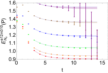
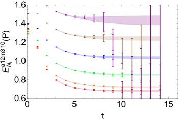
Figure 1: Nucleon effective-mass plots for $M_{\pi}\approx 690$ MeV (left) and $M_{\pi}\approx 310$ MeV (right) at $z=0$, $P_{z}=[0,5]\times\frac{2\pi}{L}$ on the a12m310 ensemble. The bands are reconstructed from the two-state fitted parameters of two-point correlators. The momentum $P_{z}=5\frac{2\pi}{L}$ is the largest momentum we used, and it is the noisiest data set.

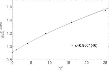
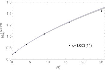
Figure 2: Dispersion relations of the nucleon energy from the two-state fits for $M_{\pi}\approx 690$ MeV (left) and $M_{\pi}\approx 310$ MeV (right)

We use the unpolarized gluon operator defined in Ref. Balitsky et al. (2020),

$${\cal O}_{g}(z) \equiv\sum_{i\neq z,t}{\cal O}(F^{ti},F^{ti};z)-\sum_{i,j\neq z,t}{\cal O}(F^{ij},F^{ij};z),$$ (5)

where the operator ${\cal O}(F^{\mu\nu},F^{\alpha\beta};z)=F^{\mu}{}_{\nu}(z)U(z,0)F^{\alpha}{}_{\beta}(0)$, $z$ is the Wilson link length and the field tensor $F_{\mu\nu}$ is defined as,

$$F_{\mu\nu}=\frac{i}{8a^{2}g_{0}}(\mathcal{P}_{[\mu,\nu]}+\mathcal{P}_{[\nu,-\mu]}+\mathcal{P}_{[-\mu,-\nu]}+\mathcal{P}_{[-\nu,\mu]}),$$ (6)

where the $a$ is the lattice spacing, $g_{0}$ is the strong coupling constant, the plaquette $\mathcal{P_{\mu,\nu}}=U_{\mu}(x)U_{\nu}(x+a\hat{\mu})U^{{\dagger}}_{\mu}(x+a\hat{\nu})U^{{\dagger}}_{\nu}(x)$ and $\mathcal{P_{[\mu,\nu]}}=\mathcal{P}_{\mu,\nu}-\mathcal{P}_{\nu,\mu}$. The operator $O_{g}$ is chosen because its corresponding matching kernel appears in Ref. Balitsky et al. (2020). An alternative operator, $\sum_{i\neq z,t}{\cal O}(F^{ti},F^{zi};z)$, vanishes at $P_{z}=0$ for kinematic reasons, which would cause additional difficulty in obtaining the distributions from this operator. We find the bare matrix elements to be consistent with up to 5 HYP-smearing steps, and the signal-to-noise ratios do not improve much with more steps. For the gluon operator used in this paper, we use 4 HYP smearing steps to reduce the statistical uncertainties, as studied in Ref. Fan et al. (2018).

We obtain the three-point gluon correlator by combining the gluon loop with nucleon two-point correlators,

$$C_{N}^{\text{3pt}}(z,P_{z};t_{\text{sep}},t)$$

$$=\langle 0|\Gamma\int d^{3}y\,e^{-iyP_{z}}\chi(\vec{y},t_{\text{sep}}){\cal O}_{g}(z,t)\chi(\vec{0},0)|0\rangle,$$ (7)

where $t$ is the gluon-operator insertion time, $t_{\text{sep}}$ is the source-sink time separation, and ${\cal O}_{g}(z,t)$ is the gluon operator. The matrix elements of gluon operators can be obtained by fitting the three-point function to its energy-eigenstate expansion,

$$C_{N}^{\text{3pt}}(z,P_{z},t,t_{\text{sep}})$$ (8)

$$=|A_{N,0}|^{2}\langle 0|O_{g}|0\rangle e^{-E_{N,0}t_{\text{sep}}}$$

$$+|A_{N,0}||A_{N,1}|\langle 0|O_{g}|1\rangle e^{-E_{N,1}(t_{\text{sep}}-t)}e^{-E_{N,0}t}$$

$$+|A_{N,0}||A_{N,1}|\langle 1|O_{g}|0\rangle e^{-E_{N,0}(t_{\text{sep}}-t)}e^{-E_{N,1}t}$$

$$+|A_{N,1}|^{2}\langle 1|O_{g}|1\rangle e^{-E_{N,1}t_{\text{sep}}}+...,$$

where the amplitudes and energies, $A_{N,0}$, $A_{N,1}$, $E_{N,0}$ and $E_{N,1}$ are obtained from the two-state fit of the 2-point correlator. $\langle 0|O_{g}|0\rangle$, $\langle 0|O_{g}|1\rangle$ ($\langle 1|O_{g}|0\rangle$), and $\langle 1|O_{g}|1\rangle$ are the ground state matrix element, ground-excited state matrix element, and excited state matrix element respectively. The ground state matrix element $\langle 0|O_{g}|0\rangle$ is obtained from either a “two-sim” fit, a two-state simultaneous fit on multiple separation times with the $\langle 0|O_{g}|0\rangle,\langle 0|O_{g}|1\rangle,\langle 1|O_{g}|0\rangle$ terms, or a “two-simRR” fit, which also includes the $\langle 1|O_{g}|1\rangle$ term.

Figure 3 shows example correlator plots from the ratio

$$R_{N}(P_{z},t,t_{\text{sep}})=\frac{C_{N}^{\text{3pt}}(P_{z},t,t_{\text{sep}})}{C_{N}^{\text{2pt}}(P_{z},t_{\text{sep}})}.$$ (9)

as a function of the $t-t_{\text{sep}}/2$ for multiple source-sink separations for at $P_{z}=2\times 2\pi/L$ and $t_{\text{sep}}=\{6,7,8,9\}\times a$. The reconstructed ratio plot, using the fitted parameters obtained from Eqs. (8) and (4) are plotted for each $t_{\text{sep}}$, and the gray band indicates the reconstructed ground-state matrix elements $\langle 0|{\cal O}_{g}|0\rangle$. The left-two plots in Fig. 3 show the two-simRR fits and two-sim fits using the $t_{\text{sep}}=\{6,7,8,9\}a$, while the remaining two plots show individual two-state fits to the smallest and largest source-sink separations ($t_{\text{sep}}=\{6,9\}a$). The plots of pion mass $M_{\pi}\approx 690$ MeV and $M_{\pi}\approx 310$ MeV are shown in the first row and second row respectively. The reconstructed ground state matrix elements (gray bands) for $O_{g}$ are consistent for the fits with individual $t_{\text{sep}}=\{6,9\}$, the two-sim fit results and the two-simRR fit within one sigma error. Therefore, the two-sim fits describe data from $t_{\text{sep}}=\{6,7,8,9\}$ well for operator $O_{g}$. Thus, we use the two-sim fits to extract the ground-state matrix element $\langle 0|O_{g}|0\rangle$ of different $z$, $P_{z}$ for the rest of this paper.

Our extracted bare ground-state matrix elements are stable across various fit ranges. Figure 4 shows example results from $M_{\pi}\approx 690$ MeV and $M_{\pi}\approx 310$ MeV nucleons with nucleon momentum $P_{z}\in[1,5]\times 2\pi/L$ as the fit ranges for two- and three-point varies. In this case, the two-point correlator fit ranges are $[t_{\text{min}},13]$ and the three-point correlators fit ranges are $[t_{\text{skip}},t_{\text{sep}}-t_{\text{skip}}]$. All the matrix elements from different fit ranges are consistent with each other in one-sigma error. The fit range choice $t_{\text{skip}}^{\text{3pt}}=1$, $t_{\text{min}}^{\text{2pt}}=2$ are not used, because the $\chi^{2}/\text{dof}$ of the 2-point correlator fits with $t_{\text{min}}^{\text{2pt}}=2$ are much larger than the $t_{\text{min}}^{\text{2pt}}=3$ cases. For the rest of this paper, we use the fitted matrix elements obtained from the fit-range choice $t_{\text{skip}}^{\text{3pt}}=1$, $t_{\text{min}}^{\text{2pt}}=3$. The extracted bare matrix elements are fitted for $P_{z}\in[0,5]\times 2\pi/L$ and $z\in[0,5]\times a$ to obtain the Ioffe-time distributions in pseudo-PDF calculation.

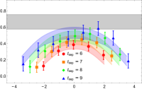
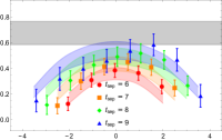
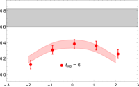
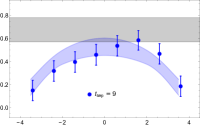
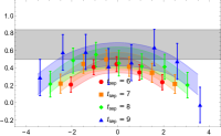
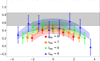
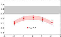
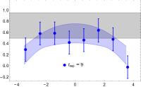
Figure 3: The three-point ratio plots for $M_{\pi}\approx 690$ MeV (top row) and $M_{\pi}\approx 310$ MeV (bottom row)nucleons $z=1$ as functions of $t-t_{\text{sep}}/2$, as defined in Eq. 9. The results for nucleon momentum $P_{z}=2\times 2\pi/L$ are shown. The gray bands in each panel indicate the extracted ground-state matrix elements of the operator $O_{g}$. In each column, the plots show the fitted ratio and the extracted ground-state matrix elements from two-simRR and two-sim fits with all 4 source-sink separations, and the two-state fits using only the smallest and largest $t_{\text{sep}}$ from left to right, respectively. The second column, which are the two-sim extracted ground-state matrix elements, are used in the subsequent analysis. The ground-state matrix elements extracted are stable and consistent among different fitting methods and three-point data input used.

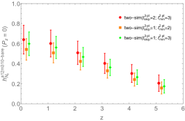
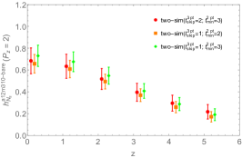
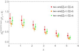
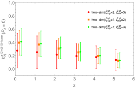
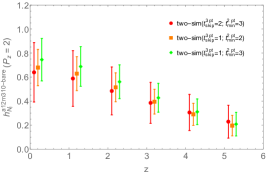
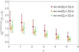
Figure 4: The fitted bare ground-state matrix elements without normalization by kinematic factors as functions of $z$ obtained from the two-sim fit using different two- and three-point fit ranges for nucleon momentum $P_{z}\in\{0,2,4\}\times 2\pi/L$ from left to right, respectively, for $M_{\pi}\approx 690$ MeV (first row) and $M_{\pi}\approx 310$ MeV (second row) nucleons. The green points, which represent the fit-range choice $t_{\text{skip}}^{\text{3pt}}=1$, $t_{\text{min}}^{\text{2pt}}=3$ are used in the following analysis, because the errors of the matrix elements of this fit range are relatively smaller than the error of the red points. The orange points, which represent the fit-range choice $t_{\text{skip}}^{\text{3pt}}=1$, $t_{\text{min}}^{\text{2pt}}=2$, are not used because the $\chi^{2}/\text{dof}$ of the 2-point correlator fits with $t_{\text{min}}^{\text{2pt}}=2$ are much larger than $t_{\text{min}}^{\text{2pt}}=3$ cases.

III Results and Discussions

In the previous section, we obtained the gluon ground-state bare matrix element $\langle 0|{\cal O}_{g}(z)|0\rangle$ at different $z$ and $P_{z}$. The Ioffe-time distribution (ITD) $\mathcal{M}(\nu,z^{2})$ is

$$\mathcal{M}(\nu,z^{2})=\langle 0|{\cal O}_{g}(z)|0\rangle,$$ (10)

where Ioffe time $\nu=zP_{z}$. We construct the reduced ITD, where we take the ratio of the ITD with its value at $\nu=0$, to eliminate ultraviolet divergences. We then further normalize the ratio by the reduced ITD at $z^{2}=0$ to cancel out the kinematic factors and improve the signal-to-noise ratios. The resulting double ratio Orginos et al. (2017) is

$$\mathscr{M}(\nu,z^{2})=\frac{\mathcal{M}(\nu,z^{2})/\mathcal{M}(\nu,0)}{\mathcal{M}(0,z^{2})/\mathcal{M}(0,0)}.$$ (11)

Dividing up the matrix elements by their corresponding boost momentum at $z=0$ also has the advantages of reducing the statistical and lattice systematic errors, and has been done since the first Bjorken-$x$–dependent PDF calculation Lin (2014b) in 2013. One of the reasons we use operator $O_{g}$ is that unlike other nonperturbatively renormalizable operators, it gives nonzero results at $P_{z}=0$. This makes it a better choice to form the reduced pseudo-ITD by taking a double ratio, as discussed in Ref. Balitsky et al. (2020). The reduced-ITD double ratios used here have no additional explicit normalization Orginos et al. (2017), and one can apply the pseudo-PDF matching condition Balitsky et al. (2020) to obtain the unpolarized gluon PDF,

$$\mathscr{M}(\nu,z^{2})=\int_{0}^{1}dx\frac{xg(x,\mu^{2})}{\langle x_{g}\rangle_{\mu^{2}}}R(x\nu,z^{2}\mu^{2}),$$ (12)

where $\mu$ is the renormalization scale in $\overline{\text{MS}}$ scheme and $\langle x_{g}\rangle_{\mu^{2}}=\int_{0}^{1}dx\ xf_{g}(x,\mu)$ is the gluon momentum fraction of the nucleon. The matching kernel, $R(y=x\nu,z^{2}\mu^{2})$, is composed of two terms to deal with the effects of evolution and scheme conversion Radyushkin (2017b),

$$R(y,z^{2}\mu^{2})=R_{1}(y,z^{2}\mu^{2})+R_{2}(y),$$ (13)

$$R_{1}(y,z^{2}\mu^{2})=-\frac{\alpha_{s}(\mu)}{2\pi}N_{c}\ln\left(z^{2}\mu^{2}\frac{e^{2\gamma_{E}+1}}{4}\right)R_{B}(y),$$ (14)

$$R_{2}(y)=\cos y-\frac{\alpha_{s}(\mu)}{2\pi}N_{c}\left(2R_{B}(y)+R_{L}(y)+R_{C}(y)\right),$$ (15)

where $R_{1}(y,z^{2}\mu^{2})$ is the term related to evolution, $R_{2}(y,z^{2}\mu^{2})$ is the term related to scheme conversion, $\alpha_{s}$ is the strong coupling at scale $\mu$, $N_{c}=3$ is the number of colors, $\gamma_{E}=0.5772$ is Euler-Mascheroni constant, and $R_{B}(y)$, $R_{L}(y)$ and $R_{C}(y)$ are defined in Eqs. 7.21–23 in Ref. Balitsky et al. (2020). The $z$ in $R_{1}(y,z^{2}\mu^{2})$ is chosen to be $e^{-\gamma_{e}-1/2}/\mu$ so that the log term vanishes, suppressing the residuals that contain higher orders of the log term, as discussed in Ref. Radyushkin (2018).

The lightcone PDF at physical pion mass is obtained from the reduced ITDs by the following procedure. First, we extrapolate the reduced ITDs to physical pion mass. Second, we evolve the reduced ITDs. Finally, we assume a functional form for the unpolarized gluon PDF and use the matching kernel to match it to the evolved ITDs to fit with the lattice simulation data. In order to determine the gluon PDF at physical pion mass, we extrapolate our reduced ITD results at $M_{\pi}=690$ and 310 MeV to $M_{\pi}^{\text{phys}}=135$ MeV using the following simple naive ansatz:

$$\mathscr{M}(\nu,z^{2},M_{\pi}) =\mathscr{M}(\nu,z^{2},M_{\pi}^{\text{phys}})$$

$$+K(\nu,z^{2})(M_{\pi}^{2}-(M_{\pi}^{\text{phys}})^{2}),$$ (16)

where $M_{\pi}^{\text{phys}}$ is the physical pion mass. We fit the reduced ITDs for each jackknife sample at each $P_{z}$ and $z$ value. The slope $K$ is about $-0.05\text{ GeV}^{-2}$ in our fit. Then, the jackknife samples of the reduced ITDs at physical pion mass are reconstructed from the fit parameters from each jackknife sample fit. Figure 5 shows the extrapolation results for the reduced ITDs at $P_{z}\in\{1,5\}\times 2\pi/L$.

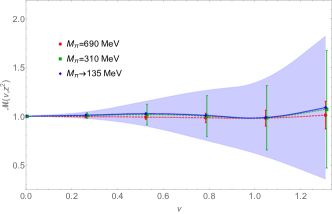
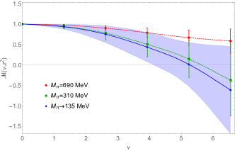
Figure 5: The reduced ITDs $\mathscr{M}(\nu,z^{2})$ as functions of $\nu$ and their extrapolation to the physical pion mass at $P_{z}=1\times 2\pi/L$ (left) and $P_{z}=5\times 2\pi/L$ (right). The blue bands represent the fitted results of the reduced ITDs at the physical pion mass $M_{\pi}=135$ MeV.

The evolved ITD $G$ is obtained by using the evolution term $R_{1}(y,z^{2}\mu^{2})$ in Eq. 14,

$$G(\nu,z^{2},\mu,M_{\pi}) =\mathscr{M}(\nu,z^{2},M_{\pi})$$

$$+\int^{1}_{0}\text{d}uR_{1}(u,z^{2}\mu^{2})\mathscr{M}(u\nu,z^{2},M_{\pi}).$$ (17)

To obtain the evolved ITD, we interpolate the reduced ITD $\mathscr{M}(\nu,z^{2})$ to be a continuous function of $\nu$, using “$z$-expansion” fit Boyd et al. (1995); Bourrely et al. (2009) (also adopted by past pseudo-PDF calculations Joó et al. (2019b))

$$\mathscr{M}(\nu,z^{2},M_{\pi})=\sum_{k=0}^{k_{\text{max}}}\lambda_{k}\tau^{k},$$ (18)

where $\tau=\frac{\sqrt{\nu_{\text{cut}}+\nu}-\sqrt{\nu_{\text{cut}}}}{\sqrt{\nu_{\text{cut}}+\nu}+\sqrt{\nu_{\text{cut}}}}$. Then, we use the fitted $\mathscr{M}(\nu,z^{2})$ in the integral in Eq. 17. The $z$-dependence in the $\mathscr{M}(u\nu,z^{2})$ term in the evolution function comes from the one-loop matching term, which is a higher-order correction compared to the tree-level term; thus, the $z$-dependence can be neglected in $\mathscr{M}(\nu,z^{2})$. We choose the dimensionless cutoff $\nu_{\text{cut}}=1$ as used in the past pseudo PDF calculation Joó et al. (2019b). We also vary $\nu_{\text{cut}}$ between [0.5,2] and the results are consistent with each other. We fix the $\lambda_{0}=1$ because of the normalization we have for the reduced ITD $\mathscr{M}(\nu,z^{2})$ in Eq. 11. The maximum term $k_{\text{max}}=3$ is used, because we can fit all the data points $P_{z}\in[1,5]$ and $z\in[1,5]\times a$ with small $\chi^{2}$ using a 4-term $z$-expansion.

As shown in Fig. 6, the reduced ITDs of different $z^{2}$ from our lattice calculation show very little $z$ dependence, because the $z$ dependence cancels out when dividing out the ITD at $P=0$ in the ratio defining the reduced ITD. Our fitted bands from the $z$-expansion fit match the reduced ITDs at different pion masses within the error bands. In Fig. 6, we can see that the fitted bands are mostly controlled by the small-$z$ reduced ITDs, because the error grows significantly with increasing $z$. The reduced ITDs at physical pion mass are extrapolated from the pion masses at $M_{\pi}=690$ and 310 MeV and are closer to the smaller pion mass at $M_{\pi}=310$ MeV. As $\nu$ grows, the reduced ITDs decrease from $\mathcal{M}(0,z^{2})=1$. The decrease becomes faster when we go to smaller pion masses, but this trend is slight because the pion-mass dependence is weak in our case, as seen in Fig. 6, where the data and the fitted bands from 3 different pion masses are consistent within one sigma error.

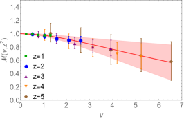
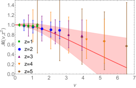
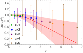
Figure 6: The reduced ITDs $\mathscr{M}(\nu,z^{2})$ as functions of $\nu$ at pion masses $M_{\pi}=690$, 310 and extrapolated 135 MeV from left to right, respectively. The points of different colors represent the reduced ITDs $\mathscr{M}(\nu,z^{2})$ of different $z^{2}$ and the red band represents the $z$-expansion fit band.

The evolved ITDs at $M_{\pi}=690$, 310 and extrapolated 135 MeV are obtained from Eq. 17. In the evolution, we choose $\mu=2$ GeV and $\alpha_{s}(2\text{ GeV})=0.304$. The $z$ dependence of the evolved ITDs should be compensated by the $\ln{z^{2}}$ term in the evolution formula, which is confirmed in our evolution results. The evolved ITDs from different $z\in[1,5]\times a$ are shown in Fig. 7 as points with different colors and are consistent with each other within one sigma error. Similar to the reduced ITDs, the evolved ITDs show small pion-mass dependence, because the data points from 3 different pion mass are consistent within one sigma error. According to the evolution function in Eq. 14, we can obtain the evolved ITD $G$ by adding the reduced ITD $\mathscr{M}$ and an integral term related to $\mathscr{M}$. Due to the cancellation between the two terms, this can reduce the error in the evolved ITDs. This phenomenon is also seen in other pseudo-PDF calculations Joó et al. (2019a); Bhat et al. (2020).

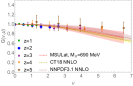
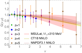
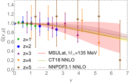
Figure 7: The evolved ITDs $G$ as functions of $\nu$ at pion masses $M_{\pi}\approx 690$, 310 and extrapolated 135 MeV from left to right, respectively. The points of different colors represent the evolved ITDs $G(\nu,z^{2})$ of different $z$ values. The red band represents the fitted band of evolved ITD matched from the functional form PDF using the matching formula Eq. 20. The yellow and pink bands represent the evolved ITD matched from the CT18 NNLO and NNPDF3.1 NNLO unpolarized gluon PDF, respectively. The evolution and matching are both performed at $\mu=2$ GeV in the $\overline{\text{MS}}$ scheme.

We assume a functional form for the lightcone PDF to fit the evolved ITD,

$$f_{g}(x,\mu)=\frac{xg(x,\mu)}{\langle x_{g}\rangle_{\mu^{2}}}=\frac{x^{A}(1-x)^{C}}{B(A+1,C+1)},$$ (19)

for $x\in[0,1]$ and zero elsewhere. The beta function $B(A+1,C+1)=\int_{0}^{1}dx\,x^{A}(1-x)^{C}$ is used to normalize the area to unity. The $xg(x,\mu)$ can be reconstructed by multiplying the gluon momentum fraction $\langle x_{g}\rangle_{\mu^{2}}=0.411(8)$ Constantinou et al. (2020) back to the fit form. Then, we apply the matching formula to obtain the evolved ITD,

$${G}(\nu,\mu)=\int_{0}^{1}dx\,f_{g}(x,\mu)R_{2}(x\nu).$$ (20)

We then fit the evolved ITD ${G}$ from the functional form PDF to the evolved ITD $G$ from the lattice calculation. The fits are performed by minimizing the $\chi^{2}$ function,

$$\chi^{2}=\sum_{\nu,z}\frac{({G}(\nu,\mu)-{G}(\nu,z^{2},\mu,M_{\pi}))^{2}}{\sigma^{2}_{{G}}(\nu,z^{2},\mu,M_{\pi})}.$$ (21)

The fit is performed on the evolved ITDs for $M_{\pi}=690$, 310 and extrapolated 135 MeV separately. The fitted evolved ITD represented by the red band shows a decreasing trend as $\nu$ increases. The fit results for three pion masses are consistent with each other, as well as the evolved ITD from CT18 NNLO and NNPDF3.1 NNLO gluon unpolarized PDF, within one sigma error. However, the rate at which it decreases for smaller pion mass is slightly faster. The fit parameters and the goodness of the fit, $\chi^{2}/\text{dof}$, are summarized in Table 2. From the functional form, it is obvious that parameter $A$ constrains the small-$x$ behaviour and parameter $C$ constrains the large-$x$ behaviour. However, the small-$x$ results obtained from the lattice calculation are not reliable. This is because the Fourier transform of the Ioffe time $\nu$ is related to the region around the inverse of the $x$ and the large-$\nu$ results of evolved ITDs as shown in Fig. 7 have large error, which leads to poor constraint on the small-$x$ behaviour of $xg(x,\mu)$. In contrast, the large-$x$ behaviour of $xg(x,\mu)$ is constrained well because of the small error in the evolved ITDs in the small-$\nu$ region. Therefore, we have a plot that specifically shows the large-$x$ region of $x^{2}g(x,\mu)$ in Fig. 8.

$M_{\pi}$ (MeV)	$A$	$C$	$\chi^{2}/\text{dof}$
690	$-0.622(14)$	$2.5(13)$	$0.35(45)$
310	$-0.611(8)$	$2.3(23)$	$0.19(36)$
135 (extrapolated)	$-0.611(9)$	$2.2(24)$	$0.19(38)$

Table 2: Our gluon PDF fit parameters, $A$ and $C$, from Eq. 19, and goodness of the fit, $\chi^{2}/\text{dof}$, for calculations at two valence pion masses and the extrapolated physical pion mass.

A comparison of our unpolarized gluon PDF with CT18 NNLO and NNPDF3.1 NNLO at $\mu=2$ GeV in the $\overline{\text{MS}}$ scheme is shown in Fig. 8. We compare our $xg(x,\mu)/\langle x_{g}\rangle_{\mu^{2}}$ with the phenomenological curves in the left panel. The middle panel shows the same comparison for $xg(x,\mu)$. Our $xg(x,\mu)$ extrapolated to the physical pion mass $M_{\pi}=135$ MeV is close to the 310-MeV results and there is only mild pion-mass dependence compared with the 690-MeV results. We found that our gluon PDF is consistent with the one from CT18 NNLO and NNPDF3.1 NNLO within one sigma in the $x>0.3$ region. However, in the small-$x$ region ($x<0.3$), there is a strong deviation between our lattice results and the global fits. This is likely due to the fact that the largest $\nu$ used in this calculation is less than 7, and the errors in large-$\nu$ data increase quickly as $\nu$ increases. To better see the large-$x$ behavior, we multiply an additional $x$ factor into the fitted $xg(x,\mu)$ and zoom into the range $x\in[0.5,1]$ in the rightmost plot of Fig. 8. Our large-$x$ results are consistent with global fits over $x\in[0.5,1]$ though with larger errorbars, except for $x\in[0.9,1]$ where our error is smaller than NNPDF, likely due to using fewer parameters in the fit. With improved calculation and systematics in the future, lattice gluon PDFs can show promising results.

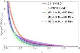
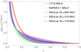
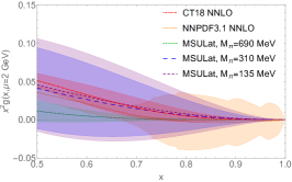
Figure 8: The unpolarized gluon PDF, $xg(x,\mu)/\langle x_{g}\rangle_{\mu^{2}}$ (left), $xg(x,\mu)$ (middle), $x^{2}g(x,\mu)$ in the large-$x$ region as a function of $x$ (right), obtained from the fit to the lattice data at pion masses $M_{\pi}=135$ (extrapolated), 310 and 690 MeV compared with the CT18 NNLO (red band with dot-dashed line) and NNPDF3.1 NNLO (orange band with solid line) gluon PDFs. Our $x>0.3$ PDF results are consistent with the CT18 NNLO and NNPDF3.1 NNLO unpolarized gluon PDFs at $\mu=2$ GeV in the $\overline{\text{MS}}$ scheme.

To demonstrate the influence of the large-$\nu$ data on the fit results, we perform fits to the evolved ITDs with $\nu_{\text{max}}$ of 3 and 4, comparing with the original fits with $\nu_{\text{max}}=6.54$. The fits with the $\nu_{\text{max}}$ cutoff are implemented on the lattice-calculated evolved ITDs and the evolved ITDs created by matching the CT18 NNLO gluon PDF. We show the evolved ITDs from the $M_{\pi}=310$ MeV lattice data and the fitted bands on the left-hand side of Fig. 9. The errors of the fit bands become smaller as larger-$\nu_{\text{max}}$ data are included even though the errors in the input points increases. As a result, we can see in the middle of Fig. 9 that the lattice gluon PDF errors shrink when the large-$\nu$ data help to constrain the fit.

Since our ability to accurately determine the PDFs in the small-$x$ region is limited by the $\nu_{\text{max}}$ calculated on the lattice, we study the effect of the $\nu$ cutoff on our obtained $x$-dependent gluon PDF. To do so, we took the CT18 NNLO gluon PDF to construct a set of evolved ITDs using the same cutoffs $\nu_{\text{max}}=\{3,4,6.54\}$ used on the 310-MeV PDF. The right-hand side of Fig. 9 shows that when $\nu_{\text{max}}$ increases, the region the reconstructed PDF can recover extends to smaller $x$. Based on this observation, we estimate that with $\nu_{\text{max}}=6.54$, the smallest $x$ at which our lattice PDF can be trusted is around 0.25. We use the difference between the original CT18 input and the one reconstructed with a $\nu$ cutoff to estimate the systematic due to this cutoff effect on the higher moments.

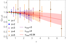
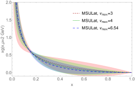
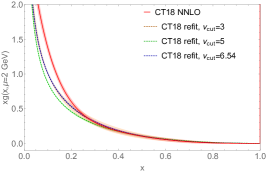
Figure 9: Left: The evolved ITDs $G$ as functions of $\nu$ at $M_{\pi}\approx 310$ MeV with fits performed using different $\nu_{\text{max}}$ cutoff in the evolved ITDs. As we can see from the tightening of the fit band, the evolved ITDs at larger $\nu$ are still useful in constraining the fit despite their larger errors. Middle: The unpolarized gluon PDF obtained from the fits to the evolved ITDs at 310-MeV pion mass with different $\nu_{\text{max}}$. The evolution and matching are both performed at $\mu=2$ GeV in the $\overline{\text{MS}}$ scheme. The larger the $\nu$ input, the more precise the PDF obtained. Right: The 2-GeV $\overline{\text{MS}}$ renormalized unpolarized gluon PDF obtained from a fit to the evolved ITDs generated from the CT18 NNLO PDF with $\nu_{\text{max}}\in\{3,5,6.54\}$, compared with the original CT18 NNLO unpolarized gluon PDFs. As $\nu$ increases, we can see the gluon PDF is better reproduced toward small $x$. Using this exercise, we can see that our lattice PDF is only reliable in the $x>0.25$ region. By taking the moments obtained from CT18 with a cutoff of $\nu_{\text{max}}=6.54$ compared to those from the original PDF, we can estimate the higher-moment systematics in our lattice calculation.

We summarize our predictions for the second and third moments $\langle x_{g}^{2}\rangle_{\mu^{2}}$ and $\langle x_{g}^{3}\rangle_{\mu^{2}}$ at $\mu=2$ GeV with their statistical and systematic errors in Table 3, together with the ones from CT18 NNLO and NNPDF3.1 NNLO results. The first error on our number corresponds to the statistical errors from the calculation, while the second error comes from combining in quadrature the systematic errors from four different sources: 1) The normalization of the global-PDF determination of the moment used in our calculation; 2) The finite-$\nu$ cutoff in the evolved ITDs, as discussed above. 3) The choice of strong coupling constant. To estimate this error, we vary $\alpha_{s}$ by 10%. Like previous pseudo-PDF studies Joó et al. (2019b), we find that the changes are no more than 5%; 4) The mixing with the quark singlet sector. We implement the gluon pseudo-PDF full matching kernel including the quark mixing term on CT18 NNLO unpolarized gluon PDF. The contribution of quark is about $4\%$, which is smaller than systematic errors from other sources. A more precise study of the effects of quark mixing on the unpolarized gluon PDF can be done when we have better control of statistical errors and other systematic errors. Overall, our moments are in agreement with the global-fit results. Future work including lighter pion masses and finer lattice-spacing ensembles will further help us reduce the systematics in the calculation.

moment	MSULat (690 MeV)	MSULat (310 MeV)	MSULat (extrapolated 135 MeV)	CT18	NNPDF3.1
$\langle x_{g}^{2}\rangle_{\mu^{2}}$	0.040(15)(3)	0.043(26)(4)	0.045(30)(4)	0.0552(76)	0.048(13)
$\langle x_{g}^{3}\rangle_{\mu^{2}}$	0.011(6)(2)	0.013(14)(3)	0.014(17)(3)	0.0154(37)	0.011(9)

Table 3: Predictions for the higher gluon moments from this work and the corresponding ones obtained from CT18 NNLO and NNPDF3.1 NNLO global fits. The first error in our number corresponds to the statistical errors from the calculation and the second errors are the systematic errors.

IV Summary and Outlook

In this paper, we present the first lattice calculation of the gluon parton distribution function using the pseudo-PDF method. The current calculation is only done on one ensemble with lattice spacing of 0.12 fm and two valence-quark masses, corresponding to pion masses around 310 and 690 MeV. In contrast to the prior lattice gluon calculation Fan et al. (2018), we now use an improved gluon operator that is proved to be multiplicatively renormalizable. The gluon nucleon matrix elements were obtained using two-state fits. The use of the improved sources in the nucleon two-point correlators allowed us to reach higher nucleon boost momentum. As a result, we were able to attempt to extract the gluon PDF as a function of Bjorken-$x$ for the first time. There are systematics yet to be studied in this work. Future work is planned to study additional ensembles at different lattice spacings so that we can include the lattice-discretization systematics. Lighter quark masses should be used to control the chiral extrapolation to obtain more reliable results at physical pion mass.

References

- Dulat et al. (2016) S. Dulat, T.-J. Hou, J. Gao, M. Guzzi, J. Huston, P. Nadolsky, J. Pumplin, C. Schmidt, D. Stump, and C. P. Yuan, Phys. Rev. D93, 033006 (2016), arXiv:1506.07443 [hep-ph] .
- Harland-Lang et al. (2015) L. A. Harland-Lang, A. D. Martin, P. Motylinski, and R. S. Thorne, Eur. Phys. J. C75, 204 (2015), arXiv:1412.3989 [hep-ph] .
- Ball et al. (2017) R. D. Ball et al. (NNPDF), Eur. Phys. J. C77, 663 (2017), arXiv:1706.00428 [hep-ph] .
- Alekhin et al. (2017) S. Alekhin, J. Blümlein, S. Moch, and R. Placakyte, Phys. Rev. D 96, 014011 (2017), arXiv:1701.05838 [hep-ph] .
- Accardi et al. (2016a) A. Accardi, L. T. Brady, W. Melnitchouk, J. F. Owens, and N. Sato, Phys. Rev. D93, 114017 (2016a), arXiv:1602.03154 [hep-ph] .
- Harland-Lang et al. (2019) L. Harland-Lang, A. Martin, R. Nathvani, and R. Thorne, Eur. Phys. J. C 79, 811 (2019), arXiv:1907.02750 [hep-ph] .
- Bertone et al. (2018) V. Bertone, S. Carrazza, N. P. Hartland, and J. Rojo (NNPDF), SciPost Phys. 5, 008 (2018), arXiv:1712.07053 [hep-ph] .
- Manohar et al. (2017) A. V. Manohar, P. Nason, G. P. Salam, and G. Zanderighi, JHEP 12, 046 (2017), arXiv:1708.01256 [hep-ph] .
- Czakon et al. (2013) M. Czakon, M. L. Mangano, A. Mitov, and J. Rojo, JHEP 07, 167 (2013), arXiv:1303.7215 [hep-ph] .
- Gauld et al. (2015) R. Gauld, J. Rojo, L. Rottoli, and J. Talbert, JHEP 11, 009 (2015), arXiv:1506.08025 [hep-ph] .
- Accardi et al. (2016b) A. Accardi et al., Eur. Phys. J. A 52, 268 (2016b), arXiv:1212.1701 [nucl-ex] .
- Yang et al. (2018a) Y.-B. Yang, M. Gong, J. Liang, H.-W. Lin, K.-F. Liu, D. Pefkou, and P. Shanahan, Phys. Rev. D 98, 074506 (2018a), arXiv:1805.00531 [hep-lat] .
- Yang et al. (2018b) Y.-B. Yang, J. Liang, Y.-J. Bi, Y. Chen, T. Draper, K.-F. Liu, and Z. Liu, Phys. Rev. Lett. 121, 212001 (2018b), arXiv:1808.08677 [hep-lat] .
- Alexandrou et al. (2020) C. Alexandrou, S. Bacchio, M. Constantinou, J. Finkenrath, K. Hadjiyiannakou, K. Jansen, G. Koutsou, H. Panagopoulos, and G. Spanoudes, Phys. Rev. D 101, 094513 (2020), arXiv:2003.08486 [hep-lat] .
- Alexandrou et al. (2017a) C. Alexandrou, M. Constantinou, K. Hadjiyiannakou, K. Jansen, C. Kallidonis, G. Koutsou, A. Vaquero Avilés-Casco, and C. Wiese, Phys. Rev. Lett. 119, 142002 (2017a), arXiv:1706.02973 [hep-lat] .
- Sufian et al. (2017) R. S. Sufian, Y.-B. Yang, A. Alexandru, T. Draper, J. Liang, and K.-F. Liu, Phys. Rev. Lett. 118, 042001 (2017), arXiv:1606.07075 [hep-ph] .
- Shanahan and Detmold (2019) P. Shanahan and W. Detmold, Phys. Rev. D 99, 014511 (2019), arXiv:1810.04626 [hep-lat] .
- Ji (2013) X. Ji, Phys. Rev. Lett. 110, 262002 (2013), arXiv:1305.1539 [hep-ph] .
- Ji (2014) X. Ji, Sci. China Phys. Mech. Astron. 57, 1407 (2014), arXiv:1404.6680 [hep-ph] .
- Ji et al. (2017) X. Ji, J.-H. Zhang, and Y. Zhao, Nucl. Phys. B924, 366 (2017), arXiv:1706.07416 [hep-ph] .
- Ma and Qiu (2018) Y.-Q. Ma and J.-W. Qiu, Phys. Rev. Lett. 120, 022003 (2018), arXiv:1709.03018 [hep-ph] .
- Liu et al. (2019) Y.-S. Liu, W. Wang, J. Xu, Q.-A. Zhang, J.-H. Zhang, S. Zhao, and Y. Zhao, (2019), arXiv:1902.00307 [hep-ph] .
- Bali et al. (2018a) G. S. Bali et al., Proceedings, 35th International Symposium on Lattice Field Theory (Lattice 2017): Granada, Spain, June 18-24, 2017, Eur. Phys. J. C78, 217 (2018a), arXiv:1709.04325 [hep-lat] .
- Bali et al. (2018b) G. S. Bali, V. M. Braun, B. Gläßle, M. Göckeler, M. Gruber, F. Hutzler, P. Korcyl, A. Schäfer, P. Wein, and J.-H. Zhang, Phys. Rev. D 98, 094507 (2018b), arXiv:1807.06671 [hep-lat] .
- Sufian et al. (2019) R. S. Sufian, J. Karpie, C. Egerer, K. Orginos, J.-W. Qiu, and D. G. Richards, Phys. Rev. D 99, 074507 (2019), arXiv:1901.03921 [hep-lat] .
- Sufian et al. (2020) R. S. Sufian, C. Egerer, J. Karpie, R. G. Edwards, B. Joó, Y.-Q. Ma, K. Orginos, J.-W. Qiu, and D. G. Richards, (2020), arXiv:2001.04960 [hep-lat] .
- Orginos et al. (2017) K. Orginos, A. Radyushkin, J. Karpie, and S. Zafeiropoulos, Phys. Rev. D96, 094503 (2017), arXiv:1706.05373 [hep-ph] .
- Karpie et al. (2018a) J. Karpie, K. Orginos, A. Radyushkin, and S. Zafeiropoulos, EPJ Web Conf. 175, 06032 (2018a), arXiv:1710.08288 [hep-lat] .
- Karpie et al. (2018b) J. Karpie, K. Orginos, and S. Zafeiropoulos, JHEP 11, 178 (2018b), arXiv:1807.10933 [hep-lat] .
- Karpie et al. (2019) J. Karpie, K. Orginos, A. Rothkopf, and S. Zafeiropoulos, JHEP 04, 057 (2019), arXiv:1901.05408 [hep-lat] .
- Joó et al. (2019a) B. Joó, J. Karpie, K. Orginos, A. Radyushkin, D. Richards, and S. Zafeiropoulos, JHEP 12, 081 (2019a), arXiv:1908.09771 [hep-lat] .
- Joó et al. (2019b) B. Joó, J. Karpie, K. Orginos, A. V. Radyushkin, D. G. Richards, R. S. Sufian, and S. Zafeiropoulos, Phys. Rev. D 100, 114512 (2019b), arXiv:1909.08517 [hep-lat] .
- Radyushkin (2018) A. Radyushkin, Phys. Rev. D98, 014019 (2018), arXiv:1801.02427 [hep-ph] .
- Zhang et al. (2018) J.-H. Zhang, J.-W. Chen, and C. Monahan, Phys. Rev. D97, 074508 (2018), arXiv:1801.03023 [hep-ph] .
- Izubuchi et al. (2018) T. Izubuchi, X. Ji, L. Jin, I. W. Stewart, and Y. Zhao, Phys. Rev. D98, 056004 (2018), arXiv:1801.03917 [hep-ph] .
- Joó et al. (2020) B. Joó, J. Karpie, K. Orginos, A. V. Radyushkin, D. G. Richards, and S. Zafeiropoulos, (2020), arXiv:2004.01687 [hep-lat] .
- Bhat et al. (2020) M. Bhat, K. Cichy, M. Constantinou, and A. Scapellato, (2020), arXiv:2005.02102 [hep-lat] .
- Xiong et al. (2014) X. Xiong, X. Ji, J.-H. Zhang, and Y. Zhao, Phys. Rev. D90, 014051 (2014), arXiv:1310.7471 [hep-ph] .
- Ji and Zhang (2015) X. Ji and J.-H. Zhang, Phys. Rev. D92, 034006 (2015), arXiv:1505.07699 [hep-ph] .
- Ji et al. (2015a) X. Ji, A. Schäfer, X. Xiong, and J.-H. Zhang, Phys. Rev. D 92, 014039 (2015a), arXiv:1506.00248 [hep-ph] .
- Xiong and Zhang (2015) X. Xiong and J.-H. Zhang, Phys. Rev. D92, 054037 (2015), arXiv:1509.08016 [hep-ph] .
- Ji et al. (2015b) X. Ji, P. Sun, X. Xiong, and F. Yuan, Phys. Rev. D91, 074009 (2015b), arXiv:1405.7640 [hep-ph] .
- Lin (2014a) H.-W. Lin, PoS LATTICE2013, 293 (2014a).
- Monahan (2018) C. Monahan, Phys. Rev. D97, 054507 (2018), arXiv:1710.04607 [hep-lat] .
- Ji et al. (2018a) X. Ji, L.-C. Jin, F. Yuan, J.-H. Zhang, and Y. Zhao, (2018a), arXiv:1801.05930 [hep-ph] .
- Stewart and Zhao (2018) I. W. Stewart and Y. Zhao, Phys. Rev. D97, 054512 (2018), arXiv:1709.04933 [hep-ph] .
- Constantinou and Panagopoulos (2017) M. Constantinou and H. Panagopoulos, Phys. Rev. D96, 054506 (2017), arXiv:1705.11193 [hep-lat] .
- Green et al. (2018) J. Green, K. Jansen, and F. Steffens, Phys. Rev. Lett. 121, 022004 (2018), arXiv:1707.07152 [hep-lat] .
- Xiong et al. (2017) X. Xiong, T. Luu, and U.-G. Meißner, (2017), arXiv:1705.00246 [hep-ph] .
- Wang et al. (2018) W. Wang, S. Zhao, and R. Zhu, Eur. Phys. J. C78, 147 (2018), arXiv:1708.02458 [hep-ph] .
- Wang and Zhao (2018) W. Wang and S. Zhao, JHEP 05, 142 (2018), arXiv:1712.09247 [hep-ph] .
- Xu et al. (2018a) J. Xu, Q.-A. Zhang, and S. Zhao, Phys. Rev. D97, 114026 (2018a), arXiv:1804.01042 [hep-ph] .
- Chen et al. (2016) J.-W. Chen, S. D. Cohen, X. Ji, H.-W. Lin, and J.-H. Zhang, Nucl. Phys. B911, 246 (2016), arXiv:1603.06664 [hep-ph] .
- Zhang et al. (2017) J.-H. Zhang, J.-W. Chen, X. Ji, L. Jin, and H.-W. Lin, Phys. Rev. D95, 094514 (2017), arXiv:1702.00008 [hep-lat] .
- Ishikawa et al. (2016) T. Ishikawa, Y.-Q. Ma, J.-W. Qiu, and S. Yoshida, (2016), arXiv:1609.02018 [hep-lat] .
- Chen et al. (2017a) J.-W. Chen, X. Ji, and J.-H. Zhang, Nucl. Phys. B915, 1 (2017a), arXiv:1609.08102 [hep-ph] .
- Ji et al. (2018b) X. Ji, J.-H. Zhang, and Y. Zhao, Phys. Rev. Lett. 120, 112001 (2018b), arXiv:1706.08962 [hep-ph] .
- Ishikawa et al. (2017) T. Ishikawa, Y.-Q. Ma, J.-W. Qiu, and S. Yoshida, Phys. Rev. D96, 094019 (2017), arXiv:1707.03107 [hep-ph] .
- Chen et al. (2018a) J.-W. Chen, T. Ishikawa, L. Jin, H.-W. Lin, Y.-B. Yang, J.-H. Zhang, and Y. Zhao, Phys. Rev. D97, 014505 (2018a), arXiv:1706.01295 [hep-lat] .
- Alexandrou et al. (2017b) C. Alexandrou, K. Cichy, M. Constantinou, K. Hadjiyiannakou, K. Jansen, H. Panagopoulos, and F. Steffens, Nucl. Phys. B923, 394 (2017b), arXiv:1706.00265 [hep-lat] .
- Chen et al. (2017b) J.-W. Chen, T. Ishikawa, L. Jin, H.-W. Lin, Y.-B. Yang, J.-H. Zhang, and Y. Zhao, (2017b), arXiv:1710.01089 [hep-lat] .
- Lin et al. (2018a) H.-W. Lin, J.-W. Chen, T. Ishikawa, and J.-H. Zhang (LP3), Phys. Rev. D98, 054504 (2018a), arXiv:1708.05301 [hep-lat] .
- Ishikawa et al. (2019) T. Ishikawa, L. Jin, H.-W. Lin, A. Schäfer, Y.-B. Yang, J.-H. Zhang, and Y. Zhao, Sci. China Phys. Mech. Astron. 62, 991021 (2019), arXiv:1711.07858 [hep-ph] .
- Li (2016) H.-n. Li, Phys. Rev. D94, 074036 (2016), arXiv:1602.07575 [hep-ph] .
- Monahan and Orginos (2017) C. Monahan and K. Orginos, JHEP 03, 116 (2017), arXiv:1612.01584 [hep-lat] .
- Radyushkin (2017a) A. Radyushkin, Phys. Lett. B767, 314 (2017a), arXiv:1612.05170 [hep-ph] .
- Rossi and Testa (2017) G. C. Rossi and M. Testa, Phys. Rev. D96, 014507 (2017), arXiv:1706.04428 [hep-lat] .
- Carlson and Freid (2017) C. E. Carlson and M. Freid, Phys. Rev. D95, 094504 (2017), arXiv:1702.05775 [hep-ph] .
- Hobbs (2018) T. J. Hobbs, Phys. Rev. D97, 054028 (2018), arXiv:1708.05463 [hep-ph] .
- Xu et al. (2018b) S.-S. Xu, L. Chang, C. D. Roberts, and H.-S. Zong, Phys. Rev. D97, 094014 (2018b), arXiv:1802.09552 [nucl-th] .
- Jia et al. (2018) Y. Jia, S. Liang, X. Xiong, and R. Yu, Phys. Rev. D98, 054011 (2018), arXiv:1804.04644 [hep-th] .
- Spanoudes and Panagopoulos (2018) G. Spanoudes and H. Panagopoulos, Phys. Rev. D98, 014509 (2018), arXiv:1805.01164 [hep-lat] .
- Rossi and Testa (2018) G. Rossi and M. Testa, Phys. Rev. D98, 054028 (2018), arXiv:1806.00808 [hep-lat] .
- Liu et al. (2018a) Y.-S. Liu, J.-W. Chen, L. Jin, H.-W. Lin, Y.-B. Yang, J.-H. Zhang, and Y. Zhao, (2018a), arXiv:1807.06566 [hep-lat] .
- Ji et al. (2019a) X. Ji, Y. Liu, and I. Zahed, Phys. Rev. D99, 054008 (2019a), arXiv:1807.07528 [hep-ph] .
- Bhattacharya et al. (2019) S. Bhattacharya, C. Cocuzza, and A. Metz, Phys. Lett. B788, 453 (2019), arXiv:1808.01437 [hep-ph] .
- Radyushkin (2019) A. V. Radyushkin, Phys. Lett. B788, 380 (2019), arXiv:1807.07509 [hep-ph] .
- Zhang et al. (2019a) J.-H. Zhang, X. Ji, A. Schäfer, W. Wang, and S. Zhao, Phys. Rev. Lett. 122, 142001 (2019a), arXiv:1808.10824 [hep-ph] .
- Li et al. (2019) Z.-Y. Li, Y.-Q. Ma, and J.-W. Qiu, Phys. Rev. Lett. 122, 062002 (2019), arXiv:1809.01836 [hep-ph] .
- Braun et al. (2019) V. M. Braun, A. Vladimirov, and J.-H. Zhang, Phys. Rev. D99, 014013 (2019), arXiv:1810.00048 [hep-ph] .
- Ebert et al. (2020a) M. A. Ebert, I. W. Stewart, and Y. Zhao, JHEP 03, 099 (2020a), arXiv:1910.08569 [hep-ph] .
- Ji et al. (2019b) X. Ji, Y. Liu, and Y.-S. Liu, (2019b), arXiv:1911.03840 [hep-ph] .
- Shugert et al. (2020) C. Shugert, X. Gao, T. Izubichi, L. Jin, C. Kallidonis, N. Karthik, S. Mukherjee, P. Petreczky, S. Syritsyn, and Y. Zhao, in 37th International Symposium on Lattice Field Theory (2020) arXiv:2001.11650 [hep-lat] .
- Green et al. (2020) J. R. Green, K. Jansen, and F. Steffens, Phys. Rev. D 101, 074509 (2020), arXiv:2002.09408 [hep-lat] .
- Shanahan et al. (2020) P. Shanahan, M. Wagman, and Y. Zhao, (2020), arXiv:2003.06063 [hep-lat] .
- Lin et al. (2020) H.-W. Lin, J.-W. Chen, Z. Fan, J.-H. Zhang, and R. Zhang, (2020), arXiv:2003.14128 [hep-lat] .
- Ji et al. (2020) X. Ji, Y.-S. Liu, Y. Liu, J.-H. Zhang, and Y. Zhao, (2020), arXiv:2004.03543 [hep-ph] .
- Ebert et al. (2020b) M. A. Ebert, S. T. Schindler, I. W. Stewart, and Y. Zhao, (2020b), arXiv:2004.14831 [hep-ph] .
- Lin (2020) H.-W. Lin, Int. J. Mod. Phys. A 35, 2030006 (2020).
- Lin (2014b) H.-W. Lin, PoS LATTICE2013, 293 (2014b).
- Lin et al. (2015) H.-W. Lin, J.-W. Chen, S. D. Cohen, and X. Ji, Phys. Rev. D91, 054510 (2015), arXiv:1402.1462 [hep-ph] .
- Alexandrou et al. (2015) C. Alexandrou, K. Cichy, V. Drach, E. Garcia-Ramos, K. Hadjiyiannakou, K. Jansen, F. Steffens, and C. Wiese, Phys. Rev. D92, 014502 (2015), arXiv:1504.07455 [hep-lat] .
- Alexandrou et al. (2017c) C. Alexandrou, K. Cichy, M. Constantinou, K. Hadjiyiannakou, K. Jansen, F. Steffens, and C. Wiese, Phys. Rev. D96, 014513 (2017c), arXiv:1610.03689 [hep-lat] .
- Alexandrou et al. (2018a) C. Alexandrou, K. Cichy, M. Constantinou, K. Jansen, A. Scapellato, and F. Steffens, Phys. Rev. Lett. 121, 112001 (2018a), arXiv:1803.02685 [hep-lat] .
- Chen et al. (2018b) J.-W. Chen, L. Jin, H.-W. Lin, Y.-S. Liu, Y.-B. Yang, J.-H. Zhang, and Y. Zhao, (2018b), arXiv:1803.04393 [hep-lat] .
- Zhang et al. (2019b) J.-H. Zhang, J.-W. Chen, L. Jin, H.-W. Lin, A. Schäfer, and Y. Zhao, Phys. Rev. D 100, 034505 (2019b), arXiv:1804.01483 [hep-lat] .
- Alexandrou et al. (2018b) C. Alexandrou, K. Cichy, M. Constantinou, K. Jansen, A. Scapellato, and F. Steffens, Phys. Rev. D98, 091503 (2018b), arXiv:1807.00232 [hep-lat] .
- Lin et al. (2018b) H.-W. Lin, J.-W. Chen, X. Ji, L. Jin, R. Li, Y.-S. Liu, Y.-B. Yang, J.-H. Zhang, and Y. Zhao, Phys. Rev. Lett. 121, 242003 (2018b), arXiv:1807.07431 [hep-lat] .
- Fan et al. (2018) Z.-Y. Fan, Y.-B. Yang, A. Anthony, H.-W. Lin, and K.-F. Liu, Phys. Rev. Lett. 121, 242001 (2018), arXiv:1808.02077 [hep-lat] .
- Liu et al. (2018b) Y.-S. Liu, J.-W. Chen, L. Jin, R. Li, H.-W. Lin, Y.-B. Yang, J.-H. Zhang, and Y. Zhao, (2018b), arXiv:1810.05043 [hep-lat] .
- Wang et al. (2019) W. Wang, J.-H. Zhang, S. Zhao, and R. Zhu, (2019), arXiv:1904.00978 [hep-ph] .
- Lin and Zhang (2019) H.-W. Lin and R. Zhang, Phys. Rev. D100, 074502 (2019).
- Chen et al. (2019) J.-W. Chen, H.-W. Lin, and J.-H. Zhang, (2019), 10.1016/j.nuclphysb.2020.114940, arXiv:1904.12376 [hep-lat] .
- Chai et al. (2020) Y. Chai et al., (2020), arXiv:2002.12044 [hep-lat] .
- Bhattacharya et al. (2020) S. Bhattacharya, K. Cichy, M. Constantinou, A. Metz, A. Scapellato, and F. Steffens, (2020), arXiv:2004.04130 [hep-lat] .
- Zhang et al. (2020a) R. Zhang, H.-W. Lin, and B. Yoon, (2020a), arXiv:2005.01124 [hep-lat] .
- Fan et al. (2020) Z. Fan, X. Gao, R. Li, H.-W. Lin, N. Karthik, S. Mukherjee, P. Petreczky, S. Syritsyn, Y.-B. Yang, and R. Zhang, (2020), arXiv:2005.12015 [hep-lat] .
- Detmold et al. (2019) W. Detmold, R. G. Edwards, J. J. Dudek, M. Engelhardt, H.-W. Lin, S. Meinel, K. Orginos, and P. Shanahan (USQCD), Eur. Phys. J. A 55, 193 (2019), arXiv:1904.09512 [hep-lat] .
- Constantinou et al. (2020) M. Constantinou et al., (2020), arXiv:2006.08636 [hep-ph] .
- Nocera et al. (2014) E. R. Nocera, R. D. Ball, S. Forte, G. Ridolfi, and J. Rojo (NNPDF), Nucl. Phys. B887, 276 (2014), arXiv:1406.5539 [hep-ph] .
- Ethier et al. (2017) J. J. Ethier, N. Sato, and W. Melnitchouk, Phys. Rev. Lett. 119, 132001 (2017), arXiv:1705.05889 [hep-ph] .
- Zhang et al. (2020b) R. Zhang, Z. Fan, R. Li, H.-W. Lin, and B. Yoon, Phys. Rev. D101, 034516 (2020b), arXiv:1909.10990 [hep-lat] .
- Gao et al. (2020) X. Gao, L. Jin, C. Kallidonis, N. Karthik, S. Mukherjee, P. Petreczky, C. Shugert, S. Syritsyn, and Y. Zhao, Phys. Rev. D 102, 094513 (2020), arXiv:2007.06590 [hep-lat] .
- Balitsky et al. (2020) I. Balitsky, W. Morris, and A. Radyushkin, Phys. Lett. B 808, 135621 (2020), arXiv:1910.13963 [hep-ph] .
- Follana et al. (2007) E. Follana, Q. Mason, C. Davies, K. Hornbostel, G. P. Lepage, J. Shigemitsu, H. Trottier, and K. Wong (HPQCD, UKQCD), Phys. Rev. D75, 054502 (2007), arXiv:hep-lat/0610092 [hep-lat] .
- Bazavov et al. (2013) A. Bazavov et al. (MILC), Phys. Rev. D87, 054505 (2013), arXiv:1212.4768 [hep-lat] .
- Hasenfratz and Knechtli (2001) A. Hasenfratz and F. Knechtli, Phys. Rev. D64, 034504 (2001), arXiv:hep-lat/0103029 [hep-lat] .
- Gupta et al. (2017) R. Gupta, Y.-C. Jang, H.-W. Lin, B. Yoon, and T. Bhattacharya, Phys. Rev. D96, 114503 (2017), arXiv:1705.06834 [hep-lat] .
- Bhattacharya et al. (2015a) T. Bhattacharya, V. Cirigliano, S. Cohen, R. Gupta, A. Joseph, H.-W. Lin, and B. Yoon (PNDME), Phys. Rev. D92, 094511 (2015a), arXiv:1506.06411 [hep-lat] .
- Bhattacharya et al. (2015b) T. Bhattacharya, V. Cirigliano, R. Gupta, H.-W. Lin, and B. Yoon, Phys. Rev. Lett. 115, 212002 (2015b), arXiv:1506.04196 [hep-lat] .
- Bhattacharya et al. (2014) T. Bhattacharya, S. D. Cohen, R. Gupta, A. Joseph, H.-W. Lin, and B. Yoon, Phys. Rev. D89, 094502 (2014), arXiv:1306.5435 [hep-lat] .
- Bali et al. (2016) G. S. Bali, B. Lang, B. U. Musch, and A. Schäfer, Phys. Rev. D93, 094515 (2016), arXiv:1602.05525 [hep-lat] .
- Li et al. (2010) A. Li et al. (xQCD), Phys. Rev. D 82, 114501 (2010), arXiv:1005.5424 [hep-lat] .
- Gong et al. (2013) M. Gong et al. (XQCD), Phys. Rev. D 88, 014503 (2013), arXiv:1304.1194 [hep-ph] .
- Radyushkin (2017b) A. V. Radyushkin, Phys. Rev. D96, 034025 (2017b), arXiv:1705.01488 [hep-ph] .
- Boyd et al. (1995) C. Boyd, B. Grinstein, and R. F. Lebed, Phys. Rev. Lett. 74, 4603 (1995), arXiv:hep-ph/9412324 .
- Bourrely et al. (2009) C. Bourrely, I. Caprini, and L. Lellouch, Phys. Rev. D 79, 013008 (2009), [Erratum: Phys.Rev.D 82, 099902 (2010)], arXiv:0807.2722 [hep-ph] .
- Edwards and Joo (2005) R. G. Edwards and B. Joo (SciDAC, LHPC, UKQCD), Nucl. Phys. B Proc. Suppl. 140, 832 (2005), arXiv:hep-lat/0409003 .