Gibbsian T-tessellation model for agricultural landscape characterization

Abstract

A new class of planar tessellations, referred to as T-tessellations, was introduced in ([10]). A completely random T-tessellation model (CRTT) was proposed, and its Gibbsian variants were discussed. A general simulation algorithm of Metropolis-Hastings-Green type was derived for model simulation, involving three local transformations of T-tessellations.

The current paper focuses on statistical inference for Gibbs models of T-tessellations. Statistical methods derived from point pattern analysis are implemented on the example of three agricultural landscapes approximated by T-tessellations. The choice of model statistics is guided by their capacity to highlight the differences between the landscape patterns. Model parameters are estimated by the Monte Carlo Maximum Likelihood method, yielding a baseline for landscapes comparison. In the last part of the paper, a global envelope test based on the empty-space function is proposed for assessing the goodness-of-fit of the model.

Keywords— Gibbsian T-tessellation model, Agricultural landscape, Monte Carlo Maximum Likelihood estimation, Empty-space function

1 Introduction

Tessellations are mathematical representations of space division into cells. This paper focuses on a class of tessellations with internal vertices with three incident edges, two of them subtending a straight angle. Such tessellations are referred to as T-tessellations and may represent various spatial patterns, like those illustrated in Figure (1): cracked soil, agricultural landscapes, burnt wood, patterns on a reptile’s skin. Random T-tessellation models allow for spatial variability of such patterns, generating cells with different sizes and shapes. One of the first random T-tessellation models was proposed by Gilbert ([8]) for representing needle-shaped crystals. A variant of the model providing rectangular cells was studied by Miles and Mackisack ([12]). The stable with respect to iteration (STIT) tessellation model was proposed by Nagel and Weiss ([15]) for modeling random crack networks. Another example of a random T-tessellation was proposed by Arak, Clifford and Surgailis ([2]) in their paper on a random graph model. For the particular choice of the parameters, the model yields T-tessellation patterns.

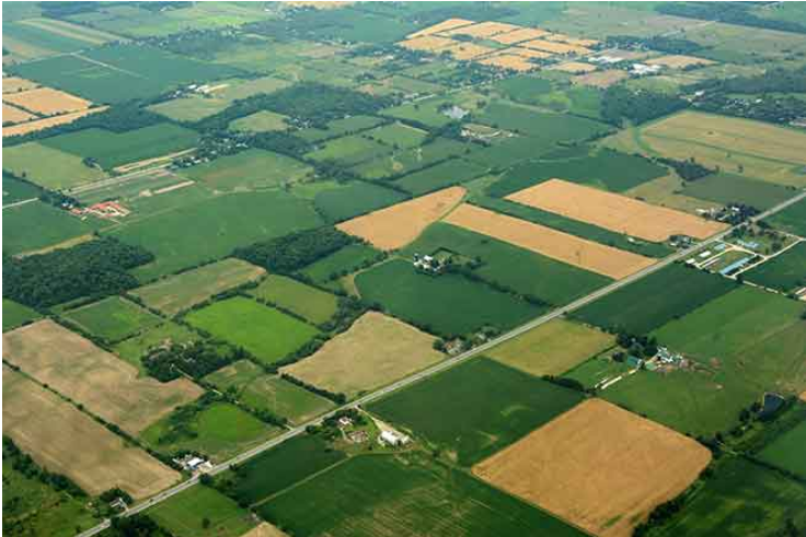
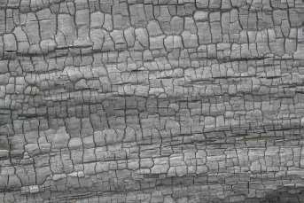
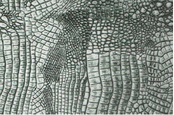
Figure 1: Examples of spatial patterns that may be approximated by a T-tessellation. From upper left panel to lower right one: a cracked soil, an agricultural landscape in Colorado, a texture of burnt wood, a fragment of alligator skin.

More recently, a Completely Random T-Tessellation (CRTT) model was introduced by Kiêu et al. ([10]). The model, based on Poisson line process, was considered as a reference measure on a set of T-tessellations. Gibbs T-tessellations models can be constructed by means of a probability density w.r.t. the CRTT reference measure. The density involves a set of tessellation statistics the model should account for. The tessellations with large (resp. small) values of the targeted statistics are favored by an appropriate tuning of model parameters. The possibility of the model to control various tessellation features makes it attractive for representing a broad scope of the observed T-tessellation patterns. A Metropolis-Hasting-Green algorithm for model simulation was derived in ([10]) and implemented in the C++ library ([1]).

This paper focuses on statistical inference for Gibbsian T-tessellation models. The models parameters were estimated by Monte Carlo Maximum Likelihood (MCML). The estimation method was tested on the example of three agricultural landscapes, approximated by T-tessellations. The models fitted to the landscapes aimed at finding the features responsible for the observed contrasts of landscape structures. The goodness-of-fit of the models was assessed by a global envelope test based on the empty-space function $F$.

The paper is structured as follows. Section (2) describes landscape datasets and presents the algorithm of landscape approximation by a T-tessellation. Section (3) defines the Gibbsian T-tessellation model. The principle of MCML is outlined and the properties of the estimates are investigated by simulations. Section (4) presents the results of model fit to the three datasets and points out the main differences between the landscapes. The goodness-of-fit test is carried out for each dataset. Finally, Section (5) contains the concluding remarks and highlights further perspectives.

2 From landscape data to a T-tessellation

Agricultural landscapes exhibit patterns that can be reasonably approximated by T-tessellations. Indeed, as illustrated in Figure (2), most of the vertices of polygons representing agricultural fields are of the T-type. Although the T-vertices are dominant, actual agricultural landscapes are not T-tessellations and must be modified to match the definition of T-tessellation. In the following, an algorithm for transforming a landscape into a T-tessellation is proposed and tested on three datasets.

2.1 Datasets

Three French agricultural landscapes were selected for the study: the landscape of Selommes (Centre-Val de Loire), an area of intensive cereal crop cultivation; the landscape of Kervidy (Brittany), a region characterized by mixed crop-livestock farming systems; and the landscape of the Basse Valée de la Durance (BVD) in Provence-Alpes-Côte d’Azur region, specialized in apple orchards. Different types of agricultural production characterizing the three regions are in part responsible for the variability of landscape patterns observed in Figure (2). A more detailed presentation of the datasets and the related agroecological research problems can be found in ([17]) for the Selommes landscape, in ([18]) for the Kervidy landscape and in ([19]) for the BVD landscape. The landscapes were restricted to the domains encompassing a comparable number of fields: $230$ for Selommes, $245$ for BVD and $287$ for Kervidy.

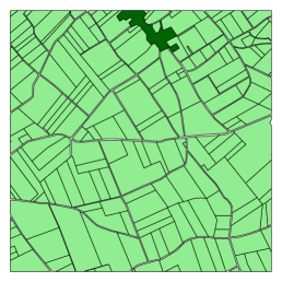
(a)

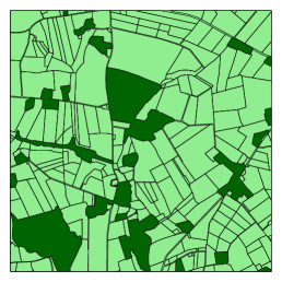
(b)

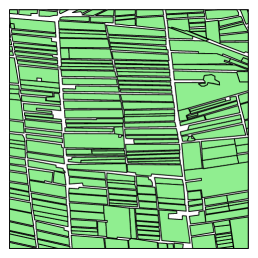
(c)

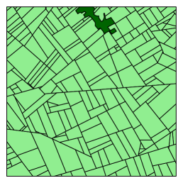
(d)

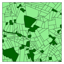
(e)

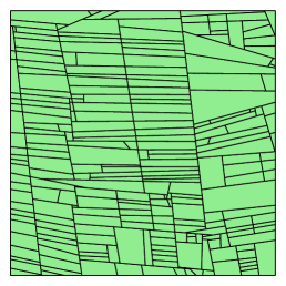
(f)

Figure 2: Upper row: landscapes of Selommes (a); Kervidy (b); and BVD (c). Light green polygons depict agricultural plots, dark green polygons stand for non-agricultural areas (mainly woods and villages). Lower row: landscapes approximated by T-tessellations.

2.2 Landscape approximation algorithm

A polygonal tessellation of a squared domain $W$ is illustrated in Figure (3). The main components of the tessellation are highlighted: the cells, the edges (non-empty intersections of two cells), the vertices (non-empty intersections of three cells) and the segments (maximal unions of the aligned and contiguous edges).

Definition 1.

A polygonal tessellation of a bounded domain $W\subset\mathbb{R}^{2}$ is called a T-tessellation if the following conditions are simultaneously fulfilled:

Condition 1

Each internal vertex of a tessellation has exactly three adjacent edges, two of them subtending the angle of $\pi$.

Condition 2

There is no pair of distinct and aligned segments.

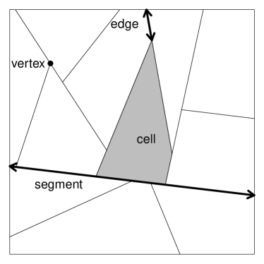
Figure 3: T-tessellation of a squared window.

The purpose of the approximation algorithm is to construct a T-tessellation that closely matches the input set of polygons. The algorithm requires the coordinates of polygons and the coordinates of the tessellated domain, composed from an outer polygon and polygons-holes. The consecutive steps of the algorithm are described below.

Grouping polygons sides (Fig. (4a))

The first step of the algorithm consists of grouping the sides of polygons by hierarchical clustering. Two sides belong to the same group if they are spatially close and if their orientation is similar. The dissimilarity measure that takes these two aspects into account is defined as the sum of two terms: the area of the convex envelope of two sides, denoted by $A(C(.))$, and the smallest Euclidean distance between the sides, denoted by $d_{\min}(.)$:

$$d(c_{i},c_{j})=\frac{A(C(c_{i},c_{j}))}{l(c_{i})l(c_{j})}+\frac{2d_{\min}(c_{i},c_{j})}{{l(c_{i})+l(c_{j})}},$$ (1)

The first term becomes large when the sides $c_{i}$ and $c_{j}$ are far apart and/or perpendicularly oriented; the second one accounts for the distant sides belonging to the same straight line. To make the two components of the criterion independent of the metric, they are normalized by the product of the lengths of the sides and by their average length, respectively. The classification of the sides is based on the single linkage method. In this method, the distance between two groups of sides is defined as the minimal dissimilarity between the pairs of sides from each group. At each step of the algorithm, the two closest groups are merged, starting from the groups containing single sides.

Choice of representative segments (Fig. (4b))

Each group of sides is then replaced by a representative segment: a regression line is fitted to the endpoints of the grouped sides. The projection of each endpoint on the regression line is calculated. A representative segment is the smallest segment on the regression line, including the projections of sides endpoints.

Transformation into T-tessellation (Fig. (4c))

The representative segments are inserted into a tessellation domain, defining a tessellation that is not yet a T-tessellation. It contains the I-vertices with one incident edge, L-vertices with two incident edges, and X-vertices formed by the crossing segments. To remove an I-vertex, the edge can be removed or lengthened until it meets another edge. In order to choose between these two modifications, a variation of total internal length is calculated: the modification that induces the smallest length variation is selected. The same rule also governs the order of removing the I-vertices: at each iteration, the I-vertex whose suppression induces the smallest variation in length is selected. The approach for removing the L-vertices is quite similar: one of two incident edges is lengthened until it meets another edge. The edge that induces the smallest increase in total internal length is selected. The approach for fixing the order of removal of L-vertices is the same as for I-vertices.

In order to remove an X-vertex from a tessellation, one of two segments passing through the vertex is broken into two halves at the vertex location. The end of a segment half lying at the vertex location is moved along the other incident segment by a small distance. The procedure is repeated until there is no X-vertex left in the tessellation.

Figure (2) presents the three landscapes approximated by T-tessellations.

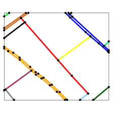
(a)

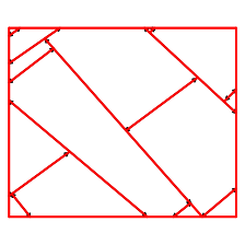
(b)

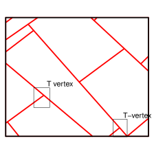
(c)

Figure 4: A fragment of the Selommes landscape transformed into a T-tessellation: (a) clusters of closed and aligned polygons sides; (b) tessellation spanned by representative segments; (c) tessellation after removal of the I- and L-vertices.

The distributions of three basic polygon characteristics in the Selommes landscape and its approximation are compared in Figure (5). The distributions of perimeter and area are similar before and after transformation. As for the number of vertices, its median value is comparable but the $75\%$ quantile and $95\%$ quantile are clearly higher in the original landscape. It is the effect of replacing closely aligned polygons sides in the original landscape by the representative segments in its approximation.

(a)

(b)

(c)

Figure 5: Distribution of the area, the perimeter and the number of vertices of polygons in the Selommes landscape and its approximation by a T-tessellation.

3 Gibbsian T-tessellation model

Let $\mathcal{T}$ denote a set of all T-tessellations of a bounded polygonal domain $W\subset\mathbb{R}^{2}$. Each tessellation $T\in\mathcal{T}$ can be defined by the union of the boundaries of its cells $\displaystyle E_{T}$, a closed set with an empty interior. Thus, we can define on $\mathcal{T}$ a standard hitting $\sigma$-algebra for the closed sets, generated by the events :

$$\mathcal{T}_{K}=\{T\in\mathcal{T}:\displaystyle E_{T}\cap K\neq\emptyset\}$$

for $K\in\mathbb{K}$, a set of all compact subsets of $W$ (see [20]). The corresponding measurable space will be denoted by $\{\mathcal{T},\sigma(\mathcal{T})\}$. It should be noted that we can assign to each tessellation $T\in\mathcal{T}$ a set of the lines supporting the segments of $T$. Conversely, we can assign to each line pattern $L$ intersecting $W$ the set of all T-tessellations supported by the lines of $L$. This observation leads us to a definition of a counting measure on $\sigma(\mathcal{T})$, corresponding to a line pattern $L$.

Definition 2.

Let $L$ be a line pattern intersecting a domain $W$ and let $\mathcal{T}(L)$ be a set of all T-tessellations supported by the lines of $L$. A measure $\mu_{L}$ on $\sigma(\mathcal{T})$ is defined as:

$$\mu_{L}(A)=\sum_{T\in\mathcal{T}(L)}\mathbb{I}_{A}(T)\text{ }\quad\forall A\in\sigma(T)$$ (2)

where $\mathbb{I}_{A}$ stands for an indicator function of a set $A$. The measure $\mu_{L}(A)$ counts the tessellations in $A$ supported by the lines of $L$. When $L$ is a realization of a Poisson line process, the following extension of the previous definition holds:

Definition 3.

Let $\mathbf{L}$ be a Poisson line process with unit intensity, restricted to $W$. A measure $\mu$ on $\sigma(T)$ is defined as follows:

$$\mu(A)=\frac{1}{z}\mathbb{E}\mu_{\mathbf{L}}(A)\text{ }\quad\forall A\in\sigma(T)$$ (3)

where $z=\mathbb{E}|\mathcal{T}(\mathbf{L})|$ is a normalizing constant.

The model defined by the probability distribution (3) was proposed in [10] and referred to as the Completely Random T-Tessellation Model (CRTT). The finiteness of measures (2) and (3) was proven in [9] and [10].

The CRTT model can be considered as a reference measure on $\{\mathcal{T},\sigma(\mathcal{T})\}$. Let $s(T)$ be a $d$-dimensional vector of tessellation statistics and let $\theta$ be a corresponding parameter vector belonging to a parametric space $\Theta\subset\mathbb{R}^{d}$. Let us assume that each component of $s$ can be written as the sum of local contributions of tessellation vertices, edges, cells or segments:

$$s_{i}(T)=\sum_{e\in{\cal{E}}(T)}f_{i}(e)$$ (4)

where ${\cal{E}}(T)$ denotes the set of tessellation elements and $i$ varies from $1$ to $d$. The model that favors the tessellations with high (resp. low) values of statistics $s_{i}(T)$ is given by the following density function w.r.t. the measure $\mu$:

$$p_{\theta}(T)=\frac{1}{c_{\theta}}\exp\left(-\sum_{j=1}^{d}\theta_{j}s_{j}(T)\right)$$ (5)

where $c_{\theta}$ is an unknown normalizing constant. The scalar product defining the probability density 5 is denoted by :

$$U_{\theta}(T)=\langle\theta,s(T)\rangle$$ (6)

Model (5) is referred as a Gibbs model for T-tessellations and the function $U_{\theta}(T)$ is the energy function of the model. Depending on the chosen statistics, the model makes it possible to control various T-tessellation features: cell area variability, angles between edges, etc.

Example 1.

Let us consider a Gibbs model with the following statistic :

$$s_{\sphericalangle}(T)=\sum_{c\in C(T)}\left(\sum_{v\in V(c)}\left(\frac{\pi}{2}-\alpha(v)\right)\right)$$ (7)

The first sum in (7) runs through a tessellation cells, denoted by $C(T)$. For each cell $c$, the set of its vertices $V(c)$ is considered in a second sum. The vertex $v$ contributes to the energy function only if the angle $\alpha(v)$ between the sides incident to $v$ is acute (see Figure 6). The contribution of a vertex $v$ is close to $0$ if the sides are almost perpendicular. Thus the statistic $s_{\sphericalangle}(T)$ measures a deviation of tessellation cells from rectangles.

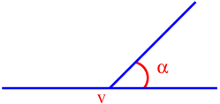
Figure 6: Acute angle between the edges incident to a vertex $v$.

A Metropolis-Hastings-Green algorithm for the simulation of the Gibbs model (5) was proposed and its convergence properties were discussed in ([10]). It is based on three local updates of a T-tessellation: a split of tessellation cell, a merge of two cells and a removal of an edge at the end of a blocking segment, followed by an insertion of an edge incident to a new endpoint of the shortened segment. The algorithm was implemented in the C++ library ([1]).

Figure (7) illustrates an example of the simulation of the CRTT model (2) and of the model with angle statistic $s_{\sphericalangle}(T)$.

(a)

(b)

Figure 7: Simulation of: (a) CRTT model (3); (b) Gibbs model with angle statistic (7).

3.1 MCML inference

Model parameters were estimated by Monte Carlo Maximum Likelihood method, proposed in [7] for the families of distributions specified by the unnormalized densities. The method relies on the possibility of sampling from the targeted distribution. For the Gibbs model, the log-likelihood ratio against a fixed point $\psi\in\Theta$ is defined as:

$$l(\theta|T,\psi)=\log\frac{p_{\theta}(T)}{p_{\psi}(T)}=U_{\psi}(T)-U_{\theta}(T)-\log\frac{c_{\theta}}{c_{\psi}}$$ (8)

This ratio depends on the ratio of unknown normalizing constants, which can be expressed as:

$$\frac{c_{\theta}}{c_{\psi}}=\mathbb{E}\exp\left(U_{\psi}(T)-U_{\theta}(T)\right)$$ (9)

when the expectation in (9) is calculated under the known distribution $P_{\psi}$. Let ${\bf T}_{n}=(T_{1},\ldots,T_{n})$ be a sample simulated from $P_{\psi}$. The expected value in (9) can be estimated by the empirical mean:

$$\frac{c_{\theta}}{c_{\psi}}\simeq\frac{1}{n}\sum_{i=1}^{n}\exp\left(U_{\psi}(T_{i})-U_{\theta}(T_{i})\right)$$ (10)

The estimate of the unknown log-likelihood ratio (8) is obtained by substituting the ratio of normalizing constants with its approximation (10). It is called a Monte Carlo Likelihood (MCL) function and denoted by $\hat{l}_{n}(\theta)$. The maximizer $\hat{\theta}_{n}$ of the MCL function approximates the unknown value of the Maximum Likelihood estimate $\hat{\theta}$. The asymptotic properties of $\hat{l}_{n}$ and $\hat{\theta}_{n}$ were derived in [6] and [13].

The likelihood of exponential family models is convex. Hence the optimization of its Monte Carlo approximation is justified. The method holds for every value of $\psi$, but in practice the choice of this parameter has an impact on the quality of the estimation. If $\psi$ is far from the exact estimate, MCL approximation is poor and $\hat{\theta}_{n}$ will be far from $\hat{\theta}$ as well. One possible solution to this problem is to iterate the optimization algorithm. The trust region method applied here for calculating $\hat{\theta}_{n}$ (see [4]) starts from an arbitrary parameter $\psi$ and maximizes quadratic approximation of $\hat{l}_{n}$ over a region $\Delta$ around $\psi$, yielding a new parameter value. The size of the region $\Delta$ is adjusted in order to obtain a correct approximation of $\hat{l}_{n}$ by a quadratic model.

Figure 8 illustrates the algorithm for calculating the estimates of a two-parameter model with an energy function:

$$U_{\theta}(T)=-\theta_{1}n_{s}(T)+\theta_{2}s_{\sphericalangle}(T)$$ (11)

where $n_{s}(T)$ is the number of internal segments of $T$ and $s_{\sphericalangle}(T)$ is the angle statistic already defined in example (1). The model was fitted to the tessellation $T_{0}$ simulated with parameter $\theta=(31,5)$ in the unit square (see Fig. 8a). The algorithm started from $\psi=(24,10)$ and reached the maximum after $12$ iterations. The calculation of a current value of the estimate was based on a Monte Carlo sample of size $400$. The distribution of two statistics calculated over $1000$ runs of the fitted model appears to be correctly centered on the observed values (see Fig. 8c).

(a)

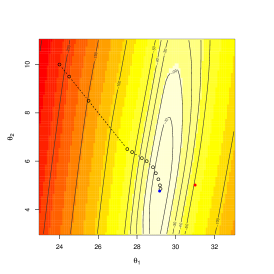
(b)

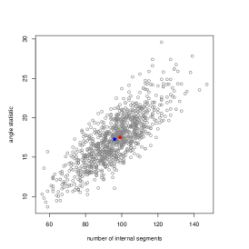
(c)

Figure 8: Estimation of parameters of the model (11). (a) Training tessellation $T_{0}$ simulated with $\theta=(31,5)$. (b) Contour plot of MCL function. The true parameter is represented by a red dot. The algorithm starts at $\psi=(24,10)$ and converges after $12$ iterations at $\hat{\theta}_{n}=(29.15,4.76)$ (blue dot). (c) Scatter plot of the values of energy statistics calculated for $1000$ simulations of the fitted model. The blue and the red dot represent respectively the mean and the observed values of the statistics.

The standard error of the Maximum Likelihood estimate $\hat{\theta}$ for model (11), calculated from the Monte Carlo approximation of the Fisher Information Matrix with $n=400$, was equal to $(0.0135,0.2900)$. The asymptotic results given by Geyer in ([6]) make it possible to estimate the standard error of the approximation $\hat{\theta}_{n}$, referred to as the Monte Carlo Standard Error (MCSE). Figure (9) shows the graphs of MCSE($\hat{\theta}_{n_{1}}$) and MCSE($\hat{\theta}_{n_{2}}$) as the sample size grows from $n=200$ to $n=1200$. The highest value of MCSE($\hat{\theta}_{n}$) was equal to $(0.000021,0.00016)$ for the sample size $n=200$. The MCSE($\hat{\theta}_{n}$) decreased rapidly as the sample size varied from $200$ to $600$. Beyond this threshold no significant improvement of the accuracy of $\hat{\theta}_{n}$ was observed.

(a)

(b)

Figure 9: Monte Carlo standard error of $\hat{\theta}_{n_{1}}$ (left panel) and $\hat{\theta}_{n_{2}}$ (right panel) as a function of sample size $n$.

4 Gibbs model for landscapes comparison and simulation

The epidemic models of plant diseases are studied at the landscape scale. Landscape features are likely to play a role in the epidemic spread, interacting with other variables determining the dynamics of the host-pathogen system. The impact of variables is evaluated through numerical experiments (see [16]). Landscape effect is measured by comparing the model’s outputs calculated for the landscapes contrasted with respect to the targeted features, like in factorial experiments. The design of such experiments requires a set of landscapes that differ with respect to the variables of interest. If the access to the landscape databases is somehow restricted, simulations of simplified landscape representations can be an alternative approach.

The Gibbs model can be a useful tool for yielding contrasted tessellation patterns that inherit the observed landscapes features. Let us illustrate this approach on the example of three landscapes in (2). The first step is to find out what the characteristics are that differ between the landscapes, fitting a guess model to landscape approximations and comparing the estimates of model parameters.

The guideline for choosing the model statistics is therefore their ability to capture the contrasts between the observed patterns. Based on these considerations, the candidate model with the following statistics was proposed first:

• the number of tessellation cells $s_{1}(T)$, accounting for the differences in tessellation scales;

• the sum of squared cell areas $s_{2}(T)$, measuring the departure from the patterns with cells with equal areas, minimizing the value of the statistic;

• the angle statistics $s_{3}(T)$, measuring the departure from orthogonal patterns. This statistic, already introduced in example (7), was renamed here so that all of the statistics would have a common notation;

• the number of long cells $s_{4}(T)$. A cell is said to be long if the length-to-width ratio of its smallest enclosing rectangle (see Fig. 10) is greater than a threshold $l_{0}$. In this case the value of $l_{0}$ was fixed at $4$, the value close to the median length-to-width ratio in the BVD landscape.

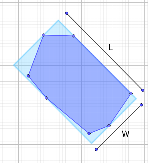
Figure 10: Length-to-width ratio of minimal bounding rectangle.

Let $T_{1}$, $T_{2}$ and $T_{3}$ be the observed tessellations, approximating the landscapes represented in Figure (2). Let a tessellation $T_{i}$ follow a Gibbsian model given by the energy:

$$U_{\theta_{i}}(T_{i})=\sum_{j=1}^{4}\theta_{i,j}s_{j}{(T_{i})}$$ (12)

for $i\in\{1,2,3\}$. Table (1) gives Monte Carlo Maximum Likelihood estimates of model parameters together with their $95\%$ confidence sets, based on the approximation of the Fisher Information Matrix inverse. The size of the Monte Carlo sample was fixed at $n=500$.

Landscape $T_{i}$	$\hat{\theta}_{i,1}$	$\hat{\theta}_{i,2}$	$\hat{\theta}_{i,3}$	$\hat{\theta}_{i,4}$
Selommes	-1.98	182	2.22	0.27
	(-2.23,-1.73)	(55,309)	(1.92,2.50)	(-0.05,0.61)
Kervidy	-1.69	80	1.26	0.05
	(-1.90,-1.49)	(-25,187)	(1.04, 1.48)	(-0.28,0.38)
BVD	-2.08	2518	2.18	-0.58
	(-2.32,-1.83)	(1217,3819)	(1.89,2.47)	(-0.83,-0.48)

Table 1: MCML estimates of the parameters of model (12) and their $95\%$-confidence sets.

The model fitted to the BVD landscape tends to generate the tessellations close to the patterns with equally sized cells (high positive value of $\hat{\theta}_{2}$) and orthogonal segments (positive value of $\hat{\theta}_{3}$).The model favors the patterns with a number of long cells greater than in other landscapes and greater than in the reference model (negative value of $\hat{\theta}_{4}$). The model fitted to the Kervidy landscape is closest to completely random T-tessellation. The estimates of parameters ${\theta}_{2}$ and ${\theta}_{4}$ are non-significantly different from zero. The penalty for the acute angles between the segments ($\hat{\theta}_{3}$) is positive, but its value is smaller than the estimates calculated for the Selommes and BVD landscapes. The model fitted to Selommes data generates the most rectangular patterns with the smallest number of long cells.

Figure (11) gives the examples of model simulations for the three landscapes. According to the model properties, the mean values of the statistics calculated over a sample of tessellations simulated from (12) are centered on the values observed in the landscapes. In this sense, the model is able to generate simplified landscape representations that inherit selected landscape features.

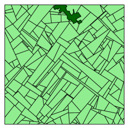
(a)

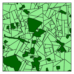
(b)

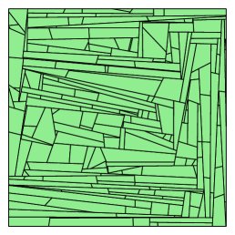
(c)

Figure 11: Simulations of Gibbs model (12) fitted to (a) Selommes, (b) Kervidy and (c) BVD landscapes.

4.1 Empty-space function for testing goodness-of-fit

The empty-space function $F$ is a summary statistic commonly applied in spatial point pattern analysis to characterize the observed patterns and to check point process model validity (see [3]). The function definition can be extended to the other random sets, e.g. line segments and linear networks (see [11], [5]). For a random stationary tessellation ${T}$, the empty-space function is defined as the cumulative distribution function of the shortest distance $d(u,T)$ from an arbitrary point $u$ in the tessellation domain to $T$:

$$F_{T}(r)=P(d(u,T)\leq r)$$ (13)

Since $T$ is stationary, the definition (13) does not depend on a particular choice of $u$. The function $F_{T}(r)$ can be interpreted as the average fraction of the area of the region obtained by the dilation of tessellation $T$ by a disc with a radius $r$. Consequently, for tessellations with cells that have regular shapes and sizes, such as grid patterns, $F_{T}$ will tend to grow more rapidly than, for example, in the CRTT model. The empty-space function is thus a useful tool for comparing the observed patterns between themselves or with the patterns generated by a candidate model. The border-corrected estimate of $F_{T}(r)$ is calculated over the points sampled in the tessellation domain and separated from the border by a distance greater than or equal to $r$:

$$\hat{F}_{T}(r)=\frac{\#\{u_{i}:d(u_{i},T)\leq r\cap d(u_{i},\partial W)\geq r\}}{\#\{u_{i}:d(u_{i},\partial W)\geq r\}}$$ (14)

where $\partial W$ denotes the border of the tessellation domain $W$ (see [5]).

The global envelope test for model checking compares a functional statistic of the observed pattern with its counterparts calculated for the simulations of the null model (see [14]). The test is applied for checking point process models, but its extension to random tessellation models is straightforward. The principle of the test procedure is to reduce a tessellation pattern $T$ to a random variable $X=X(T)$ and to compare the distribution of $X$ for the observed pattern with its distribution simulated from a null model. Let $X_{\text{obs}}$ denote the value of $X$ for the observed tessellation $T_{\text{obs}}$ and let $X_{1},\ldots,X_{m-1}$ be the values of $X$ calculated for a sample of tessellations $T_{1},\ldots,T_{m-1}$ generated by a null model. The tessellations $T_{1},\ldots,T_{m-1}$ are assumed to be independent of each other and independent of the observed pattern. Let $P_{x}$ denote the distribution of the i.i.d. sample $X_{1},\ldots,X_{m-1}$. A null hypothesis states that:

$$H_{0}:X_{\text{obs}}\sim P_{x}$$ (15)

Let $R_{\text{obs}}$ be the rank of $X_{\text{obs}}$ in a pulled sample $X_{\text{obs}},X_{1},\ldots,X_{m-1}$. Under the null hypothesis this is an i.i.d sample and the following equality holds:

$$P_{H_{0}}(R_{\text{obs}}>m-1)=\frac{1}{m}$$

Thus, if $X_{\text{obs}}$ is greater than a maximal value of $X_{i}$ than the null hypothesis (15) is rejected at a significance level $\alpha=\frac{1}{m}$.

The choice of the variable $X(T)$ is subject to the constraint that its large positive values are unlikely under a null hypothesis. Different variants of envelope test were proposed depending on the definition of $X(T)$ (see [3]). In the Maximum Absolute Deviation test based on the empty-space function, the variable $X(T)$ is defined as the maximal absolute difference between the estimate of $F_{T}$ and its expected value under the null hypothesis:

$$X(T)=\max_{0\leq r\leq R}|\hat{F}_{T}(r)-{F}_{\text{ref}}(r)|$$ (16)

The maximum in (16) is taken over a range of distances from $0$ to $R$ units. If ${F}_{\text{ref}}$ in formula (16) cannot be calculated explicitly, it can be estimated from the simulations of a null model. Testing the null hypothesis (15) with the MAD test is equivalent to checking if $\hat{F}$ calculated for the observed tessellation falls inside the interval:

$$\left({F}_{\text{ref}}(r)-\max_{i}X_{i},{F}_{\text{ref}}(r)+\max_{i}X_{i}\right)$$ (17)

for every $r$ in $(0,R)$. If this is the case, there is no evidence for rejecting $H_{0}$.

The test was applied to check the goodness-of-fit of model (12). Figure 12 shows the envelopes (17) based on $m-1=499$ model simulations. The estimated $F$-function for the observed patterns falls entirely inside the envelopes for each landscape. At the significance level $\alpha=\frac{1}{500}$ there is no evidence against the null hypothesis that landscape patterns follow the Gibbs model (12) with the parameters values given by Table (1). The corresponding p-values of the test are: $0.53$ for the Selommes, $0.38$ for the BVD and $0.20$ for the Kervidy landscape.

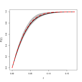
(a)

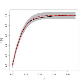
(b)

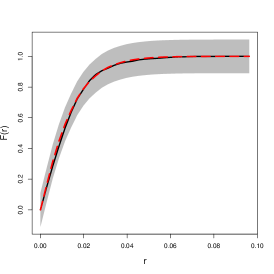
(c)

Figure 12: Simultaneous envelopes (17) for the empty-space function: (a) Selommes landscape; (b) Kervidy landscape; (c) BVD landscape. Estimates of the empty-space function for the observed patterns are plotted in black. The dashed red curves represent the estimates of $F_{\text{ref}}$ for model (12).

5 Conclusions

Random T-tessellations following the Gibbs model proposed in ([10]) may represent a broad scope of spatial patterns. This paper completes the model with a statistical inference tested on the example of agricultural landscapes, approximated by T-tessellations. The proposed landscape model highlights the differences between the observed patterns. Model parameters are estimated by the Monte Carlo Maximum Likelihood method. Confidence sets calculated from MC approximation of the Fisher Information Matrix enable parameters comparison. The goodness-of-fit of the model is assessed by the global envelope test for the empty-space function.

The framework of Monte Carlo Likelihood inference may give rise to the development of variable selection methods for the Gibbs model. Starting from a set of candidate variables, a stepwise procedure can be considered for variables inclusion and elimination, based on Monte Carlo approximation of Likelihood tests. From a practical view point it should be accompanied by the development of more efficient computational methods for finding $\hat{\theta}_{n}$. Indeed, the calculation of the estimate becomes cumbersome as the number of variables grows.

Strong correlations between the model statistics may be at the origin of the difficulties in model fit. The example of the model fitted to the BVD landscape illustrates this problem. The model accounts for a high number of long cells and, at the same time, favors the patterns with equally distributed cell areas. In order to satisfy both criteria the model tends to generate the cells with extremely elongated shapes, as illustrated in Figure (11). Consequently, the model alters the mean elongation of tessellation cells, making it difficult to fit the model while controlling the values of this statistic at the same time. The question of how to select a set of tessellation statistics to avoid correlation issues is of major interest for statistical inference.

Finally, the generalization of the model to polygonal tessellations with no restrictions on the vertices type would be of great practical interest as well. The source of bias due to the approximation of the original pattern by a T-tessellation could be avoided in this way.

References

- [1] K. Adamczyk-Chauvat and K. Kiêu. LiTe. http://kien-kieu.github.io/lite, 2015.
- [2] T. Arak, P. Clifford, and D. Surgailis. Point-based polygonal models for random graphs. Advances in Applied Probability, 25:348–372, 1993.
- [3] A. Baddeley, E. Rubak, and R. Turner. Spatial Point Patterns: Methodology and Applications with R. Chapman and Hall/CRC, 2016.
- [4] R. Fletcher. Practical Methods of Optimization, Second Edition. Wiley, 2000.
- [5] R. Foxall and A. Baddeley. Nonparametric measures of association between a spatial point process and a random set, with geological applications. Journal of the Royal Statistical Society, Series C, 51:165–182, 2002.
- [6] C.J. Geyer. On the convergence of Monte Carlo maximum likelihood calculations. Journal of the Royal Statistical Society, Series B, 56:261–274, 1994.
- [7] C.J. Geyer. Likelihood inference for spatial point processes. In O.E. Barndorff-Nielsen, W.S. Kendall, and M.N.M. van Lieshout, editors, Stochastic Geometry - Likelihood and Computation, volume 80 of Monographs on Statistics and Applied Probability, pages 79–140. Chapman and Hall/CRC, 1999.
- [8] E.N. Gilbert. Applications of Undergraduate Mathematics in Engineering, chapter Random plane networks and needle-shaped crystals. Noble, B., 1967.
- [9] J. Kahn. How many T-tessellations on k lines? existence of associated Gibbs measures on bounded convex domains. Random Structures & Algorithms, 47:561–587, 2015.
- [10] K. Kiêu, K. Adamczyk-Chauvat, H. Monod, and R.S. Stoica. A completely random T-tessellation model and Gibbsian extensions. Spatial Statistics, 6:118–138, 2013.
- [11] F.K. Klienschroth, J.R. Healey, F. Mortier, and R.S. Stoica. Effects of logging on roadless space in intact forest landscapes of the Congo Basin. Conservation Biology, 31:469–480, 2016.
- [12] M. Mackisack and R. Miles. Homogeneous rectangular tessellations. Advances in Applied Probability, 28:993–1013, 1996.
- [13] B. Miasojedow, W. Niemiro, J. Palczewski, and W. Rejchel. Asymptotics of Monte Carlo likelihood estimators. Probability and Mathematical Statistics, 36:295–310, 2016.
- [14] M. Myllymaki, T. Mrkvicka, P. Grabarnik, H. Seijo, and U. Hahn. Global envelope tests for spatial processes. Journal of the Royal Statistical Society, Series B, 79:381–404, 2017.
- [15] W. Nagel and V. Weiß. Crack STIT tessellations: Characterization of stationary random tessellations stable with respect to iteration. Advances in Applied Probability, 37:859–883, 2005.
- [16] J. Papaïx, K. Adamczyk-Chauvat, A. Bouvier, K. Kiêu, S. Touzeau, and C Lannou. Pathogen population dynamics in agricultural landscapes: the Ddal modelling framework. Infection, Genetics and Evolution, 27:509–520, 2014.
- [17] S. Pivard, K. Adamczyk, J. Lecomte, C. Lavigne, A. Bouvier, A. Deville, P.H. Gouyon, and S. Huet. Where do the ferail oilseed populations come from? A large-scale study of their possible origin in a farmland area. Journal of Applied Ecology, 45:476–485, 2008.
- [18] S. Poggi, A. Delaplace, P. Pichelin, and R. Le Cointe. History of land uses over the period 2013-2019 in the Kervidy-Naizin watershed (Brittany, France). https://doi.org/10.15454/ATYOBO, 2020.
- [19] B. Ricci, P. Franck, J.-F. Toubon, J.-C. Bouvier, B. Sauphanor, and C. Lavigne. The influence of landscape on insect pest dynamics: a case study in southeastern France. Landscape Ecology, 24:337–349, 2009.
- [20] D. Stoyan, W.S. Kendall, and J. Mecke. Stochastic geometry and its applications, Second edition. Wiley, 1996.