Flavor Hierarchies from Clockwork in $\boldmath{SO(10)}$ GUT

Abstract

The clockwork mechanism, which can naturally explain the origin of small numbers, is implemented in $SO(10)$ grand unified theories to address the origin of hierarchies in fermion masses and mixings. We show that a minimal Yukawa sector involving a $10_{H}$ and $\overline{126}_{H}$ of Higgs bosons, extended with two clockwork chains consisting of $16+\overline{16}$ vector-like fermions, can explain the hierarchical patterns with all the Yukawa couplings being of order one. Emergence of a realistic mass spectrum does not require any symmetry that distinguishes the three generations. We develop clockwork-extended $SO(10)$ GUTs both in the context of SUSY and non-SUSY frameworks. Implementation of the mechanism in non-SUSY scenario assumes a Peccei-Quinn symmetry realized at an intermediate scale, with the clockwork sector carrying non-trivial charges, which solves the strong CP problem and provides axion as a dark matter candidate.

1 Introduction

The origin of the observed hierarchies in the masses and mixings of quarks and leptons is a longstanding puzzle in the Standard Model (SM) of particle physics, commonly referred to as the flavor puzzle. Whereas the charged fermion masses and mixings appear to be strongly hierarchical between generations, in the neutrino sector only a mild hierarchy is realized. Additionally, a stronger hierarchy is observed in the up-quark mass ratios compared to the down-quark and charged lepton counterparts, which have very similar patterns. The SM fails to provide an explanation of the flavor puzzle as it simply accommodates the observed masses and mixings in terms of completely free Yukawa coupling parameters. Besides, neutrinos are strictly massless in the SM, which contradicts observations. There have been many attempts to address the flavor puzzle among which grand unified theories (GUTs) Pati:1974yy ; Georgi:1974sy ; Georgi:1974yf ; Georgi:1974my ; Fritzsch:1974nn based on $SO(10)$ gauge group Georgi:1974my ; Fritzsch:1974nn are very attractive candidates. In addition to unifying the strong, weak and electromagnetic forces into a single force, in $SO(10)$ GUTs, quarks and leptons of each family are unified into a single irreducible $16$-dimensional representation. Along with the SM fermions, this $16$-dimensional spinor representation contains the right-handed neutrino that naturally leads to small but non-zero neutrino masses via the seesaw mechanism Minkowski:1977sc ; Yanagida:1979as ; Glashow:1979nm ; GellMann:1980vs ; Mohapatra:1979ia . The unification of all fermions of a family into an irreducible representation is a good starting point to address the flavor puzzle, owing to the various correlation it provides. Further appealing features of this theory include a natural understanding of electric charge quantization, automatic anomaly cancellation, and gauge coupling unification at high energy scale around $10^{16}$ GeV with or without supersymmetry (SUSY).

Because of the unification of quarks and leptons of each family into a single irreducible representation, $SO(10)$ GUT is one of the best frameworks that can shed some light on the flavor puzzle. The Higgs fields that can generate fermion masses at the renormalizable level can be identified from the fermion bilinears

$$16\times 16=10_{s}+120_{a}+126_{s}\;,$$ (1.1)

where the subscripts $s$ and $a$ denote symmetric and antisymmetric flavor structures. A minimal Yukawa sector in SUSY $SO(10)$ GUT and/or non-SUSY $SO(10)$ with a $U(1)$ Peccei-Quinn (PQ) symmetry Peccei:1977hh consists of two Higgs multiplets $10_{H}$ and $\overline{126}_{H}$ having the following interactions Babu:1992ia :

$${\cal L}_{Y}=16^{T}\left(Y_{10}\,10_{H}+Y_{126}\overline{126}_{H}\,\right)16\;.$$ (1.2)

In the non-SUSY framework, the PQ symmetry would require complexification of the $10_{H}$. The complex conjugate of $10_{H}$ however, does not couple to fermions, owing to its PQ charge, thus preserving the form of Eq. (1.2). The flavor phenomenology would thus be similar in the SUSY version as well the PQ-symmetric non-SUSY version, with the Yukawa couplings given by Eq. (1.2) in both cases. Introduction of the PQ symmetry is of course highly motivated on independent grounds, since it naturally solves the strong CP problem and also provides a viable dark matter candidate in the axion.

The fermion mass matrices derived from the minimal Yukawa sector of Eq. (1.2) has only 19 real parameters (of which 7 are phases) to fit 19 observed quantities, making the theory very predictive in the flavor sector. These observed quantities are the 6 quark and 3 charged lepton masses; 2 neutrino mass-squared differences; 3 quark mixing angles; 3 lepton mixing angles; and 2 Dirac CP phases – 1 in the quark mixing matrix and 1 in the lepton mixing matrix. Since these parameters are all interrelated in $SO(10)$ and since they should fit different hierarchical patterns in the charged fermion and the neutral fermion sectors, finding an acceptable fit is a highly non-trivial task. This issue has been been extensively studied in the literature and the consistency of the minimal Yukawa sector established Babu:1992ia ; Bajc:2001fe ; Bajc:2002iw ; Fukuyama:2002ch ; Goh:2003sy ; Goh:2003hf ; Bertolini:2004eq ; Bertolini:2005qb ; Babu:2005ia ; Bertolini:2006pe ; Bajc:2008dc ; Joshipura:2011nn ; Altarelli:2013aqa ; Dueck:2013gca ; Fukuyama:2015kra ; Babu:2018tfi ; Babu:2018qca ; Ohlsson:2019sja . In particular, the reactor neutrino mixing angle $\theta_{13}$ was predicted to be large and close to its experimentally measured value. While the minimal Yukawa sector involving $10_{H}+126_{H}$ of Higgs fields is sufficient to explain observed data, a flavor-antisymmetric $120_{H}$ Yukawa coupling matrix could be added to Eq. (1.2) Dutta:2004hp ; Dutta:2005ni ; Lavoura:2006dv ; Ferreira:2015jpa ; Fukuyama:2016vgi ; Babu:2016bmy ; Deppisch:2018flu . Although the clockwork mechanism we develop here can be straightforwardly extended to this non-minimal case, we do not purse it here.

While achieving good fits to the fermion masses and mixings with the minimal Yukawa sector is certainly a great success for $SO(10)$ GUT, this framework does not explain the hierarchical features observed in the spectrum. One idea that has been pursued to explain the hierarchy is to use additional symmetries that distinguish families which can lead to highly regulated fermion mass matrices (for reviews see Refs. Babu:2009fd ; Feruglio:2015jfa ; Xing:2019vks and references therein). In such attempts, typically, the vacuum expectation values (VEVs) of certain flavon fields which break the flavor symmetry have to be arranged in a preferred pattern, which may not be entirely satisfactory. Another widely used approach is the implementation of the Froggatt-Nielsen mechanism Froggatt:1978nt with a flavor-dependent $U(1)$ symmetry wherein lighter fermion masses arise as higher dimensional operators, which are thereby naturally suppressed. While the coefficients of the higher dimensional operators can all be of order one, being non-renormalizable in nature, this setup does not provide quantitative predictions.

Recently, an interesting mechanism dubbed as the clockwork mechanism has been proposed Choi:2015fiu ; Kaplan:2015fuy to explain small numbers. While the initial motivation was to explain the gauge hierarchy problem in the context of relaxions, this mechanism has been generalized for broader model building purposes in Ref. Giudice:2016yja . The clockwork mechanism is an economical and elegant way to naturally generate large hierarchies between different quantities within a theory that contains only $\mathcal{O}(1)$ couplings. Briefly, this mechanism when applied to the flavor puzzle works as follows. The SM is enlarged with $N$ fermions that are vector-like under the SM which may be viewed as a one dimensional lattice. Due to an enforced symmetry, only nearest-neighbor interactions are allowed among the lattice sites, and only along one direction. Upon integrating out these heavy states on the lattice, hierarchy factors are generated – which may be even exponential for large number of lattice sites – via a sharp localization of the zero mode (the SM fermion) towards the boundary of the lattice. This idea can be readily extended to $3\times 3$ matrices in flavor space to create inter-generational hierarchies. For implementation of the clockwork mechanism to address flavor puzzle in various contexts see Refs. vonGersdorff:2017iym ; Patel:2017pct ; Alonso:2018bcg ; Sannino:2019sch ; Smolkovic:2019jow ; deSouza:2019wji ; vonGersdorff:2020ods , and for attempts to generate small neutrino masses and mixings see Refs.  Ibarra:2017tju ; Banerjee:2018grm ; Hong:2019bki ; Kitabayashi:2019qvi ; Kitabayashi:2020cpo . In Refs. vonGersdorff:2017iym ; Patel:2017pct ; Alonso:2018bcg ; Smolkovic:2019jow ; deSouza:2019wji , clockwork mechanism was incorporated into the SM flavour sector by introducing a set of vector-like fermions, where the number of added vector-like particles for each sector (up-type quark, down-type quark, and charged lepton) controls the pattern of the hierarchy for that particular sector. Ref. Alonso:2018bcg focused on TeV scale clockwork states, where a detailed phenomenology of vector-like fermions is also presented. Moreover, in Ref. Smolkovic:2019jow , two anomaly free versions of clockwork models with $U(1)$ and $[U(1)]^{3}$ flavor symmetries are presented to explain the observed hierarchies in the flavor sector. By allowing Yukawa couplings of the vector-like states with the Higgs fields that break the GUT symmetry, in Ref. vonGersdorff:2020ods flavor hierarchies are addressed in the context of $SU(5)$ and $SO(10)$ GUTs in the SUSY framework. Furthermore, by adding a set of SM singlet fermion states, flavor structures in the neutrino spectrum are analyzed in Ref. Ibarra:2017tju ; Hong:2019bki ; Kitabayashi:2019qvi . The observed flavor structure for the neutrino mass matrix with scalar clockwork has been implemented in Refs.  Banerjee:2018grm ; Kitabayashi:2020cpo .

In this work we present an interesting explanation to the flavor puzzle by combining the minimal Yukawa sector of $SO(10)$ GUT, Eq. (1.2), with clockwork mechanism. Within our framework, the GUT symmetry relates different flavors, whereas clockwork chains assist in providing the required hierarchical patterns. Thus the predictivity of the minimal Yukawa sector is preserved, while the origin of the small numbers obtained in the fit to fermion masses is also explained. In our construction, we introduce two clockwork chains consisting of $16+\overline{16}$ vector-like fermions, with all three families coupling to these clockwork chains indistinguishably. The longer of the two chains is responsible for generating small masses for the first generation fermions, while the shorter chain produces the required hierarchy for the second generation. While the clockwork mechanism has been applied separately to address quark flavor puzzle and neutrino masses and mixings, here we attempt a unified description involving both, which occurs naturally in grand unified theories, as in the minimal Yukawa sector of Eq. (1.2).

The rest of the paper is organized as follow. In Sec. 2 we show how to consistently implement clockwork mechanism in $SO(10)$ GUTs with the minimal Yukawa sector. In Sec. 3, we build complete models for both the SUSY and non-SUSY $SO(10)$ scenarios. In Sec. 4 we perform a numerical analysis of the complete fermion spectrum and demonstrate the predictivity of the setup. Finally, we conclude in Sec. 5. Two Appendices contains some technical details.

2 Clockwork $SO(10)$: Setup and formalism

In this section, we develop a clockwork extended $SO(10)$ GUT framework, which is equally applicable to scenarios with or without SUSY. In the latter case, a Peccei-Quinn symmetry plays the role that holomorphy of the superpotential plays in the case of SUSY. The Yukawa sector of the minimal renormalizable $SO(10)$ GUT Aulakh:1982sw ; Clark:1982ai ; Aulakh:2003kg ; Bajc:2004xe consists of $10_{H}$ and $\overline{126}_{H}$ Higgs multiplets that interact with the three generations of fermions $16_{i}$ ($i=1,2,3$) leading to the Yukawa interactions written in Eq. (1.2). To address the origin of hierarchical structure, we introduce a clockwork sector that consists of two sets of vector-like fermions in the $16+\overline{16}$ representations. One such clockwork chain consists of $n_{1}$ vector-like pairs $\chi_{a}+\overline{\chi}_{a}$ ($a=1,...,n_{1}$) charged under a $U(1)_{1}$ symmetry. The second clockwork chain contains $n_{2}$ vector-like pairs $\psi_{b}+\overline{\psi}_{b}$ ($b=1,...,n_{2}$) charged under a separate $U(1)_{2}$ symmetry. These abelian symmetries are broken by the VEVs of two separate scalar fields (flavons) $\phi_{1}$ and $\phi_{2}$ that are singlets of $SO(10)$ group. The $U(1)_{1}\times U(1)_{2}$ charges of all particles involved in the fermion mass generation are listed in Table I. Although the $U(1)$ symmetries may be taken to be global, the charge assignments are anomaly-free, and therefore the $U(1)$s can be identified as true gauge symmetries, which is what we shall adopt here.

$16_{i}$ $10_{H}$ $\overline{126}_{H}$ $\chi_{a}\;(16)$ $\overline{\chi}_{a}\;(\overline{16})$ $\psi_{b}\;(16)$ $\overline{\psi}_{b}\;(\overline{16})$ $\phi_{1}\;(1)$ $\phi_{2}\;(1)$ $U(1)_{1}\times U(1)_{2}$ $(0,0)$ $(0,0)$ $(0,0)$ $(+a,0)$ $(-a,0)$ $(0,+b)$ $(0,-b)$ $(+1,0)$ $(0,+1)$

Table I: Charges of the fields relevant for fermion mass generation under $U(1)_{1}\times U(1)_{2}$ symmetry.

Then the most general Yakawa interactions consistent with the $U(1)_{1}\times U(1)_{2}$ symmetry are given by

$$\mathcal{L}_{Y} =16^{T}_{i}\left(Y^{ij}_{10}\,10_{H}+Y^{ij}_{126}\overline{126}_{H}\,\right)16_{j}+\sum_{a=1}^{n_{1}}M_{a}\;\chi_{a}\overline{\chi}_{a}+\sum_{b=1}^{n_{2}}\overline{M}_{b}\;\psi_{b}\overline{\psi}_{b}$$

$$+\sum_{a=2}^{n_{1}}y_{a}\;\phi_{1}\;\chi_{a-1}\overline{\chi}_{a}+\sum_{b=2}^{n_{2}}\overline{y}_{b}\;\phi_{2}\;\psi_{b-1}\overline{\psi}_{b}+\phi_{1}\;\alpha_{i}\;16_{i}\;\overline{\chi}_{1}+\phi_{2}\;\beta_{i}\;16_{i}\;\overline{\psi}_{1}\;.$$ (2.3)

Note the interesting fact that all three generations of $16_{i}$ fermions couple to the clockwork chains indistinguishably. We shall see that a hierarchical structure will arise even in this case. Now, without loss of generality by making rotations in the flavor space one can bring the vectors $\alpha_{i}$ and $\beta_{i}$ to the following forms:

$$\alpha=(\alpha_{1},0,0),\;\;\;\beta=(\beta_{1},\beta_{2},0).$$ (2.4)

Furthermore, for the sake of simplicity, we assume universal coupling strength along each chain that are taken to be real, and define the following quantities

$$M_{a}=M_{1},\;\;\alpha_{1}\langle\phi_{1}\rangle=y_{a}\langle\phi_{1}\rangle\equiv-q_{1}M_{1},$$ (2.5)

$$\overline{M}_{b}=M_{2},\;\;\beta_{2}\langle\phi_{2}\rangle=\overline{y}_{b}\langle\phi_{2}\rangle\equiv-q_{2}M_{2},\;\;\beta_{1}\langle\phi_{2}\rangle\equiv-q_{3}M_{2}.$$ (2.6)

Note that with this choice, $\beta_{1}$ is the only term that couples the two clockwork chains.We first discuss a scenario where the two clockwork chains are decoupled, with $\beta_{1}=0$, and later present the most general analysis with $\beta_{1}\neq 0$. A schematic diagram to understand our proposed clockwork mechanism in $SO(10)$ GUT is presented in Fig. 1.

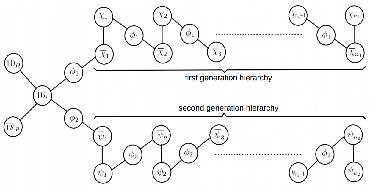
Figure 1: Schematic diagram for the clockwork mechanism in the proposed $SO(10)$ GUT. Solid lines correspond to the interactions present in the theory. Dotted lines represent the repetition of the clockwork chains.

2.1 Case with $\beta_{1}=0$

First we analyse the decoupled scenario of the two different clockwork chains that corresponds to $\beta_{1}=0$. In this simplified version of the theory, Eq. (2.3) takes the following simple form:

$$\mathcal{L}_{Y}=16^{T}_{i}\left(Y^{ij}_{10}\,10_{H}+Y^{ij}_{126}\overline{126}_{H}\;\right)16_{j} +M_{1}\sum_{a=1}^{n_{1}}\left(\chi_{a}\overline{\chi}_{a}-q_{1}\;\chi_{a-1}\overline{\chi}_{a}\right)+M_{2}\sum_{b=1}^{n_{2}}\left(\psi_{b}\overline{\psi}_{b}-q_{2}\;\psi_{b-1}\overline{\psi}_{b}\right).$$ (2.7)

In the above Yukawa interactions, the only two fermions $16_{1}$ and $16_{2}$ that directly couple to $10_{H}$ and $\overline{126}_{H}$ Higges, we denote them by $\chi_{0}$ and $\psi_{0}$, respectively. First consider the chain associated to $\chi$ fields. The corresponding mass matrix written in a basis $\overline{\chi}\mathcal{M}_{\chi}\chi$ with $\overline{\chi}=\left(\overline{\chi}_{1},...,\overline{\chi}_{n_{1}}\right)$ and $\chi=\left(\chi_{0},\chi_{1},...,\chi_{n_{1}}\right)^{T}$ has the following form:

$$\mathcal{M}_{\chi}=U\mathcal{M}^{diag}_{\chi}V^{T}=M_{1}\begin{pmatrix}-q_{1}&1&0&\cdots&&0\cr 0&-q_{1}&1&\cdots&&0\cr 0&0&-q_{1}&\cdots&&0\cr\vdots&\vdots&\vdots&\ddots&&\vdots\cr 0&0&0&\cdots&-q_{1}&1\end{pmatrix}_{n_{1}\times(n_{1}+1)}\;.$$ (2.8)

The above matrix is digonalized by the $U$ and $V$ matrices that are unitary. The eigenvalues of this matrix, including one zero mode and $n_{1}$ non-zero states are given by book

$$m^{2}_{0}=0;\;\;m^{2}_{a}=M_{1}^{2}\left(1+q_{1}^{2}-2q_{1}\cos\left[\frac{a\pi}{n_{1}+1}\right]\right);\;\;a=1,...,n_{1}.$$ (2.9)

We are interested in cases with $q_{i}\gtrsim\mathcal{O}(1)$; then the mass gap between two consecutive states is of order $\mathcal{O}(M_{i})$ as can be seen from Eq. (2.9). The analysis performed in this section is very general, and thus we need not specify the mass scale of the vector-like fermions. We will discuss this in more detail in the next section where we present complete models. The $n_{1}\times n_{1}$ unitary matrix $U$ has elements given by book

$$U_{ja}=-\sqrt{\frac{2}{n_{1}+1}}\sin\left[\frac{(n_{1}-j+1)\pi}{n_{1}+1}\right];\;\;j,a=1,...,n_{1}.$$ (2.10)

Furthermore, the elements of the $(n_{1}+1)\times(n_{1}+1)$ unitary matrix $V$ are as follows book :

$$V_{j0}=\sqrt{\frac{q_{1}^{2}-1}{q_{1}^{2}-q_{1}^{-2n_{1}}}}\;q_{1}^{j-n_{1}};\;\;j=0,....,n_{1},\;a=1,...,n_{1},$$ (2.11)

$$V_{ja}=\sqrt{\frac{2}{n_{1}+1}\frac{M^{2}}{m^{2}_{a}}}\left(q_{1}\sin\left[\frac{(n_{1}-j)a\pi}{n_{1}+1}\right]-\sin\left[\frac{(n_{1}-j+1)a\pi}{n_{1}+1}\right]\right).$$ (2.12)

From Eq. (2.11), it is clear that the massless mode is $\chi^{\prime}_{0}\equiv\hat{16}_{1}$ and that the only field $\chi_{0}\equiv 16_{1}$ that coupled originally to the SM Higgs in Eq. (2.7) (contained in the first two terms) are related by

$$16_{1}=V_{00}\hat{16}_{1}+\cdots$$

$$=\hat{16}_{1}\;\sqrt{\frac{q_{1}^{2}-1}{q_{1}^{2}-q_{1}^{-2n_{1}}}}\;\frac{1}{q_{1}^{n_{1}}}\equiv{\color[rgb]{1,0,0}\epsilon_{1}}\;\hat{16}_{1}.$$ (2.13)

Here $\cdots$ in the first line represents additional contributions from the heavy fields, which for our purpose are not important, and thus omitted in the next line. Since the SM fermions are contained in the zero-modes, the above equation demonstrates that the corresponding Yukawa couplings will have a suppression factor of order ${\color[rgb]{1,0,0}\epsilon_{1}}$ associated with the first generation fermions for $q_{1}>1$. This suppression can even be exponential, provided that $q_{1},n_{1}\gg 1$, although to explain flavor hierarchy these numbers need to be only somewhat larger than 1.

By repeating the whole process for the second decoupled chain containing $\psi$ fields, one obtains a similar expression for the massless mode $\psi^{\prime}_{0}\equiv\hat{16}_{2}$ and the original field $\psi_{0}\equiv 16_{2}$

$$16_{2}=\hat{16}_{2}\;\sqrt{\frac{q_{2}^{2}-1}{q_{2}^{2}-q_{2}^{-2n_{2}}}}\;\frac{1}{q_{2}^{n_{2}}}\equiv{\color[rgb]{0,0,1}\epsilon_{2}}\;\hat{16}_{2}.$$ (2.14)

Hence the Yukawa couplings associated with the second generation fermions receive a suppression of order ${\color[rgb]{0,0,1}\epsilon_{2}}\ll 1$ provided that $q_{2}>1$. These suppression factors are the origin of the fermion mass hierarchies. Assuming both $q_{1}$ and $q_{2}$ not very much larger than 1, the length of the clockwork chain associated with $\chi$ fields is required to be longer than the corresponding chain with the $\psi$ fields in order to generate the correct mass hierarchy between the first and the second families. Thus we choose $n_{1}>n_{2}$.

Now, integrating out the heavy fields and making use of Eqs. (2.13) and (2.14), we obtain for the light fermion Yukawa couplings as

$$\mathcal{L}_{Y} =\hat{16}^{T}\Lambda^{T}\;\left(Y_{10}\,10_{H}+Y_{126}\overline{126}_{H}\,\right)\;\Lambda\;\hat{16},\;\;~{}~{}~{}~{}~{}~{}~{}{\rm where}~{}~{}~{}\Lambda=\begin{pmatrix}{\color[rgb]{1,0,0}\epsilon_{1}}&&\\ &{\color[rgb]{0,0,1}\epsilon_{2}}&\\ &&1\end{pmatrix},$$ (2.15)

with $\hat{16}=\left(\hat{16}_{1}\;\hat{16}_{2}\;\hat{16}_{3}\right)^{T}$ and where the obvious identification $\hat{16}_{3}=16_{3}$ has been made. This $\Lambda$ matrix entering from the clockwork sector is the origin behind the observed hierarchical pattern of the fermion masses and mixings. This analysis shows that the Yukawa sector of the theory has the same number of parameters as in the minimal $SO(10)$ model, but with the couplings $Y^{ij}_{10},\,Y^{ij}_{126}$ being of order one. The mass and mixing hierarchies arise from the clockwork chains. The re-definitions $Y_{10}\rightarrow\Lambda^{T}Y_{10}\Lambda$ and $Y_{126}\rightarrow\Lambda^{T}Y_{126}\Lambda$ shows that the parameter count remains the same as in Eq. (1.2). For the convenience of the reader, we display the modified form of the Yukawa couplings explicitly:

$$\Lambda^{T}Y_{k}\Lambda=\begin{pmatrix}Y^{11}_{k}\;{\color[rgb]{1,0,0}\epsilon_{1}^{2}}&Y^{12}_{k}\;{\color[rgb]{1,0,0}\epsilon_{1}}{\color[rgb]{0,0,1}\epsilon_{2}}&Y^{13}_{k}\;{\color[rgb]{1,0,0}\epsilon_{1}}&\\ Y^{12}_{k}\;{\color[rgb]{1,0,0}\epsilon_{1}}{\color[rgb]{0,0,1}\epsilon_{2}}&Y^{22}_{k}\;{\color[rgb]{0,0,1}\epsilon_{2}^{2}}&Y^{23}_{k}\;{\color[rgb]{0,0,1}\epsilon_{2}}&\\ Y^{13}_{k}\;{\color[rgb]{1,0,0}\epsilon_{1}}&Y^{23}_{k}\;{\color[rgb]{0,0,1}\epsilon_{2}}&Y^{13}_{k}&\end{pmatrix},\;\;Y^{ij}_{k}\sim\mathcal{O}(1),\;\;k=10,\;126.$$ (2.16)

As will be detailed in Sec. 4, the minimal Yukawa couplings of $SO(10)$ that reproduce the correct masses and mixings for both the charged fermions as well as the neutrinos have the unique hierarchical structure as that of Eq. (2.16), which we will utilize for our numerical study. In Sec. 4, we perform a numerical analysis of the fermion masses and mixings and present our results for the down-quark and up-quark mass matrices in Eqs. (4.47) - (4.48) and in Eqs. (4.50) - (4.51) for SUSY and non-SUSY scenarios, respectively.

2.2 Case with $\beta_{1}\neq 0$

Generically, the term $\beta_{1}$ in Eq. (2.4) is non-zero. In this section, we discuss this general case and consider the following Yukawa interactions:

$$\mathcal{L}_{Y} =16^{T}_{i}\left(Y^{ij}_{10}\,10_{H}+Y^{ij}_{126}\overline{126}_{H}\,\right)16_{j}+M_{1}\sum_{a=1}^{n_{1}}\left(\chi_{a}\overline{\chi}_{a}-q_{1}\;\chi_{a-1}\overline{\chi}_{a}\right)$$

$$+M_{2}\sum_{b=1}^{n_{2}}\left(\psi_{b}\overline{\psi}_{b}-q_{2}\;\psi_{b-1}\overline{\psi}_{b}\right)-q_{3}M_{2}\chi_{0}\overline{\psi}_{1}\;.$$ (2.17)

Compared to Eq. (2.7), the newly added term is the very last entry in Eq. (2.17). This is the only term that couples the two clockwork chains, due to which, in this section we will follow a different method to compute the effective Yukawa Lagrangian. As before, we are interested in finding the overlap of the massless modes ($\hat{16}_{i}$) with the $0$-th site ($16_{i}$), which we achieve by integrating out heavy fields one-by-one as discussed below. Integrating out fermions at the $p$-th site leads to the following relation, which shows the overlap of the $p$-th site with the $(p-1)$-th site:

$$\begin{pmatrix}\chi_{p}\\ \psi_{p}\end{pmatrix}=L_{p}\begin{pmatrix}\chi_{p-1}\\ \psi_{p-1}\end{pmatrix}.$$ (2.18)

This way of integrating out the heavy states is convenient for our purpose, however, unlike the previous section, these transformation matrices $L_{p}$ are non-unitary. As a result, they modify the kinetic terms, which need to be brought back to the canonical form as done below.

Since we are interested in the scenario with $n_{1}>n_{2}$, $L_{p}$ appearing in Eq. (2.18) has the form

$$L_{p}=\begin{cases}\begin{pmatrix}q_{1}&0\\ q_{3}&q_{2}\end{pmatrix};\;\;p=1.\\ \begin{pmatrix}q_{1}&0\\ 0&q_{2}\end{pmatrix};\;\;p=2,3,...,n_{2}.\\ q_{1};\;\;p=n_{2}+1,...,n_{1}.\end{cases}$$ (2.19)

By applying the above definitions, we find the overlap between the $0$-th and the last site as

$$\begin{pmatrix}\chi_{0}\\ \psi_{0}\\ 16_{3}\end{pmatrix}=\left(Q_{n}...Q_{2}Q_{1}\right)^{-1}\begin{pmatrix}\chi_{n_{1}}\\ \psi_{n_{2}}\\ 16_{3}\end{pmatrix}.$$ (2.20)

Recall that associated with the third generation, there is no clockwork chain, and furthermore $n_{1}>n_{2}$. With these conditions, the $3\times 3$ matrices $Q_{p}$ of Eq. (2.20) are found to be

$$Q_{p}=\begin{cases}\begin{pmatrix}L_{p}&0\\ 0&1\end{pmatrix};\;\;p=1,2,...,n_{2}.\\ \begin{pmatrix}L_{p}&0\\ 0&\mathcal{I}_{2\times 2}\end{pmatrix};\;\;p=n_{2}+1,...,n_{1}.\end{cases}$$ (2.21)

This way of integrating out the clockwork fields modifies the kinetic terms that take the following form:

$$K\supset\sum_{p=0}^{n_{1}}\begin{pmatrix}\chi_{p}&\psi_{p}&16_{3}\end{pmatrix}^{\dagger}\not{D}\begin{pmatrix}\chi_{p}\\ \psi_{p}\\ 16_{3}\end{pmatrix}=\begin{pmatrix}\chi_{n_{1}}&\psi_{n_{2}}&16_{3}\end{pmatrix}^{\dagger}\not{D}Z\begin{pmatrix}\chi_{n_{1}}\\ \psi_{n_{2}}\\ 16_{3}\end{pmatrix}\;,$$ (2.22)

where we have defined

$$Z=\mathcal{I}_{3\times 3}+\left(P^{-1}_{n}\right)^{\dagger}\left(P^{-1}_{n}\right)+...+\left(P^{-1}_{1}P^{-1}_{2}...P^{-1}_{n}\right)^{\dagger}\left(P^{-1}_{1}P^{-1}_{2}...P^{-1}_{n}\right).$$ (2.23)

$$P^{-1}_{p}=\begin{cases}\begin{pmatrix}L_{p}^{-1}&0\\ 0&0\end{pmatrix};\;\;p=1,2,...,n_{2}.\\ \begin{pmatrix}L_{p}^{-1}&0\\ 0&0_{2\times 2}\end{pmatrix};\;\;p=n_{2}+1,...,n_{1}.\end{cases}$$ (2.24)

Then canonical normalization of the kinetic terms given in Eq. (2.22) along with Eq. (2.20) provides the desired relation:

$$\begin{pmatrix}\chi_{0}\\ \psi_{0}\\ 16_{3}\end{pmatrix}=\left(Q_{n}...Q_{2}Q_{1}\right)^{-1}Z^{-1/2}\begin{pmatrix}\hat{16}_{1}\\ \hat{16}_{2}\\ \hat{16}_{3}\end{pmatrix}=\Lambda\begin{pmatrix}\hat{16}_{1}\\ \hat{16}_{2}\\ \hat{16}_{3}\end{pmatrix}.$$ (2.25)

More explicitly, the suppression factors that originate from the clockwork sector are embedded in the matrix $\Lambda$ given by

$$\Lambda =\left(Q_{n}...Q_{2}Q_{1}\right)^{-1}Z^{-1/2}$$ (2.26)

$$=\begin{pmatrix}q_{1}^{-n_{1}}&0&0\\ -\frac{q_{3}}{q_{2}}q_{1}^{-n_{1}}&{q_{2}}^{-n_{2}}&0\\ 0&0&1\end{pmatrix}\begin{pmatrix}\frac{q_{1}^{2}-q_{1}^{-2n_{1}}}{q_{1}^{2}-1}&0&0\\ -\frac{q_{3}}{q_{2}}q_{1}^{-2n_{1}}&\frac{{q_{2}}^{2}-{q_{2}}^{-2n_{2}}}{{q_{2}}^{2}-1}&0\\ 0&0&1\end{pmatrix}^{-1/2}$$ (2.27)

$$=\begin{pmatrix}q_{1}^{-n_{1}}&0&0\\ -\frac{q_{3}}{q_{2}}q_{1}^{-n_{1}}&{q_{2}}^{-n_{2}}&0\\ 0&0&1\end{pmatrix}K_{1}\begin{pmatrix}\lambda_{1}^{-1/2}&0&0\\ 0&\lambda_{2}^{-1/2}&0\\ 0&0&1\end{pmatrix}K_{2}^{T}$$ (2.28)

$$\equiv\begin{pmatrix}\epsilon_{11}&\epsilon_{12}&0\\ \epsilon_{21}&\epsilon_{22}&0\\ 0&0&1\end{pmatrix}.$$ (2.29)

The matrices $K_{1,2}$ as well as the eigenvalues $\lambda_{1,2}$ are defined in Appendix A. As can be seen from Eq. (2.27), with $q_{3}=0$ (corresponding to two decoupled chains), one reproduces Eqs. (2.13) and (2.14).

3 Model implementation

In Sec. 2, we have discussed the clockwork implementation of the minimal Yukawa sector of $SO(10)$ without being specific to the theory being supersymmetric or not. In this section, we provide the necessary details to implement the mechanism in complete models with and without SUSY.

3.1 SUSY $SO(10)$ model

In minimal SUSY $SO(10)$ GUT, in addition to $10_{H}$ and $\overline{126}_{H}$, a $210_{H}$ Higgs representation is employed to consistently break the GUT symmetry in the SUSY limit. Proton decay constraints require the GUT symmetry breaking scale to be around $M_{GUT}\sim 10^{16}$ GeV, which is also the scale where the gauge couplings unify in the minimal supersymmetric standard model (MSSM). On the other hand, to generate viable light neutrino masses via type-I seesaw mechanism, the right-handed neutrinos must have masses which are a few orders smaller than the GUT scale, requiring $v_{R}\sim 10^{12}-10^{13}$ GeV ($v_{R}$ is the VEV of the SM singlet component of $126_{H}$). In this minimal setup, such a low value of $v_{R}$ would lead to certain colored states from the $126_{H}$ acquiring intermediate scale masses, thus spoiling perturbative gauge coupling unification Bertolini:2006pe ; Aulakh:2005bd ; Bajc:2005qe .

A simple choice to solve this issues is to introduce a $54_{H}$ Higgs multiplet Babu:2018tfi , which can break $SO(10)$ down to $SU(4)_{c}\times SU(2)_{L}\times SU(2)_{R}$ symmetry. It also supplies GUT scale masses to the would-be light colored states. Since $54_{H}$ has no couplings to fermion bilinears, the minimal Yukawa sector of Eq. (1.2) remains intact, which is our foucs here.

The $210_{H}$ can have renormalizable couplings with the fermions belonging to the clockwork sector of the form $\chi_{a}\overline{\chi}_{a}\;210_{H}$ (and similarly $\psi_{b}\overline{\psi}_{b}\;210_{H}$). The presence of these terms would introduce some modifications to the analysis performed in the previous section. This can be easily avoided by imposing a $\mathcal{Z}_{4}$ discrete symmetry. The full charge assignment that can do the job is presented in Table. II. Note that with this charge assignment the bare mass terms of the vector-like fermions would break the $\mathcal{Z}_{4}$ to a $\mathcal{Z}_{2}$. Alternatively, the VEV of a flavon field carrying -2 units of $Z_{4}$ charge break $\mathcal{Z}_{4}$ spontaneously to $\mathcal{Z}_{2}$.

$16_{i}$ $10_{H}$ $\overline{126}_{H}$ $210_{H}$ $\chi_{a}\;(16)$ $\overline{\chi}_{a}\;(\overline{16})$ $\psi_{b}\;(16)$ $\overline{\psi}_{a}\;(\overline{16})$ $\phi_{1}\;(1)$ $\phi_{2}\;(1)$ $\mathcal{Z}_{4}$ +1 -2 -2 0 +1 +1 +1 +1 -2 -2 $U(1)_{1}\times U(1)_{2}$ $(0,0)$ $(0,0)$ $(0,0)$ $(0,0)$ $(+a,0)$ $(-a,0)$ $(0,+b)$ $(0,-b)$ $(+1,0)$ $(0,+1)$

Table II: Charges of the particle of SUSY $SO(10)$ model with the imposition of a $\mathcal{Z}_{4}$ symmetry. Here $\mathcal{Z}_{4}$ charges are defined such that $\omega^{q_{4}}=1$ for $q_{4}=4$, where $\omega=e^{i2\pi/4}$. The model also contains $\overline{\phi}_{1}$ and $\overline{\phi}_{2}$ fields with charges opposite to those of $\phi_{1,2}$.

In this set-up with the $\mathcal{Z}_{4}$ symmetry, for our numerical study presented later in the text, we shall consider a case with $n_{1}=4$ and $n_{2}=2$. The mass scale of these vector-like fermions will be taken to be above the GUT scale. Consequently, the successful perturbative gauge coupling unification of MSSM would remain intact Dimopoulos:1981yj ; Ibanez:1981yh ; Einhorn:1981sx ; Marciano:1981un .

3.1.1 Symmetry breaking of $U(1)_{i}$

In this subsection, we discuss the symmetry breaking of $U(1)_{i}$ under which only the clockwork fields carry non-zero charges. We follow the method developed in Ref. Fayet:1974pd ; Fayet:1975yi ; Fayet:1978ig for achieving $U(1)$ gauge symmetry breaking in the supersymmetric limit, taking advantage of the Fayet-Iliopoulos term allowed for abelian symmetries Fayet:1974jb . The breaking of $U(1)_{i}$ should be achieved by flavon superfields $\phi_{i}+\overline{\phi}_{i}$ that carry $Q(\phi_{i})=-q_{i}$ and $Q(\overline{\phi}_{i})=+q_{i}$ charges under the respective $U(1)_{i}$. Then one immediately realizes that in the superpotential given in Eq. (2.3), a term of the form $\overline{\phi}_{1}\overline{\chi}_{a-1}\chi_{a}$ (and $\overline{\phi}_{2}\overline{\psi}_{b-1}\psi_{b}$) must be added. Such a term would spoil the successful implementation of the clockwork mechanism, and must be suppressed. This can be achieved if the VEV of $\overline{\phi}_{i}$ is significantly smaller than the VEV of $\phi_{i}$. Here we show that these fields can have completely different VEVs $\langle\phi_{i}\rangle\neq\langle\overline{\phi}_{i}\rangle$ Tavartkiladze:2011ex . Now to fix all the VEVs and lift the flat directions, we introduce one more scalar $S_{i}$ which is neutral under $U(1)_{i}$. Then the relevant superpotential can be written as Fayet:1974pd :

$$W_{U(1)_{i}}=\lambda_{i}S_{i}(\phi_{i}\overline{\phi}_{i}-\mu_{i}^{2})\;,$$ (3.30)

where, $\lambda_{i}$ is a dimensionless parameters. In addition, the superpotential also contains terms that are quadratic and cubic in $S_{i}$. Since the symmetry under consideration is abelian, in general a Fayet-Iliopoulos Fayet:1974jb term, which is both SUSY and gauge invariant is allowed in the Lagrangian that has the form $\xi_{i}\int d^{4}\theta V_{U(1)_{i}}$, where $\xi_{i}$ a parameter that has dimension of mass². The associated $D$-term, upon integrating out the auxiliary component, has the form

$$D_{U(1)_{i}}=\xi_{i}-q_{i}|\phi_{i}|^{2}+q_{i}|\overline{\phi}_{i}|^{2}\;.$$ (3.31)

In the unbroken SUSY limit, both the $F$-terms and the $D$-terms must vanish, which from Eqs. (3.30) and (3.31) can be written as

$$\lambda_{i}(\phi_{i}\overline{\phi}_{i}-\mu_{i}^{2})=0,\;\;\lambda_{i}S_{i}\overline{\phi}_{i}=0,\;\;\lambda_{i}S_{i}\phi_{i}=0,\;\;\xi_{i}-q_{i}|\phi_{i}|^{2}+q_{i}|\overline{\phi}_{i}|^{2}=0\;.$$ (3.32)

These relations have the following solution:

$$S_{i}=0,\;\;\phi_{i}\overline{\phi}_{i}=\mu_{i}^{2},\;\;\frac{\xi_{i}}{q_{i}}=|\phi_{i}|^{2}-|\overline{\phi}_{i}|^{2}\;,$$ (3.33)

from which the VEVs of the flavon fields can be fixed as

$$|\phi_{i}|^{2}=\frac{1}{\sqrt{2}}\left[\frac{\xi_{i}}{q_{i}}+\left(\frac{\xi_{i}^{2}}{q_{i}^{2}}+4|\mu_{i}|^{2}\right)^{1/2}\right],\;\;|\overline{\phi}_{i}|^{2}=\frac{\sqrt{2}|\mu_{i}|^{2}}{\frac{\xi_{i}}{q_{i}}+\left(\frac{\xi_{i}^{2}}{q_{i}^{2}}+4|\mu_{i}|^{2}\right)^{1/2}}\;.$$ (3.34)

Then our desired VEV structure can be archived in the following limit

$$\frac{\xi_{i}}{q_{i}}>0,\;\;\;\frac{\xi_{i}}{q_{i}}\gg|\mu_{i}|^{2},$$ (3.35)

$$|\phi_{i}|=\sqrt{\frac{\xi_{i}}{q_{i}}},\;\;\;|\overline{\phi}_{i}|=|\mu_{i}|^{2}\sqrt{\frac{q_{i}}{\xi_{i}}}\;;\;\;\;\Rightarrow\;\;|\phi_{i}|\gg|\overline{\phi}_{i}|\;.$$ (3.36)

This justifies the omission of terms containing $\overline{\phi}_{i}$ superfields in the superpotential Eq. (2.3). Thus, the fermion mass fits arising from the minimal Yukawa sector of Eq. (2.3) is realized within the model, with the clockwork mechanism explaining the hierarchical patterns.

3.2 Non-SUSY $SO(10)$ model

In the non-SUSY $SO(10)$ GUT, $10_{H}$ Higgs can be taken to be either real or complex. However, a real $10_{H}$ with $\overline{126}_{H}$ Higgs alone does not lead to a realistic fermion mass spectrum Bajc:2005zf ; Babu:2016bmy . If a complex $10_{H}$ is employed, an additional Yukawa coupling matrix will result from the $10_{H}^{*}$. One interesting possibility is to augment $SO(10)$ with a global $U(1)_{PQ}$ PQ symmetry as suggested in Ref. Babu:1992ia . This would require complexification of the $10_{H}$, but the $10_{H}^{*}$ will not couple to fermions owing to the PQ charge. Introduction of the PQ symmetry is highly motivated, as it solves the strong CP problem, and also provides a dark matter candidate in the form of axion. There exists two known classes of consistent “invisible” axion models: the KSVZ model Kim:1979if ; Shifman:1979if and the DFSZ model Dine:1981rt ; Zhitnitsky:1980tq . In this work, we adopt the KSVZ axion model that suits well with the clockwork setup. We assume the existence of an $SO(10)$ singlet scalar $\phi_{0}$ that carries nonzero charge under $U(1)_{PQ}$, whose VEV breaks the PQ symmetry spontaneously.

Now, to reproduce the analysis performed in Sec. 2, and to achieve the same suppression for fermion masses from the clockwork sectors, in this non-SUSY framework the vector-like fermions must carry charges under the PQ symmetry. Our chosen charge assignments of fields under $U(1)_{PQ}$ and $U(1)_{1}\times U(1)_{2}$ are presented in Table. III. A charge assignment of this type forbids the unwanted terms involving $\phi^{*}_{1,2}$ in the Yukawa Lagrangian which helps regain the true clockwork nature. With these charges, the complete Yukawa Lagrangian including the clockwork chains practically has the same form as that of Eq. (2.3). Consequently, the analysis performed in Secs. 2.1 and 2.2 remain valid. The most general Yakawa Lagrangian consistent with all symmetries has the form:

$$\mathcal{L}_{Y} =16^{T}_{i}\left(Y^{ij}_{10}\,10_{H}+Y^{ij}_{126}\overline{126}_{H}\,\right)16_{j}+\sum_{a=1}^{n_{1}}\lambda_{a}\;\phi_{0}\chi_{a}\overline{\chi}_{a}+\sum_{b=1}^{n_{2}}\overline{\lambda}_{b}\;\phi_{0}\psi_{b}\overline{\psi}_{b}$$

$$+\sum_{a=2}^{n_{1}}y_{a}\;\phi_{1}\;\chi_{a-1}\overline{\chi}_{a}+\sum_{b=2}^{n_{2}}\overline{y}_{b}\;\phi_{2}\;\psi_{b-1}\overline{\psi}_{b}+\phi_{1}\;\alpha_{i}\;16_{i}\;\overline{\chi}_{1}+\phi_{2}\;\beta_{i}\;16_{i}\;\overline{\psi}_{1}.$$ (3.37)

Note that, as opposed to Eq. (2.3), in the above Lagrangian, there is no bare mass for the vector-like fermions. The clockwork fields get their masses only after the PQ symmetry breaks. Following the same notation as in Eq. (2.3), we identify $\lambda_{a}\langle\phi_{0}\rangle\equiv M_{a}$ and $\overline{\lambda}_{b}\langle\phi_{0}\rangle\equiv\overline{M}_{b}$. We emphasise that our particular chosen charge assignments automatically forbids couplings involving $\phi^{*}_{1,2}$ to preserve the clockwork nature of the Lagrangian.

$16_{i}$ $10_{H}$ $\overline{126}_{H}$ $\chi_{a}\;(16)$ $\overline{\chi}_{a}\;(\overline{16})$ $\psi_{b}\;(16)$ $\overline{\psi}_{a}\;(\overline{16})$ $\phi_{1}\;(1)$ $\phi_{2}\;(1)$ $\phi_{0}\;(1)$ $U(1)_{PQ}$ +1 -2 -2 +1 +1 +1 +1 -2 -2 -2 $U(1)_{1}\times U(1)_{2}$ $(0,0)$ $(0,0)$ $(0,0)$ $(+a,0)$ $(-a,0)$ $(0,+b)$ $(0,-b)$ $(+1,0)$ $(0,+1)$ $(0,0)$

Table III: $U(1)$ charges of the particles of non-SUSY $SO(10)$ model.

Since the vector-like fermions in the clockwork sector receive their masses only after PQ symmetry breaking, these fields have masses below the GUT scale and contribute to the beta function coefficients of renormalization group equations (RGEs) for the gauge couplings in the momentum range $f_{PQ}\leq\mu\leq M_{GUT}$, whre $f_{PQ}$ is the PQ symmetry breaking scale. This however, does not change the unification of the gauge couplings of the minimal $SO(10)$ GUT with an intermediate scale Rizzo:1981dm ; Rizzo:1981jr ; Caswell:1982fx ; Chang:1983fu ; Gipson:1984aj ; Chang:1984qr ; Deshpande:1992au ; Deshpande:1992em ; Bertolini:2009qj ; Bertolini:2009es ; Bertolini:2010ng ; Babu:2015bna ; Graf:2016znk ; Babu:2016bmy ; Chakrabortty:2019fov ; Meloni:2019jcf , but only change the value of the unified gauge coupling at the GUT scale, as the clockwork chains form complete $SO(10)$ multiplets. To show the consistency of our model, in the following we consider gauge coupling unification for two different cases with six pairs of vector-like in the $16+\overline{16}$ representation having masses of order the PQ scale. For simplicity of our analysis, we take them to be degenerate and fix their common masses at the PQ scale. In the first scenario, we assume that a $54_{H}$ Higgs breaks $SO(10)$ down to the Pati-Salam (PS) symmetry $SU(2)_{L}\times SU(2)_{R}\times SU(4)_{c}$ at the GUT scale. In this case, we evolve the one-loop SM RGEs for the gauge couplings with well known SM beta function coefficients $b_{i}=\{41/10,-19/6,7\}$ Jones:1981we from low scale $M_{Z}$ to PQ scale $M_{PQ}$ that we fix to be $10^{12}$ GeV. At this scale contributions from six pairs of vector-like fermions are added, which corresponds to $b_{i}=\{201/10,77/6,9\}$. With these new beta function coefficients, running is done up to the Pati-Salam scale $M_{PS}$, where proper matching conditions corresponding to PS symmetry with $D$-parity are imposed. In this procedure we have inputted the low scale (experimental central) values of the couplings to be $\alpha^{-1}_{1}(M_{Z})=59.02$, $\alpha^{-1}_{1}(M_{Z})=29.57$, and $\alpha^{-1}_{1}(M_{Z})=8.44$ Antusch:2013jca , which gives us the PS scale to be $M_{PS}=4.9\times 10^{13}$ GeV. Now, for the consistency of symmetry breaking as well as for generating realistic fermion spectrum, the case under investigation requires the entire $\overline{126}_{H}$ multiplet and a complex $(2,2,1)\subset 10_{H}$ to have masses at the PS scale. From this scale we evolve the new PS gauge couplings with beta function coefficients $b_{i}=\{74/3,17\}$ (here $i=1,2$ correspond to $SU(2)_{L}$, and $SU(4)_{C}$ respectively) up to the GUT scale $M_{GUT}$, where unification is demanded.

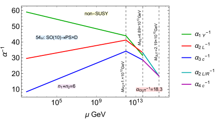
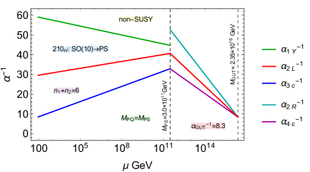
Figure 2: One-loop gauge coupling unification for non-SUSY $SO(10)$ model for two different scenarios: (i) symmetry breaking with $54_{H}$ Higgs (upper plot), (ii) symmetry breaking with $210_{H}$ without $D$-parity (lower plot). In both cases six pairs of vector-like fermions are kept at the PQ scale.

In the second case, we achieve the GUT symmetry breaking via $210_{H}$ Higgs, and assume the absence of $D$-parity Chang:1985zq at the PS scale. In this case we also take the PQ and the PS breaking scale to be the same, $M_{PQ}=M_{PS}$. Moreover, above the intermediate scale gauge beta functions receive contributions from the clockwork sector as before, as well as contributions from $(2,2,15),(1,3,\overline{10})\subset\overline{126}_{H}$, and a complex $(2,2,1)\subset 10_{H}$ of Higgs bosons. The beta function coefficients are $b_{i}=\{18,74/3,41/3\}$ (here $i=1,2,3$ correspond to $SU(2)_{L}$, $SU(2)_{R}$, and $SU(4)_{C}$ respectively).

Perturbative gauge coupling unification can be obtained in each of the aforementioned scenarios, and these results are presented in Fig. 2. We have used one-loop RGE and ignored high scale threshold effects in generating these figures. From Fig. 2, one clearly sees the advantage of employing a $210_{H}$ Higgs. First of all, it is possible in this case to identify the PS scale with the PQ scale. Furthermore, unification occurs at around $2.35\times 10^{16}$ GeV, which implies that proton lifetime arising from gauge boson mediated processes is sufficiently long. The larger unification scale is correlated with the smaller intermediate PS scale, which is realized since the $210_{H}$ breaks $SO(10)$ down to the PS symmetry without $D$ parity. When a $54_{H}$ is used to break $SO(10)$ symmetry instead of the $210_{H}$, one sees that the unification scale is relatively low, about $2\times 10^{15}$ GeV. This is correlated with a larger intermediate PS scale, which is a consequence of an unbroken $D$-parity. It is this symmetry that requires the $SU(2)_{L}$ partner of the $(10,1,3)$ Higgs multiplet to have mass at the PS scale, thus affecting the gauge coupling evolution more drastically. A null observation of proton decay requires the GUT scale to be $M_{GUT}\geq 5\times 10^{15}$ GeV. It has been shown that including high scale threshold corrections this model can indeed be consistent with proton lifetime limits Babu:2015bna . It should also be noted that a $45_{H}$ can be used to break the GUT symmetry, but the viability of this scenario relies on quantum corrections in the Higgs potential Graf:2016znk . We note that the analysis performed in the Yakawa sector remains valid regardless of the choice of the Higgs field that breaks the GUT symmetry.

In the case of non-SUSY $SO(10)$ embedded with clockwork chain, the gauge couplings remain perturbative all the way to the Planck scale. The beta-function coefficient $b$, where $dg/dt=bg^{3}/(16\pi^{2})$, changes from $-34/3$ to $+14/3$ with the addition of six pairs of $16+\bar{16}$ of the clockwork sector as an example. (This choice is not unique, however.) This leaves the gauge coupling perturbative up to the Planck scale. Here we assumed that an additional $54$ Higgs is involved in $SO(10)$ symmetry breaking.

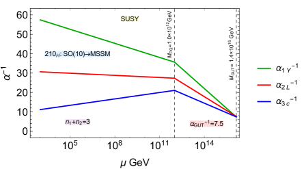
Figure 3: Gauge coupling unification for SUSY $SO(10)$ model with three sets of vector-like $16+\overline{16}$ fermions added at the PQ scale. For this illustration, we set $M_{SUSY}=1$ TeV and used the one-loop RGE evolution of gauge couplings.

3.3 SUSY $SO(10)$ with PQ symmetry

The Peccei-Quinn symmetry can be implemented in the SUSY $SO(10)$ framework along the line discussed in the previous subsection. With the PQ symmetry, the unwanted couplings of the $210_{H}$ field with the vector-like fermions will be forbidden, and there would be no need for a $Z_{4}$ symmetry adopted in Sec. 3.1. This however, modifies the successful gauge coupling unification of the MSSM. The reason is that, in this set-up, the vector-like fermions acquire their masses only after the PQ symmetry is broken. Hence, above the PQ scale, the beta function coefficients for the gauge coupling evolution receive additional contributions. Consequently, perturbative unification of gauge couplings even up to the GUT scale becomes challenging. We have checked that unlike the non-SUSY case, adding six pairs of vector-like fermions at the PQ scale certainly does not work for the SUSY scenario. In Fig. 3, we demonstrate a viable perturbative one-loop gauge coupling unification scenario, with three vector-like fermion pairs $16+\overline{16}$ having masses at the PQ scale. In this analysis, we evolve the MSSM RGEs from the SUSY scale ($M_{SUSY}=$ 1 TeV) up to the PQ scale with the MSSM beta function coefficients $b_{i}=\{33/5,1,-3\}$. The input values at the TeV scale for the gauge couplings are taken to be $\alpha^{-1}_{1}(M_{SUSY})=57.43$, $\alpha^{-1}_{1}(M_{SUSY})=30.67$, and $\alpha^{-1}_{1}(M_{SUSY})=11.19$ Antusch:2013jca . Then at the PQ scale, we add contributions from three pairs of vector-like fermions that modifies the new beta function coefficients to be $b_{i}=\{93/5,13,9\}$ and further run the RGEs up to the GUT scale. Whereas Fig. 3 shows the consistency of keeping three vector-like pairs at the intermediate scale, adding any more pairs would bring the theory to a nonperturbative regime before reaching the GUT scale. Since the implementation of clockwork mechanism typically requires larger number of vector-like states, this scenario with the added PQ symmetry is not a preferred option, since it makes clockwork not very efficient. Furthermore, due to the presence of the plethora of fields lurking around the GUT scale, large threshold corrections are expected to play vital role in the running of the gauge couplings (see for example Ref. Aulakh:2013lxa ), which we have not taken into consideration. However, even this scenario can explain partially the hierarchies in the fermion and mixing angles.

4 Fit to the fermion spectrum

4.1 SUSY case

To fit the fermion masses and mixings, we perform a $\chi^{2}$ analysis, for which we closely follow the procedure discussed in detail in Refs. Babu:2018tfi ; Babu:2018qca . From Eq. (2.15), first we obtain the fermion mass matrices which have the following form:

$$M_{d}=\Lambda^{T}(H+F)\Lambda\;,$$ (4.38)

$$M_{u}=r\Lambda^{T}(H+sF)\Lambda\;,$$ (4.39)

$$M_{e}=\Lambda^{T}(H-3F)\Lambda\;,$$ (4.40)

$$M^{\nu}_{D}=r\Lambda^{T}(H-3sF)\Lambda\;,$$ (4.41)

$$M_{R}=r_{R}\Lambda^{T}F\Lambda\;,$$ (4.42)

$$M_{N}=-{M^{\nu}_{D}}^{T}M_{R}^{-1}M^{\nu}_{D}\;,$$ (4.43)

where we have defined

$$r=\frac{v^{10}_{u}}{v^{10}_{d}},\;\;\;s=\frac{1}{r}\frac{v^{126}_{u}}{v^{126}_{d}},\;\;\;r_{R}=\frac{v_{R}}{v^{126}_{d}},$$ (4.44)

$$H=v^{10}_{d}Y_{10},\;\;\;F=v^{126}_{d}Y_{126}\;.$$ (4.45)

Here $v_{u}^{10}$ is the VEV of the up-type Higgs doublet from $10_{H}$, etc. As in Ref. Babu:2018tfi , these mass matrices are written in $f^{c}M_{f}f$ basis. Note that in Eq. (4.43), the type-II contributions to neutrino mass is omitted, since the weak triplets have masses of order the GUT scale, hence the corresponding type-II contributions are negligible.

In our numerical analysis, we will take these ratios $r$ and $s$ given in Eq. (4.44) to be free parameters. Note however that, in a theory where the Higgs sector is completely specified, these ratios are related to the parameters that appear in the Higgs potential. Since the focus of the present work is on the minimal Yukawa sector, rather than a minimal and complete symmetry breaking sector, we do not make such a connection here. Detailed studies along this line have been made in Refs. Aulakh:2006hs ; Aulakh:2008sn ; Aulakh:2013lxa ; Babu:2018tfi ; Babu:2018qca .

It should be pointed out that due to the presence of the right-handed neutrinos that have masses a few orders less than the GUT scale, the running of the RGEs from the $M_{Z}$ scale to the $M_{GUT}$ get modified. We properly include these corrections to the Yukawa couplings due to the intermediate scale threshold; for details of this implementation we refer the reader to Ref. Babu:2018tfi . Furthermore, we take the GUT scale values of the charged fermion masses and CKM mixing parameters from Ref. Babu:2018qca . In this procedure, the Yukawa couplings, the CKM parameters, and the $d=5$ effective operator for neutrino masses and mixings are run from the $M_{Z}$ scale to the SUSY scale, which is chosen to be 1 TeV. Above this scale, the full MSSM RGEs are used up to the GUT scale. For neutrinos, on the contrary, the $d=5$ effective operator running is carried out up to the intermediate scale. For neutrinos, we have taken the low energy values from the recent global fit performed in Ref. deSalas:2020pgw . These input values are collected in the second column in Table. IV.

We remind the reader that the original Yukawa couplings $Y_{10}$ and $Y_{126}$ are allowed to have entries that are $\sim\mathcal{O}(1)$, whereas the hierarchies among different generations are generated via the suppression factors ${\color[rgb]{1,0,0}\epsilon_{1}}$ and ${\color[rgb]{0,0,1}\epsilon_{2}}$ originating from the clockwork sector. It is crucial to understand that compared to the minimal $SO(10)$ Yukawa sector, our setup does not introduce any new parameters into the theory. In our fit, we fix $\tan\beta=v_{u}/v_{d}=10$, where $v_{u}$ and $v_{d}$ are the VEVs of the MSSM fields $H^{MSSM}_{u}$ and $H^{MSSM}_{d}$. With these, we find an excellent fit that corresponds to $\chi^{2}=7.98$; the best fit values and the associated pulls are presented in the third and the fourth columns of Table. IV. The full set of best fit parameter values can be found in Appendix B.1. From this fit, we chose the following suppression factors

$$\Lambda=\begin{pmatrix}{\color[rgb]{1,0,0}\epsilon_{1}}&0&0\\ 0&{\color[rgb]{0,0,1}\epsilon_{2}}&0\\ 0&0&1\end{pmatrix}=\begin{pmatrix}0.06117&0&0\\ 0&0.32983&0\\ 0&0&1\end{pmatrix}.$$ (4.46)

Here ${\color[rgb]{1,0,0}\epsilon_{1}}\simeq\lambda^{2}$ and ${\color[rgb]{0,0,1}\epsilon_{2}}\simeq\lambda$, with $\lambda=\sin\theta_{c}$, where $\theta_{c}$ is the Cabibbo angle. A choice of these values for ${\color[rgb]{1,0,0}\epsilon_{1}}$ and ${\color[rgb]{0,0,1}\epsilon_{2}}$ correspond to $q_{1}=1.93445,\;q_{2}=1.55098$ for $n_{1}=4,\;n_{2}=2$. The down-quark and up-quark mass matrices (after taking into account the intermediate scale threshold corrections) corresponding to the best fit are then given below, which explicitly demonstrates how clockwork is responsible for generating the required hierarchies in the fermion masses and mixings. All other mass matrices can be readily obtained from these two matrices (or from the parameter set given in Appendix B.1).

$$M_{d}=0.80166e^{2.18422i}\begin{pmatrix}1.27815\;{\color[rgb]{1,0,0}\epsilon_{1}^{2}}\;e^{-3.0004i}&1.26174\;{\color[rgb]{1,0,0}\epsilon_{1}}{\color[rgb]{0,0,1}\epsilon_{2}}\;e^{-2.71759i}&1.11777\;{\color[rgb]{1,0,0}\epsilon_{1}}\;e^{1.63891i}\\ 1.26174\;{\color[rgb]{1,0,0}\epsilon_{1}}{\color[rgb]{0,0,1}\epsilon_{2}}\;e^{-2.71759i}&1.61178\;{\color[rgb]{0,0,1}\epsilon_{2}^{2}}\;e^{-2.31606i}&1.20224\;{\color[rgb]{0,0,1}\epsilon_{2}}\;e^{2.02843i}\\ 1.11777\;{\color[rgb]{1,0,0}\epsilon_{1}}\;e^{1.63891i}&1.20224\;{\color[rgb]{0,0,1}\epsilon_{2}}\;e^{2.02843i}&1\end{pmatrix}\;\text{GeV},$$ (4.47)

$$M_{u}=79.1467e^{2.27241i}\begin{pmatrix}1.09514\;{\color[rgb]{1,0,0}\epsilon_{1}^{2}}\;e^{3.10025i}&1.17556\;{\color[rgb]{1,0,0}\epsilon_{1}}{\color[rgb]{0,0,1}\epsilon_{2}}\;e^{-2.80578i}&1.04143\;{\color[rgb]{1,0,0}\epsilon_{1}}\;e^{1.55072i}\\ 1.17556\;{\color[rgb]{1,0,0}\epsilon_{1}}{\color[rgb]{0,0,1}\epsilon_{2}}\;e^{-2.80578i}&1.24674\;{\color[rgb]{0,0,1}\epsilon_{2}^{2}}\;e^{-2.42765i}&1.12012\;{\color[rgb]{0,0,1}\epsilon_{2}}\;e^{1.94025i}\\ 1.04143\;{\color[rgb]{1,0,0}\epsilon_{1}}\;e^{1.55072i}&1.12012\;{\color[rgb]{0,0,1}\epsilon_{2}}\;e^{1.94025i}&1\end{pmatrix}\;\text{GeV}.$$ (4.48)

It can be seen from the above matrices that all the Yukawa couplings are very close to 1. Even thought in writing Eqs. (4.47) and (4.48) we have used the clockwork chain lengths to be $n_{1}=4$ and $n_{2}=2$, however, from the best fit parameters presented in Appendix B.1 various different chain lengths can be considered without needing to modify the fit at all. By demanding order unity Yukawa couplings, this corresponds to longer chain length for $q_{i}$ very close to 1, and shorter chain length when $q_{i}$ starts to become larger than 1. Finally, the analysis presented here can be trivially extended for the case $\beta_{1}\neq 1$ discussed in Sec. 2.2. In the case of SUSY $SO(10)$ with a Peccei-Quinn symmetry, concentrating on the gauge coupling unification scenario presented in Fig. 3, where we have assumed $n_{1}+n_{2}=3$, setting $n_{1}=2$ and $n_{2}=1$ returns $q_{1}=3.9779$ and $q_{2}=2.8622$, which are not too far from unity.

Note that the parameters of this class of models cannot be chosen randomly. There is a GUT sum rule involving the masses and mixings in the model. This should not be considered as a fine-tuning of parameters, rather it is a result of a GUT symmetry. This has been noted in the Ref. Babu:1992ia , and the sum rule has been explicitly worked out in Ref. Lavoura:1993vz for the case of real parameters. Indeed, in the case of all parameters being real, one can write $M_{\ell}=aM_{u}+bM_{d}$, with the mass matrices being symmetric. In a basis where $M_{u}$ is diagonal, $M_{d}=V.M_{d}^{\rm diagonal}.V^{T}$, where $V$ is the CKM matrix. Thus all elements of the charged lepton mass matrix $M_{\ell}$ is determined in terms of the quark masses, CKM mixing angles and the two free parameters $(a,\,b)$. This leads to one sum rule involving the masses of the charged fermions. Even with the inclusion of phases the GUT mass sum rule is present in the model, the corresponding relation becomes more involved. However, for any given set of masses and mixings the magnitudes as well as the phases are constrained, such that this mass sum rule is satisfied. This constraint is implemented numerically in our fits, and as a result, the order one complex parameters in Eqs. (4.47) and (4.48) cannot be arbitrarily chosen (the same argument goes for the fit associated to Eqs. (4.50) and (4.51)). This mass sum rule is a prediction of $SO(10)$ GUT, which prevails in our clockwork extension.

Before closing this section we compare the fit we obtain here with the fit presented in Ref. Babu:2018qca . In the present work the total $\chi^{2}$ obtained is about 8, whereas, it is about 6 in Ref. Babu:2018qca . The reason for obtaining a slightly higher $\chi^{2}$ is mainly due to the fact that in this work in the fitting procedure, we have included the Dirac phase in the lepton sector as well, which was left out in the $\chi^{2}$-minimization in Ref. Babu:2018qca . Additionally, in the prsent work, we have taken the recent global fit values of the neutrinos, which have somewhat smaller experimental uncertainties compared to the previously used values in Ref. Babu:2018qca .

Observables	SUSY			non-SUSY
(masses in GeV)	Input	Best Fit	Pull	Input	Best Fit	Pull
$m_{u}/10^{-3}$	0.502$\pm$0.155	0.515	0.08	0.442$\pm$0.149	0.462	0.13
$m_{c}$	$0.245\pm$0.007	0.246	0.14	0.238$\pm$0.007	0.239	0.18
$m_{t}$	90.28$\pm$0.89	90.26	-0.02	74.51$\pm$0.65	74.47	-0.05
$m_{b}/10^{-3}$	0.839$\pm$0.17	0.400	-2.61	1.14$\pm$0.22	0.542	-2.62
$m_{s}/10^{-3}$	$16.62\pm$0.90	16.53	-0.09	21.58$\pm$1.14	22.57	0.86
$m_{b}$	$0.938\pm$0.009	0.933	-0.55	0.994$\pm$0.009	0.995	0.19
$m_{e}/10^{-3}$	0.3440$\pm$0.0034	0.344	0.08	0.4707$\pm$0.0047	0.470	-0.03
$m_{\mu}/10^{-3}$	72.625$\pm$0.726	72.58	-0.05	99.365$\pm$0.993	99.12	-0.24
$m_{\tau}$	1.2403$\pm$0.0124	1.247	0.57	1.6892$\pm$0.0168	1.688	-0.05
$|V_{us}|/10^{-2}$	$22.54\pm$0.07	22.54	0.02	22.54$\pm$0.06	22.54	0.06
$|V_{cb}|/10^{-2}$	3.93$\pm$0.06	3.908	-0.42	4.856$\pm$0.06	4.863	0.13
$|V_{ub}|/10^{-2}$	0.341$\pm$0.012	0.341	0.003	0.420$\pm$0.013	0.421	0.10
$\delta_{CKM}^{\circ}$	69.21$\pm$3.09	69.32	0.03	69.15$\pm$3.09	70.24	0.35
$\Delta m^{2}_{21}/10^{-5}(eV^{2})$	8.982$\pm$0.25	8.972	-0.04	12.65$\pm$0.35	12.65	-0.01
$\Delta m^{2}_{31}/10^{-3}(eV^{2})$	3.05$\pm$0.04	3.056	0.02	4.307$\pm$0.059	4.307	0.006
$\sin^{2}\theta_{12}$	0.318$\pm$0.016	0.314	-0.19	0.318$\pm$0.016	0.316	-0.07
$\sin^{2}\theta_{23}$	0.563$\pm$0.019	0.563	0.031	0.563$\pm$0.019	0.563	0.01
$\sin^{2}\theta_{13}$	0.0221$\pm$0.0006	0.0221	-0.003	0.0221$\pm$0.0006	0.0220	-0.16
$\delta_{CP}^{\circ}$	224.1$\pm$33.3	240.1	0.48	224.1$\pm$33.3	225.1	0.03
$\chi^{2}$	-	-	7.98	-	-	7.96

Table IV: Inputs and the corresponding best fit values of the observables along with their pulls at the GUT scale $\mu=2\times 10^{16}$ GeV for both SUSY and non-SUSY cases are summarized here. In both these cases, type-I seesaw dominance is assumed, for details see text.

4.2 Non-SUSY case

To get the GUT scale values of the fermion masses and mixings for the non-SUSY scenario, we closely follow the procedure discussed in Ref. Babu:2016bmy . In this method, the low scale values are evolved up to the GUT scale using SM RGEs. However, this one-step RGE running receives corrections due to the intermediate scale right-handed neutrinos. In our numerical fit, we take into account these modification of the Yukawa couplings following the method detailed in Ref. Babu:2016bmy , where a basis of $fM_{ij}f^{c}$ is used, and we stay with such a basis. Then, for the non-SUSY case, the mass matrices Eqs. (4.38) - (4.43) derived in the previous section are still applicable with the only exception that $M_{\nu}^{D}$ should be transposed in Eq. (4.43). As before, we focus on the type-I dominance scenario for the neutrino masses. It is to be pointed out that type-II seesaw for non-SUSY case fails to provide a realistic fit Joshipura:2011nn . The GUT scale inputs for charged fermion masses and mixings are obtained from Ref. Babu:2016bmy , whereas for neutrinos, we have collected the recent low scale values from Ref. deSalas:2020pgw , and evolved the $d=5$ effective operator up to the right-handed neutrino mass scale. These input parameters are summarized in the fifth column of Table. IV. A good fit to these data is obtained from our numerical procedure, and the the best fit corresponds to $\chi^{2}=7.96$. The best fit values for physical quantities and their pulls are presented in the sixth and the seventh columns of Table. IV. The theory parameters of this best fit are summarized in Appendix B.2. As before, no new parameters enter in this fit process compared to the minimal $SO(10)$ Yukawa sector. Hence, our fit is applicable for cases with or without clockwork extension (for both SUSY and non-SUSY models). Following our previous analysis, we fix the clockwork chain lengths to be $n_{1}=4,\;n_{2}=2$, then the corresponding chosen suppression factors are

$$\Lambda=\begin{pmatrix}{\color[rgb]{1,0,0}\epsilon_{1}}&0&0\\ 0&{\color[rgb]{0,0,1}\epsilon_{2}}&0\\ 0&0&1\end{pmatrix}=\begin{pmatrix}0.03783&0&0\\ 0&0.23973&0\\ 0&0&1\end{pmatrix}.$$ (4.49)

Like in the SUSY case, here we also get suppression factors of same order: ${\color[rgb]{1,0,0}\epsilon_{1}}\simeq\lambda^{2}$ and ${\color[rgb]{0,0,1}\epsilon_{2}}\simeq\lambda$ that amount to $q_{1}=2.20312,\;q_{2}=1.89219$. The associated down-quark and up-quark mass matrices (after taking into account the intermediate scale threshold corrections) are found to be

$$M_{d}=0.94968e^{-1.68947i}\begin{pmatrix}1.45089\;{\color[rgb]{1,0,0}\epsilon_{1}^{2}}\;e^{2.18915i}&0.97791\;{\color[rgb]{1,0,0}\epsilon_{1}}{\color[rgb]{0,0,1}\epsilon_{2}}\;e^{2.37807i}&1.10034\;{\color[rgb]{1,0,0}\epsilon_{1}}\;e^{1.04364i}\\ 0.97791\;{\color[rgb]{1,0,0}\epsilon_{1}}{\color[rgb]{0,0,1}\epsilon_{2}}\;e^{2.37807i}&1.22764\;{\color[rgb]{0,0,1}\epsilon_{2}^{2}}\;e^{2.18995i}&0.89334\;{\color[rgb]{0,0,1}\epsilon_{2}}\;e^{1.09213i}\\ 1.10034\;{\color[rgb]{1,0,0}\epsilon_{1}}\;e^{1.04364i}&0.89334\;{\color[rgb]{0,0,1}\epsilon_{2}}\;e^{1.09213i}&1\end{pmatrix}\;\text{GeV},$$ (4.50)

$$M_{u}=71.505e^{1.23138i}\begin{pmatrix}1.11401\;{\color[rgb]{1,0,0}\epsilon_{1}^{2}}\;e^{2.51117i}&0.91309\;{\color[rgb]{1,0,0}\epsilon_{1}}{\color[rgb]{0,0,1}\epsilon_{2}}\;e^{2.5988i}&1.0274\;{\color[rgb]{1,0,0}\epsilon_{1}}\;e^{1.26437i}\\ 0.91309\;{\color[rgb]{1,0,0}\epsilon_{1}}{\color[rgb]{0,0,1}\epsilon_{2}}\;e^{2.5988i}&0.73257\;{\color[rgb]{0,0,1}\epsilon_{2}^{2}}\;e^{2.69088i}&0.83413\;{\color[rgb]{0,0,1}\epsilon_{2}}\;e^{1.31287i}\\ 1.0274\;{\color[rgb]{1,0,0}\epsilon_{1}}\;e^{1.26437i}&0.83413\;{\color[rgb]{0,0,1}\epsilon_{2}}\;e^{1.31287i}&1\end{pmatrix}\;\text{GeV}.$$ (4.51)

All the conclusion we have reached for the SUSY case are also applicable in this non-SUSY scenario.

From the results presented in the previous subsection as well as in this subsection, it is clear that our simple clockwork extension to the minimal Yukawa sector of $SO(10)$ with or without SUSY naturally explains the hierarchies in the fermion spectrum.

5 Conclusion

In this work, we have presented a minimal and highly predictive mechanism to address the flavor puzzle. In particular, our proposed framework is based on the minimal Yukawa sector of $SO(10)$ GUT with or without SUSY, extended with two clockwork chains. Each of these chains consists of a set of $16+\overline{16}$ vector-like fermions that couples indistinguishably with different fermion generations. Whereas $SO(10)$ symmetry correlates different fermion sectors, clockwork sector supplies proper suppression factors to incorporate the required hierarchies. The proposed setup to explain the origin of flavor hierarchies is simple in its construction and is also renormalizable. All Yukawa couplings of these theories are of order unity which is shown to provide a consistent fit to the fermion masses and mixings. Detailed numerical analysis has been carried out, and the results summarized in Table IV to demonstrate the robustness of the theory.

Appendix

Appendix A Expressions for $\lambda_{i}$ and $K_{1,2}$

In this Appendix we present the exact analytical forms for $\lambda_{i}$ and $K_{1,2}$ matrices as defined in Eq. (2.28):

$$\begin{pmatrix}\frac{q_{1}^{2}-q_{1}^{-2n_{1}}}{q_{1}^{2}-1}&0&0\\ -\frac{q_{3}}{q_{2}}q_{1}^{-2n_{1}}&\frac{{q_{2}}^{2}-{q_{2}}^{-2n_{2}}}{{q_{2}}^{2}-1}&0\\ 0&0&1\end{pmatrix}\equiv\begin{pmatrix}a&0&0\\ b&c&0\\ 0&0&1\end{pmatrix}=K_{1}\begin{pmatrix}\lambda_{1}&0&0\\ 0&\lambda_{2}&0\\ 0&0&1\end{pmatrix}K^{T}_{2}.$$ (A.52)

$$\lambda_{1,2}=\left[\frac{1}{2}\left(a^{2}+b^{2}+c^{2}\mp\sqrt{a^{2}+b^{2}+c^{2}-4a^{2}c^{2}}\right)\right]^{1/2}.$$ (A.53)

$$K_{1}=\left(\begin{array}[]{ccc}-\frac{-a^{2}+b^{2}+c^{2}+\sqrt{a^{4}+2\left(b^{2}-c^{2}\right)a^{2}+\left(b^{2}+c^{2}\right)^{2}}}{2ab\sqrt{\frac{\left(-a^{2}+b^{2}+c^{2}+\sqrt{a^{4}+2\left(b^{2}-c^{2}\right)a^{2}+\left(b^{2}+c^{2}\right)^{2}}\right)^{2}}{4a^{2}b^{2}}+1}}&-\frac{-a^{2}+b^{2}+c^{2}-\sqrt{a^{4}+2\left(b^{2}-c^{2}\right)a^{2}+\left(b^{2}+c^{2}\right)^{2}}}{2ab\sqrt{\frac{\left(a^{2}-b^{2}-c^{2}+\sqrt{a^{4}+2\left(b^{2}-c^{2}\right)a^{2}+\left(b^{2}+c^{2}\right)^{2}}\right)^{2}}{4a^{2}b^{2}}+1}}&0\\ \frac{1}{\sqrt{\frac{\left(-a^{2}+b^{2}+c^{2}+\sqrt{a^{4}+2\left(b^{2}-c^{2}\right)a^{2}+\left(b^{2}+c^{2}\right)^{2}}\right)^{2}}{4a^{2}b^{2}}+1}}&\frac{1}{\sqrt{\frac{\left(a^{2}-b^{2}-c^{2}+\sqrt{a^{4}+2\left(b^{2}-c^{2}\right)a^{2}+\left(b^{2}+c^{2}\right)^{2}}\right)^{2}}{4a^{2}b^{2}}+1}}&0\\ 0&0&1\end{array}\right).$$ (A.57)

$$K_{2}=\left(\begin{array}[]{ccc}-\frac{-a^{2}-b^{2}+c^{2}+\sqrt{a^{4}+2\left(b^{2}-c^{2}\right)a^{2}+\left(b^{2}+c^{2}\right)^{2}}}{2bc\sqrt{\frac{\left(a^{2}+b^{2}-c^{2}-\sqrt{a^{4}+2\left(b^{2}-c^{2}\right)a^{2}+\left(b^{2}+c^{2}\right)^{2}}\right)^{2}}{4b^{2}c^{2}}+1}}&\frac{1}{\sqrt{\frac{\left(a^{2}+b^{2}-c^{2}-\sqrt{a^{4}+2\left(b^{2}-c^{2}\right)a^{2}+\left(b^{2}+c^{2}\right)^{2}}\right)^{2}}{4b^{2}c^{2}}+1}}&0\\ -\frac{-a^{2}-b^{2}+c^{2}-\sqrt{a^{4}+2\left(b^{2}-c^{2}\right)a^{2}+\left(b^{2}+c^{2}\right)^{2}}}{2bc\sqrt{\frac{\left(a^{2}+b^{2}-c^{2}+\sqrt{a^{4}+2\left(b^{2}-c^{2}\right)a^{2}+\left(b^{2}+c^{2}\right)^{2}}\right)^{2}}{4b^{2}c^{2}}+1}}&\frac{1}{\sqrt{\frac{\left(a^{2}+b^{2}-c^{2}+\sqrt{a^{4}+2\left(b^{2}-c^{2}\right)a^{2}+\left(b^{2}+c^{2}\right)^{2}}\right)^{2}}{4b^{2}c^{2}}+1}}&0\\ 0&0&1\end{array}\right).$$ (A.61)

Appendix B Best fit parameters

As discussed in the main text, the Yukawa sector is effectively identical to the minimal $SO(10)$ model. It is because the clockwork sector does not introduce any new parameters, rather it accounts for the hierarchical factors. Hence, the fit we perform is identical to the minimal Yukawa sector of $SO(10)$ model. Also our fit can be used for arbitrary lengths of the clockwork chains. Due to these attractive features, in the following, for the convenience of the readers, we present our best fit parameters in the form that is readily used for general purpose. Following Refs. Babu:2016bmy ; Babu:2018tfi we present the best fit parameters in a basis where the $\Lambda^{T}Y_{126}\Lambda$ is diagonal and real. We have used these best fit parameters to reconstruct the down-quark and up-quark mass matrices, which are presented in Eqs. (4.47) - (4.48) and in Eqs. (4.50) - (4.51) for SUSY and non-SUSY models, respectively. As can be seen from these mass matrices, all the Yukawa couplings are of the same order and in fact very close to unity, which is our desired result. Note however that besides the Yukawa couplings, a fit to the fermion spectrum contains two VEV ratios $s$ and $r$ as defined in Eq. (4.44). For the former, our fit prefers a value of $s\simeq\lambda$, and for the latter $r\simeq m_{t}/m_{b}$ is required. These VEV ratios do not have any direct connection to the Yukawa couplings and do not necessarily have to be of order unity. Within our framework, their values are predicted directly from a fit to the data.

B.1 SUSY $SO(10)$

$$r=93.9719,\;s=2.96269\times 10^{-1}+1.27201\times 10^{-2}i,\;r_{R}=8.73689\times 10^{12}\;,$$ (B.62)

$$\Lambda^{T}F\Lambda=10^{-1}\left(\begin{array}[]{ccc}6.59098\times 10^{-3}&0.&0.\\ 0.&3.41720\times 10^{-1}&0.\\ 0.&0.&1.33390\\ \end{array}\right)\;\text{GeV},$$ (B.66)

$$\Lambda^{T}H\Lambda=10^{-3}\left(\begin{array}[]{ccc}1.96740\,-2.79338i&17.5736\,-10.3763i&-42.5697-34.5327i\\ 17.5736\,-10.3763i&105.17\,-18.4787i&-152.329-279.013i\\ -42.5697-34.5327i&-152.329-279.013i&-594.884+655.504i\\ \end{array}\right)\;\text{GeV}.$$ (B.70)

B.2 Non-SUSY $SO(10)$

$$r=70.3027,\;s=2.57526\times 10^{-1}+5.27538\times 10^{-2}i,\;r_{R}=4.57993\times 10^{12}\;,$$ (B.71)

$$\Lambda^{T}F\Lambda=10^{-1}\left(\begin{array}[]{ccc}5.29819\times 10^{-3}&0&0\\ 0&3.82033\times 10^{-1}&0\\ 0&0&3.04637\\ \end{array}\right)\;\text{GeV},$$ (B.75)

$$\Lambda^{T}H\Lambda=10^{-3}\left(\begin{array}[]{ccc}1.20097\,-0.94480i&6.50337\,-5.35207i&31.5693\,+23.7924i\\ 6.50337\,-5.35207i&20.5847\,-32.1521i&168.169\,+114.396i\\ 31.5693\,+23.7924i&168.169\,+114.396i&-417.079+943.005i\\ \end{array}\right)\;\text{GeV}.$$ (B.79)

References

- (1) J. C. Pati and A. Salam, “Lepton Number as the Fourth Color,” Phys. Rev. D 10 (1974) 275–289. [Erratum: Phys.Rev.D 11, 703–703 (1975)].
- (2) H. Georgi and S. Glashow, “Unity of All Elementary Particle Forces,” Phys. Rev. Lett. 32 (1974) 438–441.
- (3) H. Georgi, H. R. Quinn, and S. Weinberg, “Hierarchy of Interactions in Unified Gauge Theories,” Phys. Rev. Lett. 33 (1974) 451–454.
- (4) H. Georgi, “The State of the Art—Gauge Theories,” AIP Conf. Proc. 23 (1975) 575–582.
- (5) H. Fritzsch and P. Minkowski, “Unified Interactions of Leptons and Hadrons,” Annals Phys. 93 (1975) 193–266.
- (6) P. Minkowski, “ at a Rate of One Out of Muon Decays?,” Phys. Lett. B 67 (1977) 421–428.
- (7) T. Yanagida, “Horizontal gauge symmetry and masses of neutrinos,” Conf. Proc. C 7902131 (1979) 95–99.
- (8) S. Glashow, “The Future of Elementary Particle Physics,” NATO Sci. Ser. B 61 (1980) 687.
- (9) M. Gell-Mann, P. Ramond, and R. Slansky, “Complex Spinors and Unified Theories,” Conf. Proc. C 790927 (1979) 315–321, arXiv:1306.4669 [hep-th].
- (10) R. N. Mohapatra and G. Senjanovic, “Neutrino Mass and Spontaneous Parity Nonconservation,” Phys. Rev. Lett. 44 (1980) 912.
- (11) R. Peccei and H. R. Quinn, “CP Conservation in the Presence of Instantons,” Phys. Rev. Lett. 38 (1977) 1440–1443.
- (12) K. Babu and R. Mohapatra, “Predictive neutrino spectrum in minimal SO(10) grand unification,” Phys. Rev. Lett. 70 (1993) 2845–2848, arXiv:hep-ph/9209215.
- (13) B. Bajc, G. Senjanovic, and F. Vissani, “How neutrino and charged fermion masses are connected within minimal supersymmetric SO(10),” PoS HEP2001 (2001) 198, arXiv:hep-ph/0110310 [hep-ph].
- (14) B. Bajc, G. Senjanovic, and F. Vissani, “b - tau unification and large atmospheric mixing: A Case for noncanonical seesaw,” Phys. Rev. Lett. 90 (2003) 051802, arXiv:hep-ph/0210207 [hep-ph].
- (15) T. Fukuyama and N. Okada, “Neutrino oscillation data versus minimal supersymmetric SO(10) model,” JHEP 11 (2002) 011, arXiv:hep-ph/0205066 [hep-ph].
- (16) H. S. Goh, R. N. Mohapatra, and S.-P. Ng, “Minimal SUSY SO(10), b tau unification and large neutrino mixings,” Phys. Lett. B570 (2003) 215–221, arXiv:hep-ph/0303055 [hep-ph].
- (17) H. S. Goh, R. N. Mohapatra, and S.-P. Ng, “Minimal SUSY SO(10) model and predictions for neutrino mixings and leptonic CP violation,” Phys. Rev. D68 (2003) 115008, arXiv:hep-ph/0308197 [hep-ph].
- (18) S. Bertolini, M. Frigerio, and M. Malinsky, “Fermion masses in SUSY SO(10) with type II seesaw: A Non-minimal predictive scenario,” Phys. Rev. D70 (2004) 095002, arXiv:hep-ph/0406117 [hep-ph].
- (19) S. Bertolini and M. Malinsky, “On CP violation in minimal renormalizable SUSY SO(10) and beyond,” Phys. Rev. D 72 (2005) 055021, arXiv:hep-ph/0504241.
- (20) K. S. Babu and C. Macesanu, “Neutrino masses and mixings in a minimal SO(10) model,” Phys. Rev. D72 (2005) 115003, arXiv:hep-ph/0505200 [hep-ph].
- (21) S. Bertolini, T. Schwetz, and M. Malinsky, “Fermion masses and mixings in SO(10) models and the neutrino challenge to SUSY GUTs,” Phys. Rev. D73 (2006) 115012, arXiv:hep-ph/0605006 [hep-ph].
- (22) B. Bajc, I. Dorsner, and M. Nemevsek, “Minimal SO(10) splits supersymmetry,” JHEP 11 (2008) 007, arXiv:0809.1069 [hep-ph].
- (23) A. S. Joshipura and K. M. Patel, “Fermion Masses in SO(10) Models,” Phys. Rev. D83 (2011) 095002, arXiv:1102.5148 [hep-ph].
- (24) G. Altarelli and D. Meloni, “A non supersymmetric SO(10) grand unified model for all the physics below ,” JHEP 08 (2013) 021, arXiv:1305.1001 [hep-ph].
- (25) A. Dueck and W. Rodejohann, “Fits to SO(10) Grand Unified Models,” JHEP 09 (2013) 024, arXiv:1306.4468 [hep-ph].
- (26) T. Fukuyama, K. Ichikawa, and Y. Mimura, “Revisiting fermion mass and mixing fits in the minimal SUSY GUT,” Phys. Rev. D94 no. 7, (2016) 075018, arXiv:1508.07078 [hep-ph].
- (27) K. S. Babu, B. Bajc, and S. Saad, “Resurrecting Minimal Yukawa Sector of SUSY SO(10),” JHEP 10 (2018) 135, arXiv:1805.10631 [hep-ph].
- (28) K. Babu, T. Fukuyama, S. Khan, and S. Saad, “Peccei-Quinn Symmetry and Nucleon Decay in Renormalizable SUSY (10),” JHEP 06 (2019) 045, arXiv:1812.11695 [hep-ph].
- (29) T. Ohlsson and M. Pernow, “Fits to Non-Supersymmetric SO(10) Models with Type I and II Seesaw Mechanisms Using Renormalization Group Evolution,” JHEP 06 (2019) 085, arXiv:1903.08241 [hep-ph].
- (30) B. Dutta, Y. Mimura, and R. N. Mohapatra, “Neutrino masses and mixings in a predictive SO(10) model with CKM CP violation,” Phys. Lett. B603 (2004) 35–45, arXiv:hep-ph/0406262 [hep-ph].
- (31) B. Dutta, Y. Mimura, and R. N. Mohapatra, “Neutrino mixing predictions of a minimal SO(10) model with suppressed proton decay,” Phys. Rev. D72 (2005) 075009, arXiv:hep-ph/0507319 [hep-ph].
- (32) L. Lavoura, H. Kuhbock, and W. Grimus, “Charged-fermion masses in SO(10): Analysis with scalars in 10+120,” Nucl. Phys. B754 (2006) 1–16, arXiv:hep-ph/0603259 [hep-ph].
- (33) P. M. Ferreira, W. Grimus, D. Jurčiukonis, and L. Lavoura, “Flavour symmetries in a renormalizable SO(10) model,” Nucl. Phys. B906 (2016) 289–320, arXiv:1510.02641 [hep-ph].
- (34) T. Fukuyama, K. Ichikawa, and Y. Mimura, “Relation between proton decay and PMNS phase in the minimal SUSY GUT,” Phys. Lett. B764 (2017) 114–120, arXiv:1609.08640 [hep-ph].
- (35) K. Babu, B. Bajc, and S. Saad, “Yukawa Sector of Minimal SO(10) Unification,” JHEP 02 (2017) 136, arXiv:1612.04329 [hep-ph].
- (36) T. Deppisch, S. Schacht, and M. Spinrath, “Confronting SUSY SO(10) with updated Lattice and Neutrino Data,” JHEP 01 (2019) 005, arXiv:1811.02895 [hep-ph].
- (37) K. Babu, “TASI Lectures on Flavor Physics,” in Theoretical Advanced Study Institute in Elementary Particle Physics: The Dawn of the LHC Era, pp. 49–123. 2010. arXiv:0910.2948 [hep-ph].
- (38) F. Feruglio, “Pieces of the Flavour Puzzle,” Eur. Phys. J. C 75 no. 8, (2015) 373, arXiv:1503.04071 [hep-ph].
- (39) Z.-z. Xing, “Flavor structures of charged fermions and massive neutrinos,” Phys. Rept. 854 (2020) 1–147, arXiv:1909.09610 [hep-ph].
- (40) C. Froggatt and H. B. Nielsen, “Hierarchy of Quark Masses, Cabibbo Angles and CP Violation,” Nucl. Phys. B 147 (1979) 277–298.
- (41) K. Choi and S. H. Im, “Realizing the relaxion from multiple axions and its UV completion with high scale supersymmetry,” JHEP 01 (2016) 149, arXiv:1511.00132 [hep-ph].
- (42) D. E. Kaplan and R. Rattazzi, “Large field excursions and approximate discrete symmetries from a clockwork axion,” Phys. Rev. D 93 no. 8, (2016) 085007, arXiv:1511.01827 [hep-ph].
- (43) G. F. Giudice and M. McCullough, “A Clockwork Theory,” JHEP 02 (2017) 036, arXiv:1610.07962 [hep-ph].
- (44) G. von Gersdorff, “Natural Fermion Hierarchies from Random Yukawa Couplings,” JHEP 09 (2017) 094, arXiv:1705.05430 [hep-ph].
- (45) K. M. Patel, “Clockwork mechanism for flavor hierarchies,” Phys. Rev. D 96 no. 11, (2017) 115013, arXiv:1711.05393 [hep-ph].
- (46) R. Alonso, A. Carmona, B. M. Dillon, J. F. Kamenik, J. Martin Camalich, and J. Zupan, “A clockwork solution to the flavor puzzle,” JHEP 10 (2018) 099, arXiv:1807.09792 [hep-ph].
- (47) F. Sannino, J. Smirnov, and Z.-W. Wang, “Asymptotically safe clockwork mechanism,” Phys. Rev. D 100 no. 7, (2019) 075009, arXiv:1902.05958 [hep-ph].
- (48) A. Smolkovič, M. Tammaro, and J. Zupan, “Anomaly free Froggatt-Nielsen models of flavor,” JHEP 10 (2019) 188, arXiv:1907.10063 [hep-ph].
- (49) F. Abreu de Souza and G. von Gersdorff, “A Random Clockwork of Flavor,” JHEP 02 (2020) 186, arXiv:1911.08476 [hep-ph].
- (50) G. von Gersdorff, “Realistic GUT Yukawa Couplings from a Random Clockwork Model,” arXiv:2005.14207 [hep-ph].
- (51) A. Ibarra, A. Kushwaha, and S. K. Vempati, “Clockwork for Neutrino Masses and Lepton Flavor Violation,” Phys. Lett. B 780 (2018) 86–92, arXiv:1711.02070 [hep-ph].
- (52) A. Banerjee, S. Ghosh, and T. S. Ray, “Clockworked VEVs and Neutrino Mass,” JHEP 11 (2018) 075, arXiv:1808.04010 [hep-ph].
- (53) S. Hong, G. Kurup, and M. Perelstein, “Clockwork Neutrinos,” JHEP 10 (2019) 073, arXiv:1903.06191 [hep-ph].
- (54) T. Kitabayashi, “Clockwork origin of neutrino mixings,” Phys. Rev. D 100 no. 3, (2019) 035019, arXiv:1904.12516 [hep-ph].
- (55) T. Kitabayashi, “Scalar clockwork and flavor neutrino mass matrix,” arXiv:2003.06550 [hep-ph].
- (56) C. Aulakh and R. N. Mohapatra, “Implications of Supersymmetric SO(10) Grand Unification,” Phys. Rev. D 28 (1983) 217.
- (57) T. Clark, T.-K. Kuo, and N. Nakagawa, “A SO(10) SUPERSYMMETRIC GRAND UNIFIED THEORY,” Phys. Lett. B 115 (1982) 26–28.
- (58) C. S. Aulakh, B. Bajc, A. Melfo, G. Senjanovic, and F. Vissani, “The Minimal supersymmetric grand unified theory,” Phys. Lett. B 588 (2004) 196–202, arXiv:hep-ph/0306242.
- (59) B. Bajc, A. Melfo, G. Senjanovic, and F. Vissani, “The Minimal supersymmetric grand unified theory. 1. Symmetry breaking and the particle spectrum,” Phys. Rev. D70 (2004) 035007, arXiv:hep-ph/0402122 [hep-ph].
- (60) K. Babu and S. M. Barr, “Large neutrino mixing angles in unified theories,” Phys. Lett. B 381 (1996) 202–208, arXiv:hep-ph/9511446.
- (61) K. Babu and S. M. Barr, “An SO(10) solution to the puzzle of quark and lepton masses,” Phys. Rev. Lett. 75 (1995) 2088–2091, arXiv:hep-ph/9503215.
- (62) K. S. Babu and S. M. Barr, “Realistic quark and lepton masses through SO(10) symmetry,” Phys. Rev. D56 (1997) 2614–2631, arXiv:hep-ph/9512389 [hep-ph].
- (63) K. Babu, B. Bajc, and S. Saad, “New Class of SO(10) Models for Flavor,” Phys. Rev. D 94 no. 1, (2016) 015030, arXiv:1605.05116 [hep-ph].
- (64) K. Babu, A. Khanov, and S. Saad, “Anarchy with Hierarchy: A Probabilistic Appraisal,” Phys. Rev. D 95 no. 5, (2017) 055014, arXiv:1612.07787 [hep-ph].
- (65) G. D. Smith, Numerical Solution Of Partial Differential Equations. Clarendon Press, Oxford, 1978.
- (66) C. S. Aulakh, “MSGUTs from germ to bloom: Towards falsifiability and beyond,” in Workshop Series on Theoretical High Energy Physics. 6, 2005. arXiv:hep-ph/0506291.
- (67) B. Bajc, A. Melfo, G. Senjanovic, and F. Vissani, “Fermion mass relations in a supersymmetric SO(10) theory,” Phys. Lett. B 634 (2006) 272–277, arXiv:hep-ph/0511352.
- (68) C. S. Aulakh, “Taming asymptotic strength,” arXiv:hep-ph/0210337.
- (69) S. Dimopoulos, S. Raby, and F. Wilczek, “Supersymmetry and the Scale of Unification,” Phys. Rev. D 24 (1981) 1681–1683.
- (70) L. E. Ibanez and G. G. Ross, “Low-Energy Predictions in Supersymmetric Grand Unified Theories,” Phys. Lett. B 105 (1981) 439–442.
- (71) M. Einhorn and D. Jones, “The Weak Mixing Angle and Unification Mass in Supersymmetric SU(5),” Nucl. Phys. B 196 (1982) 475–488.
- (72) W. J. Marciano and G. Senjanovic, “Predictions of Supersymmetric Grand Unified Theories,” Phys. Rev. D 25 (1982) 3092.
- (73) P. Fayet, “Supergauge Invariant Extension of the Higgs Mechanism and a Model for the electron and Its Neutrino,” Nucl. Phys. B90 (1975) 104–124.
- (74) P. Fayet, “Fermi-Bose Hypersymmetry,” Nucl. Phys. B113 (1976) 135.
- (75) P. Fayet, “Spontaneous Generation of Massive Multiplets and Central Charges in Extended Supersymmetric Theories,” Nucl. Phys. B149 (1979) 137.
- (76) P. Fayet and J. Iliopoulos, “Spontaneously Broken Supergauge Symmetries and Goldstone Spinors,” Phys. Lett. 51B (1974) 461–464.
- (77) Z. Tavartkiladze, “New Flavor U(1)_F Symmetry for SUSY SU(5),” Phys. Lett. B 706 (2012) 398–405, arXiv:1109.2642 [hep-ph].
- (78) B. Bajc, A. Melfo, G. Senjanovic, and F. Vissani, “Yukawa sector in non-supersymmetric renormalizable SO(10),” Phys. Rev. D 73 (2006) 055001, arXiv:hep-ph/0510139.
- (79) A. Davidson, V. P. Nair, and K. C. Wali, “Mixing Angles and CP Violation in the SO(10) X U(1)-(pq) Model,” Phys. Rev. D29 (1984) 1513.
- (80) A. Davidson, V. Nair, and K. C. Wali, “{Peccei-Quinn} Symmetry as Flavor Symmetry and Grand Unification,” Phys. Rev. D 29 (1984) 1504.
- (81) J. E. Kim, “Weak Interaction Singlet and Strong CP Invariance,” Phys. Rev. Lett. 43 (1979) 103.
- (82) M. A. Shifman, A. Vainshtein, and V. I. Zakharov, “Can Confinement Ensure Natural CP Invariance of Strong Interactions?,” Nucl. Phys. B 166 (1980) 493–506.
- (83) M. Dine, W. Fischler, and M. Srednicki, “A Simple Solution to the Strong CP Problem with a Harmless Axion,” Phys. Lett. B 104 (1981) 199–202.
- (84) A. Zhitnitsky, “On Possible Suppression of the Axion Hadron Interactions. (In Russian),” Sov. J. Nucl. Phys. 31 (1980) 260.
- (85) T. G. Rizzo and G. Senjanovic, “Grand Unification and Parity Restoration at Low-Energies. 1. Phenomenology,” Phys. Rev. D 24 (1981) 704. [Erratum: Phys.Rev.D 25, 1447 (1982)].
- (86) T. G. Rizzo and G. Senjanovic, “Grand Unification and Parity Restoration at Low-energies. 2. Unification Constraints,” Phys. Rev. D 25 (1982) 235.
- (87) W. E. Caswell, J. Milutinovic, and G. Senjanovic, “Predictions of Left-right Symmetric Grand Unified Theories,” Phys. Rev. D 26 (1982) 161.
- (88) D. Chang, R. Mohapatra, and M. Parida, “Decoupling Parity and SU(2)-R Breaking Scales: A New Approach to Left-Right Symmetric Models,” Phys. Rev. Lett. 52 (1984) 1072.
- (89) J. M. Gipson and R. Marshak, “Intermediate Mass Scales in the New SO(10) Grand Unification in the One Loop Approximation,” Phys. Rev. D 31 (1985) 1705.
- (90) D. Chang, R. Mohapatra, J. Gipson, R. Marshak, and M. Parida, “Experimental Tests of New SO(10) Grand Unification,” Phys. Rev. D 31 (1985) 1718.
- (91) N. Deshpande, E. Keith, and P. B. Pal, “Implications of LEP results for SO(10) grand unification,” Phys. Rev. D 46 (1993) 2261–2264.
- (92) N. Deshpande, E. Keith, and P. B. Pal, “Implications of LEP results for SO(10) grand unification with two intermediate stages,” Phys. Rev. D 47 (1993) 2892–2896, arXiv:hep-ph/9211232.
- (93) S. Bertolini, L. Di Luzio, and M. Malinsky, “Intermediate mass scales in the non-supersymmetric SO(10) grand unification: A Reappraisal,” Phys. Rev. D 80 (2009) 015013, arXiv:0903.4049 [hep-ph].
- (94) S. Bertolini, L. Di Luzio, and M. Malinsky, “On the vacuum of the minimal nonsupersymmetric SO(10) unification,” Phys. Rev. D 81 (2010) 035015, arXiv:0912.1796 [hep-ph].
- (95) S. Bertolini, L. Di Luzio, and M. Malinsky, “The quantum vacuum of the minimal SO(10) GUT,” J. Phys. Conf. Ser. 259 (2010) 012098, arXiv:1010.0338 [hep-ph].
- (96) K. Babu and S. Khan, “Minimal nonsupersymmetric model: Gauge coupling unification, proton decay, and fermion masses,” Phys. Rev. D 92 no. 7, (2015) 075018, arXiv:1507.06712 [hep-ph].
- (97) L. s. Gráf, M. Malinský, T. Mede, and V. Susič, “One-loop pseudo-Goldstone masses in the minimal Higgs model,” Phys. Rev. D 95 no. 7, (2017) 075007, arXiv:1611.01021 [hep-ph].
- (98) J. Chakrabortty, R. Maji, and S. F. King, “Unification, Proton Decay and Topological Defects in non-SUSY GUTs with Thresholds,” Phys. Rev. D 99 no. 9, (2019) 095008, arXiv:1901.05867 [hep-ph].
- (99) D. Meloni, T. Ohlsson, and M. Pernow, “Threshold effects in SO(10) models with one intermediate breaking scale,” arXiv:1911.11411 [hep-ph].
- (100) D. Jones, “The Two Loop beta Function for a G(1) x G(2) Gauge Theory,” Phys. Rev. D 25 (1982) 581.
- (101) S. Antusch and V. Maurer, “Running quark and lepton parameters at various scales,” JHEP 11 (2013) 115, arXiv:1306.6879 [hep-ph].
- (102) D. Chang and A. Kumar, “Symmetry Breaking of SO(10) by 210-dimensional Higgs Boson and the Michel’s Conjecture,” Phys. Rev. D33 (1986) 2695.
- (103) C. S. Aulakh, I. Garg, and C. K. Khosa, “Baryon stability on the Higgs dissolution edge: threshold corrections and suppression of baryon violation in the NMSGUT,” Nucl. Phys. B 882 (2014) 397–449, arXiv:1311.6100 [hep-ph].
- (104) C. S. Aulakh and S. K. Garg, “The New Minimal Supersymmetric GUT : Spectra, RG analysis and fitting formulae,” arXiv:hep-ph/0612021.
- (105) C. S. Aulakh and S. K. Garg, “The New Minimal Supersymmetric GUT : Spectra, RG analysis and Fermion Fits,” Nucl. Phys. B 857 (2012) 101–142, arXiv:0807.0917 [hep-ph].
- (106) P. de Salas, D. Forero, S. Gariazzo, P. Martínez-Miravé, O. Mena, C. Ternes, M. Tórtola, and J. Valle, “2020 Global reassessment of the neutrino oscillation picture,” arXiv:2006.11237 [hep-ph].
- (107) L. Lavoura, “Predicting the neutrino spectrum in minimal SO(10) grand unification,” Phys. Rev. D48 (1993) 5440–5443, arXiv:hep-ph/9306297 [hep-ph].