On Phase Transition Behaviors of Kerr-Sen Black Hole

Abstract

We investigate phase transitions and critical behaviors of the Kerr-Sen black hole in four dimensions. Computing the involved thermodynamical quantities including the specific heat and using the Ehrenfest scheme, we show that such a black hole undergoes a second-order phase transition. Adopting a new metric form derived from the Gibss free energy scaled by a conformal factor associated with extremal solutions, we calculate the geothermodynamical scalar curvature recovering similar phase transitions. Then, we obtain the scaling laws and the critical exponents, matching perfectly with mean field theory.
Keywords: Kerr-Sen black hole, Phase transitions, Ehrenfest equations, thermodynamical geometry, Scaling laws

MSC: 82B26, 83C57, 83E05.

1 Introduction

It has been shown that black holes can be considered as exotic objects predicted by various gravity theories [1, 2]. The associated investigations have been supported by low-energy limits of superstring models and M-theory [3, 4, 5]. In this context, many solutions have been elaborated using either brane physics or the dimension reduction mechanism on non trivial geometries [6]. A particular emphasis has been put on a solution obtained from the heterotic superstring theory [7]. According to some stringy assumptions, the Kerr-Sen black hole has been found as an exact solution having a finite amount of charge and angular momentum. This model has been approached from many angles including the thermodynamical and the optical aspects [8, 9, 10, 11]. Recently, such behaviors have been considered as fascinating research topics supported by the black hole imaging [12]. In particular, many studies have been done dealing with thermodynamics of four dimensional black holes [13, 14, 15, 16]. Among others, it has been shown that certain models can undergo phase transitions which have been extensively investigated in different situations and backgrounds including dark sectors [17, 18, 19]. In this way, various thermodynamical relations have been exploited to study the nature of such transitions. Precisely, the Ehrenfest equations have been considered as an elegant tool to inspect the second-order phase transition at certain critical points [20, 21]. At the vicinity of such points, certain thermodynamic quantities, including the heat capacity, exhibit singular behaviors relaying on divergencies.

The aim of this paper is to investigate phase transition behaviors of the Kerr-Sen black hole in four dimensions by determining their nature using two different approaches. Concretely, we compute the relevant thermodynamical quantities including the specific heat involving non trivial behaviors at the critical point. Using the Ehrenfest scheme, we first reveal that such a black hole, being described by three parameters (mass $M$, norm of angular momentum $J$ and charge $Q$), undergoes a second-order phase transition. Adopting a new metric form relying on the Gibbs free energy scaled by a conformal factor associated with extremal solutions, we elaborate the geothermodynamics recovering similar phase transition behaviors. Then, we obtain scaling laws and critical exponents of such a black hole, which match perfectly with mean field theory.

The organisation of this work is as follows. In section 2, we reconsider the study of the phase transitions of the Kerr-Sen black hole by computing the relevant thermodynamical quantities. In section 3, we examine the Ehrenfest equations and show that the Kerr-Sen black hole undergoes a second-order phase transition. In section 4, we compute thermodynamical curvature showing similar phase transition behaviors. In section 5, we discuss the scaling laws and the critical exponents by computing the associated quantities. The last section is devoted to conclusions and open questions.

2 Kerr-Sen black hole thermodynamics

In this section, we reconsider the study of the Kerr-Sen black hole thermodynamics. This four dimensional black hole solution has been obtained from the heterotic superstring theory living in ten dimensions [7]. The associated action is given by

$$S=\int d^{4}x\sqrt{-\det g}e^{-\Phi}\left(R-g^{\mu\nu}\partial_{\mu}\Phi\partial_{\nu}\Phi-{1\over 8}F_{\mu\nu}F^{\mu\nu}-{1\over 12}H_{\mu\nu\rho}H^{\mu\nu\rho}\right).$$ (2.1)

Here, $R$ is the Ricci scalar curvature, $g$ denotes the determinant of the metric, $F_{\mu\nu}$ indicates the abelian electromagnetic tensor given by $F_{\mu\nu}=\partial_{\mu}A_{\nu}-\partial_{\nu}A_{\mu}$ with the Maxwell field $A_{\mu}$. $\phi$ is the dilaton slacar field, while the tensor field $H_{\mu\nu\rho}$ is given by

$$H_{\mu\nu\rho}=\partial_{\mu}B_{\nu\rho}+\partial_{\nu}B_{\rho\mu}+\partial_{\rho}B_{\mu\nu}-\left(A_{\mu}F_{\nu\rho}+A_{\nu}F_{\rho\mu}+A_{\rho}F_{\mu\nu}\right)$$ (2.2)

where $B_{\mu\nu}$ represents the stringy antisymmetric $B$-field. This action has been considered as the starting point to elaborate the Kerr-Sen (charged rotating) black hole in four dimensions.
In order to investigate the corresponding thermodynamical behaviors, however, we exploit its line element metric using the standard Boyer-Lindquist coordinates. In this way, it reads as

$$ds^{2}=-\frac{f(r)}{\sigma}\left(dt-asin^{2}\theta d\phi\right)^{2}+\frac{sin^{2}\theta}{\sigma}\left(adt-(\sigma+a^{2}sin^{2}\theta d\phi\right)^{2}+\sigma\left(\frac{dr^{2}}{f(r)}+d\theta^{2}\right).$$ (2.3)

In this case, the metric function $f(r)$ reads as

$$f(r)=r^{2}+2(b-M)r+a^{2}.$$ (2.4)

The quantity $\sigma$ takes the following form

$$\sigma=r^{2}+2br+acos^{2}\theta.$$ (2.5)

The twist parameter $b$ and the angular momentum $J$ are respectively given by

$$b=\frac{Q^{2}}{2M},\hskip 42.67912ptJ=aM.$$ (2.6)

In this Kerr-Sen black hole solution, $M$, $Q$ and $a$ represent the mass, the charge and the specific angular momentum, respectively. As usually, the event horizon $r_{h}$ of such a black hole can be obtained by imposing the constraint $f(r_{h})=0$. The associated solution is given by

$$r^{\pm}_{h}=M-b\pm\sqrt{(M-b)^{2}-a^{2}}.$$ (2.7)

Using Eq(2.6), the corresponding entropy reads as

$$S=\frac{A}{4}=\pi\left(2M^{2}-Q^{2}+\sqrt{\left(2M^{2}-Q^{2}\right)^{2}-4J^{2}}\right).$$ (2.8)

The Hawking temperature, being related to the surface gravity, takes the following form

$$T=\frac{\sqrt{\left(2M-Q^{2}\right)^{2}-4J^{2}}}{4\pi M\left(2M-Q^{2}+\sqrt{\left(2M-Q^{2}\right)^{2}-4J^{2}}\right)}.$$ (2.9)

Similar calculations provide a generalized formula for the Kerr-Sen black hole

$$M(S,Q,J)=\left(\frac{4\pi^{2}J^{2}+2\pi Q^{2}S+S^{2}}{4\pi S}\right)^{1/2}.$$ (2.10)

It is recalled that the first law of the black hole thermodynamics can be written as

$$dM=TdS+\phi dQ+\Omega_{H}dJ,$$ (2.11)

where $T$, $\phi$ and $\Omega_{H}$ are the temperature, the electrostatic potential and the angular velocity, respectively. The explicit expressions of the involved parameters are listed as follows

$$\Omega = \frac{\partial M}{\partial J}=\frac{\pi J}{MS}$$ (2.12)

$$\phi = \frac{\partial M}{\partial Q}=\frac{Q}{2M}.$$ (2.13)

The temperature being given by

$$T(S,Q,J) = \frac{\partial M}{\partial S}=\frac{(S-2\pi J)(S+2\pi J)}{4S^{3/2}\sqrt{\pi(4\pi^{2}J^{2}S+2\pi Q^{2}S^{2}+S^{3}})}$$ (2.14)

is illustrated in Fig.1 as a function of the entropy for different values of the angular momentum and the charge. This computation generates certain critical behaviors.

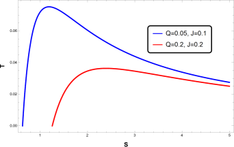
Figure 1: The Temperature (T) for Kerr-Sen black hole as a function of the entropy (S) for different values of $J$ and $Q$.

A close examination on the curve in the $S-T$ plane shows that the temperature $T$ is indeed a continuous function of the entropy. Thus, the possibility of a first-order phase transition is removed. Besides, one can notice from Fig.1 that the temperature decreases when the angular momentum and the charge does. However, it has been shown that the temperature vanishes at $S=2\pi J$ which could be linked with an extremal black hole solution. Then, the temperature exhibits a maximum point corresponding to its vanishing first derivative located at

$$S_{max}=\pi\sqrt{2\sqrt[3]{2J^{4}Q^{4}-8J^{6}}+4J^{2}}+\sqrt{4\pi^{2}J^{2}\left(\frac{Q^{2}}{\sqrt{\frac{1}{2}\sqrt[3]{2J^{4}Q^{4}-8J^{6}}+J^{2}}}+2\right)-2\pi^{2}\sqrt[3]{2J^{4}Q^{4}-8J^{6}}}.$$ (2.15)

Then, it goes to zero when $S$ goes to infinity. It is known that a second-order occurs at the point where the heat capacity exhibits a singularity. To get further insight into the thermodynamical behaviors of the Kerr-Sen black hole, we compute the semi-classical specific heat by using the relation $C_{J,Q}=T\left(\frac{\partial S}{\partial T}\right)$. This has been found to be

$$C_{J,Q}(S,Q,J)=\frac{2S(-4J^{2}\pi^{2}+S^{2})(4J^{2}\pi^{2}+S(2\pi Q^{2}+S))}{48J^{4}\pi^{4}-S^{4}+8J^{2}\pi^{2}S(4\pi Q^{2}+3S)}.$$ (2.16)

To investigate the associated behaviors, we plot the heat capacity as a function of the entropy in Fig.2.

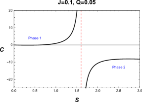
Figure 2: The heat capacity $(C)$ of Kerr-Sen black hole with respect to the entropy $(S)$ for fixed $J=0.1$ and $Q=0.05$.

It follows that this function involves a discontinuity at a critical value of the entropy given by $S_{c}=S_{max}=1.60199$. Such a point $S_{c}$ separates two branches associated with a small and large black hole transition. It can be seen also from Fig.2 that the heat capacity changes from a positive infinity to a negative infinity at $T=T_{c}=0.0874147$. An examination shows that there is an infinite divergence of the heat capacity that indicates a higher-order phase transition of the Kerr-Sen black hole. This critical transition can be treated using two different approaches which will be investigated in the next sections. The first one will be based on the Ehrenfest method. However, the second one will be conducted using a geometric way by adopting a new metric form inspired by the Gibbs free energy scaled by a conformal factor associated with the existence of extremal solutions.

3 Second-order phase transition of the Kerr-Sen black hole

In this section, we study a phase transition phenomena appearing in the Kerr-Sen black hole by using first the Ehrenfest scheme [22, 23, 24, 25, 26]. In particular, we will show that this black hole exhibits a second-order phase transition by adopting such a nice technique used for studying thermodynamical systems.

3.1 Kerr-Sen black hole behaviors from the Ehrenfest scheme

It is noted that the Ehrenfest scheme has been exploited to understand the nature of the phase transition, based on certain relations and equations. For such a black hole, twelve Ehrenfest equations are involved. They are grouped in Tab.1.

S fixed	$\Omega$ fixed	$\phi$ fixed
$-\left(\frac{\partial J}{\partial T}\right)_{S,Q}=\frac{({C_{J,Q}})_{2}-({C_{J,Q}})_{1}}{\Omega T(\alpha_{2}-\alpha_{1})}$	$\left(\frac{\partial J}{\partial T}\right)_{\Omega,Q}=\frac{\alpha_{2}-\alpha_{1}}{\kappa_{2}-\kappa_{1}}$	$\left(\frac{\partial J}{\partial T}\right)_{\phi,Q}=\frac{\phi({\alpha^{\prime}}_{2}-{\alpha^{\prime}}_{1})}{\Omega(\chi_{2}-\chi_{1})}$
$-\left(\frac{\partial J}{\partial Q}\right)_{S,T}=\frac{\phi({\alpha^{\prime}}_{2}-{\alpha^{\prime}}_{1})}{\Omega(\alpha_{2}-\alpha_{1})}$	$-\left(\frac{\partial J}{\partial Q}\right)_{\Omega,T}=\frac{\phi({\chi^{\prime}}_{2}-{\chi^{\prime}}_{1})}{\Omega(\kappa_{2}-\kappa_{1})}$	$-\left(\frac{\partial J}{\partial Q}\right)_{\phi,T}=\frac{\phi({\kappa^{\prime}}_{2}-{\kappa^{\prime}}_{1})}{\Omega(\chi_{2}-\chi_{1})}$
$-\left(\frac{\partial Q}{\partial J}\right)_{S,T}=\frac{\Omega(\alpha_{2}-\alpha_{1})}{\phi({\alpha^{\prime}}_{2}-{\alpha^{\prime}}_{1})}$	$-\left(\frac{\partial Q}{\partial J}\right)_{\Omega,T}=\frac{\Omega(\kappa_{2}-\kappa_{1})}{\phi({\chi^{\prime}}_{2}-{\chi^{\prime}}_{1})}$	$-\left(\frac{\partial Q}{\partial J}\right)_{\phi,T}=\frac{\Omega(\chi_{2}-\chi_{1})}{\phi({\kappa^{\prime}}_{2}-{\kappa^{\prime}}_{1})}$
$-\left(\frac{\partial Q}{\partial T}\right)_{S,J}=\frac{({C_{J,Q}})_{2}-({C_{J,Q}})_{1}}{\phi T({\alpha^{\prime}}_{2}-{\alpha^{\prime}}_{1})}$	$\left(\frac{\partial Q}{\partial T}\right)_{\Omega,J}=\frac{\Omega(\alpha_{2}-\alpha_{1})}{\phi({\chi^{\prime}}_{2}-{\chi^{\prime}}_{1})}$	$\left(\frac{\partial Q}{\partial T}\right)_{\phi,J}=\frac{{\alpha^{\prime}}_{2}-{\alpha^{\prime}}_{1}}{{\kappa^{\prime}}_{2}-{\kappa^{\prime}}_{1}}$

Table 1: Ehrenfest equations for the Kerr-Sen black hole.

The relevant thermodynamical coefficients are given by the following formulae

$$\begin{array}[]{ll}\alpha=-\frac{1}{\Omega}{\left(\frac{\partial\Omega}{\partial T}\right)}_{J,Q},\hskip 34.14322pt\kappa=\frac{1}{\Omega}{\left(\frac{\partial\Omega}{\partial J}\right)}_{T,Q},\hskip 34.14322pt\chi=\frac{1}{\Omega}{\left(\frac{\partial\phi}{\partial J}\right)}_{T,Q},\\[6.02249pt] \alpha^{\prime}=-\frac{1}{\phi}{\left(\frac{\partial\phi}{\partial T}\right)}_{J,Q},\hskip 34.14322pt\chi^{\prime}=\frac{1}{\Omega}{\left(\frac{\partial\Omega}{\partial Q}\right)}_{T,J},\hskip 34.14322pt\kappa^{\prime}=\frac{1}{\Omega}{\left(\frac{\partial\phi}{\partial Q}\right)}_{T,J}.\end{array}$$ (3.1)

As shown in Fig.2, the heat capacity $C_{J,Q}$ is discontinuous which is needed to reveal that the studied black hole system undergoes a second-order phase transition. This can be confirmed by examining the discontinuous behaviors of $\alpha$, $\kappa$, $\chi$, $\alpha^{\prime}$, $\kappa^{\prime}$ and $\chi^{\prime}$. To do so, one should compute such quantities. Using (2.12) and (2.13), we can express $\Omega$ and $\phi$ as a function of $S,J$ and $Q$. The calculations give

$$\Omega(S,Q,J)=\frac{2J\pi^{3/2}}{\sqrt{2\pi S^{2}Q^{2}+4J^{2}s\pi^{2}+S^{3}}},$$ (3.2)

$$\phi(S,Q,J)=\frac{\sqrt{S\pi}Q}{\sqrt{4J^{2}\pi^{2}+2\pi Q^{2}S+S^{2}}}.$$ (3.3)

By using (2.14), (3.2), and (3.3), the expressions of $\alpha$ and $\alpha^{\prime}$ can be written as

$$\alpha=-\frac{1}{\Omega}{\left(\frac{\partial\Omega}{\partial S}\right)}_{J,Q}{\left(\frac{\partial S}{\partial T}\right)}_{J,Q}=\frac{4S(4J^{2}\pi^{2}+S(4\pi Q^{2}+3S))\sqrt{S\pi(4J^{2}\pi^{2}+S(2\pi Q^{2}+S))}}{48J^{4}\pi^{4}-S^{4}+8J^{2}\pi^{2}S(4\pi Q^{2}+3S)}$$ (3.4)

$$\alpha^{\prime}=-\frac{1}{\phi}{\left(\frac{\partial\phi}{\partial S}\right)}_{J,Q}{\left(\frac{\partial S}{\partial T}\right)}_{J,Q}=\frac{4S(-4J^{2}\pi^{2}+S^{2})\sqrt{S\pi(4J^{2}\pi^{2}+S(2\pi Q^{2}+S))}}{48J^{4}\pi^{4}-S^{4}+8J^{2}\pi^{2}S(4\pi Q^{2}+3S)}.$$ (3.5)

Using the following equations

$${\left(\frac{\partial\Omega}{\partial J}\right)}_{T,Q}=\frac{{\left(\frac{\partial\Omega}{\partial J}\right)}_{S,Q}{\left(\frac{\partial T}{\partial S}\right)}_{J,Q}-{\left(\frac{\partial\Omega}{\partial S}\right)}_{J,Q}{\left(\frac{\partial T}{\partial J}\right)}_{S,Q}}{{\left(\frac{\partial T}{\partial S}\right)}_{J,Q}},\;\;{\left(\frac{\partial\phi}{\partial Q}\right)}_{T,J}=\frac{{\left(\frac{\partial\phi}{\partial Q}\right)}_{S,J}{\left(\frac{\partial T}{\partial S}\right)}_{J,Q}-{\left(\frac{\partial\phi}{\partial S}\right)}_{J,Q}{\left(\frac{\partial T}{\partial Q}\right)}_{S,J}}{{\left(\frac{\partial T}{\partial S}\right)}_{J,Q}}$$

we obtain

$$\kappa=\frac{(4J^{2}\pi^{2}+S^{2})^{2}}{J(48J^{4}\pi^{4}-S^{4}+8J^{2}\pi^{2}S(4\pi Q^{2}+3S))},$$ (3.6)

$$\kappa^{\prime}=\frac{48J^{4}\pi^{4}+24J^{2}\pi^{2}S^{2}-S^{4}}{Q(48J^{4}\pi^{4}-S^{4}+8J^{2}\pi^{2}S(4\pi Q^{2}+3S))}.$$ (3.7)

To get the expressions of the two final quantities, we exploit the formulae

$${\left(\frac{\partial\phi}{\partial J}\right)}_{T,Q}=\frac{{\left(\frac{\partial\phi}{\partial J}\right)}_{S,Q}{\left(\frac{\partial T}{\partial S}\right)}_{J,Q}-{\left(\frac{\partial\phi}{\partial S}\right)}_{J,Q}{\left(\frac{\partial T}{\partial J}\right)}_{S,Q}}{{\left(\frac{\partial T}{\partial S}\right)}_{J,Q}},\;\;{\left(\frac{\partial\Omega}{\partial Q}\right)}_{T,J}=\frac{{\left(\frac{\partial\Omega}{\partial Q}\right)}_{S,J}{\left(\frac{\partial T}{\partial S}\right)}_{J,Q}-{\left(\frac{\partial\Omega}{\partial S}\right)}_{J,Q}{\left(\frac{\partial T}{\partial Q}\right)}_{S,J}}{{\left(\frac{\partial T}{\partial S}\right)}_{J,Q}},$$

which gives the following relations

$$\chi=\frac{-4\pi QS(4J^{2}\pi^{2}+S^{2})}{48J^{4}\pi^{4}-S^{4}+8J^{2}\pi^{2}S(4\pi Q^{2}+3S)},$$ (3.8)

$$\chi^{\prime}=\frac{-8J\pi^{2}(4J^{2}\pi^{2}+S^{2})}{48J^{4}\pi^{4}-S^{4}+8J^{2}\pi^{2}S(4\pi Q^{2}+3S)}.$$ (3.9)

It is worth noting that $\alpha$, $\chi$, $\alpha^{\prime}$, $\kappa^{\prime}$ and $\chi^{\prime}$ share the same denominator being exactly the one of $C_{J,Q}(S,Q,J)$. Thus, such quantities diverge at the same critical value of the entropy. This critical behavior can be clearly seen from Fig.3 showing the variation of such quantities in terms of the entropy $S$.

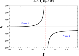
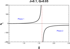
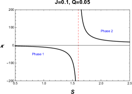
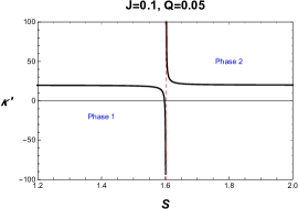
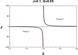
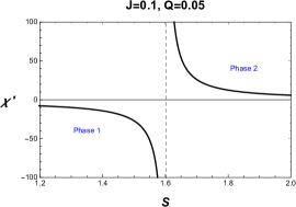
Figure 3: The variation of $\alpha$, $\kappa$, $\chi$, $\alpha^{\prime}$, $\kappa^{\prime}$ and $\chi^{\prime}$ with respect to the entropy for fixed values of $Q$ and $J$.

Precisely, it has been observed that all the computed quantities exhibit a discontinuity at the critical value $S_{c}=1.60199$ illustrated by the red dashed line. The obtained results show a genuine second-order phase transition for the Kerr-Sen black hole.

3.2 Validity of the Ehrenfest equations

Now we are in position to inspect the Ehrenfest equations organized in the table 1 by checking their validity. It is noted that for any second-order phase transition, the Ehrenfest equations should be satisfied at the critical point. Indeed, we consider first the Ehrenfest equations associated with the fixed entropy classes. Using (2.14), the left hand side of the first equation can be computed. This has been found to be

$$-\left(\frac{\partial J}{\partial T}\right)_{S,Q}=\frac{\left(\frac{S}{\pi}\left(4J^{2}\pi^{2}+S(2\pi Q^{2}+S\right)\right)^{3/2}}{J\left(4J^{2}\pi^{2}+S(4\pi Q^{2}+3S)\right)}.$$ (3.10)

To get the right hand side, we can use the expressions of $C_{J,Q}$ and $\alpha$ given in (2.16) and (3.4). Indeed, consider two points $S_{1}=S_{c}+\epsilon$ and $S_{2}=S_{c}-\epsilon$ $(\epsilon\ll 1)$ associated with phase 1 and phase 2, respectively of the curves given in Figs.2 and 3 and the corresponding $C_{J,Q}\mid_{S_{1}}={C_{(J,Q)_{1}}}$, $C_{J,Q}\mid_{S_{2}}={C_{(J,Q)_{2}}}$ and $\alpha\mid_{S_{1}}=\alpha_{1}$, $\alpha\mid_{S_{2}}=\alpha_{2}$, respectively. Putting $D(S,J,Q)=48J^{4}\pi^{4}-S^{4}+8J^{2}\pi^{2}S(4\pi Q^{2}+3S)$, the right hand side of the first Ehrenfest relation for fixed values of the entropy reads as

$$\frac{({C_{J,Q}})_{2}-({C_{J,Q}})_{1}}{\Omega T(\alpha_{2}-\alpha_{1})}=\frac{2S(-4J^{2}\pi^{2}+S^{2})(4J^{2}\pi^{2}+S(2\pi Q^{2}+S))}{\Omega T[4S(4J^{2}\pi^{2}+S(4\pi Q^{2}+3S))\sqrt{S\pi(4J^{2}\pi^{2}+S(2\pi Q^{2}+S))}]}\times\frac{\left(\frac{1}{D_{2}}-\frac{1}{D_{1}}\right)}{\left(\frac{1}{D_{2}}-\frac{1}{D_{1}}\right)}$$ (3.11)

where $D_{1}$ and $D_{2}$ denote the denominators associated with the phase 1 and 2, respectively. Using the expressions of $T$ and $\Omega$, the right hand side of the first Ehrenfest relation for a fixed value of the entropy is found to be

$$\frac{({C_{J,Q}})_{2}-({C_{J,Q}})_{1}}{\Omega T(\alpha_{2}-\alpha_{1})}=\frac{\left(\frac{S}{\pi}\left(4J^{2}\pi^{2}+S(2\pi Q^{2}+S\right)\right)^{3/2}}{J\left(4J^{2}\pi^{2}+S(4\pi Q^{2}+3S)\right)}$$ (3.12)

revealing that the first Ehrenfest equation is satisfied. Using similar calculations, we examine the second equation appearing in Tab.1. The left hand side of the second Ehrenfest equation can be written as

$$-\left(\frac{\partial J}{\partial Q}\right)_{S,T}=\frac{{\left(\frac{\partial T}{\partial Q}\right)}_{S,J}}{{\left(\frac{\partial T}{\partial J}\right)}_{S,Q}}.$$ (3.13)

Using the equations (2.14) and (3.13), we get

$$-\left(\frac{\partial J}{\partial Q}\right)_{S,T}=\frac{QS(S^{2}-4J^{2}\pi^{2})}{8J^{3}\pi^{3}+2J\pi S(4\pi Q^{2}+3S)}.$$ (3.14)

Exploiting the same procedure used in the verification of the first equation right hand side, we obtain

$$\frac{\phi({\alpha^{\prime}}_{2}-{\alpha^{\prime}}_{1})}{\Omega(\alpha_{2}-\alpha_{1})}=\frac{\phi[4S(-4J^{2}\pi^{2}+S^{2})\sqrt{S\pi(4J^{2}\pi^{2}+S(2\pi Q^{2}+S))}]}{\Omega[4S(4J^{2}\pi^{2}+S(4\pi Q^{2}+3S))\sqrt{S\pi(4J^{2}\pi^{2}+S(2\pi Q^{2}+S))}]}\times\frac{\left(\frac{1}{D_{2}}-\frac{1}{D_{1}}\right)}{\left(\frac{1}{D_{2}}-\frac{1}{D_{1}}\right)}.$$ (3.15)

Using (3.3) and (3.2), we arrive to

$$\frac{\phi({\alpha^{\prime}}_{2}-{\alpha^{\prime}}_{1})}{\Omega(\alpha_{2}-\alpha_{1})}=\frac{QS(S^{2}-4J^{2}\pi^{2})}{8J^{3}\pi^{3}+2J\pi S(4\pi Q^{2}+3S)}$$ (3.16)

which reveals clearly the validity of the Ehrenfest second equation at the critical point. For the third equation, the left hand side can be calculated using (2.14) and (3.17). Indeed, it is given by

$$-\left(\frac{\partial Q}{\partial J}\right)_{S,T}=\frac{{\left(\frac{\partial T}{\partial J}\right)}_{S,Q}}{{\left(\frac{\partial T}{\partial Q}\right)}_{S,J}}=\frac{8J^{3}\pi^{3}+2J\pi S(4\pi Q^{2}+3S)}{QS(S^{2}-4J^{2}\pi^{2})}.$$ (3.17)

Similar computations provide

$$\frac{\Omega(\alpha_{2}-\alpha_{1})}{\phi({\alpha^{\prime}}_{2}-{\alpha^{\prime}}_{1})}=\frac{\Omega[4S(4J^{2}\pi^{2}+S(4\pi Q^{2}+3S))\sqrt{S\pi(4J^{2}\pi^{2}+S(2\pi Q^{2}+S))}]}{\phi[4S(-4J^{2}\pi^{2}+S^{2})\sqrt{S\pi(4J^{2}\pi^{2}+S(2\pi Q^{2}+S))}]}\times\frac{\left(\frac{1}{D_{2}}-\frac{1}{D_{1}}\right)}{\left(\frac{1}{D_{2}}-\frac{1}{D_{1}}\right)}.$$ (3.18)

Using the expression of $\phi$ from (3.3) and $\Omega$ from (3.2), we find

$$\frac{\Omega(\alpha_{2}-\alpha_{1})}{\phi({\alpha^{\prime}}_{2}-{\alpha^{\prime}}_{1})}=\frac{QS(S^{2}-4J^{2}\pi^{2})}{8J^{3}\pi^{3}+2J\pi S(4\pi Q^{2}+3S)}.$$ (3.19)

This indicates the validity of such an Ehrenfest equation. For the last equation given in Tab.1 for a fixed entropy, we follow the same calculations by finding first the left hand side. Concretely, it has been found to be

$$-\left(\frac{\partial Q}{\partial T}\right)_{S,J}=\frac{2\left(S\left(4J^{2}\pi^{2}+S(2\pi Q^{2}+S\right)\right)^{3/2}}{\sqrt{\pi}QS\left(S^{2}-4J^{2}\pi^{2})\right)}.$$ (3.20)

For the right hand side, the calculation shows that it involves the same expression as the left handed side. Thus, we have

$$\frac{({C_{J,Q}})_{2}-({C_{J,Q}})_{1}}{\phi T({\alpha^{\prime}}_{2}-{\alpha^{\prime}}_{1})}=\frac{2\left(S\left(4J^{2}\pi^{2}+S(2\pi Q^{2}+S\right)\right)^{3/2}}{\sqrt{\pi}QS\left(S^{2}-4J^{2}\pi^{2})\right)}=-\left(\frac{\partial Q}{\partial T}\right)_{S,J}.$$ (3.21)

As expected, the remaining equations, given in Tab.1, can be examined using the same method. Instead of repeating the associated calculation, we give only the obtained results. For a fixed angular momentum, they are presented as follows

$$\frac{\alpha_{2}-\alpha_{1}}{\kappa_{2}-\kappa_{1}}=\frac{4SJ(4J^{2}\pi^{2}+S(4\pi Q^{2}+3S))\sqrt{S\pi(4J^{2}\pi^{2}+S(2\pi Q^{2}+S))}}{(4J^{2}\pi^{2}+S^{2})^{2}}={\left(\frac{\partial J}{\partial T}\right)}_{\Omega,Q},$$ (3.22)

$$\frac{\phi({\chi^{\prime}}_{2}-{\chi^{\prime}}_{1})}{\Omega(\kappa_{2}-\kappa_{1})}=\frac{4J\pi QS}{4J^{2}\pi^{2}+S^{2}}=-{\left(\frac{\partial J}{\partial Q}\right)}_{\Omega,T},$$ (3.23)

$$\frac{\Omega(\kappa_{2}-\kappa_{1})}{\phi({\chi^{\prime}}_{2}-{\chi^{\prime}}_{1})}=\frac{4J^{2}\pi^{2}+S^{2}}{4J\pi QS}=-{\left(\frac{\partial Q}{\partial J}\right)}_{\Omega,T},$$ (3.24)

$$\frac{\Omega(\alpha_{2}-\alpha_{1})}{\phi({\chi^{\prime}}_{2}-{\chi^{\prime}}_{1})}=\frac{Q(4J^{2}\pi^{2}+S^{2})}{\sqrt{\frac{S}{\pi}(4J^{2}\pi^{2}+S(2\pi Q^{2}+S))}}={\left(\frac{\partial Q}{\partial T}\right)}_{\Omega,J}.$$ (3.25)

For a fixed electric potential, the Ehrenfest equations are also verified

$$\frac{\phi({\alpha^{\prime}}_{2}-{\alpha^{\prime}}_{1})}{\Omega(\chi_{2}-\chi_{1})}=\frac{S(4J^{2}\pi^{2}-S^{2})\sqrt{S(4J^{2}\pi^{2}+S(2\pi Q^{2}+S))}}{2J\pi^{3/2}(4J^{2}\pi^{2}+S^{2})}={\left(\frac{\partial J}{\partial T}\right)}_{\phi,Q},$$ (3.26)

$$\frac{\phi({\kappa^{\prime}}_{2}-{\kappa^{\prime}}_{1})}{\Omega(\chi_{2}-\chi_{1})}=-\frac{48J^{4}\pi^{4}+24J^{2}\pi^{2}S^{2}-S^{4}}{32J^{3}\pi^{4}Q+8J\pi^{2}QS^{2}}=-{\left(\frac{\partial J}{\partial Q}\right)}_{\phi,T},$$ (3.27)

$$\frac{\Omega(\chi_{2}-\chi_{1})}{\phi({\kappa^{\prime}}_{2}-{\kappa^{\prime}}_{1})}=-\frac{32J^{3}\pi^{4}Q+8J\pi^{2}QS^{2}}{48J^{4}\pi^{4}+24J^{2}\pi^{2}S^{2}-S^{4}}=-{\left(\frac{\partial Q}{\partial J}\right)}_{\phi,T},$$ (3.28)

$$\frac{{\alpha^{\prime}}_{2}-{\alpha^{\prime}}_{1}}{{\kappa^{\prime}}_{2}-{\kappa^{\prime}}_{1}}=\frac{4QS(-4J^{2}\pi^{2}+S^{2})\sqrt{S\pi(4J^{2}\pi^{2}+S(2\pi Q^{2}+S))}}{48J^{4}\pi^{4}+24J^{2}\pi^{2}S^{2}-S^{4}}={\left(\frac{\partial Q}{\partial T}\right)}_{\phi,J}.$$ (3.29)

It has been shown that Prigogine- Defay (PD) ratio $\Pi$ can be considered as a tool to measure the deviation from the second Ehrenfest equation [27]. Performing numerical calculations from eqs.(3.12) and (3.23), it has been found to be

$$\Pi=\frac{\Delta C_{J,Q}\Delta\kappa}{T_{c}\Omega_{c}(\Delta\alpha)^{2}}=1.$$ (3.30)

Since all the Ehrenfest equations presented in Tab.1 are verified, we can now confirm the existence of a second-order phase transition for the Kerr-Sen black hole. Note that this matches perfectly with the second-order equilibrium transition discussed in [26, 28, 29].

To consolidate this result, we shall explore the geothermodynamics by proposing a new metric form derived from the Gibbs free energy scaled by a conformal factor associated with the existence of extremal solutions.

4 Kerr-Sen black hole geothermodynamics

In this section, we reconsider the investigation of the geothermodynamics, of such a black hole, relying on singular behaviors of certain thermodynamical quantities including the heat capacity. The latter is relevant in the determination of the nature of the black hole phase transitions, since it involves various interesting thermodynamical properties. To unveil such properties, the thermodynamical geometry of the Kerr-Sen black hole has been approached by focusing on the thermodynamical geometric curvature. Several metrics could be used to approach such a quantity. However, here, we can explore an alternative road. Inspired by the Hessian matrix of several free energies generated from the Legendre transformation of $M$, we adopt a new metric form derived from the Gibss free energy [30]. Concretely, we introduce a conformal factor $\frac{1}{T}$ motivated by extremal solutions being absent in known approaches. Exploiting the Gibbs free energy $G$, we can write

$$dG=-SdT+\phi dQ+\Omega dJ.$$ (4.1)

Implementing a conformal factor $\frac{1}{T}$, we obtain

$$\frac{1}{T}dG=\frac{1}{T}\left(-SdT+\phi dQ+\Omega dJ\right).$$ (4.2)

It follows that the conformal Gibbs free energy metric can be written as

$$ds^{2}_{G}=\frac{1}{T}\left(-dTdS+d\phi dQ+d\Omega dJ\right).$$ (4.3)

Within the natural variables $T$, $Q$ and $J$, it is convenient to trade the temperature by the entropy $S$. The resulting new representation of the metric takes the following form

$$ds^{2}_{G}=g_{SS}dS^{2}+g_{QQ}dQ^{2}+g_{JJ}dJ^{2}+2g_{QJ}dQdJ.$$ (4.4)

With the use of this metric, we try to check the second-order phase transition point. Thus, the scalar curvature can be expressed in the following way

$$\mathfrak{R}_{G}=\frac{\mathfrak{N}_{G}}{\mathfrak{D}_{G}},$$ (4.5)

where the denominator is found to be

$$\mathfrak{D}_{G}=S(2J\pi-S)(2J\pi+S)(2\pi Q^{2}+S)^{2}(4J^{2}\pi^{2}+S^{2})(4J^{2}\pi^{2}+2\pi Q^{2}S+S^{2}),$$ (4.6)

$$(48J^{4}\pi^{4}-S^{4}+8J^{2}\pi^{2}S(4\pi Q^{2}+3S))^{2},$$

while the term $\mathfrak{N}_{G}$, having a complicated form, is omitted since it is not revelent in the present discussion. It is worth noting that the proposed metric gives a rather simple form of the scalar curvature. Besides, the resulting scalar curvature has the same denominator as the quantities (2.16) and (3.1). This shows that the latter may also exhibit a discontinuity at the critical point $S_{c}=1.60199$ confirming the existence of a second-order phase transition. To visualise such a result, we illustrate the scalar curvature in Fig.4 as a function of the entropy.

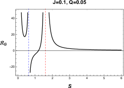
Figure 4: Scalar curvature as a function of the entropy (S). The red dashed line represents the critical point at which $\mathfrak{R}_{G}$ goes to infinity. While, the blue one is associated with the extremal black hole solution.

It follows from this figure that the scalar is indeed discontinuous at $S_{c}$ (the red dashed line) and at $S=2\pi J$ (the blue dashed line). This not only supports the result obtained in the previous section but also pushes one to investigate the associated scalings laws and critical exponents.

5 Scaling laws and critical exponents

In this section, we investigate the scaling laws and the critical exponents at the obtained critical point for the Kerr-Sen black hole. In the elaboration of critical phenomena, one can meet with three kinds of susceptibilities related to the heat capacity $C_{A}$, the moment of inertia $(I_{B})$ and the electric capacitance $(K_{c})$ defined as

$$C_{A}=-\beta^{2}\left(\frac{\partial M}{\partial\beta}\right)_{A},\quad I_{B}=\beta\left(\frac{\partial J}{\partial\left(\beta\Omega\right)}\right)_{B},\quad K_{C}=\beta\left(\frac{\partial Q}{\partial\left(\beta\phi\right)}\right)_{C}.$$ (5.1)

Here, $\beta$ is the inverse of the temperature and the set $\left\{A,B,C\right\}$ denotes the fixed quantities [31]. These quantities representing different exchange modes (i.e thermal, electrical and mechanical) show a behavioral divergence providing a phase transition. It is noted that other propositions have been conducted for the phase transitions at the extremal limit, being a point of a second-order transition, when $M=a+b$ based on the divergence of thermal fluctuations. Precisely, it has been remarked that these fluctuations can be linked to the divergence of (5.1). Before going ahead, it is convenient to re-write certain needed thermodynamical quantities. In particular, they are listed as follows

$$S_{\pm}=\frac{A_{\pm}}{4}=\pi\left[2M^{2}-Q^{2}\pm\sqrt{\left(2M^{2}-Q^{2}\right)^{2}-4J^{2}}\right],$$ (5.2)

$$T_{\pm}=\frac{\pm\sqrt{\left(2M^{2}-Q^{2}\right)^{2}-4J^{2}}}{M\times A_{\pm}}=\beta^{-1},$$ (5.3)

$$\Omega_{\pm}=\frac{4\pi J}{MA_{\pm}},\quad\phi_{\pm}=\frac{4\pi Qr_{h}}{A_{\pm}}.$$ (5.4)

It is noted that the entropy $S(M,J,Q)$ is a generalized homogeneous function since one has
$S(\sqrt{\lambda}M,\lambda J,\sqrt{\lambda}Q)=\lambda S(M,J,Q)$. The response coefficients are related to the susceptibilities via the following relations

$$\overline{\chi}_{1}\equiv\left(\frac{\partial^{2}S}{\partial M^{2}}\right)_{JQ}=-\frac{\beta^{2}}{C_{JQ}},$$ (5.5)

$$\overline{\chi}_{2}\equiv\left(\frac{\partial^{2}S}{\partial J^{2}}\right)_{MQ}=-\frac{\beta}{I_{MQ}},$$ (5.6)

$$\overline{\chi}_{3}\equiv\left(\frac{\partial^{2}S}{\partial Q^{2}}\right)_{MJ}=-\frac{\beta}{K_{MJ}}.$$ (5.7)

Near the critical points, these quantities obey certain power laws. To derive such laws, we should define the following order parameters $\eta_{M}=\beta_{+}-\beta_{-}$, $\eta_{J}=(\beta\Omega)_{+}-(\beta\Omega)_{-}$ and $\eta_{Q}=(\beta\phi)_{+}-(\beta\phi)_{-}$. It is worth noting that these quantities do not go to zero at the critical point. However, they diverge since the inverse of the black hole temperature does. In this regime, we also need to define the following terms $M=M_{X}(1+\epsilon_{M}),J=J_{X}(1-\epsilon_{J}),Q=Q_{X}(1-\epsilon_{Q}$), where $M_{X},J_{X}$ and $Q_{X}$ represent the mass, the angular momentum, and the charge at the extremal limit, respectively and $\epsilon$ is associated with small parameter deviations. Some of the relevant scaling laws are given by

$$\overline{\chi}_{1}\sim\epsilon_{M}^{-\alpha}(J=0\,\text{or}\,Q=0),$$ (5.8)

$$\overline{\chi}_{2}\sim\epsilon_{M}^{-\gamma}(Q=0),$$ (5.9)

$$\eta_{J}\sim\epsilon_{M}^{\beta}(Q=0),$$ (5.10)

$$\eta_{J}\sim\epsilon_{M}^{\delta-1}(Q\neq 0).$$ (5.11)

Using the definition of $\overline{\chi}_{1}$ in the extremal limit where $M=\sqrt{J+Q^{2}/2}(1+\epsilon_{M})$ and taking $Q=0$, we find

$$\overline{\chi}_{1}\approx\frac{4\pi}{\epsilon_{M}^{3/2}(\epsilon_{M}+2)^{3/2}(\epsilon_{M}(\epsilon_{M}+2)+2)^{3/2}}$$ (5.12)

$$\times\left[-2+\epsilon_{M}^{3/2}(\epsilon_{M}+2)\left((\epsilon_{M}+2)\sqrt{\epsilon_{M}}\left(\epsilon_{M}^{2}+2\epsilon_{M}+\sqrt{\epsilon_{M}}\sqrt{\epsilon_{M}+2}\sqrt{\epsilon_{M}(\epsilon_{M}+2)+2}+3\right)+2\sqrt{\epsilon_{M}+2}\sqrt{\epsilon_{M}(\epsilon_{M}+2)+2}\right)\right].$$

Thus, we obtain $\overline{\chi}_{1}\propto\epsilon_{M}^{-3/2}.$ Using similar road calculations, we get

$$\overline{\chi}_{2}\approx-\frac{2\pi(\epsilon_{M}+1)^{4}}{J\left(\epsilon_{M}^{4}+4\epsilon_{M}^{3}+6\epsilon_{M}^{2}+4\epsilon_{M}\right)^{3/2}},$$ (5.13)

which shows that $\overline{\chi}_{2}\propto\epsilon_{M}^{-3/2}$. For the third equation, we obtain

$$\eta_{J}\approx-\frac{4\pi}{\sqrt{\epsilon_{M}^{4}+4\epsilon_{M}^{3}+6\epsilon_{M}^{2}+4\epsilon_{M}}},$$ (5.14)

revealing that one has $\eta_{J}\propto\epsilon_{M}^{-1/2}$. Identical computations are performed for the last equation. The critical exponents for the Kerr-Sen black hole are therefore summarized as follows

$$\alpha=\frac{3}{2},\,\,\,\gamma=\frac{3}{2},\,\,\,\beta=-\frac{1}{2},\,\,\,\delta=-2.$$ (5.15)

From these critical exponents, we find the equalities related to the scaling laws of the first kind

$$\alpha+2\beta+\gamma=2,\quad\beta\left(\delta-1\right)=\gamma.$$ (5.16)

This matches perfectly with the result of [31] where the same relations have been obtained for the Kerr-Newman black hole.

6 Conclusions

In this work, we have investigated the phase transitions of the Kerr-Sen black hole engineered from the heterotic superstring theory. In particular, we have computed the involved thermodynamical quantities. It has been shown that the phase transition is characterized by divergences in the specific heat and other quantities near the critical points. Using the Ehrenfest scheme, we have inspected the nature of the phase transitions. Concretely, we have analytically verified the validity of such equations near the critical point. We have shown that the phase transition corresponding to the divergence in the heat capacity at the critical point is in fact a second-order equilibrium one. To support such a finding, we have approached the Kerr-Sen black hole geothermodynamics by adopting a new metric form derived from the Gibbs free energy scaled by a conformal factor inspired by the singularity associated with extremal solutions. This geometric method recovers similar behaviors. At the end, we have obtained the involved scaling behaviors at the critical point.
This work comes up with some open questions. It will be interesting to extend this investigation by considering backgrounds with a non zero cosmological constant built recently in [32]. Motivated by the black hole observational aspect such the gravitational waves and black hole image, a second investigation could concern optical properties from different backgrounds, including dark sectors. We leave these questions for future works.

References

- [1] S. W. Hawking, Black holes in general relativity, Communications in Mathematical Physics 25(2) (1972) 152-166.
- [2] J. B. Hartle, T. Dray, Gravity: An introduction to Einsteins general relativity, Amer. J. Phys. 71 (2003) 1086-1087.
- [3] J. L. Zhang, R. G. Cai, H. Yu, Phase transition and thermodynamical geometry for Schwarzschild AdS black hole in spacetime, J. High Ener. Phys. 2 (2015) 143.
- [4] A. Belhaj, M. Chabab, H. El Moumni, K. Masmar, M. B. Sedra, On thermodynamics of AdS black holes in M-theory, Eur. Phys. J. C 76(2) (2016) 73.
- [5] A. Belhaj, A. El Balali, W. El Hadri, Y. Hassouni, E. Torrente-Lujan, Phase Transitions of Quintessential AdS Black Holes in M-theory/Superstring Inspired Models, arXiv:2004.10647.
- [6] H. J. Boonstra, B. Peeters, K. Skenderis, Branes And Anti-de Sitter Space-times, Prog. Phys. 47(1-3) (1999) 109-116.
- [7] A. Sen, Rotating charged black hole solution in heterotic string theory, Phys. Rev. Lett.69(7) (1992) 1006.
- [8] S. Liebes Jr, Gravitational lenses, Phys. Rev. B835 (1964)133 .
- [9] L. Ming-Jian, Temperature and thermodynamic geometry of the Kerr-Sen black hole, Chin. Phys. B. 20.2 (2011) 020404.
- [10] X. G. Lan, J. Pu, Observing the contour profile of a Kerr-Sen black hole, Mod. Phys. Lett. A. 33.17 (2018) 1850099.
- [11] A. Belhaj, M. Benali, A. El Balali, H. El Moumni, S-E. Ennadifi, Deflection Angle and Shadow Behaviors of Quintessential Black Holes in arbitrary Dimensions, arXiv:2006.01078.
- [12] K. Akiyama et al. [Event Horizon Telescope Collaboration], First M87 Event Horizon Telescope Results. I. The Shadow of the Supermassive Black Hole, Astrophys. J. 875 (2019) no.1, L1.
- [13] A. Belhaj, M. Chabab, H. El Moumni and M. B. Sedra, On thermodynamics of AdS black holes in arbitrary dimensions, Chin. Phys. Lett. 29 (2012) 100401.
- [14] A. Belhaj, M. Chabab, H. El Moumni, L. Medari and M. B. Sedra, The thermodynamical behaviors of KerrNewman AdS black holes, Chin. Phys. Lett. 30 (2013) 090402.
- [15] S. W. Hawking, Black holes and thermodynamics, Phys. Rev. D 13(2) (1976) 191.
- [16] J. Xu, L. M. Cao, Y. P. Hu, P-V criticality in the extended phase space of black holes in massive gravity, Phys. Rev. D 91(12) (2015) 124033.
- [17] A. Belhaj, A. El Balali, W. El Hadri, M. A. Essebani, M. B.Sedra , A. Segui, Kerr-AdS Black Hole Behaviors from Dark Energy, International Journal of Modern Physics D, doi: 10.1142/S0218271820500698.
- [18] Y. Wu and W. Xu, Effet of dark energy on Hawking-Page transition, Phys. Dark Univ. 27 (2020) 100470.
- [19] A. Belhaj, A. El Balali, W. El Hadri, H. El Moumni, M. B. Sedra, Dark energy effects on charged and rotating black holes, Eur. Phys. J. Plus 134(9) (2019) 422.
- [20] J.X. Mo, W. B. Liu. Ehrenfest scheme for PV criticality in the extended phase space of black holes, Phys. Lett. B 727.1-3 (2013) 336-339.
- [21] A. Lala, D. Roychowdhury, Ehrenfest’s scheme and thermodynamic geometry in Born-Infeld AdS black holes, Phys. Rev. D 86 8 (2012) 084027.
- [22] H. E. Stanley, Introduction to phase transitions and critical phenomena, Oxford University Press, New York (1987).
- [23] M. W. Zemansky and R. H. Dittman, Heat and thermodynamics: an intermediate textbook, McGraw-Hill (1997).
- [24] R. Banerjee, S. K. Modak and S. Samanta, Glassy phase transition and stability in black holes, Eur. Phys. J. C 70 (2010)317.
- [25] R. Banerjee, S. Ghosh and D. Roychowdhury, New type of phase transition in Reissner Nordström–AdS black hole and its thermodynamic geometry, Phys. Lett.B 696 (2011) 156.
- [26] T. M. Nieuwenhuizen, Ehrenfest relations at the glass transition: solution to anold paradox, Phys. Rev. Lett. 79(1997)1317-1320.
- [27] R. Banerjee, D. Roychowdhury, Thermodynamics of phase transition in higher dimensional AdS black holes, JHEP11(2011)004.
- [28] H. Xu, W. Xu and L. Zhao, Extended phase space thermodynamics for third order Lovelock black holes in diverse dimensions, Eur. Phys. J. C 74, no.9, (2014)3074, arXiv:1405.4143.
- [29] A. Belhaj, M. Chabab, H. EL Moumni, K. Masmar and M. B. Sedra, Ehrenfest scheme of higher dimensional AdS black holes in the third-order Lovelock–Born–Infeld gravity, Int. J. Geom. Meth. Mod. Phys. 12, no.10, (2015)1550115, arXiv:1405.3306.
- [30] H. Liu, H. Lu, M. Luo, K.N. Shao, Thermodynamical metrics and black hole phase transitions, JHEP 1012 (2010) 054.
- [31] O. Kaburaki, Scaling laws at the critical point on black hole equilibrium series, Phys. Lett. A 217 (1996)315-320.
- [32] D. Wu, P. Wu, H. Yu, S-Q. Wu, Are ultra-spinning Kerr-Sen-AdS4 black holes always super-entropic?, arXiv:2007.02224.