Numerical scheme for solving the nonuniformly forced cubic and quintic Swift-Hohenberg equations strictly respecting the Lyapunov functional

Abstract

Computational modeling of pattern formation in nonequilibrium systems is a fundamental tool for studying complex phenomena in biology, chemistry, materials and engineering sciences. The pursuit for theoretical descriptions of some among those physical problems led to the Swift-Hohenberg equation (SH3) which describes pattern selection in the vicinity of instabilities. A finite differences scheme, known as Stabilizing Correction (Christov & Pontes; 2001 DOI: 10.1016/S0895-7177(01)00151-0), developed to integrate the cubic Swift-Hohenberg equation in two dimensions, is reviewed and extended in the present paper. The original scheme features Generalized Dirichlet boundary conditions (GDBC), forcings with a spatial ramp of the control parameter, strict implementation of the associated Lyapunov functional, and second order representation of all derivatives. We now extend these results by including periodic boundary conditions (PBC), forcings with Gaussian distributions of the control parameter and the quintic Swift-Hohenberg (SH35) model. The present scheme also features a strict implementation of the functional for all test cases. A code verification was accomplished, showing unconditional stability, along with second order accuracy in both time and space. Test cases confirmed the monotonic decay of the Lyapunov functional and all numerical experiments exhibit the main physical features: highly nonlinear behaviour, wavelength filter and competition between bulk and boundary effects.

1 Introduction

Understanding the selection and orientation mechanisms of spatial structures, their symmetries and instabilities is a major theme of theoretical and experimental research in modeling of self-organization phenomena. Nowadays, spatiotemporal organization is recognized to be related to several technological problems in chemistry [1], nonlinear optics [2], and materials science [3, 4, 5]. For computational material science and engineering a long-term goal is to adapt these models and appropriate numerical techniques to multiple scales and increasingly larger scale systems in order to achieve predictive capabilities [6, 7, 8, 9].

The pursuit for understanding self-organization in transport phenomena problems led to the Swift-Hohenberg (SH) equation [10]. It is a widely accepted model for describing pattern formation in many physical systems presenting symmetry breaking instabilities, such as the emergence of convection rolls in a thin layer of fluid heated from below. It first appeared in the framework of Bénard thermal convection between two “infinite” horizontal surfaces with distinct temperatures, where J. Swift and P. Hohenberg [10] performed a reduction of the full dynamics, led by the Boussinesq equations, into a dynamics governed by the most relevant slow modes represented by an order parameter. Such reduction can also be carried out for reaction-diffusion systems where a similar model is obtained with an additional quadratic nonlinearity (SH23) [3, 11]. Later, an extension of the original Swift-Hohenberg equation (SH3) was proposed with the introduction of a destabilizing cubic term and a quintic one. The resulting quintic SH equation (SH35) admits the coexistence of stable uniform and structured solutions, leading to an influx of studies on localized structures and snaking through the SH equation [12, 13].

Roughly speaking, the SH equation has three basic pattern-forming mechanisms, related to each term of the equation. The first is a control parameter (e.g. distance to temperature threshold in the Rayleigh-Bénard convection) in the linear part of the equation, which will be addressed to as a forcing parameter. It represents how far from the onset of the instability the system is. The second is the wavelength filter that contains all the equation spatial derivatives, and leads to wavelength selection in the resulting patterns. The third one is the nonlinear part of the equation, whose terms promote interactions between modes involved in the dynamics. For example, in the SH3 the cubic term is responsible for saturating the linear growth. Meanwhile, in the SH35 the cubic term destabilizes the dynamics leaving the quintic one responsible for the saturation. Some generalizations of theses mechanisms appear in literature, such as theoretical works exploring nonuniform forcings in the Rayleigh-Bénard convection [14, 15].

The SH equation admits a potential, formally known as the Lyapunov functional, from which the dynamical equation governing the evolution of the order parameter can be derived. In recent years, this potential nature has been exploited in condensed matter as a physical feature associated with the system’s free energy, used to describe patterning in materials. In this context, the SH dynamics is part of the phase-field theory, which was developed from statistical mechanics principles, and whose goal is to obtain governing equations for microstructure evolution; it connects thus thermodynamic and kinetic properties with microstructure via a mathematical formalism [5, 7, 16, 17]. The phase-field theory is a descendant of the van der Waals, Cahn-Hilliard and Landau type classical field theoretical approaches, originating from a single order parameter gradient theory of Langer [18, 19]. In this theory, the local state of matter is characterized by an order parameter $\psi(\mathbf{x},t)$, the phase-field variable, which monitors the transition between phases of distinct order of property. It can represent the structural order parameter that measures local crystallinity, the composition of a phase, the degree of a molecular ordering, among others. In the case of the phase-field crystal (PFC) approach, a conserved dynamics is assumed for this order parameter. Although this formalism will not be addressed in this paper, many recent theoretical and numerical works [20, 21, 22] are interested on conserved SH forms for PFC applications

Naturally, these applications led to the development of a series of mathematical and numerical methods concerned with the study of the SH equation In the beginning of this endeavor, Greenside & Coughran Jr. (1984) [23] achieved relevant results through a finite differences approach by using a backward Euler time-integration scheme with rigid [24, 25] and periodic boundary conditions (PBC). Those types of boundary conditions were also explored by Manneville (1990)[26] and Cross (1994)[27]. These works considered uniform control parameters. Other authors employed nonuniform distributions (ramps and Gaussians) for the control parameter and presented very interesting results as well, displaying rich competition between bulk and boundary effects. In particular, ramped control parameters mostly appears in the context of rigid boundaries [28, 29], which will be addressed here as Generalized Dirichlet boundary conditions (GDBC), following [28, 30, 29].

Besides finite differences, spectral methods have become largely employed due to their highly spatial accurate solutions [31, 32, 33]. They usually treat the nonlinear terms explicitly in the physical space, and therefore are called pseudo-spectral methods. Fully explicit schemes lead to severe stability restrictions on the time step, due to the the fourth-order nonlinear partial differential equation originated from the non-conserved dynamics. In the case of the PFC applications, the conserved dynamics is governed by a six-order nonlinear partial differential equation, which is even more restrictive for the time step selection. While PFC is not a subject of this work, our proposed scheme can be readily translated into a numerical framework for many PFC problems.

The present article is a continuation of the work presented by Christov & Pontes (2002)[30], where the authors employed a finite differences scheme for solving the cubic Swift-Hohenberg equation (SH3) in two dimensions, with uniform forcing, GDBC, and strict implementation of the associated functional. This scheme, known as Stabilizing Correction [34, 35], was originally introduced by Douglas & Rachford in the context of the temperature equation, and has also been adopted for solving fourth-order nonlinear differential equations similar to SH, such as the Kuramoto-Sivashinsky equation [36]. Here, we expand the previous study on the SH equation [30] for additional nonlinearities, boundary conditions and a spatially dependent control parameter. This includes the quintic SH35 with both GDBC and PBC, nonuniform Gaussian distributions of the control parameter in addition to ramps, and also a strict implementation of the associated Lyapunov functional. The scheme features a semi-implicit time splitting with second order representation of time and space derivatives. It is pertinent to point out that operator splitting methods enable parallel code processing implementation, which allows faster simulations. The usage of sparse matrices also plays a huge role in lowering computational cost in the simulations, and therefore it was implemented in the present work.

A code verification is performed to confirm the unconditional stability of the scheme, along with its second order convergence in both time and space. Since nonlinear partial differential equations such as SH do not have easily accessible analytical solutions, the adopted method to verify the order of accuracy of the code is the method of manufactured solutions (MMS). It provides a convenient way of verifying the implementation of nonlinear numerical algorithms, since we can use an artificial (manufactured) solution for this purpose [37, 38, 36].

This paper is organized as follows. Section 2 briefly discusses the properties of the SH equation and the numerical scheme for solving the cubic and quintic versions of the equation with GDBC and PBC, nonuniform forcings, and the discrete implementation of the associated Lyapunov functional. Section 3 contains all verification procedures adopted. Section 4 presents the numerical experiments. The results are grouped in three parts; the first one showing the steady state patterns obtained in ten simulations with the SH3 equation; the second one showing six simulations with the SH35 and the last one with discussions. Section 5 contains the final remarks of the work.

2 Mathematical modelling and numerical scheme

The mathematical description of the dimensionless governing equations is briefly discussed in the start of this section. Next, the details of the numerical framework are discussed as an extension of Christov & Pontes (2002)[30] work. For both SH3 and SH35 discretizations, a finite difference semi-implicit scheme of second order accuracy in time and space is presented. Finally, the choices for the operator splitting method, spatial discretizations and mesh types are clarified.

2.1 Governing equations

The SH equation has the so-called gradient dynamics, which means there is a potential function of the order parameter $\psi\left({\bf x},t\right)$, (known as a Lyapunov functional), that has the property of decreasing monotonically during the evolution [30]. This dynamic equation can be derived from the $L^{2}$-gradient flow of the Lyapunov energy functional:

$$\mathcal{F}[\psi] \vcentcolon=\int_{\Omega}{d\mathbf{x}}\dfrac{1}{2}\left\{-{\epsilon(\mathbf{x})}\psi^{2}+{\alpha}\left[(q_{0}^{2}+\nabla^{2})\psi\right]^{2}-\dfrac{\beta}{2}\psi^{4}+\dfrac{\gamma}{3}\psi^{6}\right\};$$ (1)

$$\dfrac{\partial\mathcal{F}[\psi]}{\partial t} =-\int_{\Omega}{d\mathbf{x}}\left(\dfrac{\partial\psi}{\partial t}\right)^{2}\leq 0.$$ (2)

where $\Omega$ represents the domain whose size is commensurate with the length scales of the patterns. We consider a regular domain $\Omega:\{x\in[0,L_{x}]$, $y\in[0,L_{y}]\}$. Equation (2) denotes the nonincreasing behavior of the Lyapunov functional, which monotonically decreases until steady state is reached [30]. By taking the variational derivative of Eq. (1) in $L^{2}$ norm, the Swift-Hohenberg equation is obtained:

$$\centering\dfrac{\partial\psi}{\partial t}=-\mu=\epsilon(\mathbf{x})\psi-\alpha\left(q_{0}^{2}+\nabla^{2}\right)^{2}\psi+\beta\psi^{3}-\gamma\psi^{5}\,,\@add@centering$$ (3)

where $\mu={\delta\mathcal{F}[\psi]}/{\delta\psi}$ is the chemical potential. As discussed by Christov et al. [30, 28], the appropriate boundary conditions for this system should consider only production and dissipation in the bulk and not on the boundary ($\partial\Omega$). This can be achieved by assuming Generalized Dirichlet boundary conditions (GDBC), $v=\partial v/\partial n=0$, where $n$ stands for the outward normal direction to the boundary. Periodic boundary conditions (PBC) will also be addressed in this work, since the absence of boundaries also leads boundary ($\partial\Omega$) integrals to vanish.

We expand Eq. (3) by considering the following laplacian operator in cartesian coordinates: $\nabla^{2}\equiv{\partial^{2}}/{\partial x^{2}}+{\partial^{2}}/{\partial y^{2}}$, we have:

$$\dfrac{\partial\psi}{\partial t}= \;\epsilon(\mathbf{x})\psi-\alpha q_{0}^{4}\psi-2\alpha q_{0}^{2}\nabla^{2}\psi-\alpha\nabla^{4}\psi+\beta\psi^{3}-\gamma\psi^{5}$$ (4)

$$= \;\epsilon(\mathbf{x})\psi-\alpha q_{0}^{4}\psi-2\alpha q_{0}^{2}\dfrac{\partial^{2}\psi}{\partial x^{2}}-2\alpha q_{0}^{2}\dfrac{\partial^{2}\psi}{\partial y^{2}}-\alpha\dfrac{\partial^{4}\psi}{\partial x^{4}}-2\alpha\dfrac{\partial^{4}\psi}{\partial x^{2}\partial y^{2}}-\alpha\dfrac{\partial^{4}\psi}{\partial y^{4}}+\beta\psi^{3}-\gamma\psi^{5}.$$

Table 1: Parameters assumed for the governing equations studied in this work.

Equation	Nonlinearity	$\alpha$	$\beta$	$\gamma$	$q_{0}$
SH3	cubic	1	-1	0	1
SH35	quintic	1	1	1	1

By using the parameters and values of Table 1 in Eq. (3), we define the forms of the SH3 and SH35. The discretization of these governing equations is described in the following subsection.

2.2 The target scheme

In order to construct a Crank-Nicolson second order in time numerical scheme, we adopt the following representation proposed by Christov and Pontes (2002) [30] for the time derivative of Eq. (3), where the RHS is evaluated at the middle of the time step $\Delta t$. The updated scheme, now including a quintic term takes the form:

$$\dfrac{\psi^{n+1}-\psi^{n}}{\Delta t}\,=\,-\mu^{n+1/2}\,=\, \left[\epsilon(\mathbf{x})-\alpha q_{0}^{4}-2\alpha q_{0}^{2}\dfrac{\partial^{2}}{\partial x^{2}}-2\alpha q_{0}^{2}\dfrac{\partial^{2}}{\partial y^{2}}-\alpha\dfrac{\partial^{4}}{\partial x^{4}}-2\alpha\dfrac{\partial^{4}}{\partial x^{2}\partial y^{2}}-\alpha\dfrac{\partial^{4}}{\partial y^{4}}\right.$$

$$\left.+\beta\dfrac{\left(\psi^{n+1}\right)^{2}+\left(\psi^{n}\right)^{2}}{2}-\gamma\dfrac{\left(\psi^{n+1}\right)^{4}+\left(\psi^{n}\right)^{4}}{2}\right]\left(\dfrac{\psi^{n+1}+\psi^{n}}{2}\right).$$ (5)

The superscript $(n+1)$ refers to the next time to be evaluated and $n$, to the current one. The parameter values for $\alpha$, $\beta$, $\gamma$ and $q_{0}$ are chosen according to Table 1. The RHS terms of Eq. (5) are grouped in three parts, the first and the second ones containing the semi-implicit operators $\Lambda^{n+1/2}_{x}$ and $\Lambda^{n+1/2}_{y}$ that act on the variable $\left(\psi^{n+1}+\psi^{n}\right)/2$, and a function $f^{n+1/2}$, evaluated at the middle of the time step $\Delta t$. This function will contain explicit terms only, in the final discrete form of Eq. (5). Space derivatives are represented by centered second order formulæ. Implicit terms are chosen having in mind to construct negative definite operators that will assure the stability of the scheme. The factor $1/2$ multiplying $\left(\psi^{n+1}+\psi^{n}\right)$ in the RHS of the above equation is included in the operators $\Lambda_{x}^{n+1/2}$ and $\Lambda_{y}^{n+1/2}$, leading to the following target scheme:

$$\dfrac{\psi^{n+1}-\psi^{n}}{\Delta t}=\left(\Lambda_{x}^{n+1/2}+\Lambda_{y}^{n+1/2}\right)\left(\psi^{n+1}+\psi^{n}\right)+f^{n+1/2}.$$ (6)

For the SH3 equation, the operators $\Lambda_{x}^{n+1/2}$, $\Lambda_{y}^{n+1/2}$ and $f^{n+1/2}$ are defined as:

$$\Lambda_{x}^{n+1/2}= \;\dfrac{1}{2}\left[-\alpha\left(\dfrac{\partial^{4}}{\partial x^{4}}+\dfrac{q_{0}^{4}}{2}\right)-\beta\dfrac{\left(\psi^{n+1}\right)^{2}+\left(\psi^{n}\right)^{2}}{2}\right];$$ (7)

$$\Lambda_{y}^{n+1/2}= \;\dfrac{1}{2}\left[-\alpha\left(\dfrac{\partial^{4}}{\partial y^{4}}+\dfrac{q_{0}^{4}}{2}\right)-\beta\dfrac{\left(\psi^{n+1}\right)^{2}+\left(\psi^{n}\right)^{2}}{2}\right];$$

$$f^{n+1/2}= \;\dfrac{1}{2}\left[\epsilon(\mathbf{x})-\alpha\left(2q_{0}^{2}\dfrac{\partial^{2}}{\partial x^{2}}+2q_{0}^{2}\dfrac{\partial^{2}}{\partial y^{2}}+2\dfrac{\partial^{4}}{\partial x^{2}\partial y^{2}}\right)\right]\left(\psi^{n+1}+\psi^{n}\right),$$

and for the SH35:

$$\Lambda_{x}^{n+1/2} = \dfrac{1}{2}\left[-\alpha\left(\dfrac{\partial^{4}}{\partial x^{4}}+\dfrac{q_{0}^{4}}{2}\right)-\gamma\dfrac{\left(\psi^{n+1}\right)^{4}+\left(\psi^{n}\right)^{4}}{2}\right];$$

$$\Lambda_{y}^{n+1/2} = \dfrac{1}{2}\left[-\alpha\left(\dfrac{\partial^{4}}{\partial y^{4}}+\dfrac{q_{0}^{4}}{2}\right)-\gamma\dfrac{\left(\psi^{n+1}\right)^{4}+\left(\psi^{n}\right)^{4}}{2}\right];$$

$$f^{n+1/2} = \dfrac{1}{2}\left[\epsilon(\mathbf{x})-\alpha\left(2q_{0}^{2}\dfrac{\partial^{2}}{\partial x^{2}}+2q_{0}^{2}\dfrac{\partial^{2}}{\partial y^{2}}+2\dfrac{\partial^{4}}{\partial x^{2}\partial y^{2}}\right)\right.$$ (8)

$$\left.+\beta\dfrac{\left(\psi^{n+1}\right)^{2}+\left(\psi^{n}\right)^{2}}{2}\right]\left(\psi^{n+1}+\psi^{n}\right).$$

2.3 Internal iterations

Since the operators $\Lambda_{x}^{n+1/2}$, $\Lambda_{y}^{n+1/2}$ and the function $f^{n+1/2}$ in Eqs. 6, 7 and 8 contain implicit terms due to the time discretization and linearization of the nonlinear terms, we do internal iterations. They are required to secure the approximation of the nonlinearities in the scheme (Eq. (6)) at each time step. The iterations loop proceeds until convergence is attained by monitoring the $L_{\infty}$ norm. The internal iterations scheme reads:

$$\dfrac{\psi^{n+1,p+1}-\psi^{n}}{\Delta t}=\left(\Lambda_{x}^{n+1/2,p}+\Lambda_{y}^{n+1/2,p}\right)\left(\psi^{n+1,p+1}+\psi^{n}\right)+f^{n+1/2,p},$$ (9)

where the index $(p)$ refers to the internal iteration number. The superscript $(n+1,p+1)$ identifies the new iteration, while $(n)$ are the values of the previous time step. The superscript $(n+1)$ for the nonlinear term in the function $f^{n+1/2}$ will be replaced by $(n,p)$, which stands for the values obtained from the previous iteration. The operators $\Lambda_{x}^{n+1/2,p}$, $\Lambda_{y}^{n+1/2,p}$ function $f^{n+1/2,p}$ are redefined as follows, for the SH3 equation:

$$\Lambda_{x}^{n+1/2,p} = \dfrac{1}{2}\left[-\alpha\left(\dfrac{\partial^{4}}{\partial x^{4}}+\dfrac{q_{0}^{4}}{2}\right)-\beta\dfrac{\left(\psi^{n+1,p}\right)^{2}+\left(\psi^{n}\right)^{2}}{2}\right],$$

$$\Lambda_{y}^{n+1/2,p} = \dfrac{1}{2}\left[-\alpha\left(\dfrac{\partial^{4}}{\partial y^{4}}+\dfrac{q_{0}^{4}}{2}\right)-\beta\dfrac{\left(\psi^{n+1,p}\right)^{2}+\left(\psi^{n}\right)^{2}}{2}\right],$$

$$f^{n+1/2,p} = \dfrac{1}{2}\left[\epsilon(\mathbf{x})-\alpha\left(2q_{0}^{2}\dfrac{\partial^{2}}{\partial x^{2}}+2q_{0}^{2}\dfrac{\partial^{2}}{\partial y^{2}}+2\dfrac{\partial^{4}}{\partial x^{2}\partial y^{2}}\right)\right]\left(\psi^{n+1,p}+\psi^{n}\right),$$ (10)

and for the SH35:

$$\Lambda_{x}^{n+1/2,p} = \dfrac{1}{2}\left[-\alpha\left(\dfrac{\partial^{4}}{\partial x^{4}}+\dfrac{q_{0}^{4}}{2}\right)-\gamma\dfrac{\left(\psi^{n+1,p}\right)^{4}+\left(\psi^{n}\right)^{4}}{2}\right],$$

$$\Lambda_{y}^{n+1/2,p} = \dfrac{1}{2}\left[-\alpha\left(\dfrac{\partial^{4}}{\partial y^{4}}+\dfrac{q_{0}^{4}}{2}\right)-\gamma\dfrac{\left(\psi^{n+1,p}\right)^{4}+\left(\psi^{n}\right)^{4}}{2}\right],$$

$$f^{n+1/2,p} = \dfrac{1}{2}\left[\epsilon(\mathbf{x})-\alpha\left(2q_{0}^{2}\dfrac{\partial^{2}}{\partial x^{2}}+2q_{0}^{2}\dfrac{\partial^{2}}{\partial y^{2}}+2\dfrac{\partial^{4}}{\partial x^{2}\partial y^{2}}\right)\right.$$ (11)

$$\left.+\beta\dfrac{\left(\psi^{n+1,p}\right)^{2}+\left(\psi^{n}\right)^{2}}{2}\right]\left(\psi^{n+1,p}+\psi^{n}\right).$$

The iterations proceed until the following criterion for the $L_{\infty}$ norm is satisfied with $\delta=1.0\times 10^{-8}$:

$$L_{\infty}=\dfrac{\max\mid\psi^{n+1,p+1}-\psi^{n+1,p}\mid}{\max\mid\psi^{n+1,p+1}\mid}\leq\delta;$$ (12)

so that the last iteration gives the sought function $\psi$ in the new time $\psi^{n+1}\equiv\psi^{n+1,p+1}$.

2.4 The splitting scheme

Although employing sparse matrices for the operators, computationally solving Eq. (9) still represents a costly procedure. In order to reduce such computational effort and errors (from discretization and floating-point operations), the operators splitting method was adopted. The splitting of Eq. (6) is made according to the Douglas second scheme (also known as scheme of stabilizing correction, shown by [28],[30]), and is briefly reviewed. The following equations represent a consistent approximation of the original scheme:

$$\dfrac{\widetilde{\psi}-\psi^{n}}{\Delta t}= \;\Lambda_{x}^{n+1/2,p}\widetilde{\psi}+\Lambda_{y}^{n+1/2,p}\psi^{n}+f^{n+1/2,p}+(\Lambda_{x}^{n+1/2,p}+\Lambda_{y}^{n+1/2,p})\psi^{n},$$ (13)

$$\dfrac{\psi^{n+1,p+1}-\widetilde{\psi}}{\Delta t}= \;\Lambda_{y}^{n+1/2,p}(\psi^{n+1,p+1}-\psi^{n}),$$ (14)

where $\widetilde{\psi}$ is an intermediary estimation of $\psi$ at the new time step. In order to show that the splitting represents the original scheme, we rewrite Eqs. 13 and 14 in the form:

$$\left(E-\Delta t\Lambda_{x}^{n+1/2,p}\right)\widetilde{\psi}= \left(E+\Delta t\Lambda_{x}^{n+1/2,p}\right)\psi^{n}+2\Delta t\Lambda_{y}^{n+1/2,p}\psi^{n}+\Delta tf^{n+1/2,p},$$ (15)

$$\left(E-\Delta t\Lambda_{y}^{n+1/2,p}\right)\psi^{n+1,p+1}= \;\widetilde{\psi}-\Delta t\Lambda_{y}^{n+1/2,p}\psi^{n},$$ (16)

where $E$ is the unity operator. Rearranging these equations, the intermediate variable $\widetilde{\psi}$ is eliminated and the result may be rewritten as:

$$\left(E-\Delta t\Lambda_{x}^{n+1/2,p}\right)\left(E-\Delta t\Lambda_{y}^{n+1/2,p}\right)\psi^{n+1,p+1}= \left(E+\Delta t\Lambda_{x}^{n+1/2,p}\right)\psi^{n}+2\Delta t\Lambda_{y}^{n+1/2,p}\psi^{n}+$$

$$+\Delta tf^{n+1/2,p}-\left(E-\Delta t\Lambda_{x}^{n+1/2,p}\right)\Delta t\Lambda_{y}^{n+1/2,p}\psi^{n}.$$ (17)

This result may be rewritten as:

$$\left(E+\Delta t^{2}\Lambda_{x}^{n+1/2,p}\Lambda_{y}^{n+1/2,p}\right)\dfrac{\psi^{n+1,p+1}-\psi^{n}}{\Delta t}= \;(\Lambda_{x}^{n+1/2,p}+\Lambda_{y}^{n+1/2,p})(\psi^{n+1,p+1}+\psi^{n})+f^{n+1/2,p},$$ (18)

where $E$ is the unity operator. A comparison with Eq. (6) shows that Eq. (18) is actually equivalent to the former except by the positive definite operator having a norm greater than one:

$$B\equiv E+\Delta t^{2}\Lambda_{x}^{n+1/2,p}\Lambda_{y}^{n+1/2,p}=E+\mathcal{O}(\Delta t^{2}),$$ (19)

which acts on the term $(\psi^{n+1,p+1}-\psi^{n})/{\Delta t}$. This means that this operator does not change the steady state solution, and since $||B||>1$, the scheme given by Eqs. 13, and 14 is more stable than the target one (Eq. (6)).

2.5 Spatial discretization and boundary conditions

We solve numerically the SH equation with GDBC and PBC. For the case of rigid boundary conditions we adopt a staggered grid, as illustrated in Fig. 1. Consider a staggered mesh in both spatial directions, namely

$$x_{i}=-\dfrac{\Delta x}{2}+i\,\Delta x,\quad\Delta x\equiv\dfrac{L_{x}}{n_{x}-2},\quad y_{j}=-\dfrac{\Delta y}{2}+j\,\Delta y,\quad\Delta y\equiv\dfrac{L_{y}}{n_{y}-2},$$

where $n_{x}$ and $n_{y}$ are the number of points in $x$-and $y$-directions, respectively. The mesh pattern is shown in Fig. 1. Let $\psi_{i,j}$ be an arbitrary set function defined on the above described mesh. We confine ourselves to the case of constant coefficients. The PBC, which is less restrictive than the GDBC, borrows the crystallography concept of unit cell, which is a repeating pattern representative of the material. That is, using PBC we have a domain that would also act as a unit cell for a infinite two-dimensional surface, with cells being periodically repeated all around the bidimensional domain.

Figure 1: The grids and boundary conditions used in this work. (a) The “Staggered” grid. In the case of GDBC, values of $\psi$ in the first two lines and in the two last ones, and also in the first two columns and in the last two ones are assigned to zero. (b) The periodic domain.

Then the simplest second order symmetric difference approximations of the differential operators are obtained by making a Taylor development of a function $\psi$ at the points of a uniform grid. Considering the function $\psi$ in a bidimensional domain, we can define the derivatives by truncating the Taylor expansion and arranging the equations.

Second derivatives with second order accuracy can be written as:

$$\dfrac{\partial^{2}\psi_{i,j}}{\partial x^{2}}= \dfrac{\psi_{i,j-1}-2\psi_{i,j}+\psi_{i,j+1}}{\Delta x^{2}}; \hskip 10.0pt{\hskip 10.0pt{\dfrac{\partial^{2}\psi_{i,j}}{\partial y^{2}}=}} {{\dfrac{\psi_{i-1,j}-2\psi_{i,j}+\psi_{i+1,j}}{\Delta y^{2}}}}.$$ (20)

And fourth derivatives with second order accuracy are written as:

$$\dfrac{\partial^{4}\psi_{i,j}}{\partial x^{4}}= \dfrac{\psi_{i-2,j}-4\psi_{i-1,j}+6\psi_{i,j}-4\psi_{i+1,j}+\psi_{i+2,j}}{\Delta x^{4}},$$

$$\dfrac{\partial^{4}\psi_{i,j}}{\partial y^{4}}= \dfrac{\psi_{i,j-2}-4\psi_{i,j-1}+6\psi_{i,j}-4\psi_{i,j+1}+\psi_{i,j+2}}{\Delta y^{4}},$$

$$\dfrac{\partial^{4}\psi_{i,j}}{\partial x^{2}\partial y^{2}}= \dfrac{1}{\Delta x^{2}\Delta y^{2}}\Bigg{(}\psi_{i-1,j-1}-2\psi_{i,j-1}+\psi_{i+1,j-1}-2\psi_{i-1,j}+4\psi_{i,j}-2\psi_{i+1,j}+$$

$$+\psi_{i-1,j+1}-2\psi_{i,j+1}+\psi_{i+1,j+1}\Bigg{)}.$$

Standard second order representations of spatial derivatives are adopted in uniform and structured grids. In order to verify the correctness of the implementation, we conducted convergence tests using the method of manufactured solutions (MMS). The results can be found in Sec. 3.

3 Code verification

One important issue concerning the simulations is the time and mesh size selection, such that we seek reasonable choices inside the stable region of the proposed numerical scheme. The governing equation (3) can be rewritten in the form $P\psi(\mathbf{x},t)=0$, where $P$ is an operator containing all the partial derivatives and terms acting on the order parameter $\psi(\mathbf{x},t)$. The consistency of the numerical scheme can be easily verified since $P\psi(\mathbf{x},t)-P_{\Delta t,\Delta x,\Delta y}\psi(\mathbf{x},t)\longrightarrow 0$ as $\Delta t,\Delta x,\Delta y\longrightarrow 0$, where $P_{\Delta t,\Delta x,\Delta y}$ is the finite difference discretization of $P$. In this section, scheme stability, free energy functional decay and convergence tests were performed to verify the code implementation.

3.1 Scheme stability

Here, following Christov and Pontes (2001)[30], we study the effect of the time step in the structure evolution by assessing the rate of change in time of the pattern during the simulation. We do this by monitoring $\dot{L}_{1}$, the relative norm rate of change defined as:

$$\dot{L}_{1}\;=\dfrac{1}{\Delta t}\;\left(\frac{\sum\limits_{i=1}^{n_{x}}\sum\limits_{j=1}^{n_{y}}\mid\psi_{i,j}^{n+1}-\psi_{i,j}^{n}\mid}{\sum\limits_{i=1}^{n_{x}}\sum\limits_{j=1}^{n_{y}}\mid\psi_{i,j}^{n+1}\mid}\right),$$ (21)

which roughly corresponds to the ratio between the spatial average of the modulus of time derivative ${\partial\psi}/{\partial t}$ and the spatial average of the modulus of the function itself. The calculations begin from a random initial condition and proceeded until $\dot{L}_{1}\leq 5\times 10^{-7}$, which is our criterion for reaching the steady state. Following this implementation, Fig. 2 shows the system state at $t=100$ and the steady state attained in six simulations run with different time steps $\Delta t$. Fig. 3 shows the evolution of the associated $\dot{L}_{1}$ and the curves of the accomplished internal iterations at each time step. This group of simulations was run with GDBC.

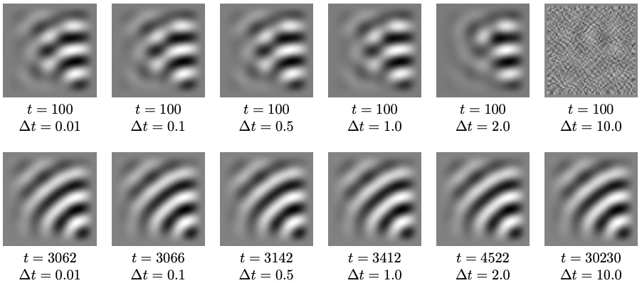
Figure 2: Pattern developed with the SH3 model, GDBC, forced with a spatial ramp of the control parameter given by $0.0\leq\epsilon(\mathbf{x})\leq 0.2$, and six different time steps. Top row: transient states at $t=100$. Bottom: the steady state for the six time steps. All tests started from the exactly same initial condition (pseudo-randomly generated) for a $64\times 64$ nodes domain. Note that the use of larger time steps results in smaller number of required steps to attain the same “time” ($t=100$ for instance). Errors with larger time steps result in delay in the emergence of the pattern and thus later steady states is expected.

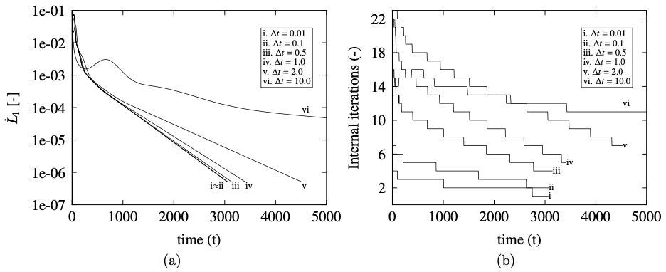
Figure 3: Scheme stability analysis from the numerical integration of the Swift-Hohenberg equation. (a) $\dot{L}_{1}$ and (b) internal iterations are shown as a function of time $t$ for a $64\times 64$ nodes domain for all six tests are presented in Fig. 2. The same steady pattern is reached for all six analyzed cases independently of the time step. The simulations started from the same random initial conditions.

Since the semi-implicit scheme is unconditionally stable for any time step, the CPU time to reaching the desired numerical solutions can be be optimized without major restrictions to selected time step, as shown by Table 2. A conservative choice for all simulations would be $\Delta t=0.1$, which presents the same $\dot{L}_{1}$ decay curve as for $\Delta t=0.01$. The choice for the remainder of this work was $\Delta t=0.5$ for the SH3 simulations and $\Delta t=0.1$ for the SH35, so that lower computational time is required without losing physically consistent transient results given the numerical scheme stability.

Table 2: Computational time spent on each of the simulations presented in 2. simulations.

Time	Minimum	Maximum	Steady	Computational
step	iterations	iterations	state	time spent
$\Delta t=0.01$	1	23	$t=3062$	234.4
$\Delta t=0.1$	2	15	$t=3066$	6.6
$\Delta t=0.5$	4	18	$t=3142$	1.7
$\Delta t=1.0$	5	22	$t=3412$	1.4
$\Delta t=2.0$	7	23	$t=4522$	1.2
$\Delta t=10.0$	7	16	$t=30230$	1

3.2 Convergence analysis

The adopted method to verify the order of accuracy of the code is the method of manufactured solutions (MMS). It provides a convenient way of verifying the implementation of nonlinear numerical algorithms by using a manufactured (artificial) solution for such purpose [37, 38, 36]. In terms of the proposed problem, we take all the members of the SH equation (3) and consider the following differential equation:

$$G\left(\psi\right)\;=\;0,$$ (22)

where $\psi$ is the order parameter function that satisfies Eq. (22) and therefore is the PDE solution. The MMS consists of adopting an arbitrary function to be the manufactured solution, $\psi_{m}(\mathbf{x},t)$, and since this function is not likely to solve the PDE, a source term is expected, $s_{m}$. This term can be seen as an additional forcing function, leading to a modified operator with this new source:

$$\bar{G}\left(\psi\right)\equiv G\left(\psi\right)-s_{m}.$$ (23)

For the previous equation, $\bar{G}\left(\psi_{m}\right)=0$ and $\bar{G}\left(\psi\right)=-s_{m}$. Following this new approach to the problem, we find an approximate numerical solution, $\psi_{k}$, for the discretized problem so that $\bar{G}\left(\psi_{k}\right)=0$ or $G\left(\psi_{k}\right)=s_{m}$. This source term is a minimal intrusion to the code’s formulation. The chosen function is periodic with a wavenumber $q_{1}$ and is defined as:

$$\psi_{m}(\mathbf{x},t)\;=\;\psi_{0}+\psi_{xy}\cos[q_{1}(x+y)]e^{at},$$ (24)

where all parameters employed in the manufactured solution and in the differential equation are present on Table 3.

Table 3: Parameters assumed for the manufactured solution adopted in the convergence analysis.

MS Parameters	Value	SH Parameters	Value
$q_{1}$	$0.25\sqrt{2}q_{0}$	$\epsilon$	-0.1
$q_{1}^{*}$	$\sqrt{2}q_{0}$	$q_{0}$	1.0
$\psi_{0}$	0.0	$\alpha$	1.0
$\psi_{xy}$	$\sqrt{|\epsilon|}$	$\beta$	-1.0
$a$	0.0	$\gamma$	0.0

The global discretization error was examined by the $L_{2}$ norm, defined as follows:

$$L_{2}\;=\;\left(\frac{\sum\limits_{i=1}^{n_{x}}\sum\limits_{j=1}^{n_{y}}\mid(\psi_{k})_{i,j}^{n}-(\psi_{m})_{i,j}^{n}\mid^{2}}{\sum\limits_{i=1}^{n_{x}}\sum\limits_{j=1}^{n_{y}}\mid(\psi_{m})_{i,j}^{n}\mid^{2}}\right)^{1/2}.$$ (25)

In the previous section, a second-order scheme was presented and therefore the formal order of accuracy is two. The observed order of accuracy of the code can be acquired from the global discretization error for meshes with different grid spacing, and can described by the following relation:

$$p\;=\;\dfrac{\ln\left({L_{2}^{B}}/{L_{2}^{A}}\right)}{\ln(r)},$$ (26)

where $L_{2}^{A}$ and $L_{2}^{B}$ are the $L_{2}$ norm for meshes A and B respectively, and $r$ is the ratio of the grid resolution $g_{r}$, given in number of mesh nodes per critical wavelength of mesh B to A. The meshes employed for the present tests, the number of nodes, and grid resolutions are shown in Table 4, and the $L_{2}$ curves for the numerical experiments can be seen in Fig. 4.

Table 4: Meshes employed for the code verification by MMS. The chosen domain for the test has $4\times 4$ critical wavelengths. The observed order of accuracy of the code in Fig. 4 can be calculated using Eq. (26) for two cases: $q_{1}=0.25\sqrt{2}q_{0}$ and $q_{1}^{*}=\sqrt{2}q_{0}$. In the first case the formal order of accuracy is achieved, $p\approx 2.0$, while in the second case $p^{*}\approx 4.0$ due to discretization error canceling.

Mesh	Number	Grid	Convergence rate ($p$)
	of nodes	resolution ($g_{r}$)	$\left(q_{1}=0.25\sqrt{2}q_{0}\right)$	$\left(q_{1}^{*}=\sqrt{2}q_{0}\right)$
Mesh A	$16\times 16$	4	-	-
Mesh B	$32\times 32$	8	$1.99514004$	$3.95294357$
Mesh C	$64\times 64$	16	$1.99862314$	$3.98876043$
Mesh D	$128\times 128$	32	$1.99964767$	$3.99722721$
Mesh E	$256\times 256$	64	$1.99991139$	$3.99916624$

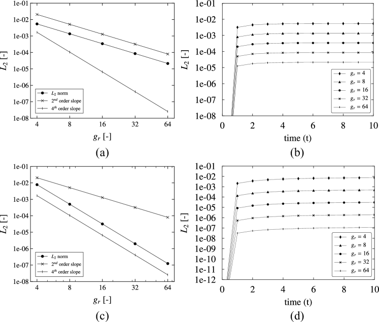
Figure 4: The observed order of accuracy of the code using Eq. (26) for both cases shown in Table 4. In first case, the $L_{2}$ norm is parallel to the (a) second-order slope and in the second case it is parallel to the (c) fourth-order slope. The resulting curves for the $L_{2}$ norm evolution in time are shown for the (b) first and (d) second case. Both $L_{2}$ norm evolutions start from values close to the machine precision ($10^{-16}$), since we start the convergence analysis simulations from the exact solution. In the first case the formal order of accuracy is achieved, $p\approx 2.0$, while in the second case $p^{*}\approx 4.0$ due to discretization error canceling.

A truncation error canceling could be seen when the choice for the manufactured solution wavenumber was $q_{1}=\sqrt{2}q_{0}$. The latter modifies the expected convergence rate up to fourth-order, which is consistent with the analytical development of the manufactured solution in Eq. (23). To verify the general case, we construct a manufactured solution with $q_{1}\neq\sqrt{2}q_{0}$. Following this approach, a second-order convergence rate is recovered as theoretically expected.

The numerical scheme has been proven to be consistent, unconditionally stable and truly second-order accurate in space, in the general case. The chosen grid resolution for the numerical experiments, presented in the next section, was $g_{r}=16$, which has a good trade-off between resolution and computational cost in order to represent periodic solutions.

3.3 Lyapunov functional decay

The decay of the “free energy” (Lyapunov) functional is monitored so that we can confirm it is always monotonically decreasing until a minimum value is reached in the steady state. In order to take into account the assumed boundary conditions adopted in this work, we expand the bulk integrals to show that boundary integrals vanish, leading to a new expression for the free energy functional, which is discretized. Using integration by parts and the 2D Gauss theorem (first Green identity), we have:

$$\int_{\Omega}d\mathbf{x}\left(\psi\nabla^{2}\psi\right)=\oint_{\partial\Omega}\psi\dfrac{\partial\psi}{\partial n}dl-\int_{\Omega}d\mathbf{x}|\nabla\psi|^{2}\,,$$ (27)

where the first integral from the RHS vanishes for the assumed GDBC ($\psi=\partial\psi/\partial n=0\;\text{on}\;\partial\Omega$) and PBC (since “there are no boundaries”). Now Eq. (1) can be rewritten as:

$$\mathcal{F}[\psi]=\int_{\Omega}{d\mathbf{x}}\dfrac{1}{2}\left\{-{\epsilon(\mathbf{x})}\psi^{2}+{\alpha}\left[q_{0}^{4}\psi^{2}-2q_{0}^{2}(\nabla\psi)^{2}+(\nabla^{2}\psi)^{2}\right]-\dfrac{\beta}{2}\psi^{4}+\dfrac{\gamma}{3}\psi^{6}\right\}.$$ (28)

The Lyapunov functional associated to the SH equation is implemented through the discrete formula derived by Christov & Pontes (2001)[30] for the cubic version, and now extended for the quintic one. The formula presents a ${\cal O}\left(\Delta t^{2}+\Delta x^{2}+\Delta y^{2}\right)$ approximation of the functional given by Eq. (2). As pointed by those authors, the monotonic decay of the finite differences version is enforced, provided that the internal iterations converge.Observe that the rate of change of the functional for this choice of boundary conditions (GDBC and PBC) is given by

$$\dfrac{d\mathcal{F}}{dt}=\int_{\Omega}d\mathbf{x}\,\mu\dfrac{\partial\psi}{\partial t}=-\int_{\Omega}d\mathbf{x}\,|\mu|^{2}\leqslant 0\,,$$ (29)

which in time discrete form reads

$$\frac{{\cal F}^{n+1}-{\cal F}^{n}}{\Delta t}=\int_{\Omega}d\mathbf{x}\,\mu^{n+1/2}\left({\psi^{n+1}-\psi^{n}\over\Delta t}\right)+E_{r}\,,$$ (30)

such that the RHS is guaranteed to be always negative. To show the consistency of the scheme the error $E_{r}\propto\mathcal{O}(\Delta t^{\eta})$, for $\eta>0$. Hence, the gradient descent nature of the dynamical equation ensures that any consistent discretization must preseve the correspondent energy disspation property.

In other to show the latter, we input the RHS of the target scheme given by $\mu^{n+1/2}$ in Eq. (5) into Eq. (31):

$$E_{r}=\dfrac{1}{\Delta t}\left[{{\cal F}^{n+1}-{\cal F}^{n}}-\int_{\Omega}d\mathbf{x}\,\mu^{n+1/2}\left({\psi^{n+1}-\psi^{n}}\right)\right]\,,$$ (31)

$$\Delta tE_{r}= {\cal F}^{n+1}-{\cal F}^{n}-\int_{\Omega}d\mathbf{x}\,\dfrac{1}{2}\left[\epsilon(\mathbf{x})-\alpha\left(q_{0}^{2}+\nabla^{2}\right)^{2}+\beta\dfrac{\left(\psi^{n+1}\right)^{2}+\left(\psi^{n}\right)^{2}}{2}-\gamma\dfrac{\left(\psi^{n+1}\right)^{4}+\left(\psi^{n}\right)^{4}}{2}\right]\times$$

$$\left[({\psi^{n+1})^{2}-(\psi^{n})^{2}}\right]$$

$$=\, -\int_{\Omega}d\mathbf{x}\left[\,\frac{\gamma\left(\psi^{n+1}\right)^{6}}{12}-\frac{\gamma\left(\psi^{n+1}\right)^{4}\left(\psi^{n}\right)^{2}}{4}+\frac{\gamma\left(\psi^{n+1}\right)^{2}\left(\psi^{n}\right)^{4}}{4}-\frac{\gamma\left(\psi^{n}\right)^{6}}{12}\right.$$

$$\left.-\alpha q_{0}^{2}\psi^{n+1}\nabla^{2}\psi^{n}+aq_{0}^{2}\psi^{n}\nabla^{2}\psi^{n+1}-\frac{\alpha}{2}{\psi^{n+1}\nabla^{4}\psi^{n}}+\frac{\alpha}{2}{\psi^{n}\nabla^{4}\psi^{n+1}}\right]$$ (32)

Considering the GDBC and PBC, the divergent terms vanish (first Green identity) yielding the following error:

$$E_{r}=\,\Delta t^{2}\int_{\Omega}d\mathbf{x}\left[\gamma\frac{\left(\psi^{n+1}+\psi^{n}\right)^{3}}{12}\left(\mu^{n+1/2}\right)^{3}\right]$$ (33)

Therefore, we have shown that $E_{r}=O(\Delta t^{\eta})$, with $\eta=2$, and the discrete scheme is consistent, with second order accuracy.

Following Eq. (28), the discrete functional at each time step is given by:

$${\cal F}^{n}= \sum\limits_{i=1}^{n_{x}}\sum\limits_{j=1}^{n_{y}}\left[-{\epsilon\over 2}\left(\psi^{n}_{i,j}\right)^{2}-{\beta\over 4}\left(\psi^{n}_{i,j}\right)^{4}+{\gamma\over 6}\left(\psi^{n}_{i,j}\right)^{6}+{\alpha q_{0}^{4}\over 2}\left(\psi^{n}_{i,j}\right)^{2}\right]$$

$$-\frac{2\alpha q_{0}^{2}}{4}\sum\limits_{i=1}^{n_{x}}\sum\limits_{j=1}^{n_{y}} \left[{\psi^{n}_{i+1,j}-\psi^{n}_{i,j}\over\Delta x}\right]^{2}\!\!\!+\!\left[{\psi^{n}_{i,j}-\psi^{n}_{i-1,j}\over\Delta x}\right]^{2}\!\!\!+\!\left[{\psi^{n}_{i,j+1}-\psi^{n}_{i,j}\over\Delta y}\right]^{2}\!\!\!+\!\left[{\psi^{n}_{i,j}-\psi^{n}_{i,j-1}\over\Delta y}\right]^{2}$$

$$+\frac{\alpha}{2} \sum\limits_{i=1}^{n_{x}}\sum\limits_{j=1}^{n_{y}}\left[{\psi^{n}_{i+1,j}-2\psi^{n}_{i,j}+\psi^{n}_{i-1,j}\over\Delta x^{2}}+{\psi^{n}_{i,j+1}-2\psi^{n}_{i,j}+\psi^{n}_{i,j-1}\over\Delta y^{2}}\right]^{2}\,.$$ (34)

In order to verify that the numerical scheme is correctly implemented, we monitored the evolution of the Lyapunov functional (Eq. (34)) in all the performed simulations, and verified that the Lyapunov potential is always decreasing. As an example, we show two simulations with the cubic SH (with ramped $\epsilon$) and four with the quintic one (both uniformly and ramped $\epsilon$), and the evolution of the Lyapunov functional (Eq. (34)), of $\dot{L}_{1}$ and of the patterns observed through the order parameter $\psi(\mathbf{x},t)$. The patterns evolution and the associated $\dot{L}_{1}$ and Lyapunov potentials are presented in Figs. 5, 7, and 8. The simulations were run with ramps of the control parameter $\epsilon(\mathbf{x})$ along the $x$-direction for both GDBC and PBC. The two simulations with the SH3 model started from the same pseudo-random initial condition. The four simulations with the SH35 model started from a squared localized patch in the center of the cell. This pre-existing structure of stripes parallel to the $y$-direction were constructed by:

$$\psi(\mathbf{x},0)=A_{0}\cos(q_{0}x),$$ (35)

where $A_{0}=\left\{(\beta/(2\gamma))[1+\sqrt{1+\epsilon\gamma/\beta^{2}}]\right\}^{1/2}$, which is compatible with the expected field $\psi$ amplitude for a stable spatially homogeneous states, for the SH35 [12]. The results of these six simulations confirm the correct implementation of the numerical scheme for both equations, with a monotonic decay of the Lyapunov functional in all cases.

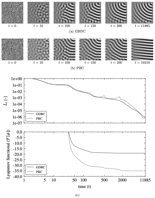
Figure 5: The results of two simulations run to verify the correctness of the implementation of the Lyapunov functional for the SH3 model. First and second rows: SH3 pattern evolution for a ramped system forced with $0.0\leq\epsilon\leq 0.2$ GDBC (a) and PBC (b), respectively, until the indicated steady state.. Both simulations started with the same pseudo-random initial condition. $\dot{L}_{1}$ and the Lyapunov potential evolutions are showed below.

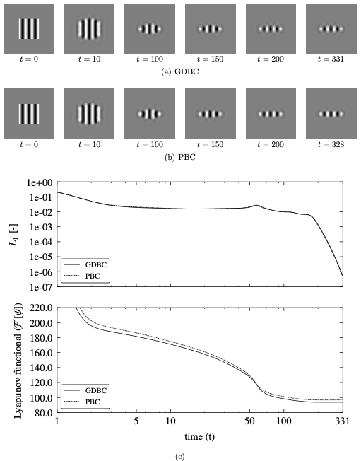
Figure 6: The results of two simulations run to verify the correctness of the implementation of the Lyapunov functional for the SH35 model. First and second rows: SH35 pattern evolution for a uniformly forced system with $\epsilon=-1.5$, GDBC (a) and PBC (b), respectively, until the indicated steady state.. Both simulations started from the same pre-existing structure of rolls perpendicular to the gradient of the control parameter. $\dot{L}_{1}$ and the Lyapunov potential evolutions are showed below.

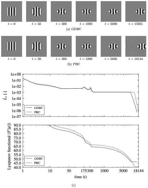
Figure 7: The results of two simulations run to verify the correctness of the implementation of the Lyapunov functional for the SH35 model. First and second rows: SH35 pattern evolution for a ramped system forced with $-1.5\leq\epsilon\leq-1.4$, GDBC (a) and PBC (b), respectively, until the indicated steady state.. Both simulations started from the same pre-existing structure of rolls perpendicular to the gradient of the control parameter. $\dot{L}_{1}$ and the Lyapunov potential evolutions are showed below.

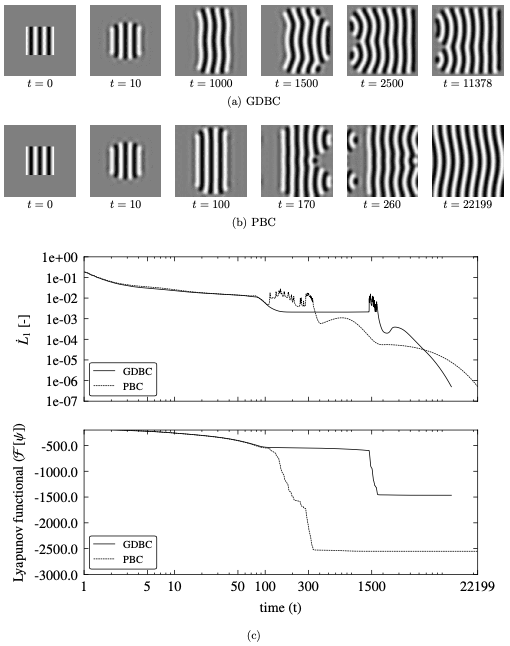
Figure 8: The results of two simulations run to verify the correctness of the implementation of the Lyapunov functional for the SH35 model. First and second rows: SH35 pattern evolution for a ramped system forced with $-1.4\leq\epsilon\leq-1.2$, GDBC (a) and PBC (b), respectively, until the indicated steady state.. Both simulations started from the same pre-existing structure of rolls perpendicular to the gradient of the control parameter. $\dot{L}_{1}$ and the Lyapunov potential evolutions are showed below.

4 Numerical experiments

The numerical scheme described in Sec. 2 is now used to solve the SH3 and the SH35 equations in square domains with rigid and periodic boundary conditions, and with nonuniform forcings. The adopted parameter values are given in Tables  1,  5 and 6. All simulations were done in a satisfactory grid resolution of the spatial grid of $16$ points per critical wavelength ($g_{r}=16$).

4.1 Numerical experiments with the SH3 equation

In the case of the SH3 equation we present the result of ten simulations (denoted as configurations $1$ to $10$), five of them with GDBC and five with PBC. The resulting steady states for each simulation are summarized in Fig. 9. All simulations started with the same pseudo-random initial condition. For each type of boundary condition we ran a configuration with uniform forcing to reproduce existing results, two configurations with ramps of the control parameter $\epsilon$, as detailed in Table 5, and two ones with different Gaussian distributions of the control parameter. In ramped systems, the parameter is assumed as uniform along the $y$-direction. The Gaussian distribution of $\epsilon$ introduces symmetric gradients in the radial direction.

The steady state solutions obtained are shown in Fig. 9. The first line in this figure shows the distribution of the control parameter $\epsilon$ along the $x$-direction of the domain. Second and fourth lines present the steady state solutions with rigid and with periodic boundary conditions, respectively. Third an fifth lines present the same results shown in lines two and four, but this time with frames constructed with enhanced contrast to make visible the subcritical structure developed in regions where the control parameter $\epsilon$ is negative. Each configuration run is identified with an assigned number.

Table 5: Parameters assumed for the numerical experiments with the SH3 equation.

Parameter		Formulæ		Value		Description
$q_{0}$		-		1.0		Critical wavenumber
$\lambda_{0}$		$2\pi/q_{0}$		$2\pi$		Critical wavelength
$w_{x}$, $w_{y}$		-		10		Wavelengths per domain length
$g_{r}$		-		16		Grid resolution (nodes per wavelength)
$n_{x}$, $n_{y}$		$w_{x}\times g_{r}$,$w_{y}\times g_{r}$		160		Nodes per mesh side ($n$)
$N$		$n_{x}\times n_{y}$		$160\times 160$		Total number of mesh nodes
$L_{x}$, $L_{y}$		$w_{x}\lambda_{0}$, $w_{y}\lambda_{0}$		$\approx 62.832$		Square domain length ($L$)
$\Delta x$,$\Delta y$		$L/(n-2)$		$\approx 0.3977$		Space step (GDBC)
$\Delta x$,$\Delta y$		$L/n$		$\approx 0.3927$		Space step (PBC)
$\Delta t$		-		0.5		Time step for SH3
$A$		-		0.2		Gaussian maximum value (peak)
$R_{1}$		$N$		-		For configurations 4 and 9
$R_{2}$		$0.2N$		-		For configurations 5 and 10
$x_{0}$,$y_{0}$		$L_{x}/2$,$L_{y}/2$		-		Gaussian center

Configuration 1 shows a pattern emerging in a uniformly forced system with GDBC, in qualitative agreement with previous results [23, 26, 27, 29]. This case was run for further verification of our numerical code. A pattern with unavoidable defects is developed, in order to match the strong requirement of rolls approaching perpendicularly the side walls. A structure with lower density of defects appears in configuration 6, where the same forcing of Frames 1 is assumed, but now, with periodic boundary conditions. The pattern develops a zig-zag instability.

Configuration 2 reproduces the result of a pattern developed in presence of a ramped control parameter $\epsilon$, with a subcritical region [28, 30, 29]. A structure with smaller amount of defects emerges, thanks to the fact that the weak structure of rolls parallel to the wall appears in the subcritical region. A similar situation occurs in configuration 3, where the system is forced with a ramp of the control parameter $\epsilon$ , however taking non negative values. In this case a weak structure of rolls perpendicular to the lower $(y=0)$ sidewall is visible.

Configurations 7 and 8 present the results for systems with same forcing of configurations 2 and 3, for the case of periodic boundary conditions. A tendency to develop a structure of rolls parallel to the gradient of the control parameter $\epsilon$ clearly appears, as well as the existence of a Benjamin-Feir instability close to the left wall, induced by the the supercritical region close to the right wall.

Configurations 4, 5, 9 and 10 present numerical results of simulations performed with a Gaussian radial distribution of the control parameter $\epsilon$, in the form:

$$\epsilon(\mathbf{x})=Ae^{-R((x-x_{0})^{2}+(y-y_{0})^{2})}\;,$$ (36)

where the parameters are specified in Table 5. The parameter $R$ is assumed to be $R_{1}$ in configurations 4 and 9; and $R_{2}$ in configurations 5 and 10. Worth noticing that these Gaussian distributions introduce a gradient of $\epsilon$ in all directions with the maximum of $\epsilon$ at the center of the domain.

Configurations 4 and 5 were run with rigid boundary conditions and configurations 9 and 10, with periodic conditions. A sharp Gaussian, rapidly decreasing from the maximum value across a short distance, leads to the onset of a target pattern with both boundary conditions. The target pattern collapses in presence of a wider Gaussian distribution of the control parameter $\epsilon$, leading to a structure of rolls. The structure wavevector takes the direction of one of the domain diagonals, again, since the most difficult direction for modulations of the structure is the one associated to the wavevector, whereas the easiest one is the direction perpendicular to the wavevector.

The time evolution of configurations 3 (GDBC) and 8 (PBC), from the pseudo-random initial condition to the steady state is shown in Fig. 10. The evolution of configurations 5 (GDBC) and 10 (PBC) are shown in Fig. 11. All curves reveal the expected result, with $\dot{L}_{1}$ rapidly decreasing as a pattern emerges and the amplitude of the structure essentially saturates. This stage is followed by a much slower phase dynamics, ending with an exponential decay towards the steady state. In general, $\dot{L}_{1}$ peaks are associated to the removal of defects. We observe that boundary conditions have little effect on the resulting curves.

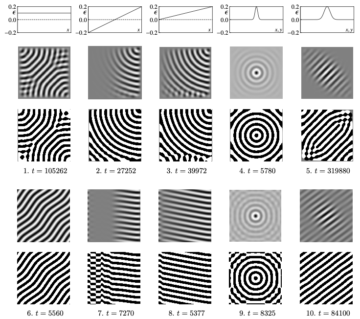
Figure 9: Zoology of ten patterns obtained by numerical integration of the SH3 equation with GDBC (rows 1 and 2) and PBC (rows 3 and 4). All patterns shown correspond to the steady attained when $\dot{L}_{1}\leq 5.0\times 10^{-7}$ (Eq. (21)). All simulations started from the same pseudo-random initial condition. The applied forcing is shown in the first row. First column: uniform forcing; Second and third columns: ramps of the control parameter $\epsilon$; Fifth and sixth columns: Two Gaussian forcings, according to Eq. (36). The first and third rows correspond to GDBC and PBC, respectively. Second and fourth rows contains the same patterns shown in rows one and three, respectively, with an enhanced contrast. Patterns configurations 2 and 3 tend to approach perpendicularly to the supercritical boundaries and parallel to subcritical ones. The pattern configuration 4 presents a target structure compatible with the narrow Gaussian profile of the forcing. The target collapses in the pattern configuration 5, and evolves to a structure of rolls parallel to one of diagonals, and not to the side walls. This effect occurs as a consequence of the modulation, which if harder along the direction of the pattern wavevector. Similar phenomena occurs with patterns configurations 9 and 10.

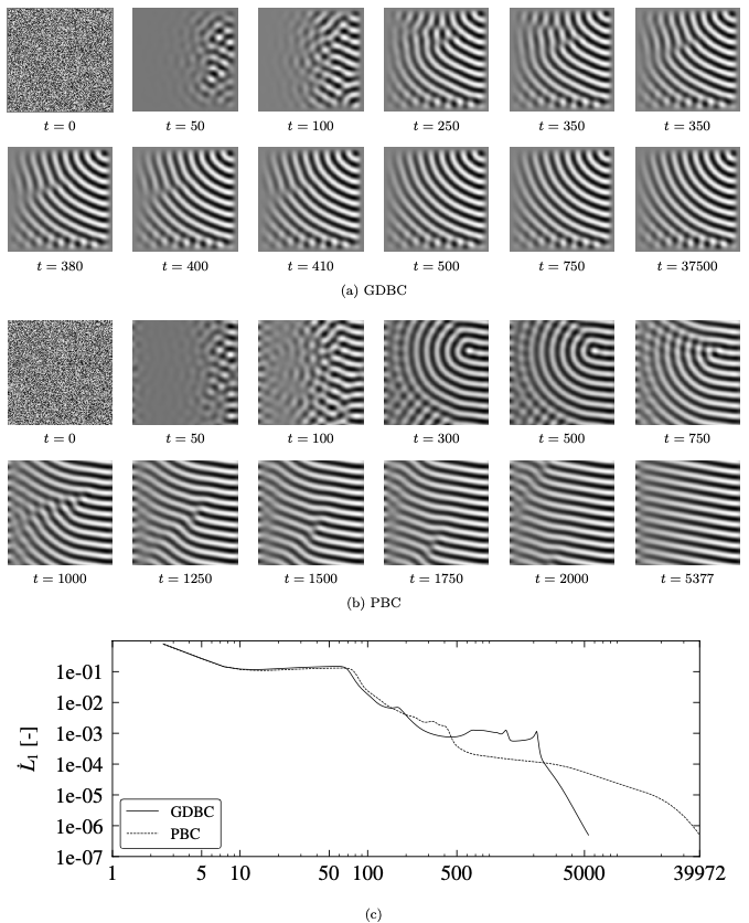
Figure 10: First and second lines: pattern evolution for the configuration 3 of Fig. 9, with GDBC (a), until the steady state. Third and fourth lines: pattern evolution for the configuration 8 of Fig. 9, with PBC (b), until the steady state. In both cases, the system is forced with a ramp of the control parameter $\epsilon$ along the $x$ direction, with $-0.2\leq\epsilon\leq 0.2$. The associated $\dot{L}_{1}\times t$ curves are also shown (c).

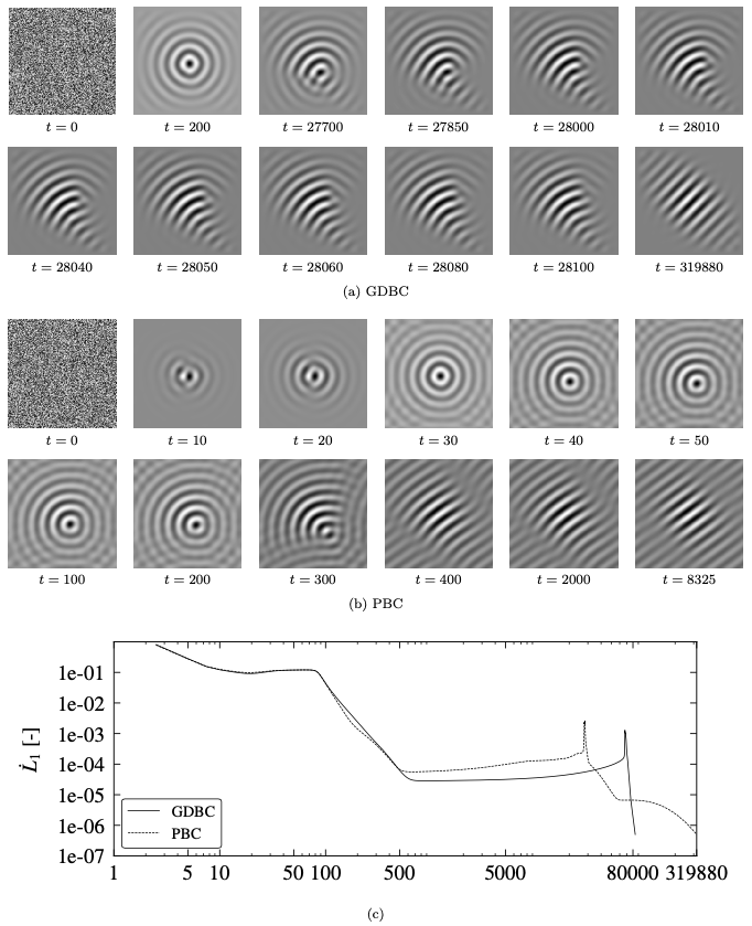
Figure 11: First and second lines: pattern evolution for the configuration 5 of Fig. 9, with GDBC (a), until the steady state. Third and fourth lines: pattern evolution for the configuration 10 of Fig. 9, with PBC (b), until the steady state. In both cases, the system is forced with a Gaussian distribution of the control parameter $\epsilon$. The associated $\dot{L}_{1}\times t$ curves are also shown (c).

4.2 Numerical experiments with the SH35 equation

The quintic version of the Swift-Hohenberg equation with destabilizing cubic term allows for the existence of stable localized solutions for an interval of subcritical values of $\epsilon$, i.e. coexistence of the solution $\psi=0$ and a modulated one, shown by  [12]. The parameter values adopted are given in Table 6. In this sense, we run six experiments with the SH35 equation: two with uniform forcing $(\epsilon=-1.5)$, GDBC and PBC, respectively, two with a ramp $-1.5\leq\epsilon\leq-1.4$, GDBC and PBC, respectively, and two last ones with a ramp $-1.4\leq\epsilon\leq-1.2$, GDBC and PBC, respectively. The experiments with uniform forcing were conducted as code verification, to reproduce existing results. The time evolution of these two experiments are shown in Fig. 6. Both simulations started from the same pseudo-random initial condition.

The four experiments with ramped systems started from the same pre-existing structure of rolls perpendicular to the gradient of the control parameter. These experiments were used to verify the implementation of the Lyapunov functional with the quintic equation SH35. The evolution of these simulations are shown in Fig. 7, and 8. In the case of a ramp given by $-1.5\leq\epsilon\leq-1.4$ the pre-existing structure evolves towards a localized structure of rolls with the same orientation of the initial condition, with both boundary conditions. When the applied forcing takes the form $-1.4\leq\epsilon\leq-1.2$, lowering the energy associated with the non-trivial solution both with GDBC and PBC, a structure of rolls with the same orientation of the initial condition also prevails, but the final structure is localized with GDBC and occupies the entire domain, with PBC.

Table 6: Parameters assumed for the numerical experiments with the SH35 equation.

Parameter		Formulæ		Value		Description
$q_{0}$		-		1.0		Critical wavenumber
$\lambda_{0}$		$2\pi/q_{0}$		$2\pi$		Critical wavelength
$w_{x}$, $w_{y}$		-		8		Wavelengths per domain length
$g_{r}$		-		16		Grid resolution (nodes per wavelength)
$n_{x}$, $n_{y}$		$w_{x}\times g_{r}$,$w_{y}\times g_{r}$		128		Nodes per mesh side ($n$)
$N$		$n_{x}\times n_{y}$		$128\times 128$		Total number of mesh nodes
$L_{x}$, $L_{y}$		$w_{x}\lambda_{0}$, $w_{y}\lambda_{0}$		$\approx 50.266$		Square domain length ($L$)
$\Delta x$,$\Delta y$		$L/(n-2)$		$\approx 0.3989$		Space step (GDBC)
$\Delta x$,$\Delta y$		$L/n$		$\approx 0.3927$		Space step (PBC)
$\Delta t$		-		0.1		Time step for SH35

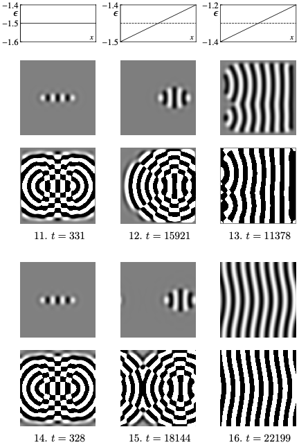
Figure 12: Zoology of six patterns obtained by numerical integration of the SH35 equation with GDBC (rows 1 and 2) and PBC (rows 3 and 4). All patterns shown correspond to the steady attained when $\dot{L}_{1}\leq 5.0\times 10^{-7}$ (Eq. (21)) All simulations started from a pre-existing structure of stripes oriented along the $y$ direction. The applied forcing is shown in the first row. First column: uniform forcing with $\epsilon=-1.5$. Second column: forcing with ramp of the control parameter in the form $-1.5\leq\epsilon\leq-1.4$. Third column: ramp in the form $-1.4\leq\epsilon\leq-1.2$. The first and third rows correspond to GDBC and PBC, respectively. Second and fourth rows contain the same patterns shown in rows one and three, respectively, with an enhanced contrast. In all cases, the pre-existing structure of stripes oriented along the $y$ prevails at the steady state. However, configurations 11, 12, 14 and 15 evolved to localized structures, whereas, in the case of configurations 13 and 16 the resulting pattern occupy the entire domain.

4.3 Discussion

We extended a numerical scheme proposed by Christov & Pontes [29] to investigate pattern formation modelled by the cubic SH equation in two dimensions.

Our work includes the quintic SH equation and PBC for both the cubic and the quintic SH, with a scheme that retains all characteristics of the original one: strict representation of the Lyapunov functional, unconditional stability, and second order representation of all derivatives. We additionally implement different nonuniform forcing field, such as ramps and Gaussian distributions. A detailed study of the effects of nonuniform forcings are addressed in a paper that builds on the present numerical scheme [39].

Verification tests consisted in qualitatively reproducing existing results of SH3 and SH35 simulations with uniform forcings for both GDBC and PBC, where good agreement was observed. As an additional verification procedure, we also found good agreement between the results obtained from the SH3 forced with a spatial ramp of $\epsilon$, and those presented by Pontes et al. (2008)[29]. In that work, the authors adopted GDBC and a first order approximation in time. The results of the SH3 equation with GDBC and ramps of $\epsilon$ are presented in Figs. 2, 5a and in simulations configurations 1, 2 and 3 of Fig. 12.

Rigid boundary conditions (GDBC) make patterns of supercritical stripes developed close to different boundaries to compete, due to the tendency of stripes to approach boundaries perpendicularly to them. That is, stripes cannot be perpendicular to all boundaries simultaneously. In addition, boundary effects compete with bulk ones. The overall result is a structures with high density of defects. A different situation occurs when PBC are imposed. In this case, a periodicity is imposed to the emerging pattern, and boundary effects are excluded. The result is, in general, a pattern with fewer defects than ones developed with the same forcing and GDBC. This is also the case when the system is forced with nonuniform distributions of the control parameter.

An important configuration in nonuniformly forced systems consists in adopting GDBC, and a forcing where part of the domain is maintained at subcritical conditions. In this case a less known result points to the fact that the subcritical pattern of stripes, induced by the supercritical region, approach sidewalls parallel to them. These patterns are automatically perpendicular to adjacent walls. As a result, nonuniformly forced systems with a subcritical region tend to develop patterns with a lower density of defects than systems uniformly forced [29]. The presented simulations reproduce this effect.

A particular feature observed in nonuniformly forced systems, using the SH3 equation, PBC and spatial ramps of the control parameter, consists in the development of several examples of the Benjamin-Feir instability, which manifest itself in the form of “alternating” rolls, in a dislocation sense, promoted by a region where minimum and maximum values of $\epsilon$ are close.

The quintic SH35 equation with a destabilizing cubic term allows for the emergence of localized solutions in an interval of subcritical values of $\epsilon$. Six simulations were run with the quintic equation, assuming three different forcings and two boundary conditions for each one. All simulations started from the same pseudo-random initial condition. The resulting steady states are presented in Fig. 12. The first group consisted of two simulations with uniform forcing $\epsilon=-1.5$. These simulations are denoted by configurations 11 and 14 in Fig. 12 The second group was forced with a ramp along the $x$ direction, given by $-1.5\leq\epsilon\leq-1.4$ (configurations 12 and 15). The third group was run with $-1.4\leq\epsilon\leq-1.2$ (configurations 13 and 16). In all configurations, the resulting patterns consisted of stripes perpendicular to the gradient of the control parameter, with localized patterns in the first and second groups, and the stripes occupying the entire domain in the third group. A mesh of $g_{r}=16$ points per critical wavelength was adopted in all simulations, which represents a good trade-off between spatial resolution and computational cost.

The uniqueness of the numerical solutions of the SH equation has not been proved. We note that both the explicit terms, and the operators allocated to the implicit ones contain nonlinear terms. The scheme preserves both the intrinsic ability of nonlinear dynamics of generating new modes, and the sensitivity to the prescribed initial condition. Due to that, minor changes in the initial condition may change the final patterns. However, this property is restricted by geometric, bulk, boundary effects, reducing the possible steady states. Bulk effects include the level of forcing, gradients of the control parameter and imposed periodicity. For instance we can expect that the patterns developed in configurations 1 to 5 of Fig. 9 could be mirror images with respect to the lower horizontal boundary, but not much more. The level of forcing is low and boundary effects prevail. The number of possible solutions is strongly reduced. At higher forcings small changes in the initial conditions may result in patterns with quantitatively different distribution of defects. The number of solutions is larger. In addition, some solutions may exist but are unstable, and not observed. This is the case of structures containing more than one mode at each point, which lead to structures of rhombs, and hexagons.

5 Conclusion

In this article, we extended a numerical scheme proposed by Christov & Pontes [29] to investigate pattern formation modeled by the cubic Swift-Hohenberg equation in two dimensions. The original scheme presents second order representation of all derivatives, strict implementation of the associated Lyapunov functional, rigid boundary conditions, and a semi-implicit assignment of the terms. The present work includes the quintic version of the Swift-Hohenberg equation and periodic boundary conditions for both the cubic and the quintic versions of the model. The scheme retains all characteristics of the original one, namely strict representation of the Lyapunov functional, unconditional stability, and second order representation of all derivatives. In addition, we also included a convergence analysis, new verification tests, and an initial evaluation of the effect of nonuniform forcings in the form of spatial ramps and of Gaussian distributions of the control parameter $\epsilon$. Among the verification tests, the convergence analysis confirmed the truly second-order accuracy of the scheme both in space and time and the existence of localized structures developed in the framework of the quintic equation even with nonuniform forcings. The conducted tests confirmed the robustness of the developed tool for pursuing the investigation of the pattern formation through the parabolic Swift-Hohenberg equation presenting various nonlinear terms, including nonuniform forcings.

Additionally, the numerical experiments conducted in this work suggest the existence of effects and the onset of patterns not addressed in the literature. Both questions are the object of a companion study [39], based on the present numerical framework.

6 Acknowledgments

The authors thank FAPERJ (Research Support Foundation of the State of Rio de Janeiro) and CNPq (National Council for Scientific and Technological Development) for the financial support. Daniel Coelho acknowledges a fellowship from the Coordination for the Improvement of Higher Education Personnel-CAPES (Brazil). A FAPERJ Senior Researcher Fellowship is acknowledged by J. Pontes. The authors dedicate a special posthumous thanks to C. I. Christov, who performed great development regarding the numerical methods addressed in this paper.

References

- Yang et al. [2004] L. Yang, A. M. Zhabotinsky, I. R. Epstein, Stable squares and other oscillatory turing patterns in a reaction-diffusion model, Physical review letters 92 (2004) 198303.
- Moloney and Newell [2008] J. V. Moloney, A. C. Newell, Nonlinear Optics, Westview Press, 2008.
- Walgraef [1997] D. Walgraef, Spatio-Temporal Pattern Formation: With Examples from Physics, Chemistry, and Materials Science, Partially Ordered Systems, 1 ed., Springer-Verlag New York, 1997.
- Ghoniem and Walgraef [2008] N. Ghoniem, D. Walgraef, Instabilities and Self-organization in Materials, Oxford Univ. Press, 2008.
- Provatas and Elder [2010] N. Provatas, K. Elder, Phase-Field Methods in Materials Science and Engineering, Wiley, 2010.
- Plapp and Karma [2000] M. Plapp, A. Karma, Multiscale finite-difference-diffusion-monte-carlo method for simulating dendritic solidification, Journal of Computational Physics 165 (2000) 592–619.
- Provatas et al. [2005] N. Provatas, M. Greenwood, B. Athreya, N. Goldenfeld, J. Dantzig, Multiscale modeling of solidification: phase-field methods to adaptive mesh refinement, International Journal of Modern Physics B 19 (2005) 4525–4565.
- Ghosh and Plapp [2017] S. Ghosh, M. Plapp, Influence of interphase boundary anisotropy on bulk eutectic solidification microstructures, Acta Materialia 140 (2017) 140–148.
- Ghosh et al. [2019] S. Ghosh, A. Karma, M. Plapp, S. Akamatsu, S. Bottin-Rousseau, G. Faivre, Influence of morphological instability on grain boundary trajectory during directional solidification, Acta Materialia 175 (2019) 214–221.
- Swift and Hohenberg [1977] J. Swift, P. C. Hohenberg, Hydrodynamic fluctuations at the convective instability, Physical Review A 15 (1977).
- Pontes et al. [2006] J. Pontes, D. Walgraef, E. Aifantis, On dislocation patterning: Multiple slip effects in the rate equation approach, International journal of plasticity 22 (2006) 1486–1505.
- Sakaguchi and Brand [1996] H. Sakaguchi, H. R. Brand, Stable localized solutions of arbitrary length for the quintic Swift-Hohenberg equation, Physica D 97 (1996) 274–285.
- Avitabile et al. [2010] D. Avitabile, D. J. Lloyd, J. Burke, E. Knobloch, B. Sandstede, To snake or not to snake in the planar Swift–Hohenberg equation, SIAM Journal on Applied Dynamical Systems 9 (2010) 704–733.
- Walton [1982] I. Walton, On the onset of Rayleigh-Bénard convection in a fluid layer of slowly increasing depth, Studies in Applied Mathematics 67 (1982) 199–216.
- Walton [1983] I. Walton, The onset of cellular convection in a shallow two-dimensional container of fluid heated non-uniformly from below, Journal of Fluid Mechanics 131 (1983) 455–470.
- Elder et al. [2002] K. Elder, M. Katakowski, M. Haataja, M. Grant, Modeling elasticity in crystal growth, Physical review letters 88 (2002) 245701.
- Elder and Grant [2004] K. Elder, M. Grant, Modeling elastic and plastic deformations in nonequilibrium processing using phase field crystals, Physical Review E 70 (2004) 051605.
- Langer and Müller-Krumbhaar [1978] J. Langer, H. Müller-Krumbhaar, Theory of dendritic growth—i. elements of a stability analysis, Acta Metallurgica 26 (1978) 1681–1687.
- Langer [1980] J. S. Langer, Instabilities and pattern formation in crystal growth, Reviews of modern physics 52 (1980) 1.
- Elsey and Wirth [2013] M. Elsey, B. Wirth, A simple and efficient scheme for phase field crystal simulation, ESAIM: Mathematical Modelling and Numerical Analysis 47 (2013) 1413–1432.
- Lee and Kim [2016] H. G. Lee, J. Kim, A simple and efficient finite difference method for the phase-field crystal equation on curved surfaces, Computer Methods in Applied Mechanics and Engineering 307 (2016) 32–43.
- Li and Kim [2017] Y. Li, J. Kim, An efficient and stable compact fourth-order finite difference scheme for the phase field crystal equation, Computer Methods in Applied Mechanics and Engineering 319 (2017) 194–216.
- Greenside and W. M. Coughran [1984] H. S. Greenside, J. W. M. Coughran, Nonlinear pattern formation near the onset of Rayleigh-Bénard convection, Physical Review A 30 (1984) 398–428.
- Cross [1982a] M. Cross, Ingredients of a theory of convective textures close to onset, Physical Review A 25 (1982a) 1065.
- Cross [1982b] M. Cross, Boundary conditions on the envelope function of convective rolls close to onset, The Physics of Fluids 25 (1982b) 936–941.
- Manneville [1990] P. Manneville, Non-equilibrium Structures and Weak Turbulence, Academic Press: San Diego, CA, USA, 1990.
- Cross [1983] M. C. Cross, Pattern formation outside equilibrium, Rev. Modern Physics 65 (1983) 851–1112.
- Christov et al. [1997] C. Christov, J. Pontes, D. Walgraef, M. Velarde, Implicit time splitting for fourth-order parabolic equations, Computer Methods in Applied Mechanics and Engineering 148 (1997).
- Pontes et al. [2008] J. Pontes, D. Walgraef, C. I. Christov, Pattern formation in spatially ramped Rayleigh-Bénard systems, Journal of Computational Interdisciplinary Sciences 1 (2008) 11–32.
- Christov and Pontes [2002] C. Christov, J. Pontes, Numerical scheme for Swift-Hohenberg equation with strict implementation of Lyapunov functional, Mathematical and Computer Modelling 35 (2002).
- Lee [2019] H. G. Lee, An energy stable method for the swift–hohenberg equation with quadratic–cubic nonlinearity, Computer Methods in Applied Mechanics and Engineering 343 (2019) 40–51.
- Vitral et al. [2019] E. Vitral, P. H. Leo, J. Viñals, Role of gaussian curvature on local equilibrium and dynamics of smectic-isotropic interfaces, Physical Review E 100 (2019) 032805.
- Wang and Zhai [2020] J. Wang, S. Zhai, A fast and efficient numerical algorithm for the nonlocal conservative Swift–Hohenberg equation, Mathematical Problems in Engineering (2020).
- Douglas and Rachford. [1956] J. Douglas, H. H. Rachford., On the numerical solution of heat conduction problems in two and three space variables, Trans. Amer. Math. Soc. (1956).
- Yanenko and Holt [1971] N. N. Yanenko, M. Holt, The Method of Fractional Steps, Springer, 1971.
- Vitral et al. [2018] E. Vitral, D. Walgraef, J. Pontes, G. Anjos, N. Mangiavacchi, Nano-patterning of surfaces by ion sputtering: Numerical study of the anisotropic damped Kuramoto-Sivashinsky equation, Computational Materials Science 146 (2018).
- Roache [2002] P. J. Roache, Code verification by the method of manufactured solutions, J. Fluids Eng. 124 (2002) 4–10.
- Roy [2005] C. J. Roy, Review of code and solution verification procedures for computational simulation, Journal of Computational Physics 205 (2005) 131–156.
- Coelho et al. [2021] D. L. Coelho, E. Vitral, J. Pontes, N. Mangiavacchi, Stripe patterns orientation resulting from nonuniform forcings and other competitive effects in the Swift–Hohenberg dynamics, Physica D: Nonlinear Phenomena 427 (2021) 133000.
- Podneks and Hamley [1996] V. E. Podneks, I. W. Hamley, Landau-Brazovskii theory for the structure, Journal of Experimental and Theoretical Physics Letters 64 (1996) 617–624.
- Boyer and Viñals [2002] D. Boyer, J. Viñals, Grain boundary pinning and glassy dynamics in stripe phases, Physical Review E 65 (2002).
- Marconi and Tarazona [2000] U. M. B. Marconi, P. Tarazona, Dynamic density functional theory of fluids, Journal of Physics: Condensed Matter 12 (2000) A413.