Bayesian Inversion for Anisotropic Hydraulic Phase-Field Fracture

Abstract

In this work, a Bayesian inversion framework for hydraulic phase-field transversely isotropic and orthotropy anisotropic fracture is proposed. Therein, three primary fields are pressure, displacements, and phase-field while direction-dependent responses are enforced (via penalty-like parameters). A new crack driving state function is introduced by avoiding the compressible part of anisotropic energy to be degraded. For the Bayesian inversion, we employ the delayed rejection adaptive Metropolis (DRAM) algorithm to identify the parameters. We adjust the algorithm to estimate parameters according to a hydraulic fracture observation, i.e., the maximum pressure. The focus is on uncertainties arising from different variables, including elasticity modulus, Biot’s coefficient, Biot’s modulus, dynamic fluid viscosity, and Griffith’s energy release rate in the case of the isotropic hydraulic fracture while in the anisotropic setting, we identify additional penalty-like parameters. Several numerical examples are employed to substantiate our algorithmic developments.

Keywords: Phase-field approach, hydraulic fracture, fluid-saturated porous media, anisotropic materials, Bayesian inference, DRAM algorithm.

1 Introduction

Hydraulic fracturing is a widely used technique to intentionally create fracture networks in rock materials by fluid injections. This process commonly used in low permeability rocks, for instance, shale structure and frequently used in the oil and gas industry [1]. Through fracking process water is injected with very high pressure in the well, to create intentionally a fracture network induced by pressure flow. The fracture network expands from natural cracks found in the vicinity of the well. Finally, the fracturing fluid is drained off [2].

Shale is one of the most abundant sedimentary rocks in the Earth’s crust and constitutes a large proportion of the clastic fill in sedimentary basins [3]. These types of rocks are known to be characterized by low porosity within the sedimentary rocks and also very low permeability [4]. Shale structures behave naturally in an anisotropic fashion [3] and therefore fracture responses highly depend on the interaction between structural properties of the material constituent [5]. Thus, the goal of the fracking process in the shale gas reservoir is to activate and open natural fractures and create an anisotropic fracture network [6].

In this work, fracture modeling is achieved with a phase-field method. The variational-based model to fracture by [7] and the related regularized formulation, commonly referred to a variational phase-field formulation [8, 9, 10] of brittle fracture is a widely accepted framework for fracture modeling. For strongly anisotropic fracture, e.g. shale structures, a higher-order phase-field framework with smooth local maximum entropy is proposed in [11] for crack propagation in brittle materials. In [12], a phase-field fracture setting for modeling anisotropic brittle material behavior under small and finite deformations was developed. The crack phase-field model was extended in [13] to include anisotropic fracture employing an anisotropic volume-specific fracture surface function. In [14], a modified phase-field model that can recognize between the critical energy release rates for mode I and mode II cracks was proposed for simulating mix-mode crack propagation in rock-like materials. A robust and efficient multiscale treatment (according to the Global-Local approach) was developed by the authors to model phase-field fracture in anisotropic heterogeneous materials [15].

Pressurized and fluid-filled fractures using phase-field modeling was subject in numerous papers in recent years. These studies range from mathematical modeling [16, 17, 18, 19, 20, 21, 22, 23], mathematical analysis [24, 25, 26, 27, 28], numerical modeling and simulations [29, 30, 31, 32, 33, 34, 35, 36, 37, 38, 39, 40], and up to (adaptive) global-local formulations [41] (see here in particular also [42] and [15] for non-pressurized studies) and high performance parallel computations [43, 44]. Extensions towards multiphysics phase-field fracture in porous media were proposed in which various phenomena couple as for instance proppant [23], two-phase flow formulations [45] or given temperature variations [20]. Recent reviews include [46] and [47].

In the previously described situations, uncertainties in parameters arise from several sources, e.g., heterogeneity of rock mass, variability in geologic formations, such as oil and gas reservoirs, formation and fluid properties, damage parameters, dynamic viscosity, or critical dissipation. Furthermore. material parameters fluctuate randomly in space. The mechanical material parameters (e.g., elasticity) are spatially variable and, hence, the uncertainty related to spatially varying properties can be represented by random fields. For instance, the material stiffness property has spatial variability. In order to provide a robust model, their uncertainty should be taken into consideration. Thus, the necessity of using an inverse approach (here we used the DRAM algorithm [48]) to estimate/identify the influential parameters, simultaneously, seems to be particularly demanding.

Bayesian inversion (as an inverse method) is a statistical technique to identify the various unknown parameters based on prior information (primary knowledge). The great advantage of the method is identifying the various parameters (at the same time) that they can no be measured straightly or only with significant experimental endeavors. We use the observations (i.e., experiment values or synthetic measurements [49]) to update the prior information, then obtain the posterior knowledge. Markov chain Monte Carlo (MCMC) is a common computational method to extract information according to an inverse problem. Metropolis-Hastings method is the most popular MCMC technique used by the authors for the first time in phase-field fracture [50]. Here, employing a reference value, i.e., load-displacement curve (estimated by a sufficiently fine mesh), the mechanical parameters (including Lamé constants and Griffith’s critical elastic energy release rate) identified precisely.

The main objectives of the underlying work are two-fold. First, a modular framework for a variational phase-field formulation of a hydraulic fracture toward anisotropic setting is formulated. We mainly extend the hydraulic phase-field fracture for the transversely isotropic poroelastic material and the layered orthotropic poroelastic materials. Here, direction-dependent responses due to the preferred fiber orientation in the poroelasticity material are enforced via additional anisotropic energy density function for both mechanical and phase-field equations. We derived a new consistent additive split for the bulk anisotropic energy density function to take into account only the tensile part of the energy. Thus, a modified crack driving state function is proposed such that it is only affected by the tensile part of both isotropic and also an anisotropic contribution, as well. Accordingly, a fully coupled monolithic approach for solving pressure and displacement is used while the computed results alternately fixed by solving the weak formulation corresponds to the crack phase-field. A detailed consistent linearization procedure with finite element discretization is further elaborated.

Second, in this work, a parameter estimation framework using Bayesian inversion for a hydraulic phase-field fracture of the isotropic/anisotropic setting is provided. Here, to enhance the performance of the MCMC method, we employ an adaptive Metropolis [51], delayed rejection [48] named DRAM. The method has been employed by the authors to estimate the effective physical and biological parameters in silicon nanowire sensors [52, 53]. Here, the main aim is to determine several effective parameters in the phase-field hydraulic fracture. For this, the maximum pressure during the fluid injection is chosen, and we strive to estimate the peak point and predict the crack behavior. The interested reader can refer to [54, 55] for the application of Bayesian inversion in porous media.

The outline of the paper is as follows. In Section 2, we present the mathematical framework and the variational phase-field model. The explain the model for isotropic materials and then derive a new setting to model hydraulic fractures in anisotropic materials. At the last step, as variational formulation will be derived for the coupled multi-field problem. We described how we used the finite element method to discretize the weak formulation and obtain the solutions, detailed in Appendix A. In Section 3, we present the DRAM algorithm and explain how it will be adjusted to identify the parameters in hydraulic fractures. In Section 4 four specific test experiments are given to verify the efficiency of the developed model, where the first two examples cover the isotropic materials. In the next numerical experiments, we consider the hydraulic fracture approach for transversely isotropic and orthotropy anisotropic fracture. Finally, the last section concludes the paper with some remarks.

2 Phase-field formulation of anisotropic hydraulic fracture

In this part, we model variational anisotropic phase-field fracture model toward poroelastic media, considering small deformations. Three governing equations are employed to characterize the constitutive formulations for the mechanical deformation, fluid pressure as well as the fracture phase-field. Afterward, we describe strong and variational formulations of the coupled multi-physics system. To formulate direction-dependent responses due to the preferred fiber orientation in the poroelasticity material, mechanical and phase-field equations are enforced via additional anisotropic energy density function.

2.1 Governing equations of poroelasticity

Let us consider $\mathcal{B}\in{\mathcal{R}}^{\delta}$ a solid in the Lagrangian (reference) configuration with dimension $\delta=2,3$ in the spacial direction, time $t\in\mathcal{T}=[0,T]$ and $\partial\mathcal{B}$ its surface boundary. Regarding the boundary condition, we assume Neumann conditions on $\partial_{N}\mathcal{B}\mathrel{\mathop{\mathchar 58\relax}}=\Gamma_{N}\cup\mathcal{C}$, where $\Gamma_{N}$ indicates the outer domain boundary and additionally Dirichlet boundary conditions on $\partial_{D}\mathcal{B}$.

The given boundary-value-problem (BVP) is a coupled multi-field system for the fluid-saturated porous media of the fracturing material. Fluid-saturated porous media can be formulated based on a coupled three-field system. At material points ${\mathbf{x}}\in\mathcal{B}$ and time $t\in\mathcal{T}$, the BVP solution indicates the displacement field ${\mathbf{u}}({\mathbf{x}},t)$ of the solid, the fluid pressure field $p({\mathbf{x}},t)$ as well as the crack which can be represented by

$${\mathbf{u}}\mathrel{\mathop{\mathchar 58\relax}}\left\{\begin{array}[]{ll}\mathcal{B}\times\mathcal{T}\rightarrow\mathcal{R}^{\delta}\\ ({\mathbf{x}},t)\mapsto{\mathbf{u}}({\mathbf{x}},t)\end{array}\right.,\quad\ p\mathrel{\mathop{\mathchar 58\relax}}\left\{\begin{array}[]{ll}\mathcal{B}\times\mathcal{T}\rightarrow\mathcal{R}\\ ({\mathbf{x}},t)\mapsto p({\mathbf{x}},t)\end{array}\right.,\quad\ d\mathrel{\mathop{\mathchar 58\relax}}\left\{\begin{array}[]{ll}\mathcal{B}\times\mathcal{T}\rightarrow[0,1]\\ ({\mathbf{x}},t)\mapsto d({\mathbf{x}},t)\end{array}.\right.$$ (1)

Considering $d({\mathbf{x}},t)=1$ in addition to $d({\mathbf{x}},t)=0$ are referred to the unfractured as well as completely fractured part of the material, respectively. Following Figure 1, the regularized fracture surface $\mathcal{C}_{l}$ is estimated in $\mathcal{B}_{L}\subset\mathcal{B}$ named fractured area. The unbroken area without fracture is defined as:

$$\mathcal{B}_{C}\mathrel{\mathop{\mathchar 58\relax}}=\mathcal{B}\backslash\mathcal{B}_{L}\subset\mathcal{B}\quad\text{such~{}that}\quad{\mathcal{B}}_{C}\cup{\mathcal{B}}_{L}=\mathrel{\mathop{\mathchar 58\relax}}\mathcal{B}~{}\text{and}~{}{\mathcal{B}_{C}}\cap{\mathcal{B}_{L}}=\varnothing.$$ (2)

For stating the variational formulations, we now introduce:

$$\bm{V}_{{\mathbf{u}}} \mathrel{\mathop{\mathchar 58\relax}}=\{{\bf H}^{1}(\mathcal{B})^{\delta}\mathrel{\mathop{\mathchar 58\relax}}\bm{u}=\bar{\bm{u}}\;\mathrm{on}\;\partial_{D}\mathcal{B}\},\quad$$ (3)

$$W \mathrel{\mathop{\mathchar 58\relax}}=\text{H}^{1}(\mathcal{B}),\quad W_{in}\mathrel{\mathop{\mathchar 58\relax}}=\{d\in\text{H}^{1}(\mathcal{B})^{\delta-1}|\;0\leq d\leq d^{old}\},$$

$${{V}_{p}} \mathrel{\mathop{\mathchar 58\relax}}=\{{H}^{1}(\mathcal{B})\mathrel{\mathop{\mathchar 58\relax}}p=\bar{p}\;\mathrm{on}\;\partial_{D}\mathcal{B}\}.$$

As typical in problems with inequality constraints (see e.g., [56, 57]), $W_{in}$ is a nonempty, closed, convex, subset of the linear function space $W$, which is no longer a linear space.

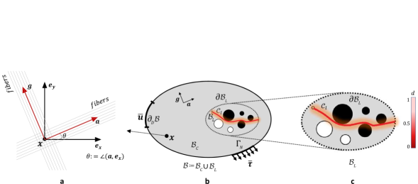
Figure 1: (a) Geometry and loading setup in a domain denoted by $\mathcal{B}$ whereas ${\mathcal{B}}_{C}$ stands for the unbroken domain, (b) zoom into the fractured region ${\mathcal{B}}_{L}\subset\mathcal{B}$ such that regularized ${\mathcal{C}}_{l}$ (the red curved crack surface) is approximated in this closed area, and (c) global Cartesian coordinate system with unit vectors $(\bm{e}_{\bm{x}},\bm{e}_{\bm{y}})$ and local orthogonal principal material coordinates corresponds to the first and second families of fibers $(\bm{a},\bm{g})$.

2.1.1 Mechanical contribution

Here, we represent the governing equations for brittle fracture in elastic solids at small strains. For isotropic materials, we can specify the energy stored in a bulk strain density the following constants

$$I_{1}(\bm{\varepsilon})=\text{tr}(\bm{\varepsilon}),\quad\quad I_{2}(\bm{\varepsilon})=\text{tr}(\bm{\varepsilon}^{2}).$$ (4)

Let the solid material is strengthened by two groups of fibers denoted as a orthotropic solid materials. Thus, an anisotropic material is reinforced by two fibers namely $\bm{a}$ and ${\mathbf{g}}$ with $\|\bm{a}\|=1$ and $\|{\mathbf{g}}\|=1$; see Figure 1. These materials have the highest strength in the fiber direction (i.e., either in $\bm{a}$ or $\bm{g}$). Therefore, at the material point $\bm{x}$, the stress state relates to the deformation in addition to the given direction which leads to a deformation-direction-dependent framework. For this, we impose a penalty-like parameter $\chi_{a}>0$ and $\chi_{g}>0$ corresponding to $\bm{a}$ or $\bm{g}$ which restrict a deformation on the normal plane to ${\mathbf{a}}$ or ${\mathbf{g}}$. Therefore, we can define three specific second-order tensorial quantities, i.e., the strain $\bm{\varepsilon}$ in addition to ${\mathbf{M}}$ and ${\mathbf{g}}$ tensors to specify the effective bulk free energy

$${\mathbf{\varepsilon}}=\nabla^{sym}{\mathbf{u}}=\text{sym}[\nabla{\mathbf{u}}],\quad{\mathbf{M}}\mathrel{\mathop{\mathchar 58\relax}}={\mathbf{a}}\otimes{\mathbf{a}},\quad\text{and}\quad{\mathbf{G}}\mathrel{\mathop{\mathchar 58\relax}}={\mathbf{g}}\otimes{\mathbf{g}}.$$ (5)

We employ two deformation-direction-dependent constants to clarify them as they can be represented by additional two

$$I_{4}=tr(\bm{\varepsilon\cdot M}),\quad I_{6}=tr(\bm{\varepsilon\cdot G}).$$ (6)

Considering the symmetric strain tensor $\bm{\varepsilon}$ and the structural tensors ${\mathbf{M}}$ and ${\mathbf{G}}$, we have the scalar-valued function ${\Psi}(\bm{\varepsilon};{\mathbf{M}},{\mathbf{G}})$. Therefore, the scalar-valued effective strain density function denotes an invariant in spatial and temporal directions between two sets of points in a specific domain under rotation. As a result, ${\Psi}(\bm{\varepsilon};{\mathbf{M}},{\mathbf{G}})$ is expressed by the seven principal invariants as

$${\Psi}(\bm{\varepsilon};{\mathbf{M}},{\mathbf{G}})={\Psi}\big{(}I_{1},I_{2},I_{4},I_{6}\big{)}=\widetilde{\Psi}^{iso}\big{(}I_{1},I_{2}\big{)}+\widetilde{\Psi}^{aniso}\big{(}I_{4},I_{6}\big{)}.$$ (7)

In this case, the isotropic free-energy function relates to

$$\widetilde{\Psi}^{iso}\big{(}I_{1},I_{2}\big{)}\mathrel{\mathop{\mathchar 58\relax}}=(\frac{K}{2})I^{2}_{1}-\mu~{}\Big{(}\frac{I^{2}_{1}}{\delta}-I_{2}\Big{)}\quad\text{with}\quad K>0\quad\text{and}\quad\mu>0,$$ (8)

where $K=\lambda+\frac{2}{3}\mu>0$ is the bulk modulus and including shear modulus $\mu$ with dimension in the spacial direction. Note, in our formulation, instead of using elastic Lamé’s first constant denoted by $\lambda>-\frac{2}{\mu}$ which has a lower bound, we used a shear bulk modulus as a positive quantity to avoid unnecessary condition. This has an advantage for our next goal; that is Bayesian estimation for the material parameters.

The anisotropic free-energy function can be specified by the anisotropic free-energy function for orthotropic materials reads

$$\widetilde{\Psi}^{aniso}\big{(}I_{4},I_{5},I_{6},I_{7}\big{)}\mathrel{\mathop{\mathchar 58\relax}}=\frac{1}{2}\chi_{a}I^{2}_{4}+\frac{1}{2}\chi_{g}I^{2}_{6}.$$ (9)

Again, $\chi_{a}$ and $\chi_{g}$ point out the anisotropic penalty-like material parameters.

To construct the mechanical BVP, let the geometry to be enforced by prescribed deformations $\overline{{\mathbf{u}}}$ and additionally the traction vector $\overline{\bm{\tau}}$ at the surface $\partial\mathcal{B}$ of the reference configuration, which are denoted by the time-dependent Dirichlet- and Neumann type boundary conditions as

$${\mathbf{u}}=\bar{\mathbf{u}}({\mathbf{x}},t)\ \textrm{on}\ \partial_{D}\mathcal{B}\quad\text{and}\quad{\bm{\sigma}}{\bm{\mathnormal{n}}}=\bar{}{\bm{\tau}}({\mathbf{x}},t)\ \textrm{on}\ \partial_{N}\mathcal{B}.$$ (10)

Here, ${\bm{\mathnormal{n}}}$ points out the unit normal vector in the reference setting such that the Cauchy stress tensor ${\bm{\sigma}}({\mathbf{\varepsilon}},p,d)$ denotes the thermodynamic dual to ${\mathbf{\varepsilon}}$. The global mechanical form of the equilibrium equation for the solid body can be represented through first-order PDE for the multi-field system as

$$\framebox{$\displaystyle\mbox{Div}\,{\bm{\sigma}}({\mathbf{u}},p,d)+\overline{\mathbf{b}}={\bm{\mathit{0}}}\,,$}$$ (11)

such that dynamic motion is neglected (i.e., quasi-static response), and we denote $\overline{\mathbf{b}}$ as a prescribed body force.

2.1.2 Fluid contribution

To formulate the constitutive equation for the poromechanics, let us move forward with a biphasic fully saturated porous material, which includes of pore fluid and a solid matrix within the bulk material. A local volume element denoted by $dV$ in the reference configuration is additively decomposed into a fluid portion $dV_{F}$ in addition to a solid portion $dV_{S}$. Thus, the volume fraction is introduced via $n_{c}\mathrel{\mathop{\mathchar 58\relax}}=dV_{c}/dV$, where $c=\{S,F\}$. Concerning the fully saturated porous medium the saturation condition reads

$$\sum_{c}n_{c}=n_{F}+n_{S}=1,$$ (12)

where $n_{F}({\mathbf{x}},t)$ indicates the porosity, which point out the volume occupied by the fluid is same as the pore volume. In the fracture zone we have

$$d=0\quad\mbox{leading to}\quad n_{S}=0\quad\mbox{also}\quad n_{F}=1.$$ (13)

The volume fraction in the porous medium, i.e., $n_{c}$, depends on the physical density (i.e., material, effective, intrinsic) $\rho_{cR}$ to the partial density $\rho_{c}$ through

$$\rho_{c}=n_{c}\;\rho_{cR}\quad\text{with}\quad\rho_{cR}\mathrel{\mathop{\mathchar 58\relax}}=dm_{c}/dV_{c}\quad\text{and}\quad\rho_{c}\mathrel{\mathop{\mathchar 58\relax}}=dm_{c}/dV,$$ (14)

where $dm_{c}$ denotes the mass of the phase $c$. Denoting the initial porosity $n_{F,0}$, for a constant fluid material density, the porosity (i.e., fluid volume fraction) $n_{F}$ is related to the fluid volume ratio $\theta$ (fluid content) per unit volume of the reference configuration $\mathcal{B}$ via

$$n_{F}=n_{F,0}+\theta,$$ (15)

where $\theta$ prescribes the first local internal variable (history field); see [58, 59, 60]. Also, the evolution equation for the fluid volume ratio $\dot{\theta}=\dot{n}_{F}$ can be obtained by means of the fluid pressure field $p$. Prescribed Dirichlet boundary condition and Neumann boundary condition for the pressure can be described by

$$p=\bar{p}({\mathbf{x}},t)\ \textrm{on}\ \partial_{D}\mathcal{B}~{}~{}~{}\text{and}~{}~{}~{}\bm{\mathcal{F}}\cdot{\bm{\mathnormal{n}}}=\bar{f}({\mathbf{x}},t)\ \textrm{on}\ \partial_{N}\mathcal{B},$$ (16)

through the fluid volume flux vector $\bm{\mathcal{F}}$, the imposed fluid pressure $\bar{p}$ on the boundary surface, fluid transport $\bar{f}$ on the Neumann boundary surface. Because the fluid-filled equation denotes a time-dependent problem, the initial condition needs to be set for the fluid volume rate and hence by $\theta({\mathbf{x}},t_{0})=0$ yielding $n_{F}=n_{F,0}$ in $\mathcal{B}$. Moreover, the fluid flux vector in (16) can be described through the negative direction of the material gradient of the fluid pressure $\nabla p$ through the permeability, based on Darcy-type fluid’s:

$$\bm{\mathcal{F}}\mathrel{\mathop{\mathchar 58\relax}}=-{\mathbf{K}}({\mathbf{\varepsilon}},d)\;\nabla p.$$ (17)

Here, the second-order permeability tensor is given by anisotropic second-order tensor ${\mathbf{K}}$ that described based on the strain tensor ${\mathbf{\varepsilon}}$ as well as the crack phase-field $d$. To denote the effect of the fracture on the fluid contribution, we decompose the permeability tensor into a Darcy-type flow for the unfractured porous medium $\bm{K}_{Darcy}$ in addition to a Poiseuille-type flow in a completely fractured material $\bm{K}_{crack}$ which is explained as follows

$$\begin{array}[]{ll}\bm{K}({\mathbf{\varepsilon}},d)&={\bm{K}_{Darcy}}({\mathbf{\varepsilon}})+(1-d)^{\zeta}{\bm{K}_{frac}}({\mathbf{\varepsilon}},d),\\[8.53581pt] {\bm{K}_{Darcy}}({\mathbf{\varepsilon}})&=K_{D}{\mathbf{I}},\\[8.53581pt] {\bm{K}_{frac}}({\mathbf{\varepsilon}},d)&=\big{(}\frac{\omega_{d}^{2}}{{12\eta_{F}}}-{{K}_{D}}\big{)}\;\;\big{[}{\mathbf{I}}-{\bm{\mathnormal{n}}}\otimes{\bm{\mathnormal{n}}}\big{]},\end{array}$$ (18)

with $\omega_{d}$ the so-called crack aperture (or the crack opening displacement) [61] defined as

$$\omega_{d}\mathrel{\mathop{\mathchar 58\relax}}=\llbracket{\mathbf{u}}({\mathbf{x}})\rrbracket.{\bm{\mathnormal{n}}}=({\bm{\mathnormal{n}}}\cdot{\mathbf{\varepsilon}}{\bm{\mathnormal{n}}})h_{e},$$ (19)

denoting the outward unit normal to the fracture surface ${\bm{\mathnormal{n}}}=\nabla d/|\nabla d|$ , ${K}_{D}$ in $\bm{K}_{Darcy}$ and $\bm{K}_{frac}$ indicates the isotropic intrinsic permeability of the pore space, $\eta_{F}$ represents the dynamic fluid viscosity, and $\zeta\geq 1$ denotes a permeability transition exponent. The characteristic element length $h_{e}$ in (19) typically set as a minimum discretized element size, i.e., diameter of an element in the fractured region; see [30]. Notably, the second-order permeability tensor in (18) in the intact region, i.e. $d=1$, recover ${\mathbf{K}}({\mathbf{\varepsilon}},d)\approx{{\mathbf{K}}_{Darcy}}({\mathbf{\varepsilon}})$. Following [30], The conservation of the fluid mass which reflects the second PDE within hydraulic fracturing setting reads

$$\dot{n}_{F}-\bar{r}_{F}+\mbox{Div}[\bm{\mathcal{F}}]=0\,,$$ (20)

by a given/imposed fluid source $\bar{r}_{F}$ per unit volume of the initial setting $\mathcal{B}$ describing the fluid injection process in the hydraulic fracturing.

2.1.3 Phase-field contribution

Within regularized fracture framework, a sharp-crack surface topology denoted by $\mathcal{C}$ to guarantee the continuity of the fracture field is further specified by the smeared fracture surface functional shown by $\mathcal{C}_{l}$ thus $\mathcal{C}\rightarrow\mathcal{C}_{l}$. Hence we have

$$\mathcal{C}_{l}(d)=\int_{\mathcal{B}}\gamma_{l}(d,\nabla d;{\mathbf{M}},{\mathbf{G}})\,dV\quad\text{with}\quad\gamma_{l}(d,\nabla d;{\mathbf{M}},{\mathbf{G}})\mathrel{\mathop{\mathchar 58\relax}}=\gamma^{iso}_{l}(d,\nabla d)+\gamma^{aniso}_{l}(\nabla d;{\mathbf{M}},{\mathbf{G}}),$$ (21)

where the isotropic part is

$$\gamma^{iso}_{l}(d,\nabla d)\mathrel{\mathop{\mathchar 58\relax}}=\frac{1}{2l}{(1-d)^{2}}+\frac{l}{2}\nabla d\cdot\nabla d,$$ (22)

and anisotropic part of phase-field density function reads

$$\gamma^{aniso}_{l}(\nabla d;{\mathbf{M}},{\mathbf{G}})\mathrel{\mathop{\mathchar 58\relax}}=\beta_{a}\frac{l}{2}\nabla d\cdot{\mathbf{M}}\cdot\nabla d+\beta_{g}\frac{l}{2}\nabla d\cdot{\mathbf{G}}\cdot\nabla d,$$ (23)

considering the anisotropic penalty-like material parameters $\beta_{a}$ and $\beta_{g}$. Here, $\gamma_{l}$ denotes the regularized crack surface density function per unit volume of the solid, the regularization item $l$ indicates the length scale (also named regularization parameter), which captures the fracture diffusivity. Therefore, we can derive $d$ (the crack phase-field) by minimizing diffusive crack surface $\mathcal{C}_{l}(d)$, as follows

$$d=\mbox{argmin}\{\inf_{d}\mathcal{C}_{l}(d)\}\quad\text{where}\quad d=0\;\mbox{on}\;\mathcal{C}\subset\mathcal{B}\;.$$ (24)

The outcome Euler-Lagrange differential system is

$$d-1-l^{2}\Delta d-\beta_{a}l^{2}\text{div}(\nabla d\cdot{\mathbf{M}})-\beta_{g}l^{2}\text{div}(\nabla d\cdot{\mathbf{G}})=0\quad in~{}\mathcal{B},$$ (25)

augmented by the homogeneous NBC that is $\nabla d\cdot{\bm{\mathnormal{n}}}=0$ on $\partial\mathcal{B}$. We then consider the smeared crack phase-field functional given in (21) to ensure the fracture Kuhn-Tucker conditions [20, 15]. To that end, the constitutive functions response by means of a global evolution system of regularized crack fracture gives rise to the global crack dissipation functional

$$\framebox{$\displaystyle\vphantom{\int_{\mathcal{B}}}\frac{d}{dt}\mathcal{C}_{l}(d)\mathrel{\mathop{\mathchar 58\relax}}=\frac{1}{l}\int_{\mathcal{B}}[\;-g^{\prime}(d_{+})\mathcal{H}+\eta\dot{d}\;]\;\dot{d}\,dV=\int_{\mathcal{B}}\;\delta\gamma_{l}(d,\nabla d;{\mathbf{M}},{\mathbf{G}})\dot{d}\,dV\geq 0\;,$}$$ (26)

results to the two inequity conditions for the crack phase-field through

$$\delta\gamma_{l}(d,\nabla d;{\mathbf{M}},{\mathbf{G}})\leq 0\quad\text{with}\quad\dot{d}\leq 0,$$ (27)

with the functional derivative of $\gamma_{l}$ with respect to $d$ by,

$$\int_{\mathcal{B}}\delta_{d}\gamma_{l}(d,\nabla d;{\mathbf{M}},{\mathbf{G}})\mathrm{d}{V}=\int_{\mathcal{B}}\frac{1}{l}[(d-1)-l^{2}\Delta d-\beta_{a}l^{2}\text{div}(\nabla d\cdot{\mathbf{M}})-\beta_{g}l^{2}\text{div}(\nabla d\cdot{\mathbf{G}})]\mathrm{d}{V}.$$ (28)

Additionally, in (26), $\mathcal{H}$ indicates the crack driving force and represent

$$\mathcal{H}=\max_{s\in[0,t]}D({\mathbf{x}},s)\geq 0,$$ (29)

where $D$ indicates the fracture driving state function. Furthermore, $\mathcal{H}$ considers the irreversibility of the crack phase-field evolution by filtering out a maximum value of $D$. This is referred to the local history variable. Also, an artificial/numerical material parameter (denoted by $\eta\geq 0$) is employed to specify the viscosity term of crack growth.

The local evolution of the crack phase-field equation in the given domain $\mathcal{B}$ resulting from (26) augmented with its homogeneous NBC, i.e. $\nabla d\cdot{\bm{\mathnormal{n}}}=0$ on $\partial\mathcal{B}$ yields

$$\framebox{$\displaystyle[\,d-1-l^{2}\Delta d-\beta_{a}l^{2}\text{div}(\nabla d\cdot{\mathbf{M}})-\beta_{g}l^{2}\text{div}(\nabla d\cdot{\mathbf{G}})\,]-\eta\dot{d}+2(1-\kappa)d{\mathcal{H}}=0\,,$}$$ (30)

which states the third equation in the coupled system.

2.2 Constitutive functions

The coupled BVP is formulated through three specific fields (i.e., unknown solution fields) to illustrate the hydro-poro-elasticity of fluid-saturated porous media in the fracturing material by

$$\mbox{Global Primary Fields}\mathrel{\mathop{\mathchar 58\relax}}{\Bgothic U}\mathrel{\mathop{\mathchar 58\relax}}=\{{\mathbf{u}},p,d\}.$$ (31)

Here, ${\mathbf{u}}$ is the displacement (mechanical deformation), $p$ denotes the pressure, and $d$ is the crack phase-field ($0\leq d\leq 1$). For the numerical implementation standpoint, to guarantee $0\leq d\leq 1$ holds, we project $d>1$ to 1 and $d<0$ to 0 to avoid unphysical crack phase-field solution [20]. The constitutive formulations for the hydraulic phase-field fracture are written in terms of the following set

$$\mbox{Constitutive State Variables}\mathrel{\mathop{\mathchar 58\relax}}{\Bgothic C}\mathrel{\mathop{\mathchar 58\relax}}=\{{\mathbf{\varepsilon}},\theta,d,\nabla d\}\ ,$$ (32)

which shows the response of the poroelasticity material modeling with a first-order gradient damage model. A pseudo-energy density function denoted by ${W}({\Bgothic C})$ for the poroelastic media per unit volume reads

$${W}({\Bgothic C})={W}_{elas}({\mathbf{\varepsilon}},d;{\mathbf{M}},{\mathbf{G}})+{W}_{fluid}({\mathbf{\varepsilon}},\theta)+{W}_{frac}(d,\nabla d;{\mathbf{M}},{\mathbf{G}}).$$ (33)

2.2.1 Fluid contribution

Following [62], the fluid density function takes the following form

$${W}_{fluid}({\mathbf{\varepsilon}},\theta)=\frac{M}{2}\Bigg{[}B^{2}tr^{2}[{\mathbf{\varepsilon}}]-2\,\theta\,tr[{\mathbf{\varepsilon}}]+\theta^{2}\Bigg{]}=\frac{M}{2}\big{(}B\;tr[{\mathbf{\varepsilon}}]-\theta\big{)}^{2},$$ (34)

based on the given fluid coefficient including which includes Biot’s coefficient $B$ and Biot’s modulus $M$. By employing the Coleman-Noll inequality condition in thermodynamics, the fluid pressure $p$ is derived from the first-order derivative of the pseudo-energy density function ${W}$ given in (33) by

$$p({\mathbf{\varepsilon}},\theta)\mathrel{\mathop{\mathchar 58\relax}}=\frac{\partial{W}}{\partial\theta}=\frac{\partial{{W}_{fluid}}}{\partial\theta}=\theta M-MBtr({\mathbf{\varepsilon}}),$$ (35)

for the isotropic solid material. Employing the above-mentioned pressure in addition to the second equation in (20) as well as (15), the conservation of mass takes the following form

$$\framebox{$\displaystyle\frac{\dot{p}}{M}+B~{}\partial_{t}{tr({\mathbf{\varepsilon}})}-\bar{r}_{F}+\mbox{Div}[\bm{\mathcal{F}}]=0,$}$$ (36)

which now depends on the fluid pressure $p$ and not fluid volume fraction (porosity).

2.2.2 Mechanical contribution

Here, modified elastic density function ${W}_{elas}$ is degraded elastic response resulting from the fractured state, a fluid density function contribution ${W}_{fluid}$, and fracture density function denoted by ${W}_{frac}$ which contain the accumulated dissipative energy are accordingly used. For a compressible isotropic elastic solid, the elastic density function is formulated through a linear elasticity strain energy function as

$${W}_{elas}({\mathbf{\varepsilon}},d;{\mathbf{M}},{\mathbf{G}})=g(d)\;{\Psi}({\mathbf{\varepsilon}};{\mathbf{M}},{\mathbf{G}}),$$ (37)

whereas $\Psi$ given in (7). Here, the standard monotonically decreasing quadrature degradation function, reads as $g(d)\mathrel{\mathop{\mathchar 58\relax}}=(1-\kappa)d^{2}+\kappa$.

2.2.3 Strain-energy decomposition for the bulk free energy

Since the fracturing materials behave significantly different in tension and compression, a consistent additive split for the strain energy density function given in (37) for the isotropic and anisotropic counterpart of energy are accordingly described. Thus, compared to other studies [13, 12, 15], we derived a new crack driving state function, which mainly includes the tensile part of anisotropic energy density function.

• Strain-energy decomposition for the isotropic term.

To derive an additive decomposition of the isotropic strain energy function, i.e. ${\Psi}^{iso}\big{(}I_{1}(\bm{\varepsilon}),$ $I_{2}(\bm{\varepsilon})\big{)}$, we carry out an additive split of the strain tensor $\bm{\varepsilon}(\bm{u})$ through

$$\bm{\varepsilon}(\bm{u})=\bm{\varepsilon}^{+}(\bm{u})+\bm{\varepsilon}^{-}(\bm{u})\quad\text{where}\quad\bm{\varepsilon}^{\pm}(\bm{u})\mathrel{\mathop{\mathchar 58\relax}}=\sum_{i=1}^{\delta}\langle\varepsilon_{i}\rangle^{\pm}{\textbf{N}_{i}}\otimes{\textbf{N}_{i}},$$

in the term of the tension strain $\bm{\varepsilon}^{+}$ and compression strain $\bm{\varepsilon}^{-}$. Also, $\langle x\rangle_{\pm}\mathrel{\mathop{\mathchar 58\relax}}=\frac{x{\pm}|x|}{2}$ indicates a ramp function of $\mathbb{R}_{\pm}$ explained by the Macauley bracket, $\{\varepsilon_{i}\}$ point out the principal strains, and $\{\textbf{N}_{i}\}$ denote the principal strain directions. The tension/compression fourth-order projection tensor can be expressed by

$$\mathbb{P}^{\pm}_{\bm{\varepsilon}}\mathrel{\mathop{\mathchar 58\relax}}=\frac{\partial\bm{\varepsilon}^{\pm}}{\partial\bm{\varepsilon}}=\frac{\partial\big{(}\sum_{i=1}^{\delta}\langle\varepsilon_{i}\rangle^{\pm}{\textbf{N}_{i}}\otimes{\textbf{N}_{i}}\big{)}}{\partial\bm{\varepsilon}},$$ (38)

here $\mathbb{P}^{\pm}_{\bm{\varepsilon}}$ projects the total strain to the positive and negative features, i.e., $\bm{\varepsilon}^{\pm}=\mathbb{P}^{\pm}_{\bm{\varepsilon}}\mathrel{\mathop{\mathchar 58\relax}}\bm{\varepsilon}$. Therefore, a decoupled explanation of the isotropic strain-energy function into a named tension and compression contribution reads

$${\Psi}^{iso}\big{(}I_{1},I_{2}\big{)}\mathrel{\mathop{\mathchar 58\relax}}=\underbrace{\widetilde{\Psi}^{iso,+}\big{(}I^{+}_{1},I^{+}_{2}\big{)}}_{\text{tension term}}+\underbrace{\widetilde{\Psi}^{iso,-}\big{(}I^{-}_{1},I^{-}_{2}\big{)}}_{\text{compression term}},$$ (39)

with the positive and negative principal invariants take

$$I_{1}^{\pm}\mathrel{\mathop{\mathchar 58\relax}}=\langle{I_{1}(\bm{\varepsilon})}\rangle_{\pm},\quad I^{\pm}_{2}(\bm{\varepsilon})\mathrel{\mathop{\mathchar 58\relax}}=I_{2}(\bm{\varepsilon}^{\pm}).$$ (40)

• Strain-energy decomposition for the anisotropic term.

Now, a decoupled explanation of the anisotropic strain-energy function of a namely tension and compression contribution is introduced. Here, we mainly aim to derive the new crack driving state function, which mainly includes the tensile part of the anisotropic energy density function. Thus, the anisotropic strain-energy function can be additively decomposed as

$${\Psi}^{aniso}\big{(}I_{4},I_{6}\big{)}\mathrel{\mathop{\mathchar 58\relax}}=\underbrace{\widetilde{\Psi}^{aniso,+}\big{(}I^{+}_{4},I^{+}_{6}\big{)}}_{\text{tension term}}+\underbrace{\widetilde{\Psi}^{aniso,-}\big{(}I^{-}_{4},I^{-}_{6}\big{)}}_{\text{compression term}},$$ (41)

where, the positive and negative principal invariants are

$$I_{4}^{\pm}\mathrel{\mathop{\mathchar 58\relax}}=\langle{I_{4}(\bm{\varepsilon}{;{\mathbf{M}}})}\rangle_{\pm},\quad I_{6}^{\pm}\mathrel{\mathop{\mathchar 58\relax}}=\langle{I_{6}(\bm{\varepsilon}{;{\mathbf{G}}})}\rangle_{\pm}~{}.$$ (42)

Now, using (39) and (41), the bulk work density function for the orthotropic materials with two families of fibers used in (37) modified through

$${W}_{elas}({\mathbf{\varepsilon}},d;{\mathbf{M}},{\mathbf{G}})=g(d_{+})\Big{[}\widetilde{\Psi}^{iso,+}(I^{+}_{1},I^{+}_{2}) +\widetilde{\Psi}^{aniso,+}(I^{+}_{4},I^{+}_{6})\Big{]}$$ (43)

$$+\widetilde{\Psi}^{iso,-}(I^{-}_{1},I^{-}_{2})+\widetilde{\Psi}^{aniso,-}(I^{-}_{4},I^{-}_{6}).$$

The constitutive stresses corresponding to (43) read:

$${\bm{\sigma}}(\bm{\varepsilon},p,d;{\mathbf{M}},{{\mathbf{G}}})\mathrel{\mathop{\mathchar 58\relax}}=\frac{\partial{W}}{\partial{\mathbf{\varepsilon}}}=\bm{\sigma}_{eff}-Bp{\mathbf{I}}.$$ (44)

Here, the second-order Cauchy stress tensor ${\bm{\sigma}}$ is further decomposed in an additive manner into the effective stress tensor ${\mathbf{P}}_{eff}$ and additionally a pressure part. This additive decomposition is written based on the classical Terzaghi split, as outlined in [63, 64]

$$\bm{\sigma}_{eff}=\bm{\sigma}^{iso}+\bm{\sigma}^{aniso},$$ (45)

$$\bm{\sigma}^{iso}=g(d_{+}){\bm{\widetilde{\sigma}}^{iso,+}}+{\bm{\widetilde{\sigma}}^{iso,-}},$$

$$\bm{\sigma}^{aniso}=g(d_{+}){\bm{\widetilde{\sigma}}^{aniso,+}}+{\bm{\widetilde{\sigma}}^{aniso,-}},$$

where

$$\bm{\widetilde{\sigma}}^{iso,\pm}\mathrel{\mathop{\mathchar 58\relax}}=K~{}I_{1}^{\pm}(\bm{\varepsilon})-\mu~{}\Big{(}\frac{2}{\delta}I_{1}^{\pm}(\bm{\varepsilon}){\bm{I}}-2\bm{\varepsilon}_{\pm}\Big{)}\quad\text{with}\quad K>0\quad\text{and}\quad\mu>0$$ (46)

$${\bm{\widetilde{\sigma}}^{aniso,\pm}}\mathrel{\mathop{\mathchar 58\relax}}=\frac{\partial\widetilde{\Psi}^{aniso,\pm}}{\partial\bm{\varepsilon}}=\chi_{a}I_{4}^{\pm}{\mathbf{M}}+\chi_{g}I_{6}^{\pm}{{\mathbf{G}}}.$$

Note, the identities $\partial_{\mathbf{\varepsilon}}I_{4}={\mathbf{M}}$ and $\partial_{\mathbf{\varepsilon}}I_{6}={\mathbf{G}}$ are used.

2.2.4 Fracture contribution

The fracture contribution of pseudo-energy density given in (33) takes the following explicit form

$${W}_{frac}(d,\nabla d;{\mathbf{M}},{\mathbf{G}})=G_{c}{\gamma}_{l}(d,\nabla d;{\mathbf{M}},{\mathbf{G}}),$$ (47)

where ${G}_{c}>0$ is so-called a Griffith’s energy release rate where ${\gamma}_{l}$ is given in (21). Following [62, 15], by taking the first variational derivative $\delta_{d}W$ of (33), the positive crack driving state function $D$ reads

$$D\mathrel{\mathop{\mathchar 58\relax}}=\frac{l}{G_{c}}\big{[}\widetilde{\Psi}^{iso,+}+\widetilde{\Psi}^{aniso,+}\big{]}{\geq 0}.$$ (48)

2.3 Variational formulations derived for the coupled multi-field problem

The primary fields ${\Bgothic U}$ given in (31) for the coupled poroelastic media of the fracturing material is obtained by equations in (11), (36) as well as (30) in a strong form framework. Here, the PDE models are governed in a temporal domain $[t_{n},t_{n+1}]$ such that time step $\Delta t=t_{n+1}-t_{n}>0$ holds. Next, three test functions with respect to the deformation $\delta{\mathbf{u}}({\mathbf{x}})\in{\bm{V}_{{\mathbf{u}}}}$, fluid pressure $\delta p({\mathbf{x}})\in{{V}_{p}}$ and crack phase-field $\delta d({\mathbf{x}})\in W_{in}$ are defined, see (3). The variational formulations with respect to the three PDEs for the coupled poroelastic media of the fracturing material are derived by

$$\begin{array}[]{ll}\mathcal{E}_{\mathbf{\varepsilon}}({\Bgothic U},\delta{\mathbf{u}})&=\displaystyle\int_{\mathcal{B}}\Big{[}{\bm{\sigma}}\mathrel{\mathop{\mathchar 58\relax}}\delta{\mathbf{\varepsilon}}-\bar{{\mathbf{b}}}\cdot\delta{\mathbf{u}}\Big{]}dV-\int_{\Gamma_{N}}\bar{{\bm{\tau}}}\cdot\delta{\mathbf{u}}\;dA=0,\\[11.38109pt] \mathcal{E}_{p}({\Bgothic U},\delta p)&=\displaystyle\int_{\mathcal{B}}\Big{[}\Big{(}\frac{1}{M}(p-p_{n})+B\big{(}tr({\mathbf{\varepsilon}})-tr({\mathbf{\varepsilon}}_{n})\big{)}-\Delta t\;\bar{r}_{F}\Big{)}\delta p+(\Delta t\;{\mathbf{K}}\;\nabla p)\cdot\nabla\delta p\Big{]}dV\\[8.53581pt] &+\displaystyle\int_{\partial_{N}\mathcal{B}}\bar{f}\;\delta p\;dA=0,\\[11.38109pt] \mathcal{E}_{d}({\Bgothic U},\delta d)&=(1-\kappa)\Delta t\displaystyle\int_{\mathcal{B}}\Big{[}2d\mathcal{H}\cdot\delta dV\Big{]}+\displaystyle\int_{\mathcal{B}}\Big{[}\Delta t(d-1)\cdot\delta d-\eta(d-d_{n})\cdot\delta d\Big{]}\;dV\\[11.38109pt] &+\displaystyle\int_{\mathcal{B}}\Big{[}l^{2}\Delta t\nabla d\big{(}1+\beta_{a}\cdot{\mathbf{M}}+\beta_{g}\cdot{\mathbf{G}}\big{)}\cdot\nabla(\delta d)\Big{]}\,dV=0.\\ \end{array}$$ (49)

Here, the Cauchy stress tensor ${\bm{\sigma}}$, the second-order permeability tensor ${\mathbf{K}}$ and the crack driving force $\mathcal{H}$ are given in given (44), (18) and (29), respectively. The fully coupled variational multi-field problem to describe hydraulic fractures in porous media is formulated in (49). Following (49), the compact variational form for the hydraulic phase-field brittle fractures in porous media reads

$$\framebox{$\displaystyle\mathcal{E}_{{\Bgothic U}}({\Bgothic U},\delta{\Bgothic U})=\mathcal{E}_{\mathbf{\varepsilon}}({\Bgothic U},\delta{\mathbf{u}})+\mathcal{E}_{p}({\Bgothic U},\delta p)+\mathcal{E}_{d}({\Bgothic U},\delta d)=0\quad\forall\;\;(\delta{\mathbf{u}},\delta p,\delta d)\in({\bm{V}_{{\mathbf{u}}}},{{V}_{p}},{{V}_{d}}).$}$$ (50)

In order to solve the phase-field hydraulic fracture system (50), we first solve the first two equations monolithically (simultaneously obtain $(\bm{u},p)$). Then, a staggered approach is used to obtain the phase-field fracture $d$. To that end, we fix alternately $(\bm{u},p)$ and estimate $d$ and vice versa. The procedure is continued until its convergence (using given $\texttt{TOL}_{\mathrm{Stag}}$). We provide a summary of the algorithm steps in Algorithm 1. Accordingly, a detailed consistent linearization formulation for (50) which is frequently used in the Newton-Raphson iterative solver including a finite element discretization is illustrated in Appendix A.

Input: loading data $(\bar{f},\bar{\bm{t}}_{n})$ on $\mathcal{C}$ and $\Gamma_{N}$, respectively;
            solution $(\bm{u}_{n-1},p_{n-1},d_{n-1})$ from step $n-1$.
  Initialization, $k=1$:

•  set $(\bm{u}^{0},p^{0},d^{0})\mathrel{\mathop{\mathchar 58\relax}}=(\bm{u}_{n-1},p_{n-1},d_{n-1})$.

Staggered iteration between $(\bm{u},p)$ and $d$:

•  solve following system of equations (in (49)) in a monolithic manner given $d^{k-1}$,

$$\begin{cases}\mathcal{E}_{{\mathbf{\varepsilon}}}(\bm{u},p,d^{k-1};\delta{\mathbf{u}})=0,\\ \\ \mathcal{E}_{p}(\bm{u},p,d^{k-1};\delta p)=0,\end{cases}$$

for $(\bm{u},p)$, set $(\bm{u},p)=\mathrel{\mathop{\mathchar 58\relax}}(\bm{u}^{k},p^{k})$,

•  given $(\bm{u}^{k},p^{k})$, solve $\mathcal{E}_{d}(\bm{u}^{k},p^{k},d;\delta d)=0$ for $d$, set $d=\mathrel{\mathop{\mathchar 58\relax}}d^{k}$,

•  for the obtained pair $(\bm{u}^{k},p^{k},d^{k})$, check staggered residual by

$$\quad\quad\;\;\mathrm{Res}_{\mathrm{Stag}}^{k}\mathrel{\mathop{\mathchar 58\relax}}=|\mathcal{E}_{{\mathbf{\varepsilon}}}(\bm{u}^{k},p^{k},d^{k};\delta{\mathbf{u}})|+|\mathcal{E}_{p}(\bm{u}^{k},p^{k},d^{k};\delta p)|\leq\texttt{TOL}_{\mathrm{Stag}},\;\forall\;(\delta{\mathbf{u}},\delta p)\in({\bf V}_{\mathbf{u}},V_{p}),$$

•  if fulfilled, set $(\bm{u}^{k},p^{k},d^{k})=\mathrel{\mathop{\mathchar 58\relax}}(\bm{u}_{n},p_{n},d_{n})$ then stop;

•  else $k+1\rightarrow k$.
Output: solution $(\bm{u}_{n},p_{n},d_{n})$ at $n^{\text{th}}$ time-step.

Algorithm 1 The staggered iterative solution process for (49) at a fixed time-step $n$.

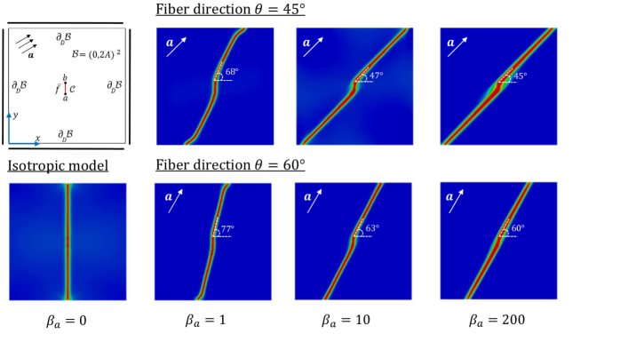
Figure 2: Influence of the different values of penalty-like parameters (here $\beta_{a}$ while $\beta_{g}=0$) in the hydraulically induced crack driven by fluid volume injection. Here, the computation domain is shown in the first plot and two different fiber direction are studied.

2.4 Numerical illustration

We now investigate the influence of the penalty-like parameters for the computed solution from (49) to the crack phase-field solution state. Here, we consider only transversely isotropic poroelastic material responses induced by the fluid volume injection. We vary the parameters for the anisotropic modeling as $\beta_{a}=1,10,200$ to represent the transverse isotropy characterized by the normal vector defined as ${\mathbf{a}}\mathrel{\mathop{\mathchar 58\relax}}=\big{(}cos(\phi),sin(\phi)\big{)}^{T}$. Also, by letting $\beta_{g}=\chi_{g}=0$ we recover the isotropic hydraulic fracture simulation. Furthermore, we fixed and set $\chi_{a}=10$, because of its negligible effect on the fracture model. Consider the boundary value problem given in Figure (2) (depicted in the first row from left). The material properties same as [65] and shown in Table LABEL:material-parameters.

To model transversely isotropic poroelastic material, structural stiffness is continuously augmented with a unidirectional fiber. We consider two cases. First, the fiber is inclined under an angle $\phi=+45^{\circ}$ while in the second one fiber is inclined under $\phi=+60^{\circ}$ with respect to the $x$-axis of a fixed Cartesian coordinate system. The two cases are shown in Figure 2 in the first row and second row, respectively.

For both cases, the first important observation is that, increasing the penalty-like parameter $\beta_{a}$ in (49) results in the fracture direction to be aligned with the highest strength direction of the poroelastic material which is ${\mathbf{a}}$. Another impacting factor that should be noted the less value for $\beta_{a}$ behave as an isotropic model (inclined vertically) that is shown in Figure (2), depicted in the second row. Note, there is very slight changes in the crack profile between $\beta_{a}=10$ and $\beta_{a}=200$.

Next, we use the anisotropic hydraulic fracture model used in Algorithm 1 and validated in this section as a departure point for the Bayesian inversion framework for the phase-field hydraulic fracture. That is described in a detail in Section 3.

3 Bayesian inversion for anisotropic phase-field hydraulic fracture

Uncertainties in the description of reservoir lithofacies, porosity, and permeability are major contributors to the uncertainties in reservoir performance forecasting. Moreover, the uncertainties in the characterization of formation properties, fracture properties, temperature effects, identification of elastic parameters, and flow mechanisms affect the productivity of wells. In this section, we introduce a computational technique based on MCMC to model the uncertainty in hydraulic fractures.

There is usually a lack of information about problem parameters and they undergo many uncertainties coming e.g. from the heterogeneity of rock formations and complicated realization of experiments for parameter identification. The Bayesian approach provides a principal framework for combining the prior knowledge with dynamic data in order to make predictions on quantities of interest. In most cases, direct measurements of the quantities is not feasible; therefore, using the forward model, an inverse approach enables us to predict these parameters with a low computational cost. As a result in addition to provide a comprehensive model that describes the fracture (crack propagation), the influential parameters are identified.

Here, we introduce a parameter estimation framework to determine different effective hydraulic fracture phase-field parameters. We consider the unknown values, i.e., elasticity modulus of the rock formation, Biot’s coefficients, fluid velocity, and the energy release rate will be components of a random vector. We first employ the statistical model

$$\mathcal{R}=\mathcal{M}(\Theta)+\epsilon.$$ (51)

• $\mathcal{R}$ is a random variable that indicates the reference value (i.e., reference observation or measured data).

• $\mathcal{M}$ points out a PDE-based model (here the hydraulic phase-field model i.e., (50)). The variable $\Theta$ is a random field and denotes the realizations of random variables (here the unknown material parameters, denoting $\Theta\in\{\lambda,\mu,B,M,\eta_{F},G_{c},\beta_{a},\beta_{g}\}$, see Subsection 3.2 for the physical interpretation). In total, $\mathcal{M}(\Theta)$ relates to the solution of the model according to a given set of parameters. Here, we focus on the scalar-valued maximum pressure, that is

  $$\mathcal{P}\mathrel{\mathop{\mathchar 58\relax}}=\max_{\mathcal{B}}\{p\},$$ (52)

  at a fixed fluid injection time. This value indicates an observation with respect to a given set of parameters ($\theta\in\Theta$). In other words, by solving the system of equations (50) (using $\theta$), the function $\mathcal{M}$ transfers the material unknowns to an observation (here $\mathcal{P}$) which shows the fracture behavior. We should note that the function $\mathcal{M}\mathrel{\mathop{\mathchar 58\relax}}\mathbb{R}^{n_{r}}\mathrel{\mathop{\mathchar 58\relax}}\rightarrow\mathbb{R}^{n_{m}}$, where $n_{r}$ is the dimension of the unknown parameters and $n_{m}$ is the dimension of the reference observation (here $\mathcal{P}$).

• $\epsilon$ is the estimation error and arises from uncertainties in experimental situations and denotes a sample of $\mathcal{N}(0,\sigma^{2}I_{n_{r}})$, where $\mathcal{N}$ is the normal distribution and $\sigma^{2}$ denotes a fidelity parameter.

Several Markov chain Monte Carlo techniques, e.g., Metropolis-Hastings (MH) [66] or more effective methods such as the delayed-rejection adaptive-Metropolis method are employed to determine the posterior density of the parameters.

Generally, for a sample $\theta$ of the random field $\Theta$ indicating a realization of the parameters (given in Subsection 3.2) related to a sample $r$ of the observations $\mathcal{R}$, the posterior density is expressed as

$$\pi(\theta|r)=\frac{\pi(r|\theta)\pi_{0}(\theta)}{\pi(r)}=\frac{\pi(r|\theta)\pi_{0}(\theta)}{\displaystyle\int_{\mathbb{R}^{n_{r}}}\pi(r|\theta)\pi_{0}(\theta)\,d\theta},$$ (53)

where $\pi_{0}(\theta)$ denotes the prior distribution (prior information) and $\mathbb{R}^{n_{r}}$ indicates the parameters space (a normalization parameter) and its estimation is not computationally easy. Hence, we estimate the posterior density neglecting the normalization constant leads to

$$\pi(\theta|\,r)\propto\pi(r|\,\theta)\pi_{0}(\theta).$$

To estimate the posterior density in the above relation which is the probability density of a set of unknown parameters, the likelihood function $(\pi(r|\theta))$ should be formulated. The likelihood function reads

$$\pi(r|\theta)\mathrel{\mathop{\mathchar 58\relax}}=\frac{1}{(2\pi\sigma^{2})^{\bar{n}/2}}\exp\left(-\zeta(\theta)/2\sigma\right),\qquad\text{with}\qquad\zeta(\theta)=\sum_{i=1}^{n}(r_{i}-\mathcal{M}(\theta))^{2},$$ (54)

where $n$ is the number of time-steps. Here, for a given realization $\theta$ (a set of parameters), higher $\zeta(\theta)$ (more difference between the model solution and the observation) gives rise to a lower likelihood estimation (lower probability). On the other hand, a negligible difference leads to maximum likelihood estimation and a probability close to 1. We choose also the reference observation by a fine mesh to perform the test problems. We observe the dependence of maximum pressure ($\mathcal{P}$) to different effective parameters (listed in Subsection 3.2). Obviously, the observation can be modified (more precise) by using a measured value.

In MH algorithms, during every sampling, a new candidate $\theta^{*}$ based on the proposal density (e.g., uniform or Gaussian) $\phi$ is proposed, and its acceptance rate (denoted by $\lambda_{1}$) concerning the previous candidate (here $\theta^{k-1}$) is computed. The ratio is given as follows:

$$\lambda_{1}(\theta^{*}|\,\theta^{k-1})\mathrel{\mathop{\mathchar 58\relax}}=\min\left(1,\cfrac{\pi(\theta^{*}|\,r)~{}\phi(\theta^{k-1}|~{}\theta^{*})}{\pi(\theta^{k-1}|\,r)~{}\phi(\theta^{*}|\,\theta^{k-1}))}\right).$$ (55)

A high acceptance ratio means the proposed proposal gets simulation results closer to the (reference) observation; therefore, it will be accepted; otherwise, the algorithm rejects the candidate (if the ratio is low).

3.1 The DRAM algorithm for hydraulic fracture

$\bullet$ Produce an initial $\theta^{0}\sim\pi(\theta^{0}|\,r)$ value ($k=0$)   
for $k=1,\ldots,N$

$\bullet$ set FLAG=true     $\bullet$ set $n=0$

1. Propose a new proposal $\theta^{*}=\theta^{k-1}+\mathcal{D}_{k}\mathcal{Z}_{k}$.

while FLAG  do

I. Solve the system of equations (i.e., $\mathcal{E}_{{\Bgothic U}}({\Bgothic U},\delta{\Bgothic U})=0$, see (50)) using Algorithm 1
             and obtain $(\bm{u},p,d)$ according to the realization $\theta^{*}\in\{\mu,K,M,B,G_{c},\eta_{F},\beta_{a},\beta_{g}\}$.

II. Estimate the maximum of the pressure in the geometry $\mathcal{P}=\text{max}(p)$

III. if $d$ reaches the boundary

IV. else if $t_{n}>T$ then     $\bullet$ set FLAG=false

V.  else   $\bullet$  set $n+1\rightarrow n$   $\bullet$  set $t_{n}=n\Delta t$

2. Calculate the acceptance/rejection probability

$$\lambda_{1}(\theta^{*}|\,\theta^{k-1})=\min\left(1,\cfrac{\pi(\theta^{*}|\,r)~{}\phi(\theta^{k-1}|~{}\theta^{*})}{\pi(\theta^{k-1}|\,r)~{}\phi(\theta^{*}|\,\theta^{k-1}))}\right)$$

.

3. if  $\mathcal{RV}<\lambda_{1}~{}$ then accept the proposal $\theta^{*}$ and put $\theta^{k}=\theta^{*}$ else

I. Calculate the alternative proposal  $\theta^{**}=\theta^{k-1}+\sigma^{2}\mathcal{D}_{k}\mathcal{Z}_{k}$ .

II.  $\bullet$ set FLAG=true     $\bullet$ set $n=0$

$\bullet$ obtain new $\mathcal{P}$ (see the while/do loop) according to the realization $\theta^{**}$

III. Calculate the acceptance/rejection probability of the delayed rejected candidate

$$\qquad\qquad\lambda_{2}(\theta^{**}|\,\theta^{k-1},\theta^{*})=\min\left(1,\cfrac{\pi(\theta^{**}|\,r)~{}\phi(\theta^{*}|~{}\theta^{**})\left(1-\lambda_{1}(\theta^{*}|\theta^{**})\right)}{\pi(\theta^{k-1}|\,r)~{}\phi(\theta^{*}|~{}\theta^{k-1})\left(1-\lambda_{1}(\theta^{*}|\theta^{k-1})\right)}\right)$$

.

IV. if  $\mathcal{RV}<\lambda_{2}$  then  accept the proposal $\theta^{**}$ and put $\theta^{k}=\theta^{**}$

V.   else   $\bullet$ reject the proposal $\theta^{**}$ and put $\theta^{k}=\theta^{k-1}$    

4. Update the covariance matrix as $\mathcal{V}_{k}=\text{Cov}(\theta^{0},\theta^{1},\ldots\theta^{k})$.

5. Update $\mathcal{D}_{k}$

end

Algorithm 2 The DRAM algorithm for anisotropic hydraulic phase-field fracture.

The Metropolis-Hastings technique is a robust and efficient MCMC technique to estimate the posterior density. Its efficiency verified by the authors in [50] to identify mechanical coefficients (mechanical parameters and the critical energy rate). Despite its efficiency, during the iterations, the covariance function of the proposal should be tuned manually, and the method has a high autocorrelation. To overcome these drawbacks, during each sampling, the covariance based on the existing samples (adaptive Metropolis) is updated; therefore, the posterior density is not sensitive to the proposal density. We can modify the technique additionally by using a delayed rejection. To this end, a replacement of the rejected proposal is obtained (i.e., $\theta^{**}$); then, the new acceptance/rejection probability (denoted by $\lambda_{2}$) is computed, that is

$$\qquad\qquad\lambda_{2}(\theta^{**}|\,\theta^{k-1},\theta^{*})=\min\left(1,\cfrac{\pi(\theta^{**}|\,r)~{}\phi(\theta^{*}|~{}\theta^{**})\left(1-\lambda_{1}(\theta^{*}|\theta^{**})\right)}{\pi(\theta^{k-1}|\,r)~{}\phi(\theta^{*}|~{}\theta^{k-1})\left(1-\lambda_{1}(\theta^{*}|\theta^{k-1})\right)}\right).$$ (56)

In other words, a second-stage move will be used to increase the acceptance chance of the rejected proposal. The algorithm is useful, specifically when the samples have a high-dimensional conditional density [67].

The DRAM algorithm for parameter estimation in hydraulic fracture is summarized in Algorithm 2. Here, $\mathcal{Z}_{k}\sim\text{Uniform}~{}(0,I_{n_{r}})$ where $I_{n_{r}}$ denotes the $n_{r}$-dimensional identity matrix, $\mathcal{D}_{k}$ indicates the Cholesky decomposition of $\mathcal{V}_{k}$ (the covariance of the realizations), and $\mathcal{RV}\sim\text{Uniform}~{}(0,1)$. To enhance the acceptance rate, we update the covariance function of the proposal density. In order to provide a narrower proposal density, we use $\sigma<1$. The covariance function can be estimated by

$$\text{Cov}(\theta^{0},\theta^{1},\ldots,\theta^{k})=\frac{1}{k}\left(\sum_{i=0}^{k}\theta^{i}\left(\theta^{i}\right)^{T}-(k+1)~{}\hat{\theta}^{k}\left(\hat{\theta}^{k}\right)^{T}\right),$$ (57)

where $\hat{\theta}^{k}=\frac{1}{k+1}\displaystyle\sum_{i=0}^{k}\theta^{i}$.

3.2 Physical interpretation of the parameters

Here we review the list of important parameters (with their used unit) in hydraulic fracture and explain that are they correlated or not.

• Elasticity modulus [GPa]. Generally, the mechanical material parameters denote the shear modulus $\mu$ and Lamé’s first parameter $\lambda$. The bound $\lambda>-\frac{2\mu}{3}$ may relate it to the shear modulus. Poisson’s ratio $\nu$ also satisfies the condition $-1<\nu<\frac{1}{2}$. Hence, these two parameters are not well-suited for the estimation due to their bounds and dependency. Instead, the effective bulk modulus, $K=\lambda+\frac{2\mu}{3}$ in addition to the shear modulus are chosen as the elasticity parameters. Therefore, the only necessary constraint is the positivity of the parameters. Since the mechanical parameters are correlated a joint probability density will be estimated.

  Higher shear modulus (due to higher Young’s modulus) increases the reservoir hardness; therefore, the fracture initiates faster and the propagation rate is more for the cases with higher Young’s modulus. The bulk modulus is the measure of the decrease in volume with an increase in pressure.

• Biot’s coefficient $B$ described by Biot [68] and represents the change of the bulk volume because of a pore pressure change while the stress is constant (the contribution of the pore pressure to the stress). The fracture length reduces with a raise in the Biot’s number. The effect of the pore pressure on the fracture propagation can be more pronounced for higher Biot’s coefficient [69].

• Biot’s modulus $M$ [GPa] considers the combined fluid/solid compressibility. The inverse of $M$ denotes the rate of the volume of fluid released from a non-deforming frame to the pore pressure drop, therefore determines a storage coefficient [70].

• Dynamic fluid viscosity $\eta_{F}$ [kg/(m.s)] is the resistance to movement of one layer of a fluid over another. By raising dynamic viscosity, the breakdown pressure rises noticeably however the fracture initiation pressure rises only slightly.

• Griffith’s critical energy release rate $G_{c}$ [GPa] indicates a property of the materials that the fracture is propagating in or into. In other words, it is represented as the decline in total potential energy per increase in fracture surface area.

Due to the nature of subsurface systems, it is hard and time-consuming to provide the measurements for the inverse problem. Considering the limited resources, it is useful to choose the reference value, via a simulation-based technique. To that end, the quantity of interest in our simulation is the maximum fluid pressure versus the fluid injection time. Findings [22, 71, 21] showed that maximum pressure increases within the fractured area before the onset of the crack propagation, which yields into a drop of the fluid pressure, that is well-know observation in the fracking process [22].

The typical random distribution of the unknown parameters is log-normal. Hence, in the Bayesian inverse framework, it is usual to work with their logarithms (i.e., natural logarithm) instead of the original variables and to choose Gaussian distribution as the prior distribution. With that, we can remove the positivity constraint as well.

4 Numerical experiments

In this section, to use the developed numerical procedure for modeling hydraulic fractures in isotropic and anisotropic solids, we employ four specific numerical examples. The used material parameters are given in Table LABEL:material-parameters (according to [30, 65]). To obtain the solution of the coupled system of equations bilinear quadrilateral $Q1$ finite elements are used, and the consistent linearization, including finite element discretization, is further explained in detail in Appendix A.

Table 1: Material parameters employed in the numerical experiments according to [30, 65].

No.	parameter	name	value	unit
1.	$\mu$	shear modulus	$6.65$	$\mathrm{GPa}$
2.	$K$	bulk modulus	$11$	$\mathrm{GPa}$
3.	$M$	Biot’s modulus	$12.5$	$\mathrm{GPa}$
4.	$B$	Biot’s coefficient	$0.79$	–
5.	$K_{D}$	Intrinsic permeability	$2\times 10^{-14}$	$\mathrm{m^{2}}$
6.	$\zeta$	Permeability transition exponent	$50$	–
7.	$\eta_{F}$	Dynamic fluid viscosity	$0.001$	$\mathrm{kg/(m.s)}$
8.	$G_{c}$	Griffith’s energy release rate	$0.00265$	$\mathrm{GPa}$
9.	$\eta$	Crack viscosity	$10^{-14}$	$\mathrm{N/m^{2}s}$
10.	$\kappa$	Stabilization parameter	$10^{-8}$	–

Here, we introduce four different numerical experiments. Then, we employ the DRAM technique to identify the influential parameters. The first two examples cover only isotropic materials, where in the next two problems we consider transversely isotropic and orthotropy anisotropic fractures. In the DRAM algorithm, we employ the fidelity parameter $\sigma=10^{-3}$ and we replicate the Bayesian algorithm for $N=10\,000$ number of samples. In all examples, $h=1/200$ is used for the simulations and $h=1/215$ is employed to obtain the reference observation (using the given values in Table LABEL:material-parameters). A length scale of $l=2h$ in addition to a negligible $\kappa$ (here is $10^{-8}$) is used as well. Regarding the stabilization parameter, we refer the reader to [50] for a discussion. Finally, for all examples, the prior distribution of all desired parameters are listed in Table LABEL:prior.

Table 2: The prior distribution of the model parameters for different test problems.

parameter	prior distribution	true value	test problems
$B$	$\mathcal{N}(0.8,0.1)$	0.79	all
$\eta_{F}$	$\mathcal{N}(0.001,0.0001)$	0.001	all
$G_{c}$	$\mathcal{N}(0.0027,0.0003)$	$0.00265$	all
$\mu$	$\mathcal{N}(6.5,0.5)$	$6.65$	all
$K$	$\mathcal{N}(11,1)$	11	all
$M$	$\mathcal{N}(12,1)$	$12$	all
$\beta_{a}$	$\mathcal{N}(50,60)$	55	Example 3
$\beta_{a}$ or$~{}\beta_{g}$	$\mathcal{U}(0,2)$	0.5	Example 4, Case b
$\beta_{a}$ or$~{}\beta_{g}$	$\mathcal{U}(0,20)$	10	Example 4, Case b
$\beta_{a}$ or$~{}\beta_{g}$	$\mathcal{U}(0,20)$	10	Example 4, Case d
$\beta_{a}$ or$~{}\beta_{g}$	$\mathcal{U}(150,250)$	200	Example 4, Case d

4.1 Hydraulically induced crack driven by fluid volume injection

In the following numerical example, a BVP is applied to the square plate shown in Figure 3(a). We set $A=40~{}m$ hence $\mathcal{B}=(0,80)^{2}~{}m^{2}$ that includes a predefined single notch $\mathcal{C}_{1}$ of length $8~{}m$ in the body center with $a=(36,40)\;m$ and $b=(44,40)\;m$, as depicted in Figure 3(a). A constant fluid flow of $\bar{f}=0.003\;m^{2}/s$ is injected in $\mathcal{C}_{1}$. At the boundary $\partial_{D}\mathcal{B}$, all displacements are fixed in both directions and the fluid pressure is set to zero. Fluid injection $\bar{f}$ continues until failure for $T=60$ second with time step $\Delta t=0.1$ second during the simulation. In the next two examples, we deal with isotropic hydraulic fracture and hence we fixed and set $\beta_{a}=\chi_{a}=\beta_{g}=\chi_{g}=0$ to recover isotropic formulation.

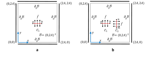
Figure 3: Geometry and boundary conditions (a) Example 1. Hydraulically induced crack driven by fluid volume injection, and (b) Example 2. Joining of two cracks driven by fluid volume injection.

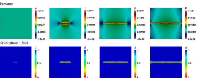
Figure 4: Example 1. Reference results of the hydraulically induced crack driven by fluid volume injection. Evolution of the fluid pressure $p$ (first row) and crack phase-field $d$ (second row) for different deformation stages up to the final failure at $t=0.1,\,6.5,\,30,\,49.5$ seconds.

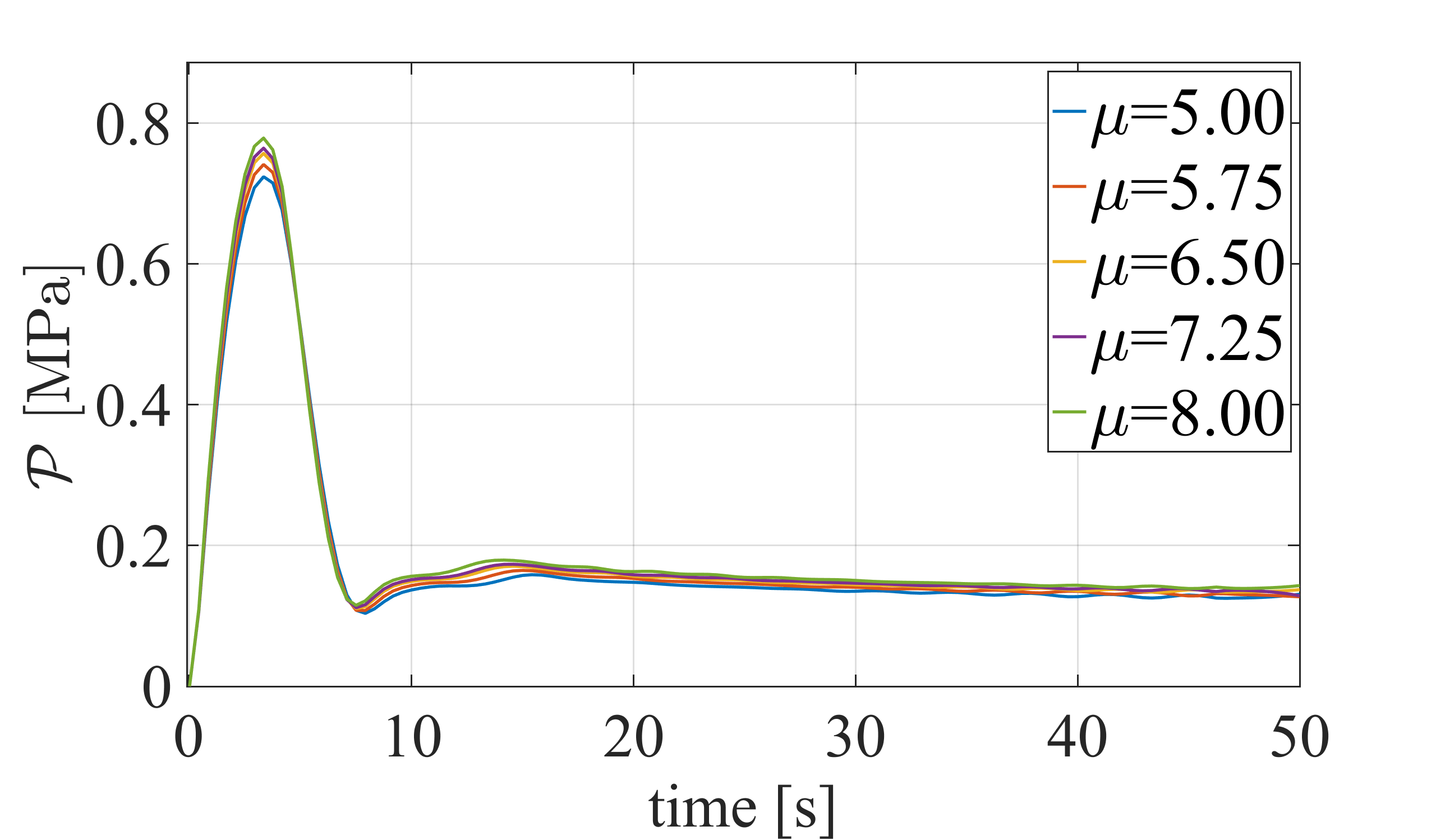
(a)

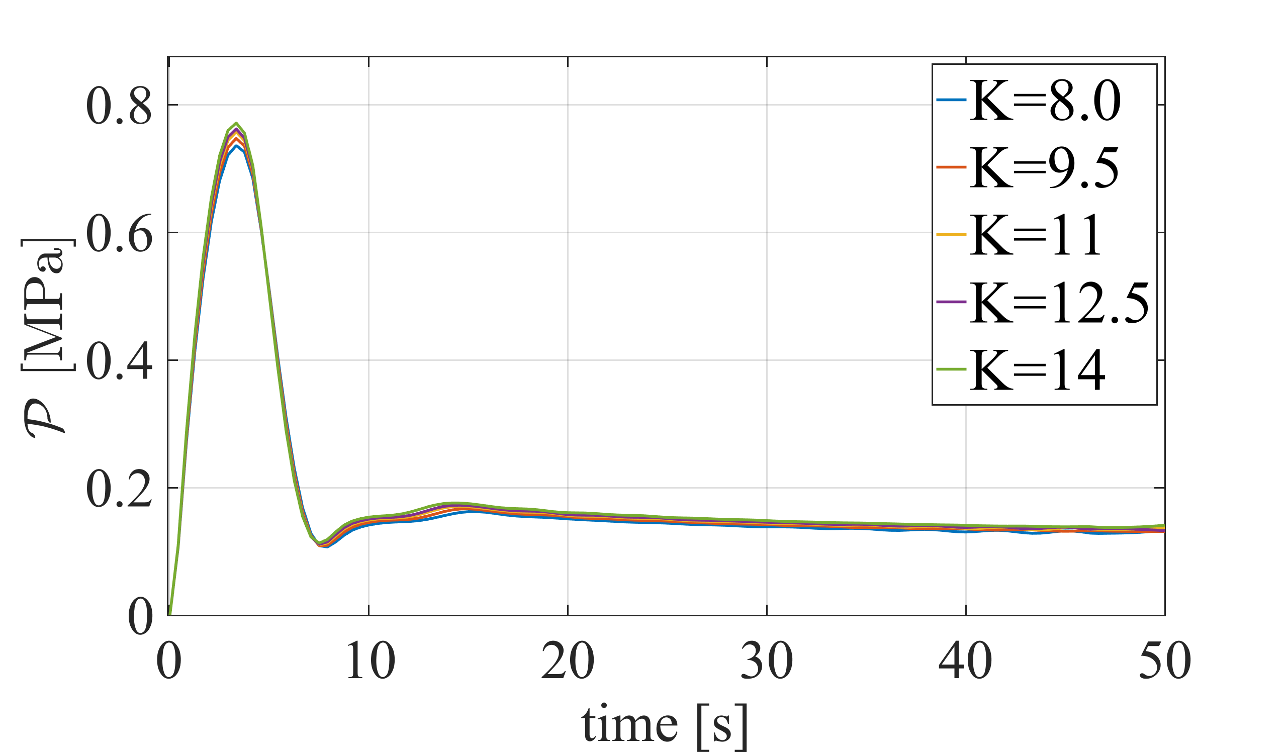
(b)

(c)

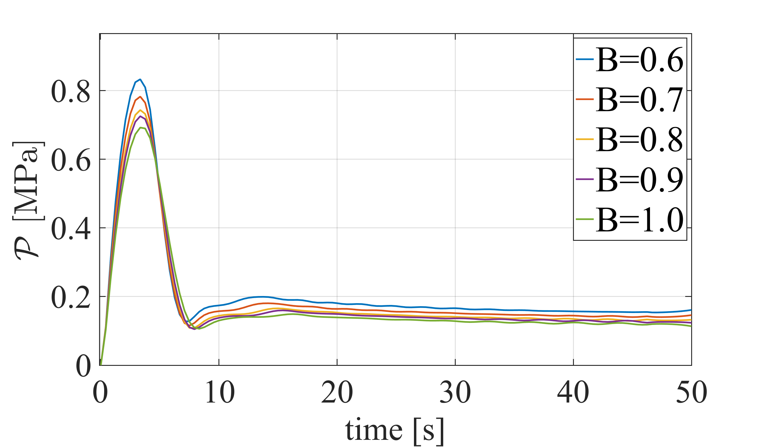
(d)

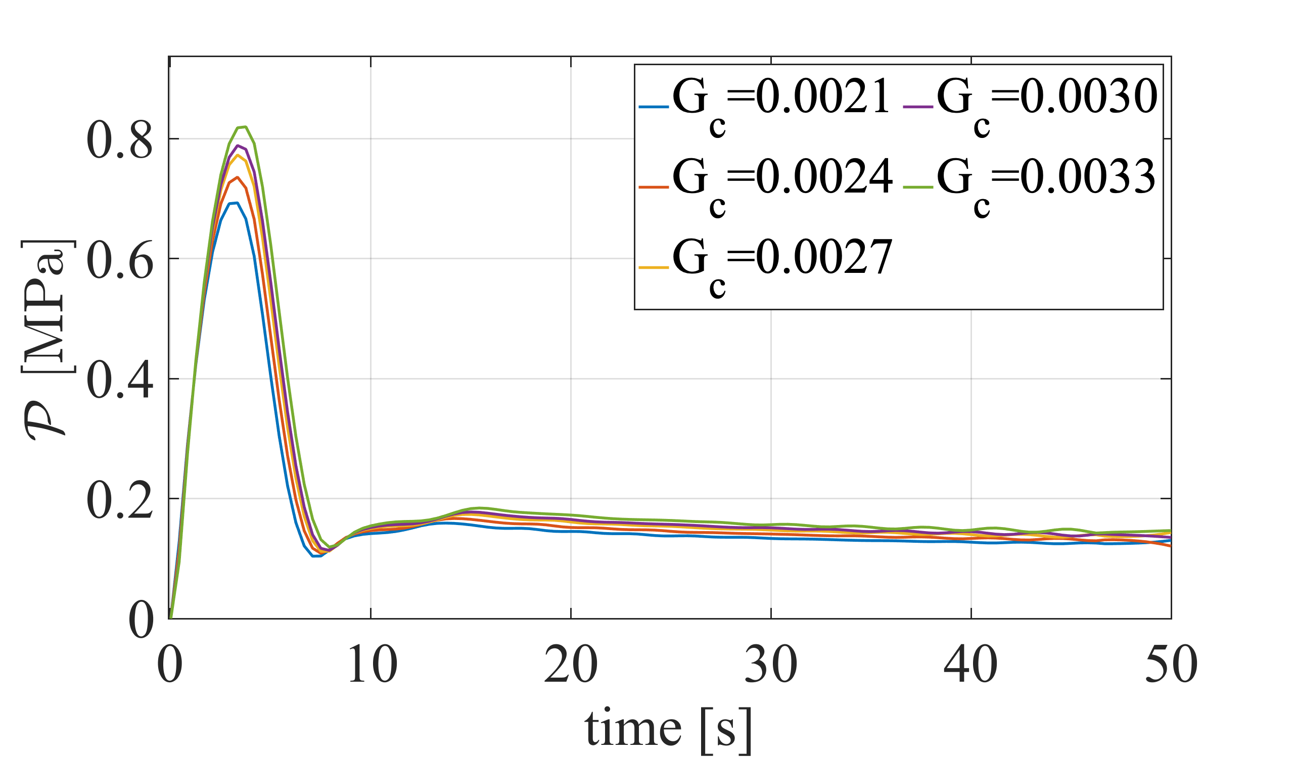
(e)

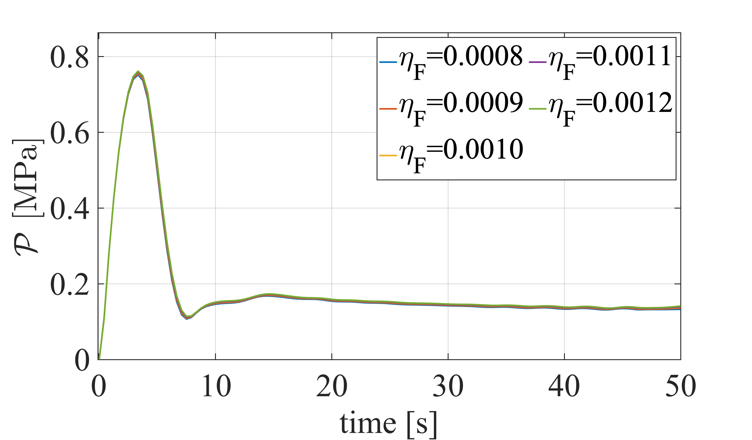
(f)

Figure 5: Example 1. The maximum pressure value $\mathcal{P}$ for different values of $\mu$, $K$, $M$, $B$, $G_{c}$, and $\eta_{F}$.

We start our analysis by illustrating the reference results for different fluid injection time up to final failure related to Figure 3a. The fluid pressure $p$ (first row) and crack phase-field $d$ (second row) evolutions are demonstrated in Figure 4 for four-time steps, i.e., $t=0.1,\,6.5,\,20,\,34.5$ seconds. The crack initiates at the notch-tips due to fluid pressure increase. Thereafter, the crack propagates horizontally in two directions towards the boundaries. In the fractured zone, $p$ is almost constant due to the increased permeability inside the crack. Whereas, low fluid pressure in the surrounding is observed due to the chosen small time-step in comparison with the permeability of the porous medium, as outlined in [30]. The fluid pressure drops down while the crack propagates further as shown in Figure 4(b) (second row, middle states). Then, $p$ increases again due to the prescribed fixed boundary conditions $\partial_{D}\mathcal{B}$, see Figure 4 (first row, last state).

Figure 5 shows the pressure curve during the injection time for different values for six influential parameters. As the figure shows, an increase in the Biot’s coefficient raises the pressure peak point; however, for the rest of the parameters, it gives rise to a decline. We continued the pressure estimation until the crack reached the boundary (here $T=60$ seconds is used).

Now the Bayesian inversion (the DRAM technique) is employed to identify the parameters. Figure 6 depicts the histogram of posterior density of the values. Due to the correlation of the parameters, the joint probability of the elastic modulus and Biot’s coefficient/modulus are estimated. As shown, a wide probability density for $\eta_{F}$ indicates its low impact on the pressure; however, the narrow curve for $G_{c}$ points out its high effect on the pressure during the injection time. The results are compatible with the obtained curves in Figure 5.

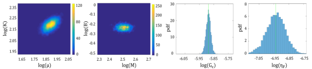
Figure 6: Example 1. From left to right: the posterior density of the mechanical parameters, Biot’s coefficients/modulus, $G_{c}$, and $\eta_{F}$. The green lines are the mean values.

The main advantage of the DRAM algorithm compared to the Metropolis-Hastings algorithm in phase-field fracture [50] is a significantly higher acceptance rate. As we already mentioned, the proposal adaptation and the new adjusted candidate improves the reliability/efficiency of the parameter identification. In order to verify the obtained values, we solved the system with the posterior knowledge and estimated $\mathcal{P}$. Figure 7 illustrates the pressure diagram obtained by the prior and posterior values and the chosen reference observation. The technique efficiency in the precise estimation of the peak point and curve behavior can be observed here.

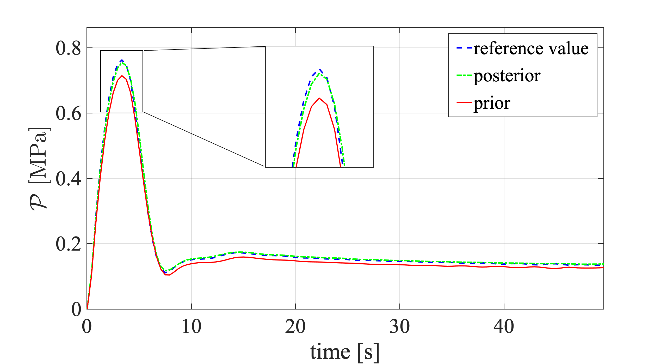
Figure 7: Example 1. A comparison between the maximum pressure (during the injection time) with prior values (red line) and the posterior values (green line). The reference diagram is depicted with a blue line.

4.2 Joining of two cracks driven by fluid volume injection

The second example is given for handling coalescence and merging of crack paths for the hydraulic fracturing material. Crack-initiation and curved-crack-propagation, representing a mixed-mode fracture, are predicted with a phase-field formulation.

The boundary value problem is similar to the benchmark problem of [18] and depicted in Figure 3(b). We keep all parameters and loading as in the previous example. The first crack $\mathcal{C}_{1}$ is located near the middle of the domain with coordinates $a=(28,40)$ and $b=(36,40)$. The second crack $\mathcal{C}_{2}$ is vertically-oriented at $n=(50,44)$ and $m=(50,36)$ with a distance of $14\;m$ from $\mathcal{C}_{1}$. A constant fluid flow of $\bar{f}=0.003\;m^{2}/s$ is injected in $\mathcal{C}_{1}$ and $\mathcal{C}_{2}$ as sketched in Figure 3(b). At the boundary $\partial_{D}\mathcal{B}$, all the displacements are fixed in both directions and the fluid pressure is set to zero. Fluid injection $\bar{f}$ continues until failure for $T=28$ second with time step $\Delta t=0.1$ second during the simulation.

Figure 8 shows the evolutions of the fluid pressure $p$ (first row) and the crack phase-field $d$ (second row) for the reference problem at different times $t=1.8,\,6.5,\,13.5,\,27.7$ seconds. Here the crack propagates from the notches. We again observe nearly constant fluid pressure in the fractured area ($d=0$), whereas outside the crack zone $p$ is much lower, see Figure 8 (first row).

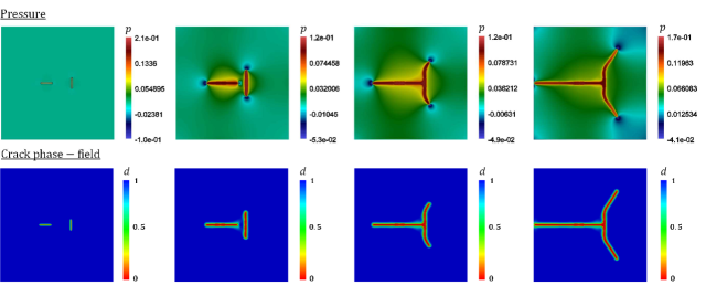
Figure 8: Example 2. Reference results of the joining cracks driven by fluid volume injection. Evolution of the vertical displacement $u_{y}$ (first row), fluid pressure $p$ (second row) and crack phase-field $d$ (third row) for different deformation stages up to final failure at $t=1.8,\,6.5,\,13.5,\,27$ seconds.

In order to study the parameter effect, we observe the pressure curve with different values of the effective parameters. Figure 9 show the influence of on $\mathcal{P}$ diagram during different injection time. The obtained information from the DRAM algorithm (the posterior distribution) is shown in Figure 11. As depicted, $G_{c}$ shows a Gaussian distribution and $\eta_{F}$ has a skewed distribution. Finally, the pressure diagram for prior/posterior and the used reference observation (with finite element mesh size ${h=0.24}$) is shown in Figure 11. Similar to Example 1, employing Bayesian inference enables us to have a more exact model, i.e., the peak point and pressure behavior are predicted more precisely.

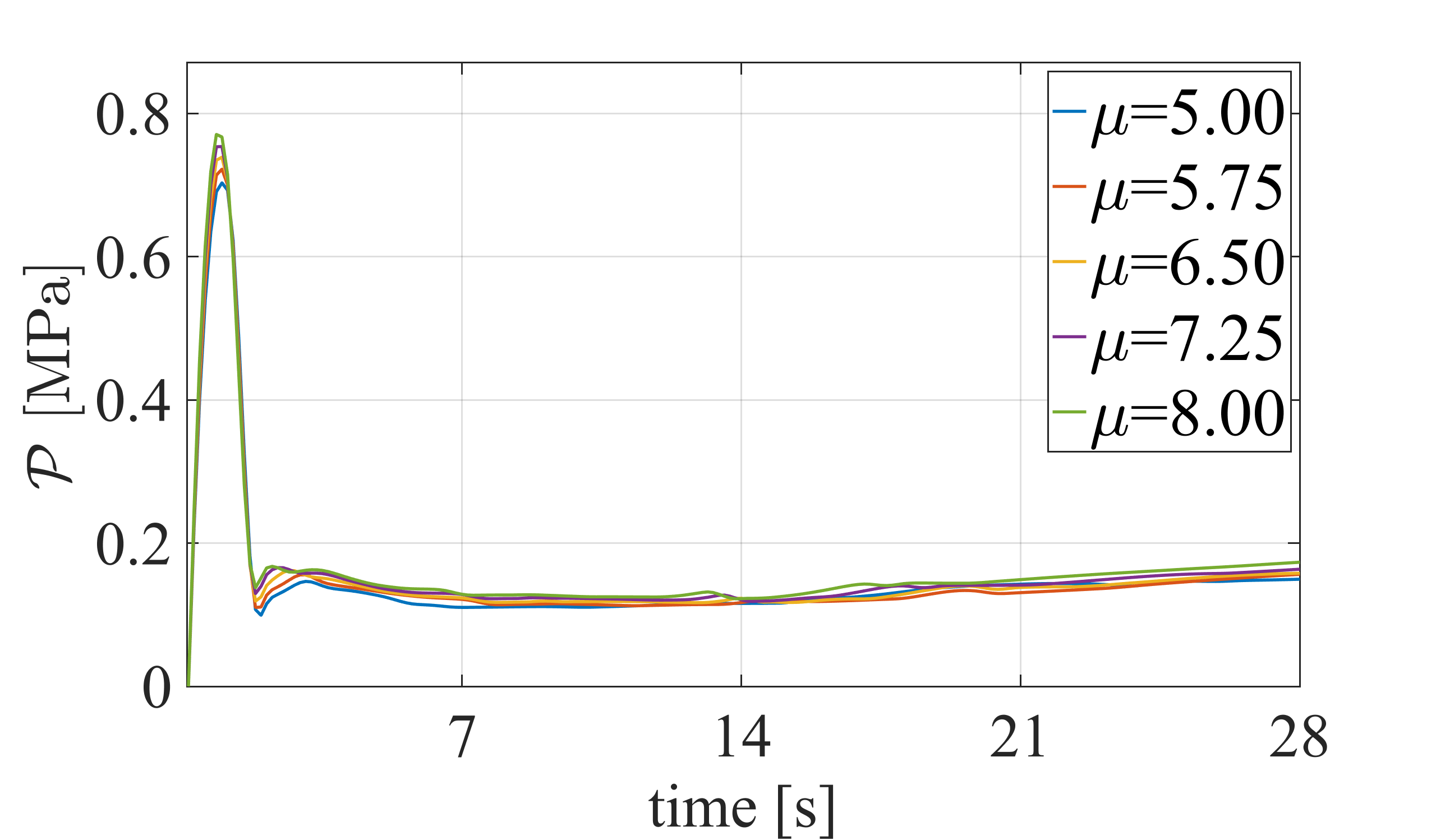
(a)

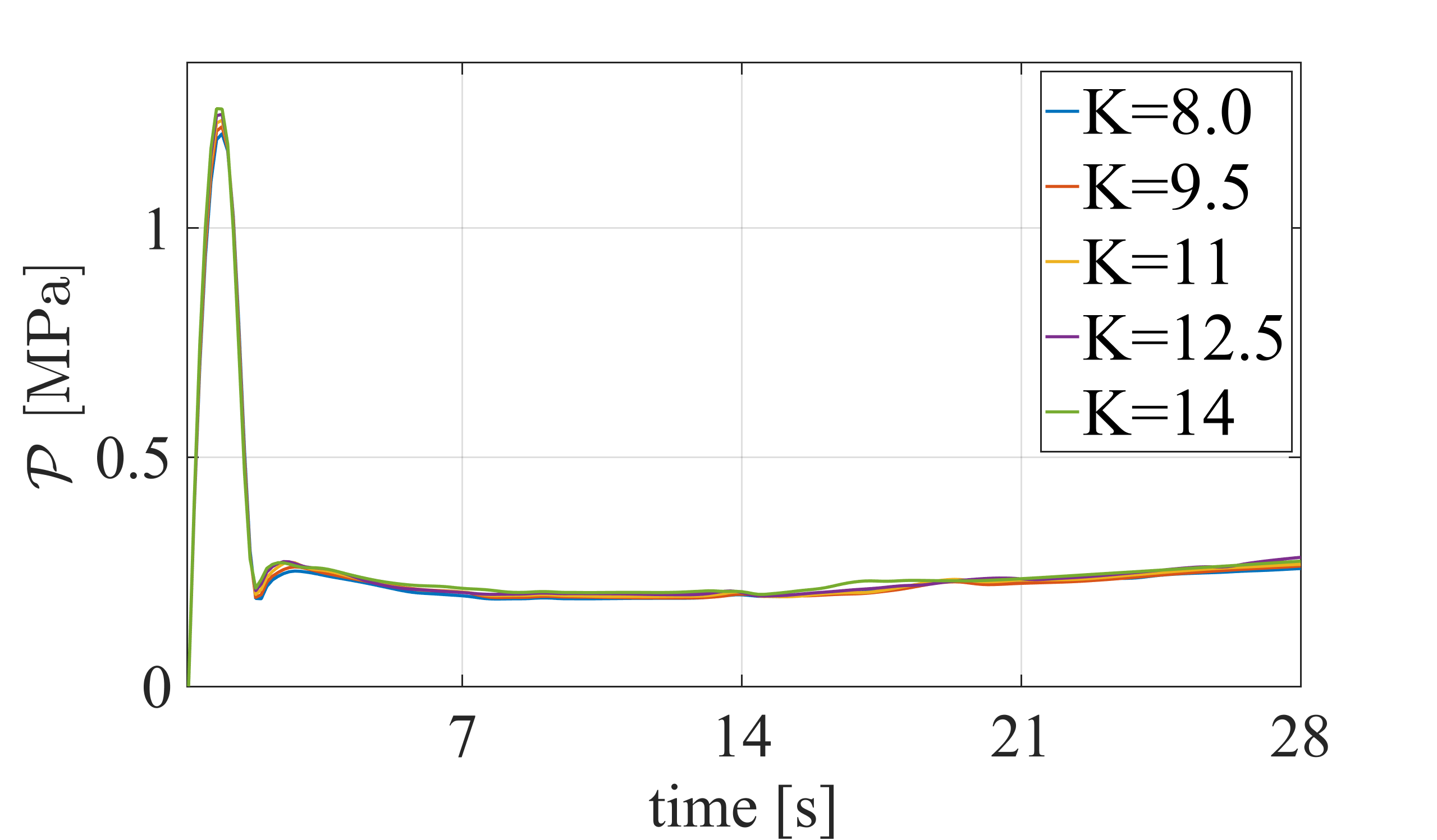
(b)

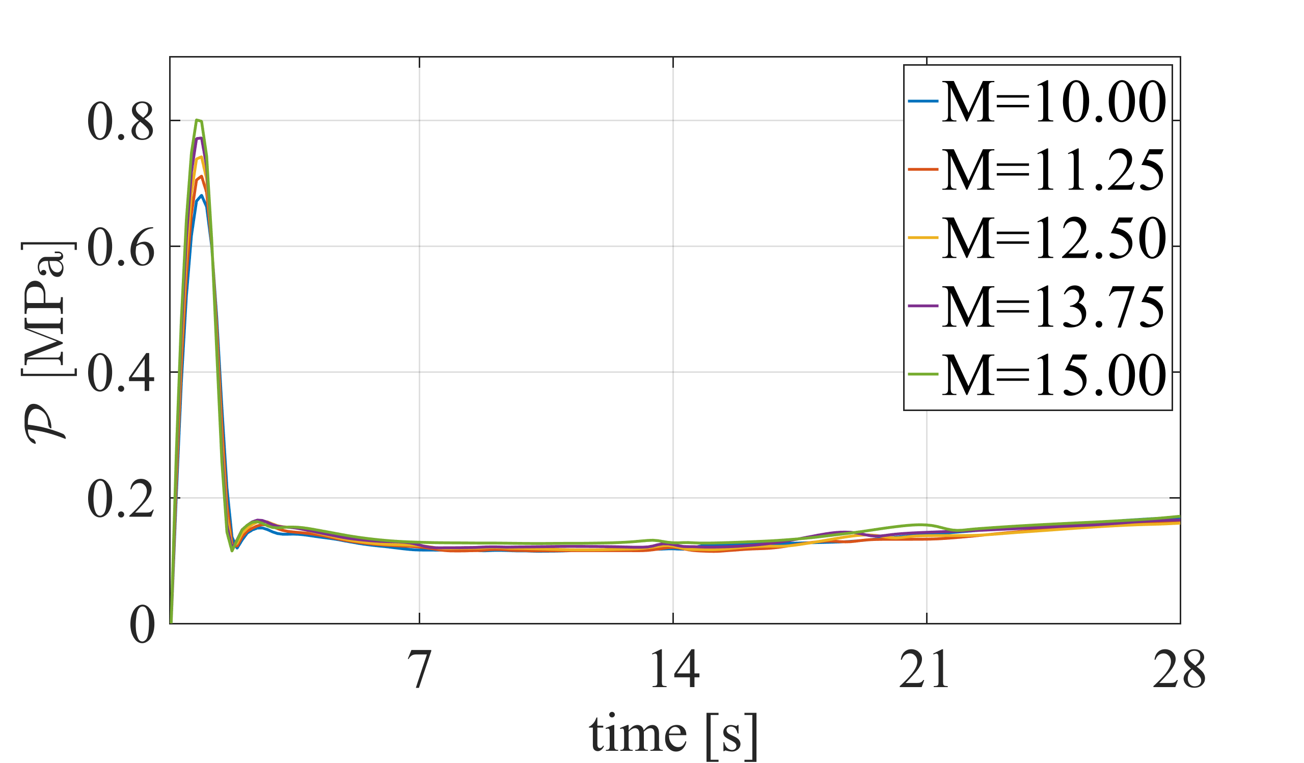
(c)

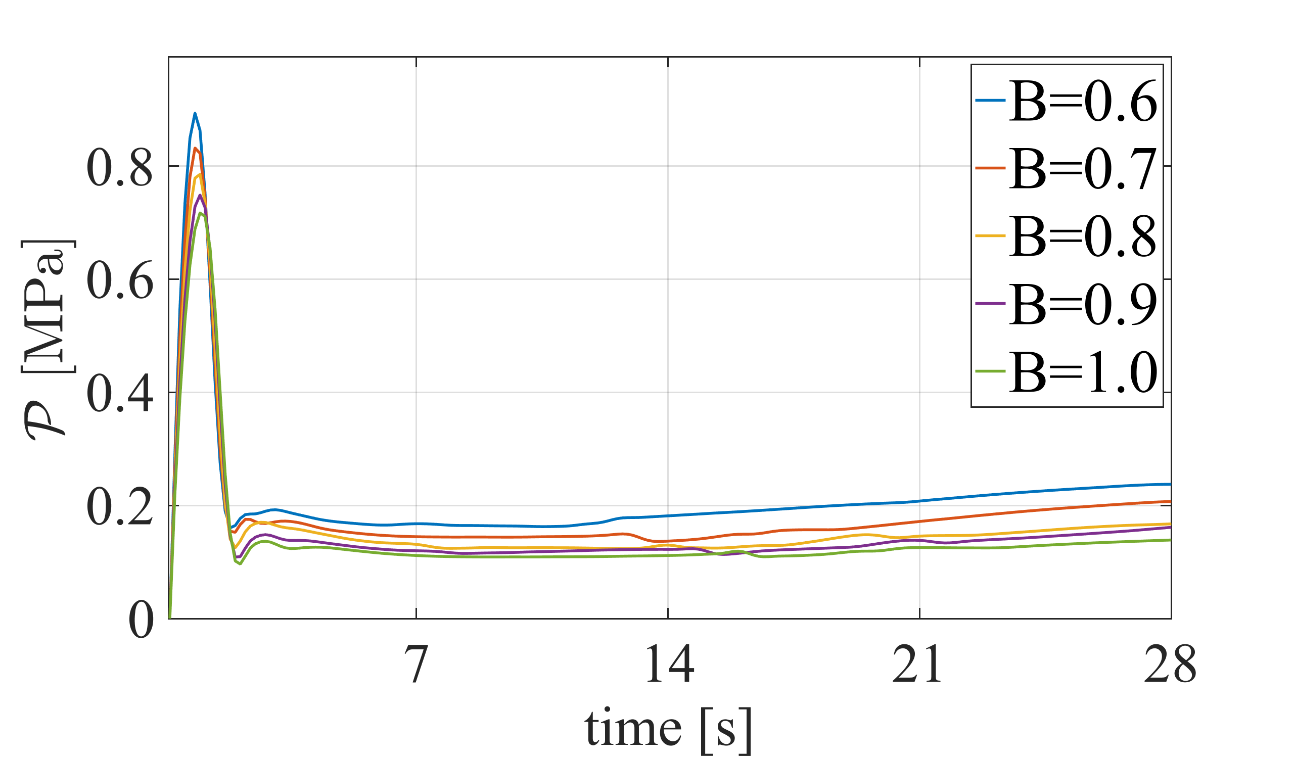
(d)

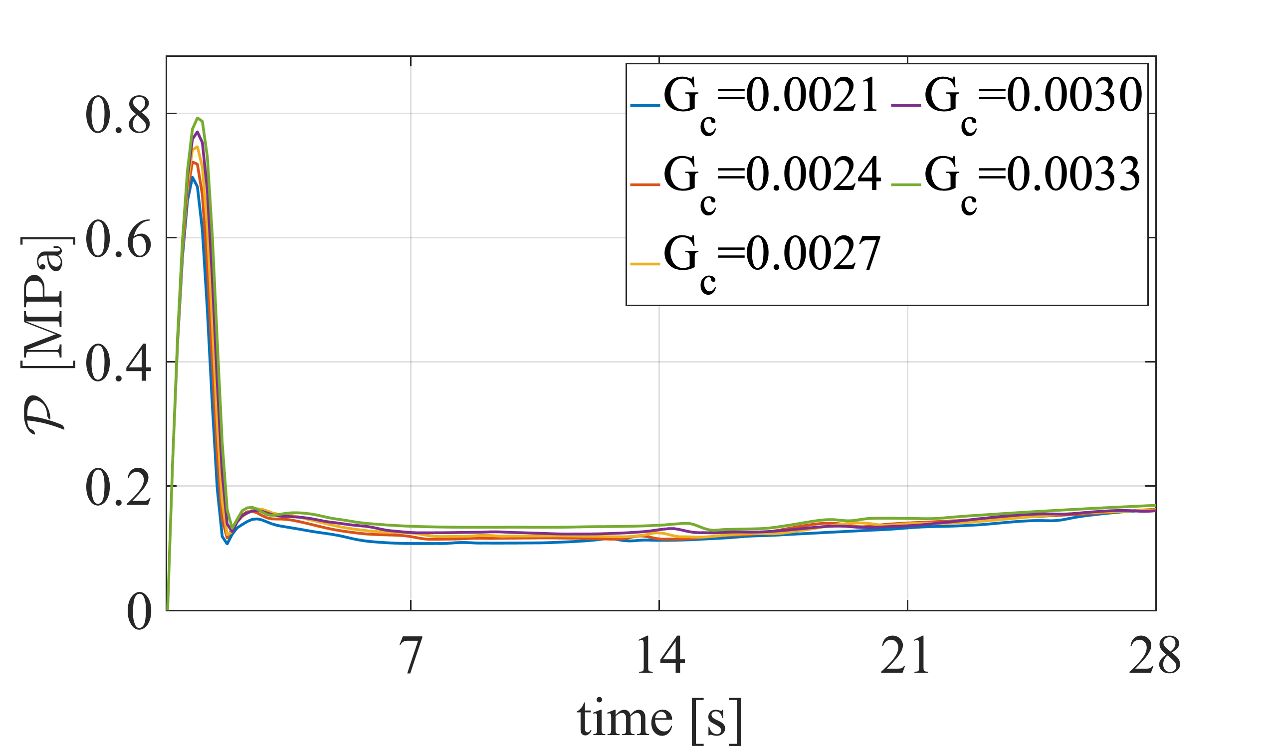
(e)

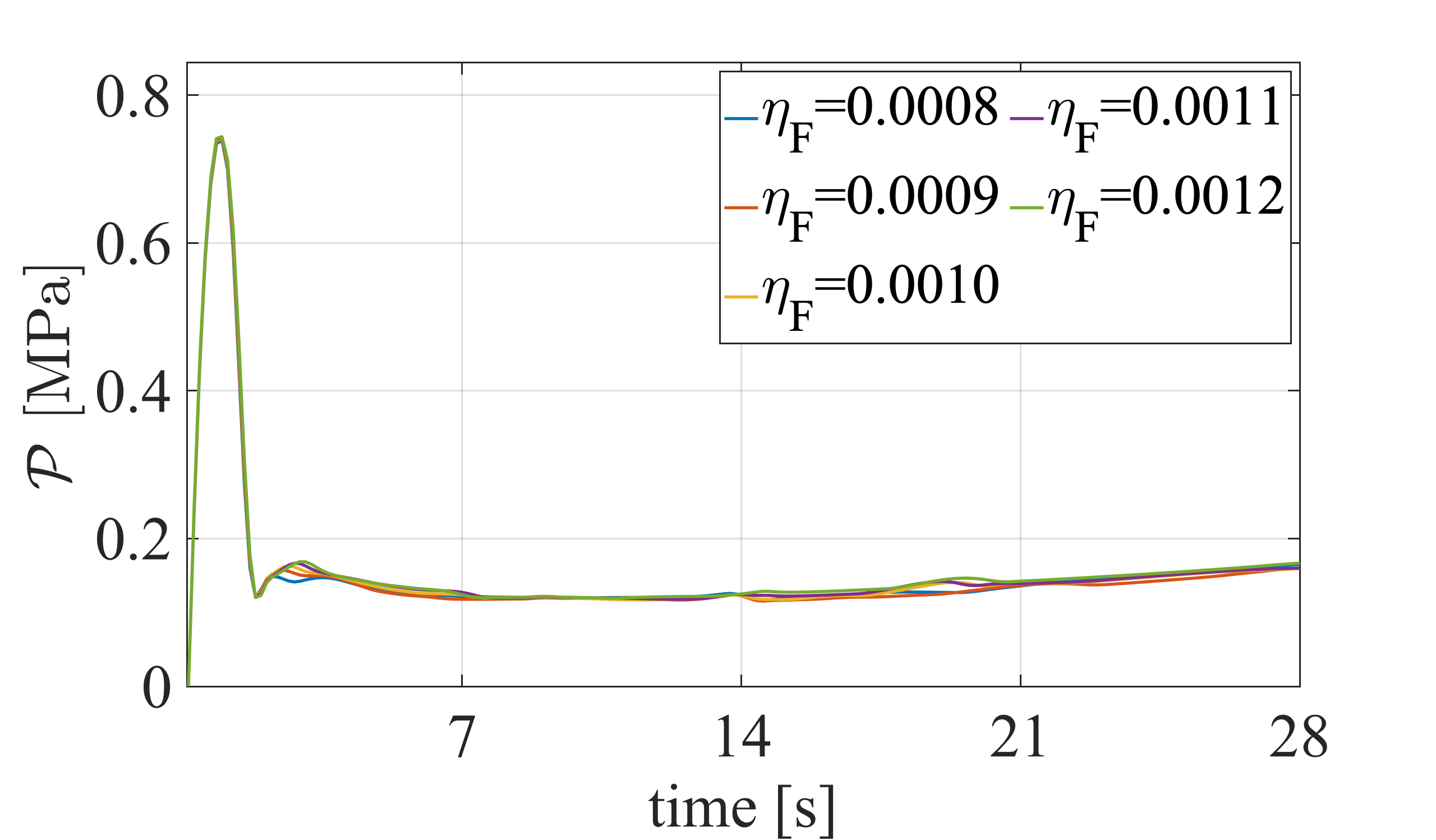
(f)

Figure 9: Example 2. The maximum pressure value $\mathcal{P}$ for different values of $\mu$, $K$, $M$, $B$, $G_{c}$, and $\eta_{F}$.

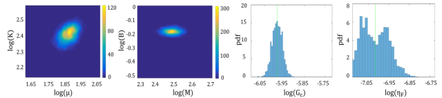
Figure 10: Example 2. From left to right: the posterior density of the mechanical parameters, Biot’s coefficients/modulus, $G_{c}$, and $\eta_{F}$. The green lines are the mean values.

Figure 11: Example 2. A comparison between the maximum pressure (during the injection time) with prior values (red line) and the posterior values (green line). The reference diagram is depicted with a blue line.

4.3 Example 3: Transversely isotropic fracture for the poroelastic layered material induced by fluid volume injection

The following example deals with transversely isotropic material responses induced by the fluid volume injection. The boundary value problem is given in Figure 12(a). We use identical poroelastic material parameters to observe hydraulic fracture response that is given in Table LABEL:material-parameters. Here, the domain is divided identically into two vertical layers (see Figure 12(a)), with thickness $A=40~{}m$ such that layer 1 and layer 2 are enforced with unidirectional fibers with different orientations which are inclined under an angle $\phi=+60^{\circ}$ and $\phi=-60^{\circ}$ with respect to the $x$-axis of a fixed Cartesian coordinate system. We set penalty-like parameter by $\beta^{i}_{a}=\chi^{i}_{a}\mathrel{\mathop{\mathchar 58\relax}}=200$ with $i=(1,2)$ and letting $\beta_{g}=\chi_{g}=0$.

Similar as before, at the boundary $\partial_{D}\mathcal{B}$, all the displacements are fixed in both directions and the fluid pressure is set to zero. A constant fluid flow of $\bar{f}=0.004\;m^{2}/s$ is injected in $\mathcal{C}$. Fluid injection $\bar{f}$ continues until failure for $T=45$ second with time step $\Delta t=0.1$ second during the simulation.

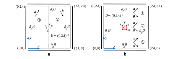
Figure 12: Hydraulically induced crack driven by fluid volume injection. (a) Example 3. Layered transversely isotropic poroelastic material, and (b) Example 4. layered orthotropy anisotropic poroelastic material.

4.3.1 Estimation of the penalty parameter

In this example, we first assume that the penalty parameter is a random field. Therefore, we strive to study the effect of its randomness on each element.

The Karhunen-Loéve expansion (KLE) expansion technique is a useful computational method used to reduce the dimensionality of the random field. Here the field $\Lambda$ indicates the penalty parameter (here $\beta_{a}$ while $\beta_{g}=0$ is fixed) and can be decomposed by its mean value and variation. Denoting the probability density function $\mathbb{P}$ and the random variable $\omega\in\Omega$ belongs the probability space $\Omega$, the covariance function has the form

$$\operatorname{Cov}_{\Lambda}({\mathbf{x}},{\mathbf{y}})=\int_{\Omega}\left(\Lambda({\mathbf{x}},\omega)-\Lambda({\mathbf{x}})\right)\left(\Lambda({\mathbf{y}},\omega)-\Lambda({\mathbf{y}})\right)\,\text{d}\mathbb{P}(\omega).$$ (58)

Therefore, the the KL-expansion reads

$$\Lambda({\mathbf{x}},\omega)=\bar{\Lambda}({\mathbf{x}})+\sum_{i=1}^{\infty}\sqrt{\psi_{i}}k_{i}({\mathbf{x}})\xi_{i}(\omega).$$ (59)

The first term indicates the expectation, $k_{i}$ are the orthogonal eigenfunctions, $\psi_{i}$ are the corresponding eigenvalues of the eigenvalue problem

$$\int_{\mathcal{B}}\text{Cov}_{\Lambda}({\mathbf{x}},{\mathbf{y}})k_{i}({\mathbf{y}})~{}d{\mathbf{y}}=\psi_{i}k_{i}({\mathbf{x}}),$$ (60)

and the $\{\xi_{i}(\omega)\}$ are mutually uncorrelated random variables satisfy the following condition

$$\mathbb{E}[\xi_{i}]=0,\hskip 10.00002pt\mathbb{E}[\xi_{i}\xi_{j}]=\delta_{ij}.$$ (61)

Also $\mathbb{E}$ denotes the expected value of the random variables, and $\delta_{ij}$ denotes the Kronecker product. For the Gaussian random field, we use a Gaussian covariance kernel defined by

$$\operatorname{Cov}_{\Lambda}({\mathbf{x}},{\mathbf{y}})=\sigma^{2}\exp\left(-\frac{(x_{1}-y_{1})^{2}}{\zeta_{1}}-\frac{(x_{2}-y_{2})^{2}}{\zeta_{2}}\right),$$ (62)

where $\zeta_{1}$, and $\zeta_{2}$ are the anisotropic correlation lengths and $\sigma$ is the standard deviation. The infinite series can be truncated to a finite series expansion (i.e., an $N_{\mathrm{KL}}$-term truncation) by

$$\Lambda({\mathbf{x}},\omega)=\bar{\Lambda}({\mathbf{x}})+\sum_{i=1}^{N_{{}_{\text{KL}}}}\sqrt{\psi_{i}}k_{i}({\mathbf{x}})\xi_{i}(\omega).$$ (63)

In order to define $N_{\mathrm{KL}}$, we use the following criterion

$$\frac{\sum_{i=1}^{N_{\mathrm{KL}}}\psi_{i}}{\sum_{i=1}^{\infty}\psi_{i}}=\mathrel{\mathop{\mathchar 58\relax}}\varphi,$$ (64)

to preserve the variance. In this work in order to decompose the random field (penalty parameters) we assume that it has the expectation of 55, the correlation lengths are $\zeta_{1}=0.1$, $\zeta_{2}=0.1$, the standard deviation is $\sigma=5$, and $\varphi=0.95$. The values of the random field in the elements is shown in Figure 13.

From now onward, due to dealing with the anisotropic solids, we follow the following parameter estimation procedure.

1. Propose $\theta^{*}\in$($\beta_{a},\,\beta_{g}$) according to the given distribution to determine the posterior density of the penalty parameters, i.e.,

   $$(\bar{\beta_{a}},\,\bar{\beta_{g}})=\text{DRAM}(\theta^{*},\upsilon),$$ (65)

   where other unknowns $(\upsilon=\{\mu,K,M,B,G_{c},\eta_{F}\})$ are according to the true values.

2. Then, use the extracted information from the estimated parameters to identify other unknown values, namely

   $$(\bar{\mu},\,\bar{K},\,\bar{M},\,\bar{B},\,\bar{G_{c}},\,\bar{\eta_{F}})=\text{DRAM}(\theta^{*},\bar{\beta_{a}},\,\bar{\beta_{g}}),$$ (66)

   where the candidates $\theta^{*}\in\{\mu,K,M,B,G_{c},\eta_{F}\}$ are proposed based on the given distribution.

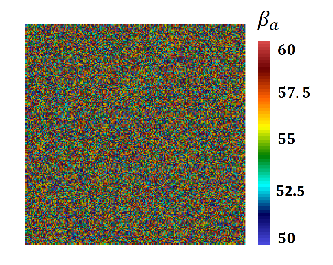
Figure 13: The values of the penalty-like parameter $\beta_{a}$ (prior density) on each element of the domain $\mathcal{B}$.

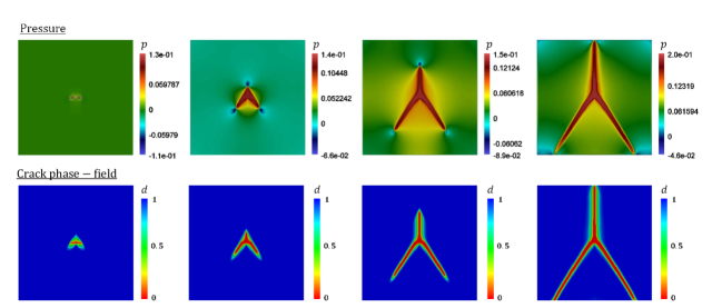
Figure 14: Example 3. Reference results of the hydraulically induced crack driven by the fluid volume injection for the layered orthotropy anisotropic poroelastic material. Evolution of the fluid pressure $p$ (first row) and crack phase-field $d$ (second row) for different deformation stages up to final failure at $t=0.1,\,5.1,\,20.1,\,44.5$ seconds.

Next, we start our analysis by illustrating the computed reference results for different fluid injection time up to final failure related to Figure 12(a). The fluid pressure $p$ (first row) and crack phase-field $d$ (second row) evolutions are demonstrated in Figure 14 for four-time steps, i.e., $t=0.1,\,10,\,40,\,80.2$ seconds. The crack initiates at the notch-tips due to fluid pressure increase. The crack profile at first time step (i.e. $t=0.1$ second), evidently intend to the preferential fiber direction within each layer (see diffusivity area in Figure 14, second row). Afterward, the crack phase-field propagates toward fiber directions and in some certain time ($t=10$ second), secondary crack initiates through the middle point of the notch induced by fluid injection and then propagates through the interface between two layers. That is an interesting observation (and it is typical for the interface problem) which is shown in Figure 14 at $t=40$ second. Primary and secondary crack propagates in three directions towards the boundaries. Same as before, in the fractured zone, $p$ is almost constant due to the increased permeability inside the crack while low fluid pressure in the surrounding is observed. Another impacting factor that should be noted, the highest pressure is aligned with the highest strength direction of the material at each layer, see Figure 14, the first row.

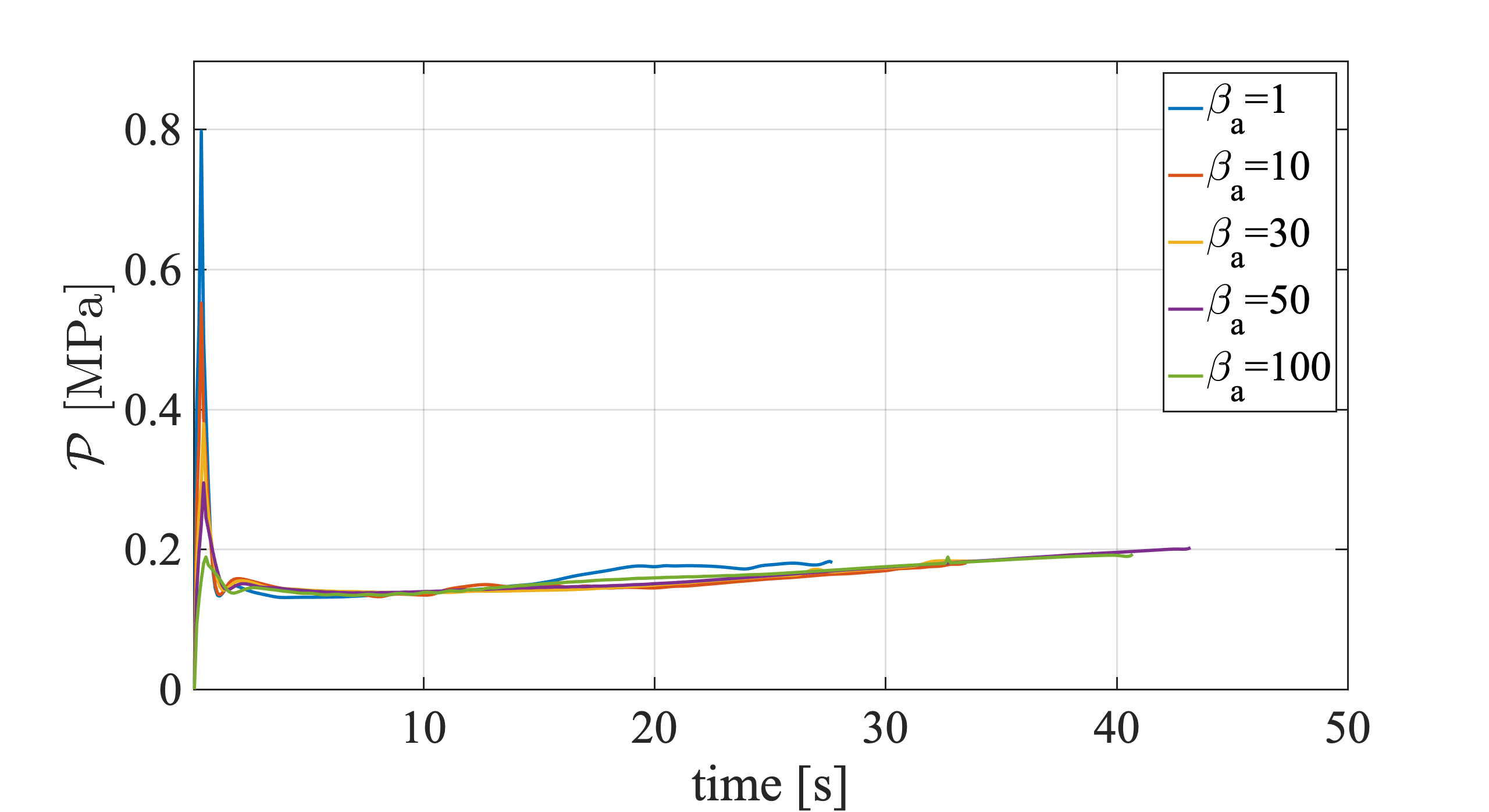
Figure 15: Example 3. The effect of penalty parameter on $\mathcal{P}$.

The effect of different $\beta_{a}$ on $\mathcal{P}$ is shown in Figure 15. As we already mentioned the penalty parameter is assumed a random field, and the KL-expansion used to determine the parameter in the elements. We extract the information to estimate the penalty parameter, where the probability density is shown in Figure 16.

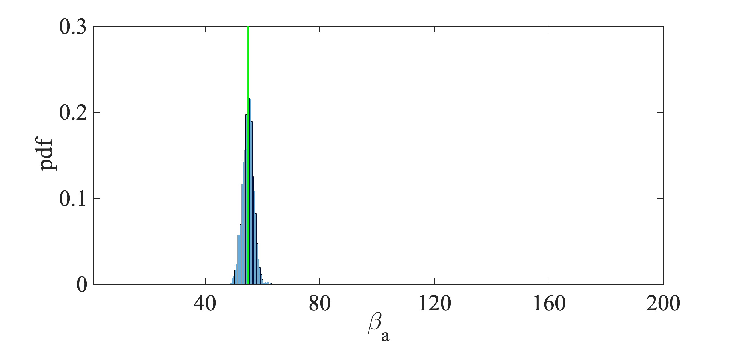
Figure 16: Example 3. The probability density of the penalty parameter.

Now, we strive to determine the desired values (using the determined $\beta_{a}$). The effect of the different values of the parameters on $\mathcal{P}$ is depicted in Figure 17 and the obtained posterior densities are shown in Figure 18. The different ending point of the curves is due to the impact of the parameters on the crack propagation (reaching the boundary). Then, we compare the estimated knowledge from the posterior with prior value (see Figure 19). Using the posterior information we can estimate the peak point and the pressure ending point precisely.

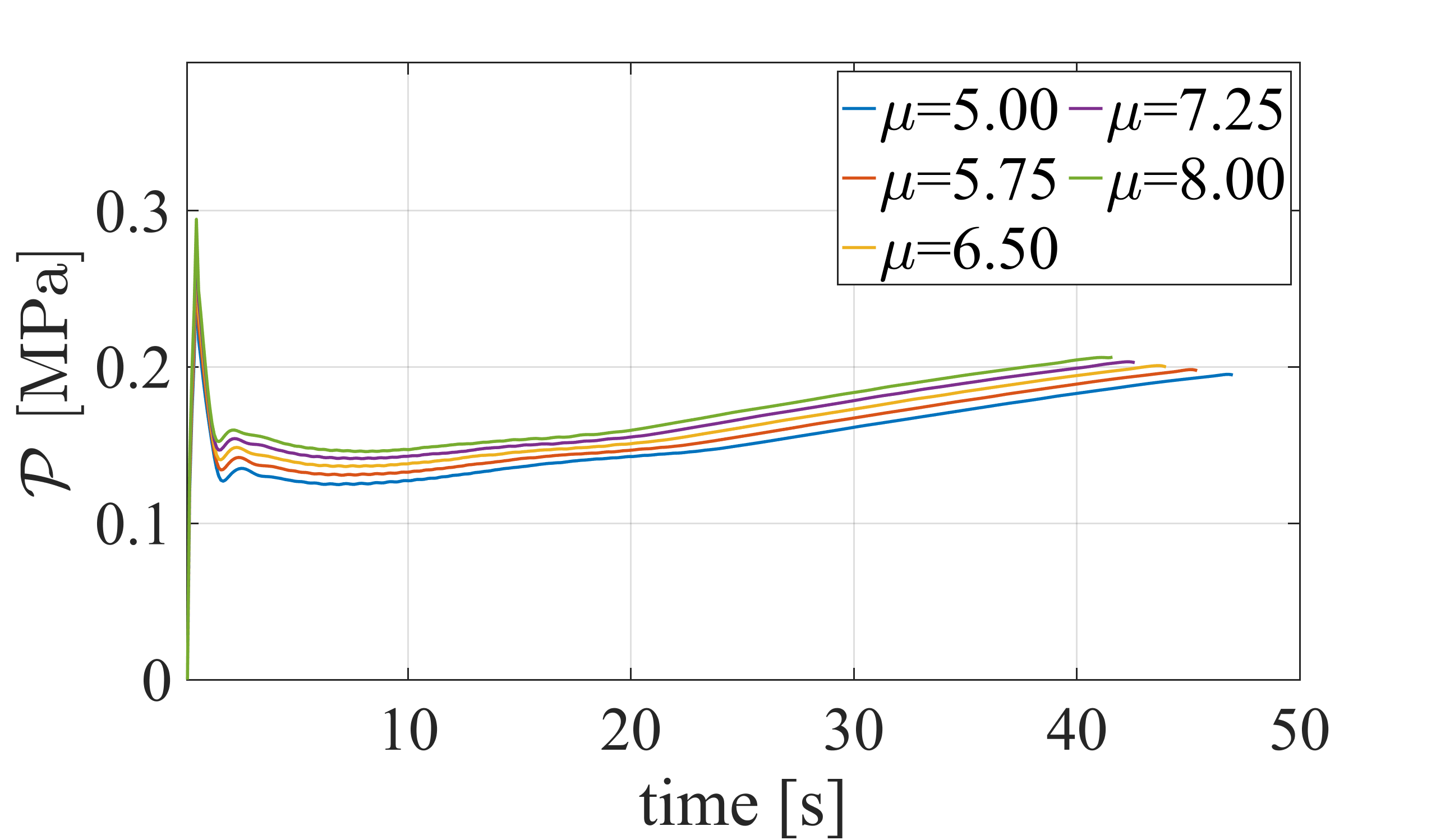
(a)

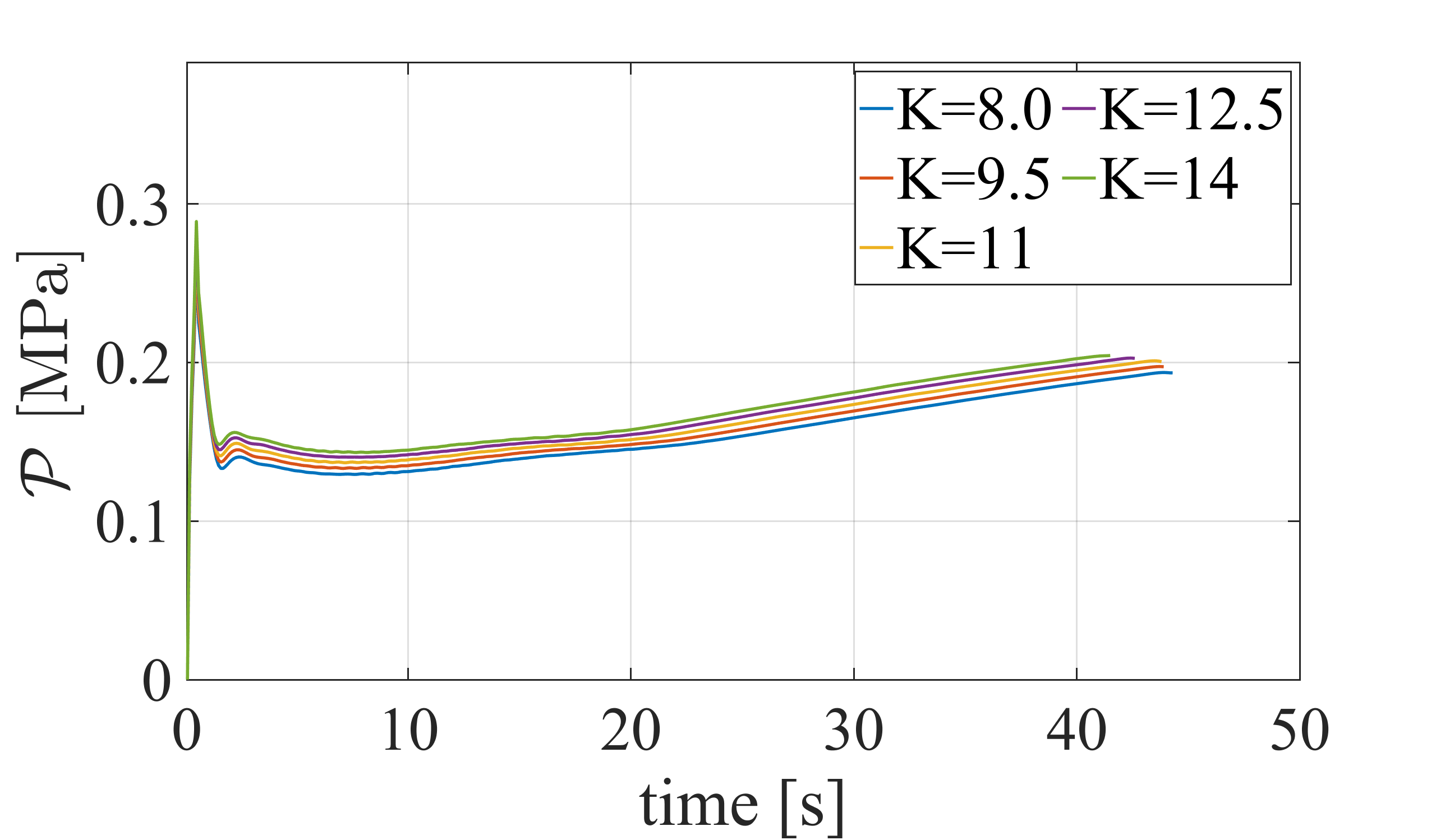
(b)

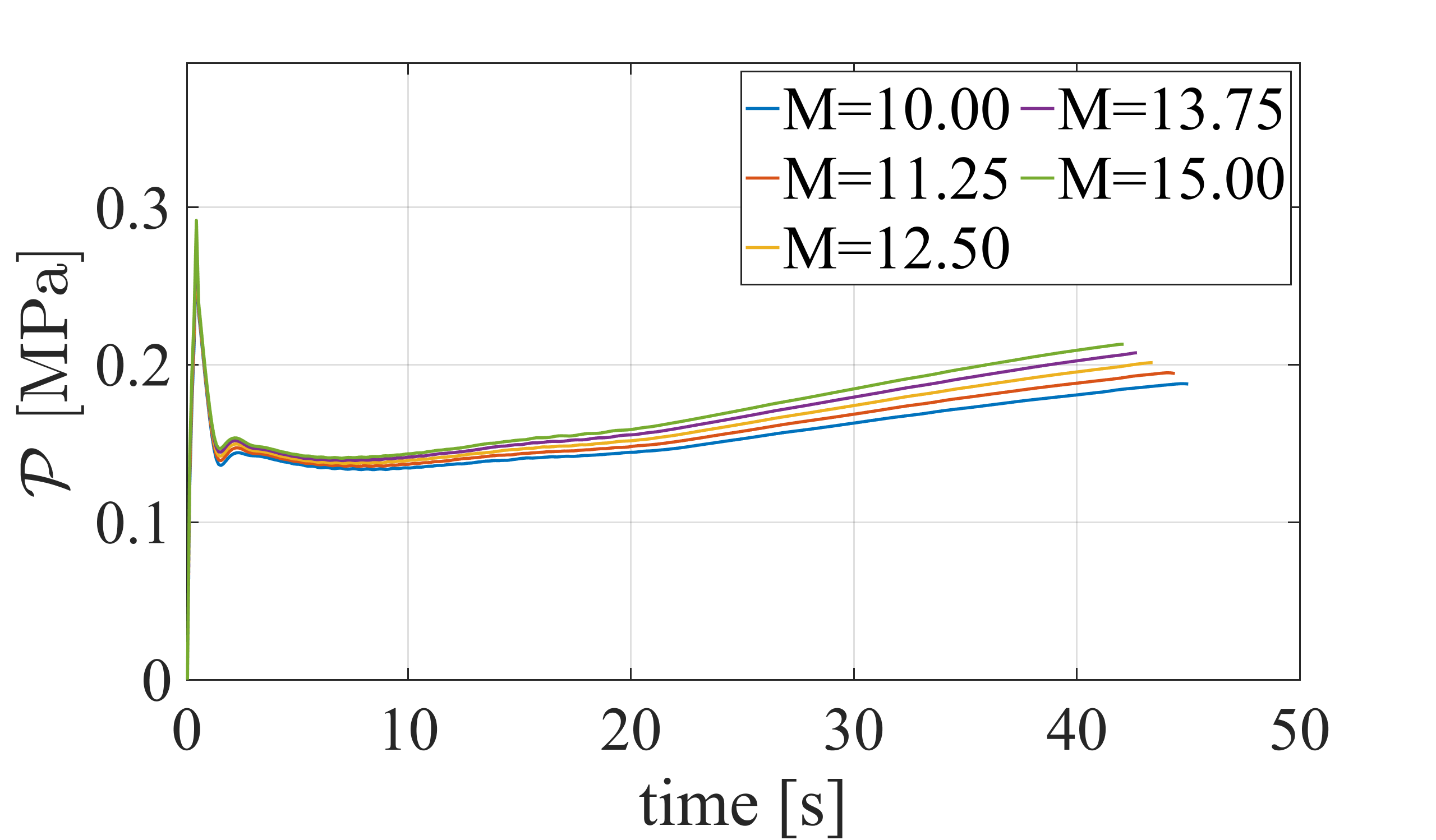
(c)

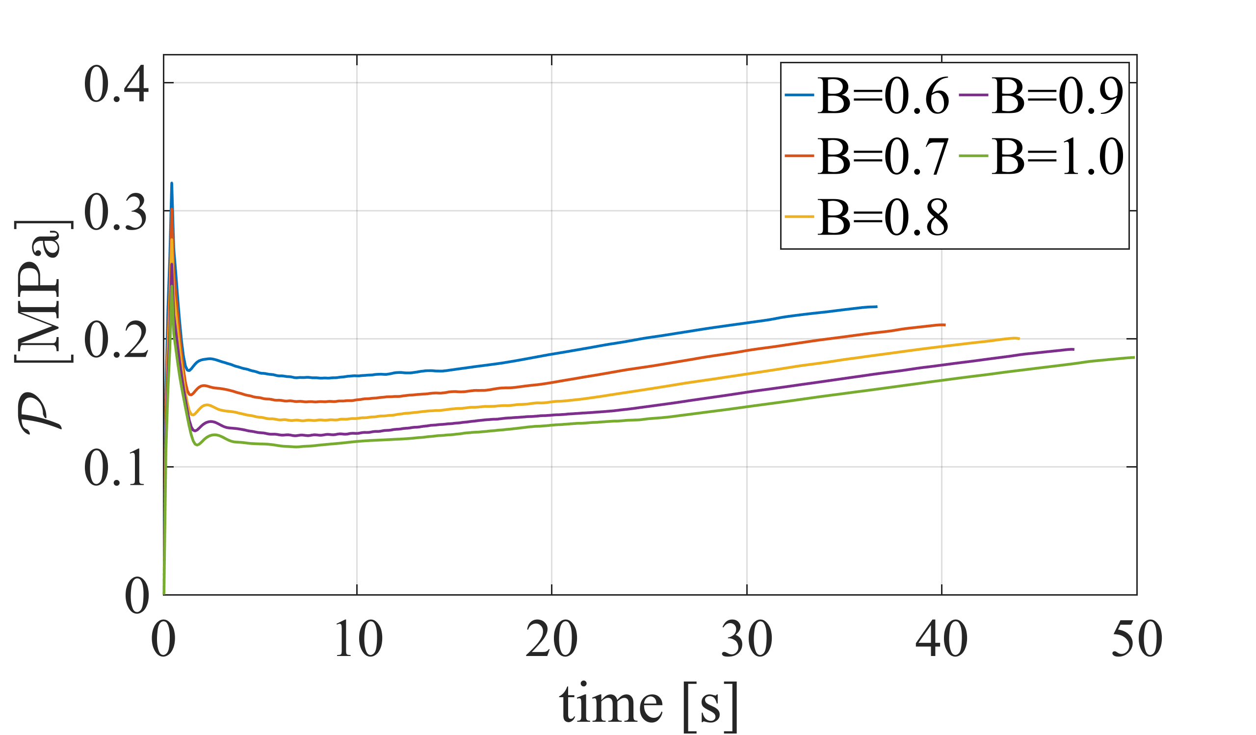
(d)

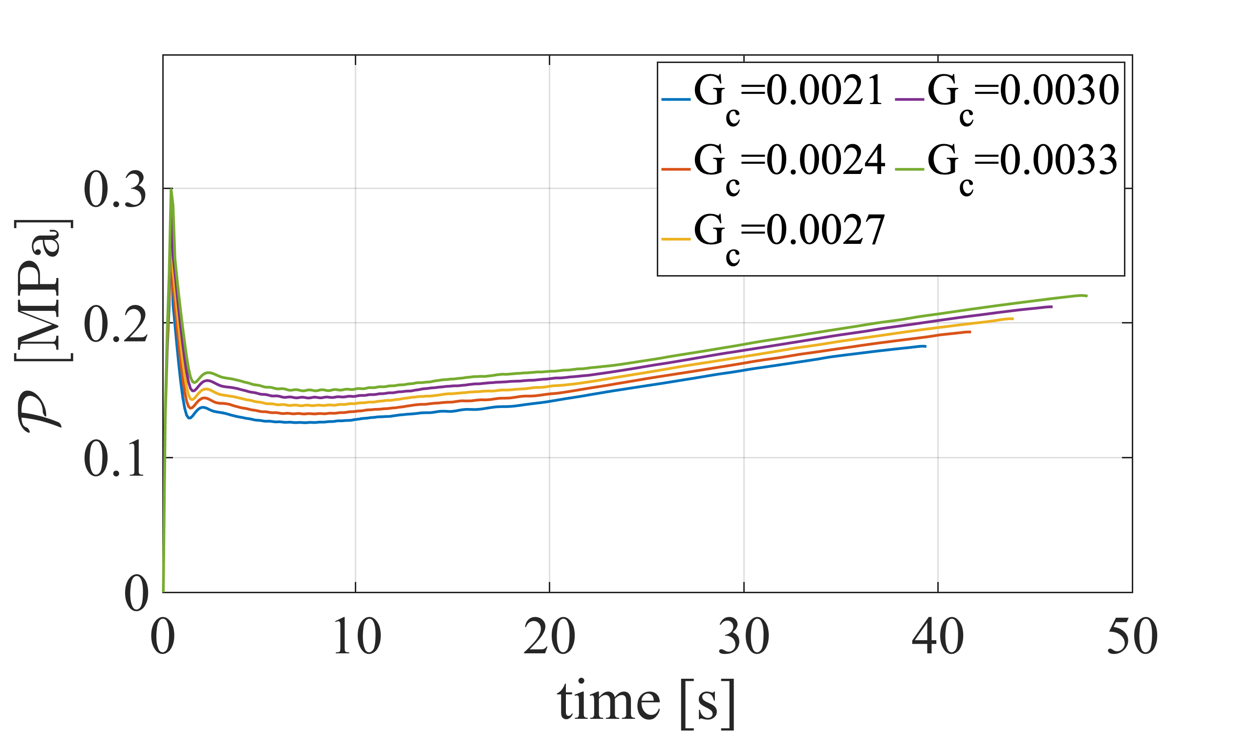
(e)

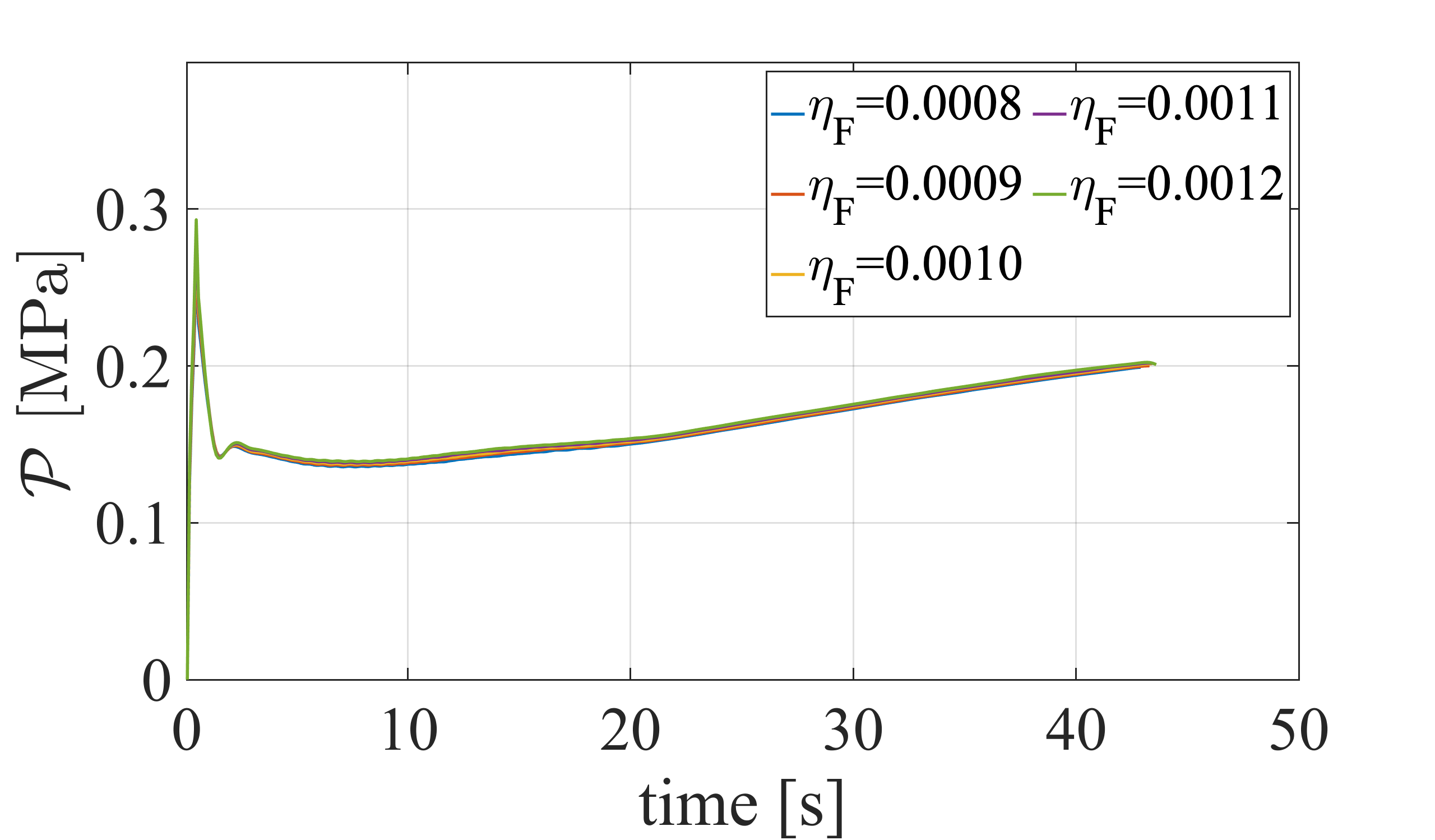
(f)

Figure 17: Example 3. The maximum pressure value $\mathcal{P}$ for different values of $\mu$, $K$, $M$, $B$, $G_{c}$, and $\eta_{F}$.

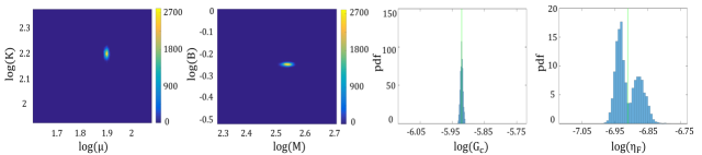
Figure 18: Example 3. From left to right: the posterior density of the mechanical parameters, Biot’s coefficients/modulus, $G_{c}$, and $\eta_{F}$. The green lines are the mean values.

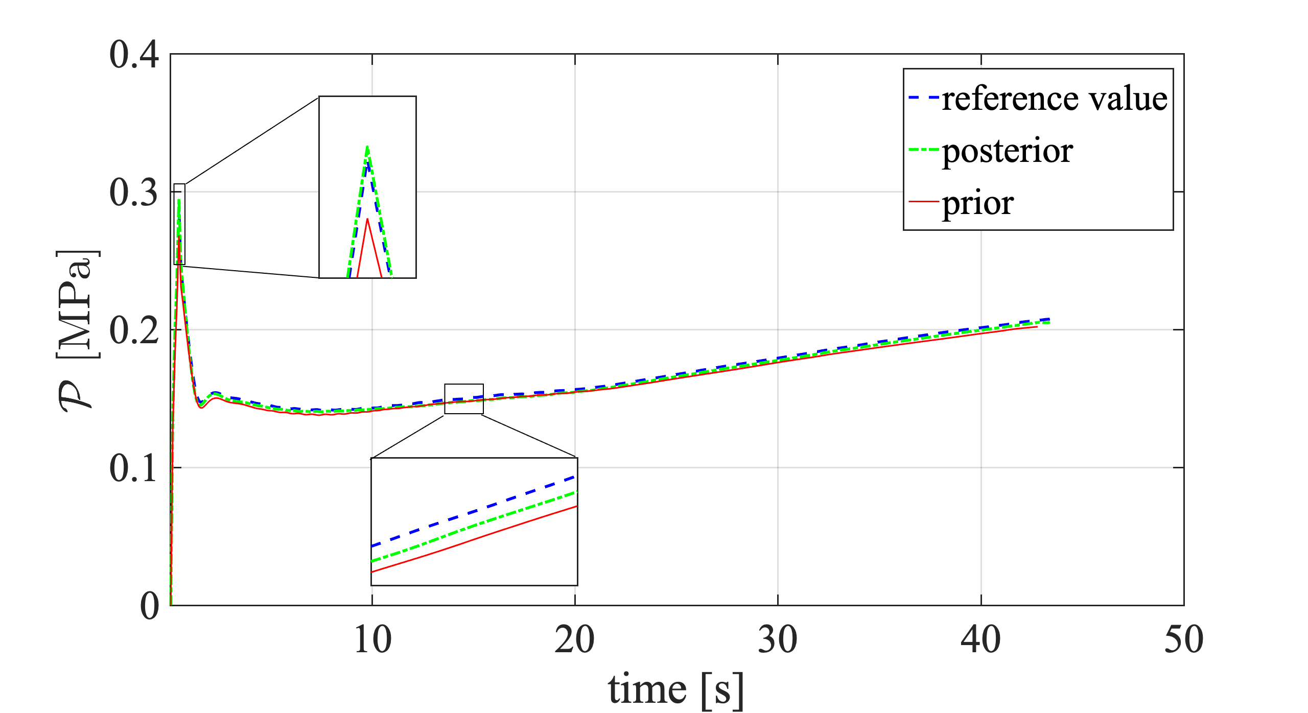
Figure 19: Example 3. A comparison between the maximum pressure (during the injection time) with prior values (red line) and the posterior values (green line). The reference diagram is depicted with a blue line.

4.4 Example 4: Orthotropy anisotropic fracture for a poroelastic layered material induced by fluid volume injection

The last numerical test is concerned with orthotropic anisotropic poroelastic materials with two families of fibers induced by the fluid volume injection. The layered boundary value problem is given in Figure 12b. The material properties are used the same as before. A constant fluid flow of $\bar{f}=0.004\;m^{2}/s$ is injected in $\mathcal{C}$ until failure for $T=13$ second with time step $\Delta t=0.1$ second during the simulation.

Here, the domain is divided identically into three horizontal layers (see Figure 12b) with a thickness of $2A/3=26.66~{}m$. Each layer of the poroelastic material is reinforced with two orthogonal unidirectional fibers embedded in the matrix, namely $\bm{a}$ and $\bm{g}$. The preferential fiber direction in each layer of the laminate is given by the structural director $\bm{a}$ and ${\mathbf{g}}$ which is inclined by $\theta=+30^{\circ}$ and $\theta=-60^{\circ}$, respectively, with respect to the $x$-axis of a fixed Cartesian coordinate system. Here, penalty-like parameters act as a material parameter, hence families of fibers with higher penalty-like parameters respond stiffer, and hence anisotropic response is oriented in that direction. Specifically, we define the mismatched ratio between two families of fibers and denoted by $\xi$ which is given by

$$\xi^{i}\mathrel{\mathop{\mathchar 58\relax}}=\frac{\beta^{i}_{a}}{\beta^{i}_{g}}=\frac{\chi^{i}_{a}}{\chi^{i}_{g}},\quad\text{with}\quad i=(1,2,3).$$ (67)

Herein, $i$ refers to the layer number within the domain, see Figure 12b, with $(\beta_{a},\chi_{a})$ and $(\beta_{g},\chi_{g})$ are corresponding to the $\bm{a}$ and $\bm{g}$, respectively, see (30) and (46). Thus, if $\xi^{i}>1$ means $\bm{a}$ is stiffer than $\bm{g}$ then crack orientation is in direction parallel to $\bm{a}$. Otherwise, if $\xi^{i}<1$ means $\bm{g}$ is stiffer than $\bm{a}$ then crack orientation is in direction parallel to $\bm{g}$. To formulate the fracture process, the stiffer fiber is set with a larger value of the penalty-like parameter in the (30) and (46). Therefore, in the following, we considered four different cases.

• Case a. In the first case, we consider the isotropic hydraulic fracture and hence we fixed and set $\beta_{a}=\chi_{a}=\beta_{g}=\chi_{g}=0$ to recover isotropic formulation. The fluid pressure $p$ and the crack phase-field $d$ evolutions are shown in Figure 20 and 21 first row, respectively, for four-time steps, i.e., $t=0.1,\,5.1,\,10.1,\,12.2$ seconds. Here, the crack initiates at the notch-tips (where we have a singularity-like shape) due to fluid pressure increase. Then, it propagates about $45^{\circ}$ and in the very final stage, see Figure 21 the first row at $t=12.2$, we observed the crack branching near boundaries induced by the fluid injection.

• Case b. In this and the next two cases, for the first and third layers, we assume fiber $\bm{g}$ is stiffer than $\bm{a}$ while within the second layer $\bm{a}$ is stiffer than $\bm{g}$. Hence, we set $\beta^{1}_{g}=\beta^{2}_{a}=\beta^{3}_{g}=10$ and $\beta^{1}_{a}=\beta^{2}_{g}=\beta^{3}_{a}=0.5$. The same values are also holds for the ($\chi^{i}_{a}$,$\chi^{i}_{g}$) with $i=(1,2,3)$. Table 3 summarizes penalty parameters and the mismatch ratio for each layer. The fluid pressure $p$ and crack phase-field $d$ evolutions are shown in Figure 20 and 21 second row, respectively, for four-time steps, i.e., $t=0.1,\,3.1,\,5.1,\,11.4$ seconds. Here, the crack initiates at the notch-tips due to fluid pressure increase. The crack profile at first time step (i.e. $t=0.1$ second), propagate toward the preferential fiber direction $\beta_{a}$ in the second layer. Afterwards, the crack phase-field initiates and then propagates along the interface between layers 2 and 1 and, accordingly, layer 2 and 3, see Figure 21, second row. This crack profile occurs mainly because the material is not very stiff in the preferential direction such that crack propagates toward the fibers. Thus, it continuous along the interface between two layers.

• Case c. In this case, we set $\beta^{1}_{g}=\beta^{2}_{a}=\beta^{3}_{g}=50$ and $\beta^{1}_{a}=\beta^{2}_{g}=\beta^{3}_{a}=2.5$. The same values are also holds for the ($\chi^{i}_{a}$,$\chi^{i}_{g}$) with $i=(1,2,3)$. By means of Table 3, in layer 2 where $\xi^{i}>1$, crack propagate in a direction of $\bm{a}$, otherwise $\bm{g}$, e.g. layers 1 and 3. The fluid pressure $p$ and crack phase-field $d$ evolutions are shown in Figure 20 and 21 third row, respectively, for four-time steps, i.e., $t=0.1,\,3.1,\,5.1,\,12$ seconds. Here, the crack initiates at the notch-tips due to fluid pressure increase. The crack profile at first time step (i.e. $t=0.1$ second), evidently intend to the preferential fiber direction within each layer (see diffusivity area in Figure 21, third row). Afterwards, the crack phase-field propagates toward fiber directions which is inclined under $\theta=+30^{\circ}$, because we have a situation $\xi>1$, meaning that the stiffer response is observed in ${\mathbf{a}}$ orientation of the poroelastic material ($t=3.1$ second). In some certain time ($t=5.1$ second), the crack direction is changed toward ${\mathbf{g}}$ ($\theta=-60^{\circ}$) since $\xi<1$. A secondary crack initiates along the interface between two layers which is depicted in Figure 21 at $t=12$ second. Additionally, it can be grasped the highest pressure is aligned with the highest strength direction of the material at each layer, see Figure 20, the third row.

• Case d. Here, we set $\beta^{1}_{g}=\beta^{2}_{a}=\beta^{3}_{g}=200$ and $\beta^{1}_{a}=\beta^{2}_{g}=\beta^{3}_{a}=10$. The same values are also holds for the ($\chi^{i}_{a}$,$\chi^{i}_{g}$) with $i=(1,2,3)$. The fluid pressure $p$ and crack phase-field $d$ evolutions are shown in Figure 20 and 21 last row, respectively, for four-time steps, i.e., $t=0.1,\,3.1,\,5.1,\,10.4$ seconds. The first important observation is that the crack surface, precisely, follows the mismatch ratio $\xi^{i}$ criteria indicated in Table 3. Another impacting factor that should be noted that the crack surface is very similar with Case c, except in this case, a secondary crack is not anymore observed. This is mainly because the material behaves much stiffer in each fiber direction compared to Case c.

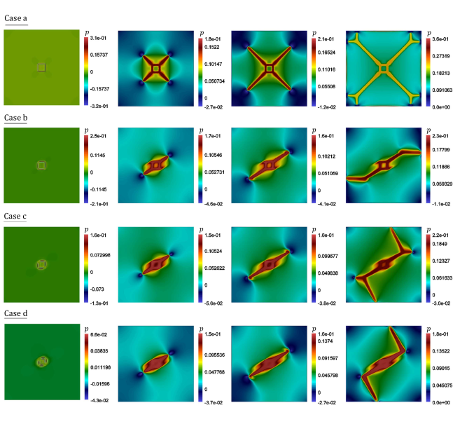
Figure 20: Example 4. Reference results of the hydraulically induced crack driven by the fluid volume injection for the layered anisotropic poroelastic material. Evolution of the fluid pressure $p$ for the Case a (first row) that is isotropic setting for different deformation stages up to final failure at $t=0.1,\,5.1,\,10.1,\,12.2$ seconds; Case b (second row) at $t=0.1,\,3.1,\,5.1,\,11.4$ seconds; Case c (third row) at $t=0.1,\,3.1,\,5.1,\,12$ seconds and Case d (fourth row) at $t=0.1,\,3.1,\,5.1,\,10.4$ seconds.

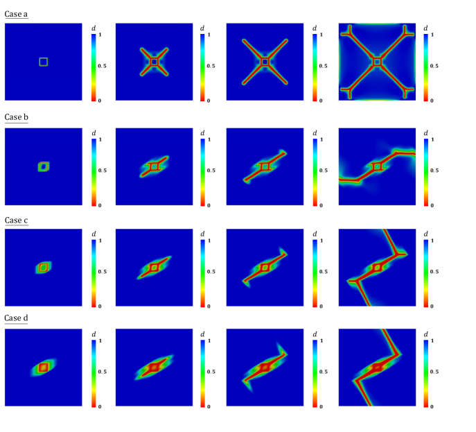
Figure 21: Example 4. Reference results of the hydraulically induced crack driven by the fluid volume injection for the layered anisotropic poroelastic material. Evolution of the crack phase-field $d$ for the Case a (first row) that is isotropic setting for different deformation stages up to final failure at $t=0.1,\,5.1,\,10.1,\,12.2$ seconds; Case b (second row) at $t=0.1,\,3.1,\,5.1,\,11.4$ seconds; Case c (third row) at $t=0.1,\,3.1,\,5.1,\,12$ seconds and Case d (fourth row) at $t=0.1,\,3.1,\,5.1,\,10.4$ seconds.

$(\beta_{a},\beta_{g},\xi)$	$layer\;1$	$layer\;2$	$layer\;3$
Case a	(0, 0, –)	(0, 0, –)	(0, 0, –)
Case b	(0.5, 10, 0.05)	(10, 0.5, 20)	(0.5, 10, 0.05)
Case c	(2.5, 50, 0.05)	(50, 2.5, 20)	(2.5, 50, 0.05)
Case d	(10, 200, 0.05)	(200, 10, 20)	(10, 200, 0.05)

Table 3: Example 4. The mismatched ratio $\xi$ between two families of fibers $(\bm{a},\bm{g})$. Large value for $\xi>1$, e.g. $\xi=20$, results stiffer response in direction of structural director $\bm{a}$ otherwise $\bm{g}$.

Next, in order to investigate the accuracy of the Bayesian framework, for this example, we consider Case b and also Case d. The first main goal is to identify the penalty parameter in all layers. As we already mentioned, in each region, different $\beta_{a}$ and $\beta_{g}$ are employed where the prior densities and the true values are shown in Table LABEL:prior. Figure 22 shows the joint probability density of both penalty parameters. As shown for both parameters a narrow distribution is obtained.

Using the estimated penalty parameters (the posterior densities), we present the effect of the unknown parameters on $\mathcal{P}$ in Figure 23 and the posterior densities (joint/marginal) are depicted in Figure 24. Finally, we used the obtained information to compared the posterior and prior densities as shown in Figure 25(a).

We use the same Bayesian framework for Case d and strive to estimate the penalty parameters. Again, the prior densities and the true values are shown in Table LABEL:prior. The effect of the parameters in different layers on $\bm{u}$ and $p$ can be observed in the last line of Figure 20 and Figure 21, respectively. Figure 26 shows the posterior density for the three-layer, were compared to Case b a wider distribution is obtained. Using the extracted mean values (of the posterior density), we solve the system of equations to study the effect of the penalty parameter on the pressure curve as shown in Figure 26. We consider which parameter is more influential on the pressure pattern in Figure 27. Here, Biot’s coefficient is the most effective, although $\eta_{F}$ does not have a noticeable impression. We employ the Bayesian inversion to estimate the posterior density of the parameters and show the results in Figure 28. Finally, a comparison between the prior and posterior values with the reference observation is drawn in Figure 25(b).

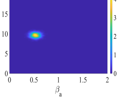
(a)

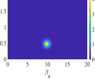
(b)

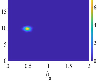
(c)

Figure 22: Example 4 (Case b). The joint probability density of the penalty parameters ($\beta_{a}$ and $\beta_{g}$) in layer 1 (left), layer 2 (middle), and layer 3 (right).

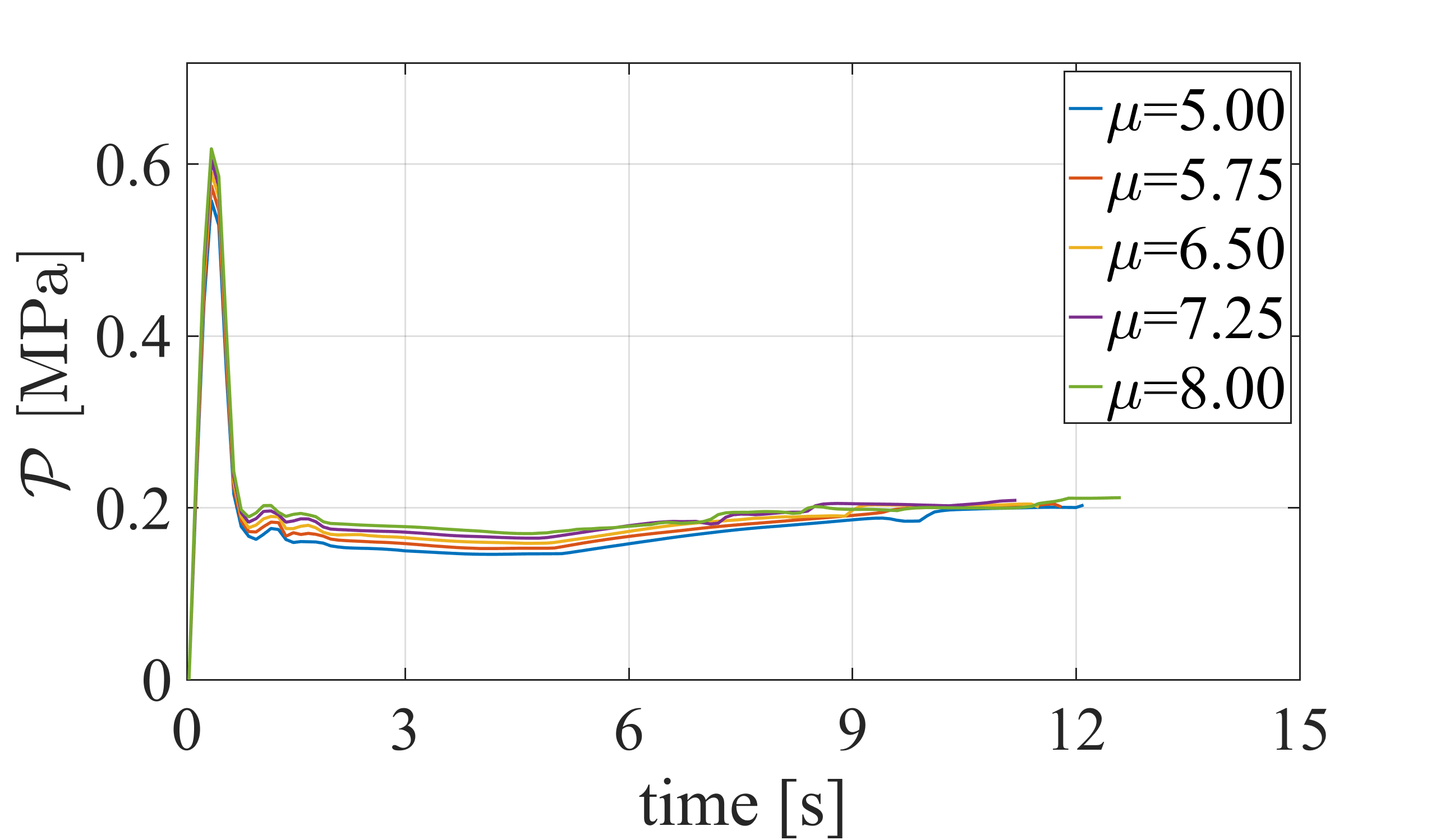
(a)

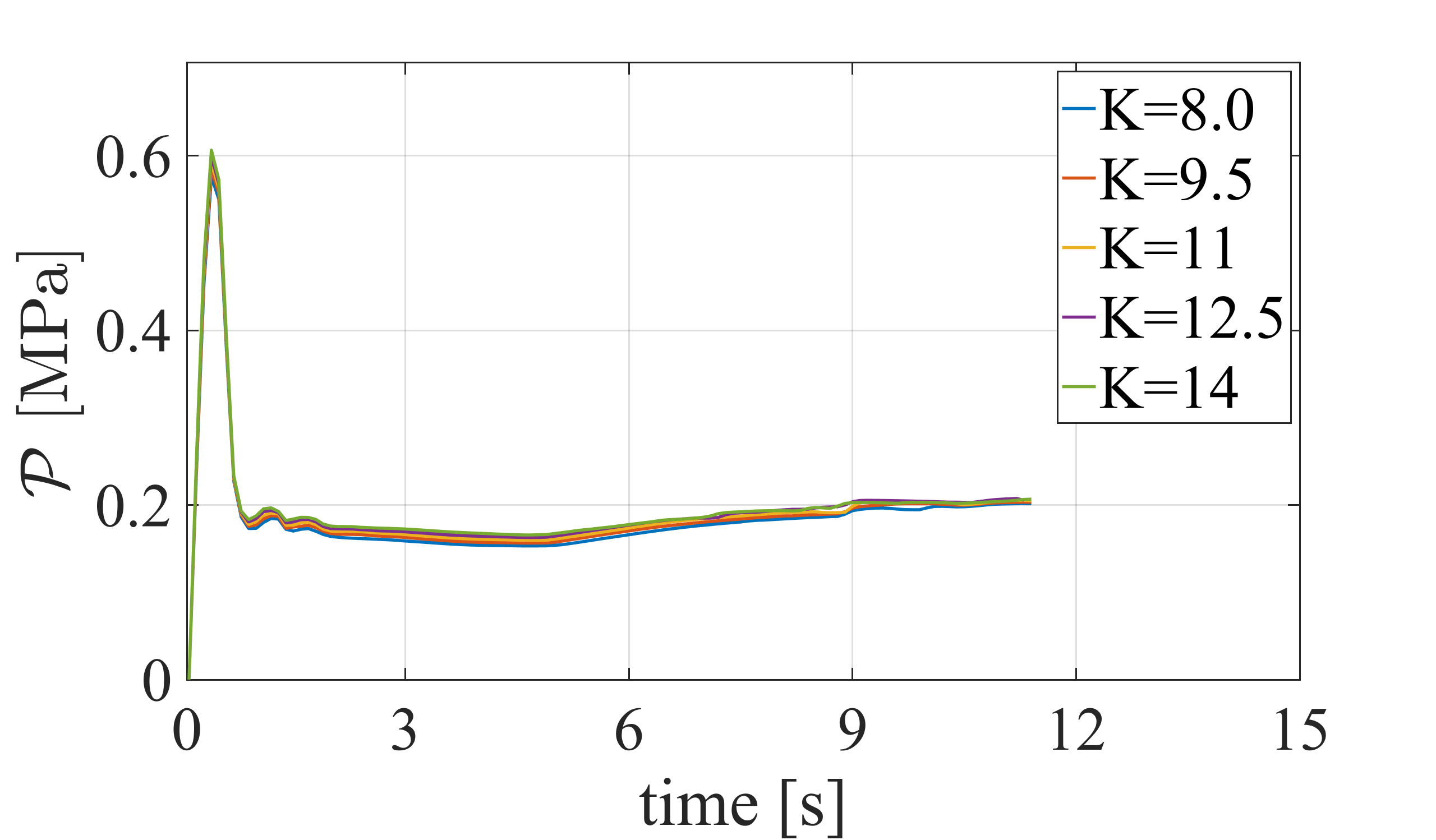
(b)

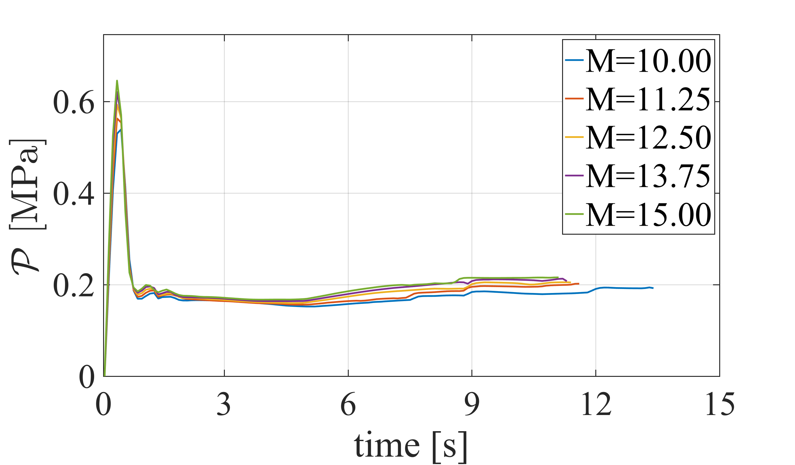
(c)

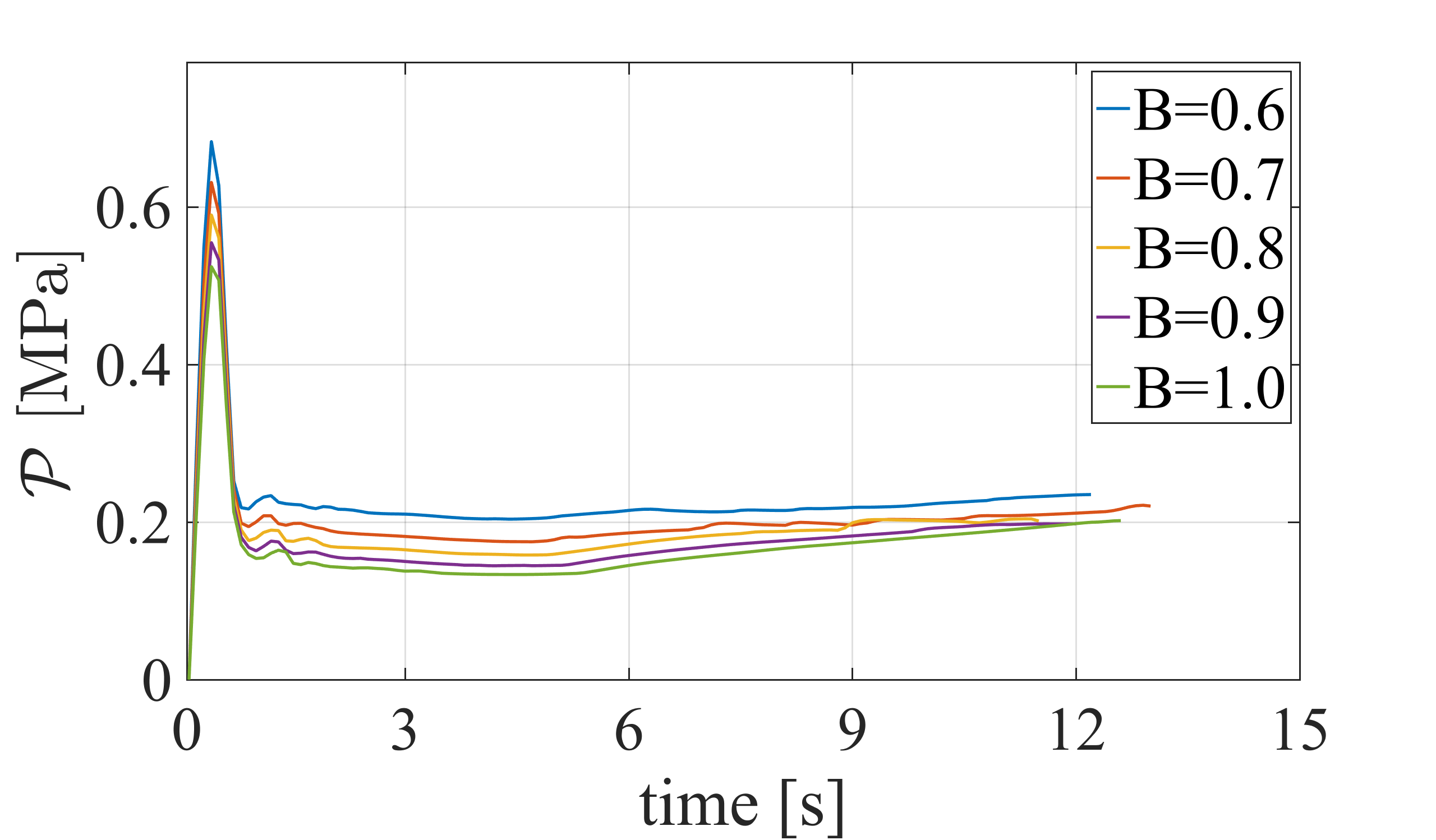
(d)

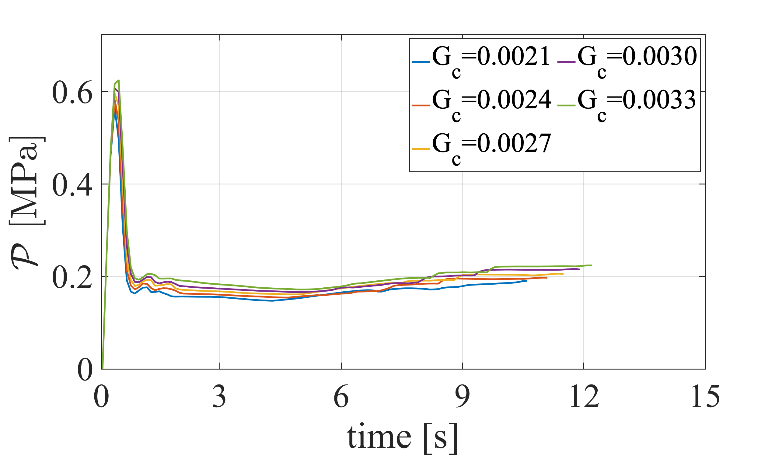
(e)

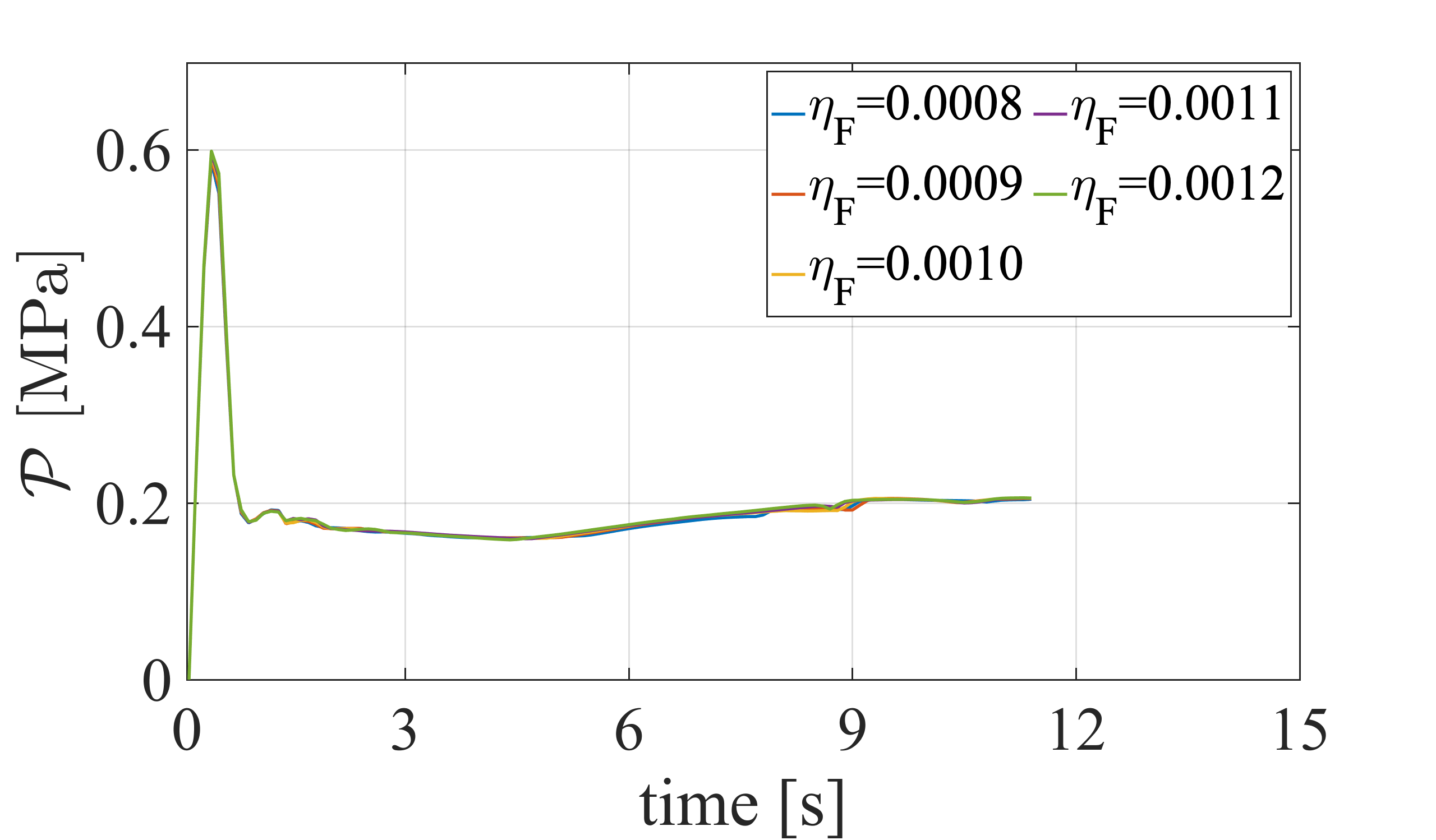
(f)

Figure 23: Example 4 (Case b). The maximum pressure value $\mathcal{P}$ for different values of $\mu$, $K$, $M$, $B$, $G_{c}$, and $\eta_{F}$.

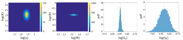
Figure 24: Example 4 (Case b). From left to right: the posterior density of the mechanical parameters, Biot’s coefficients/modulus, $G_{c}$, and $\eta_{F}$. The green lines are the mean values.

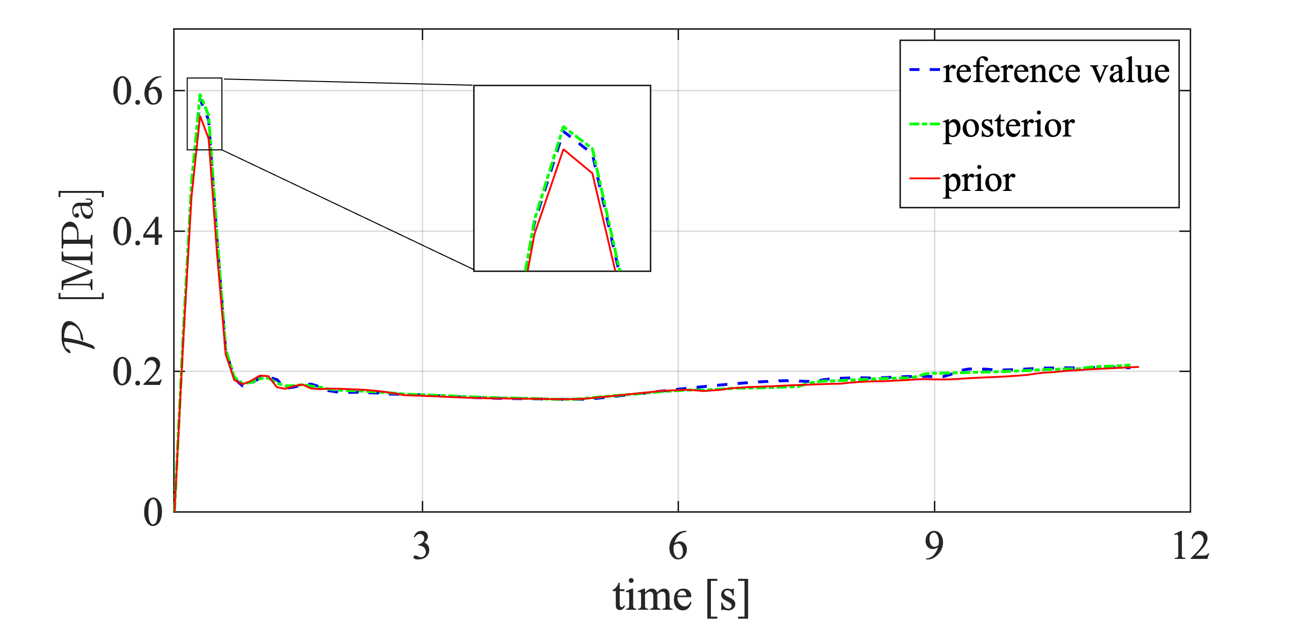
(a)

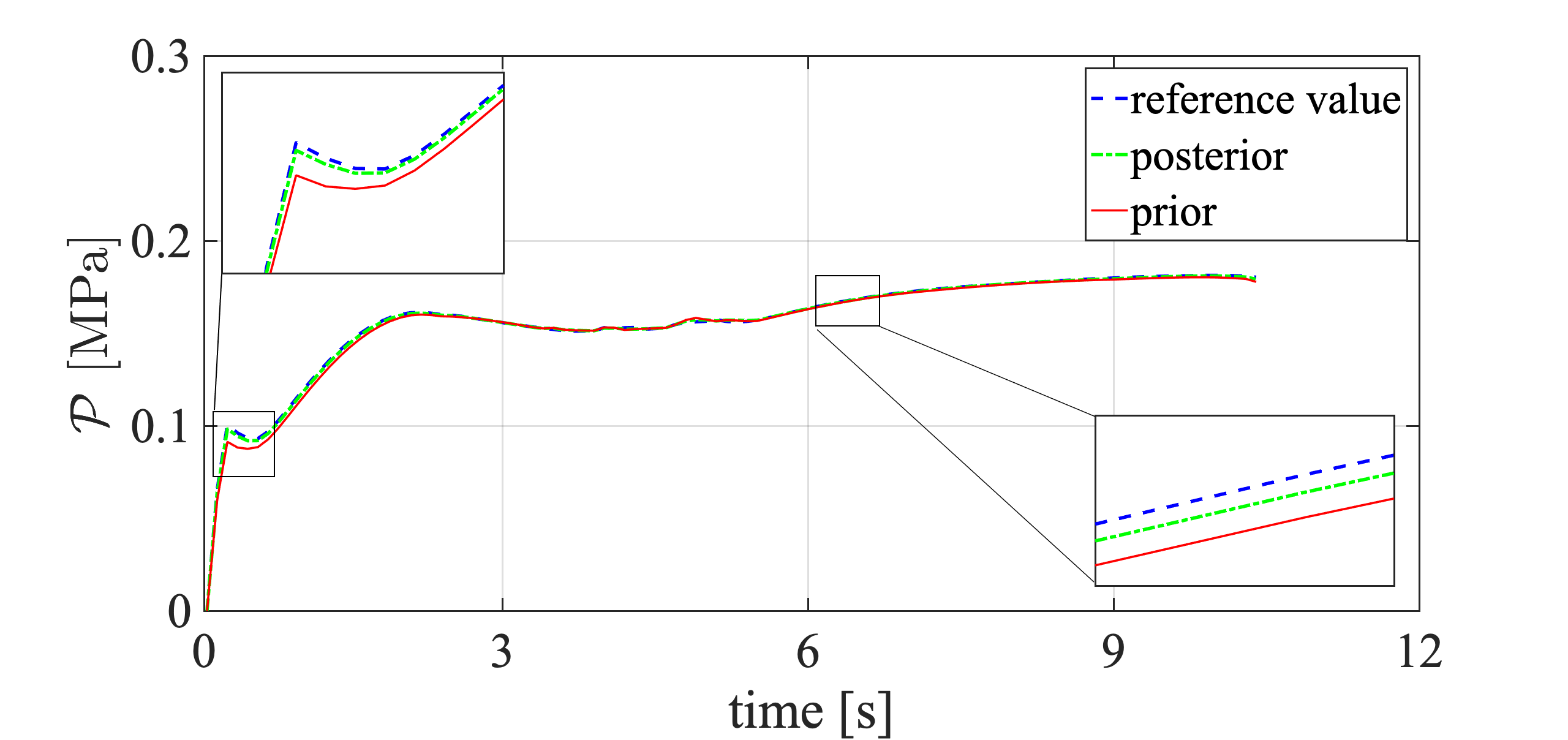
(b)

Figure 25: Example 4. A comparison between the maximum pressure (during the injection time) with prior values (red line), the posterior values (green line), and the reference diagram in Case b (left) and Case d (right).

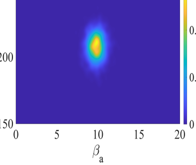
(a)

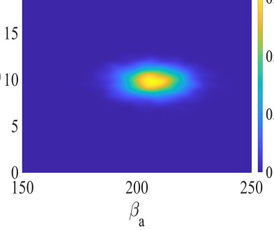
(b)

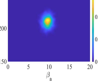
(c)

Figure 26: Example 4 (Case d). The joint probability density of the penalty parameters ($\beta_{a}$ and $\beta_{g}$) in layer 1 (left), layer 2 (middle), and layer 3 (right).

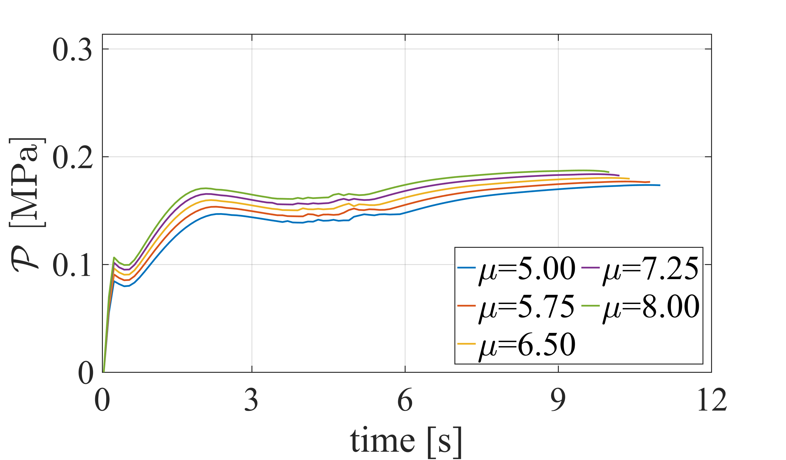
(a)

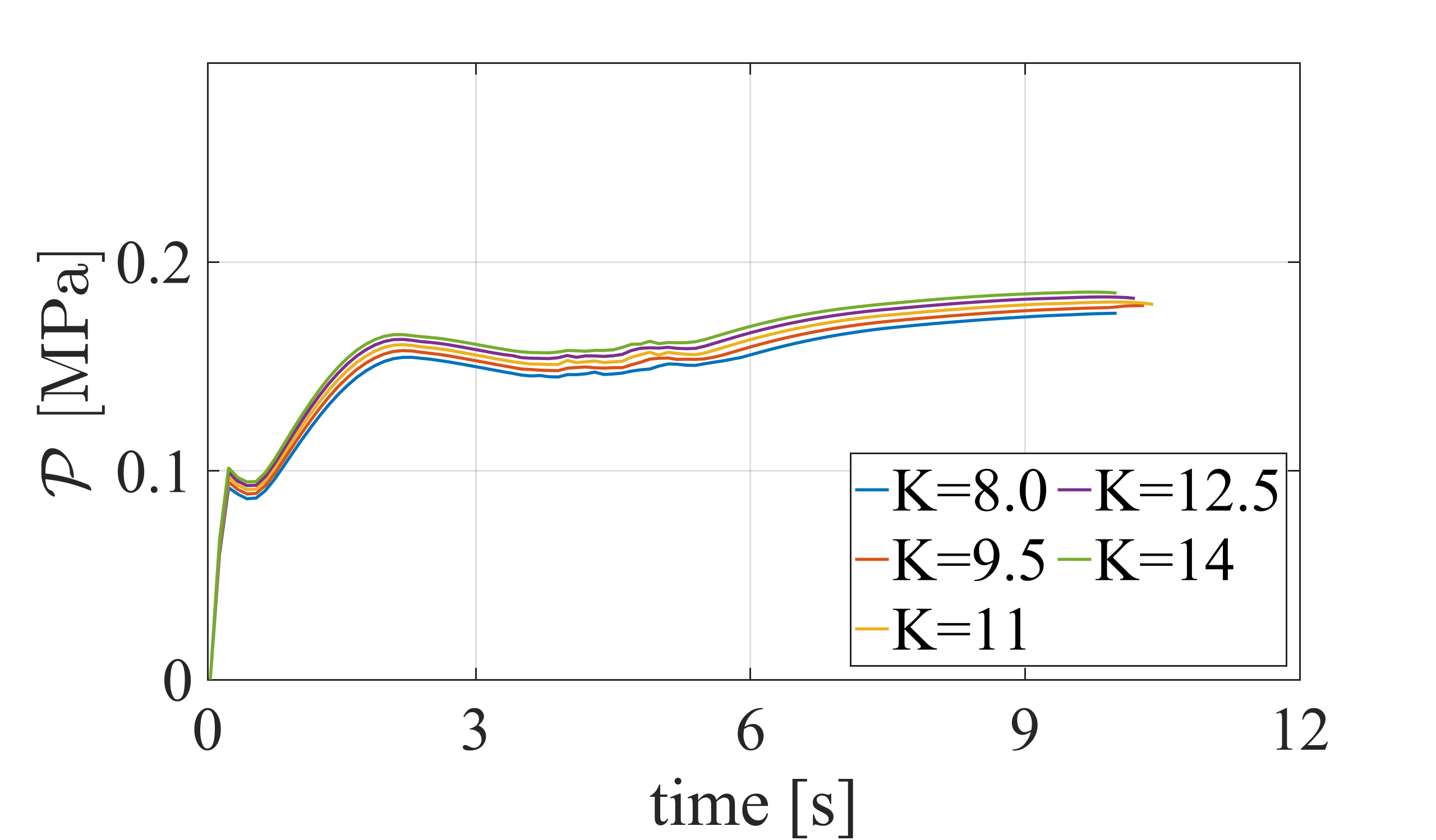
(b)

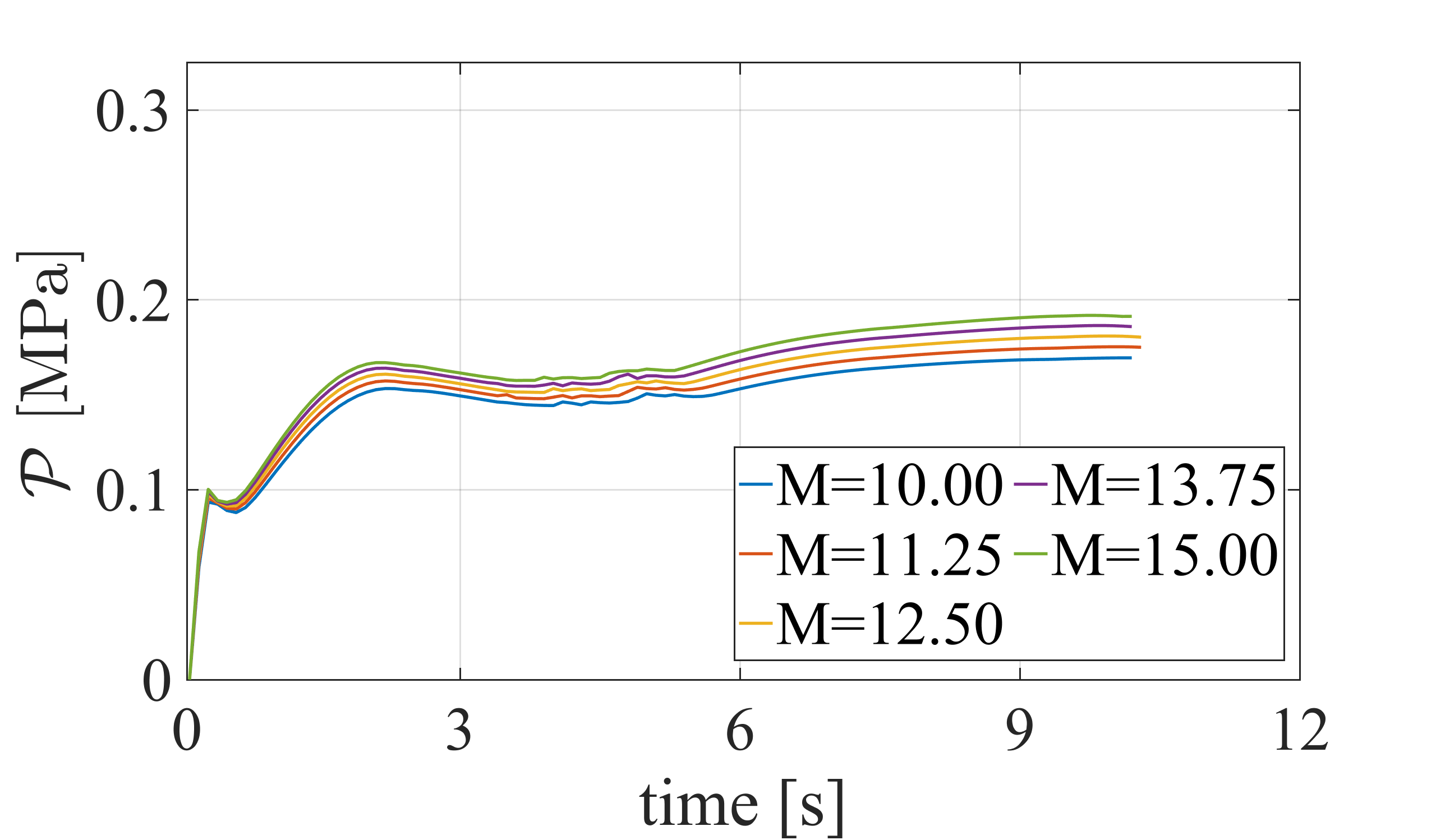
(c)

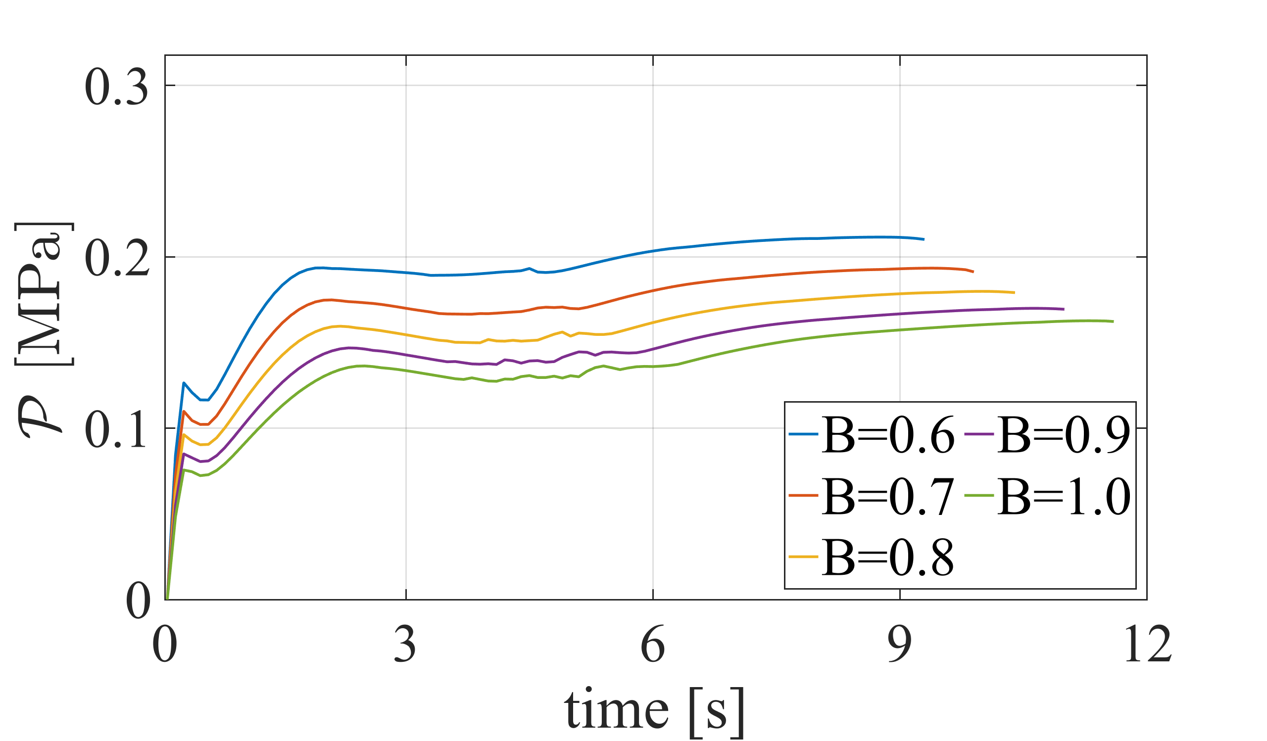
(d)

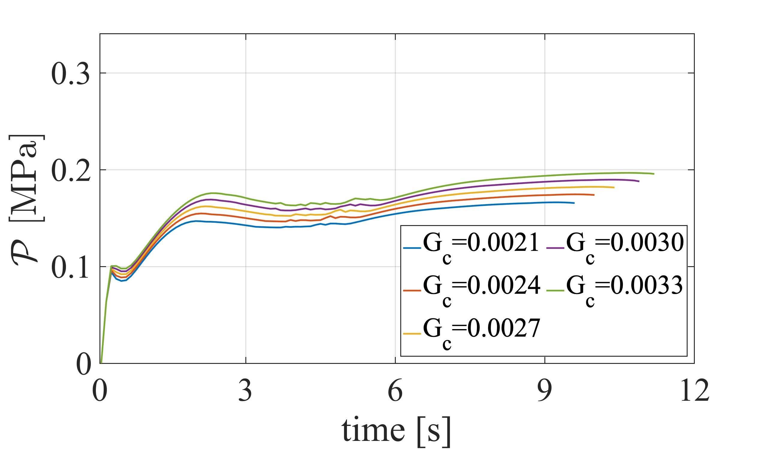
(e)

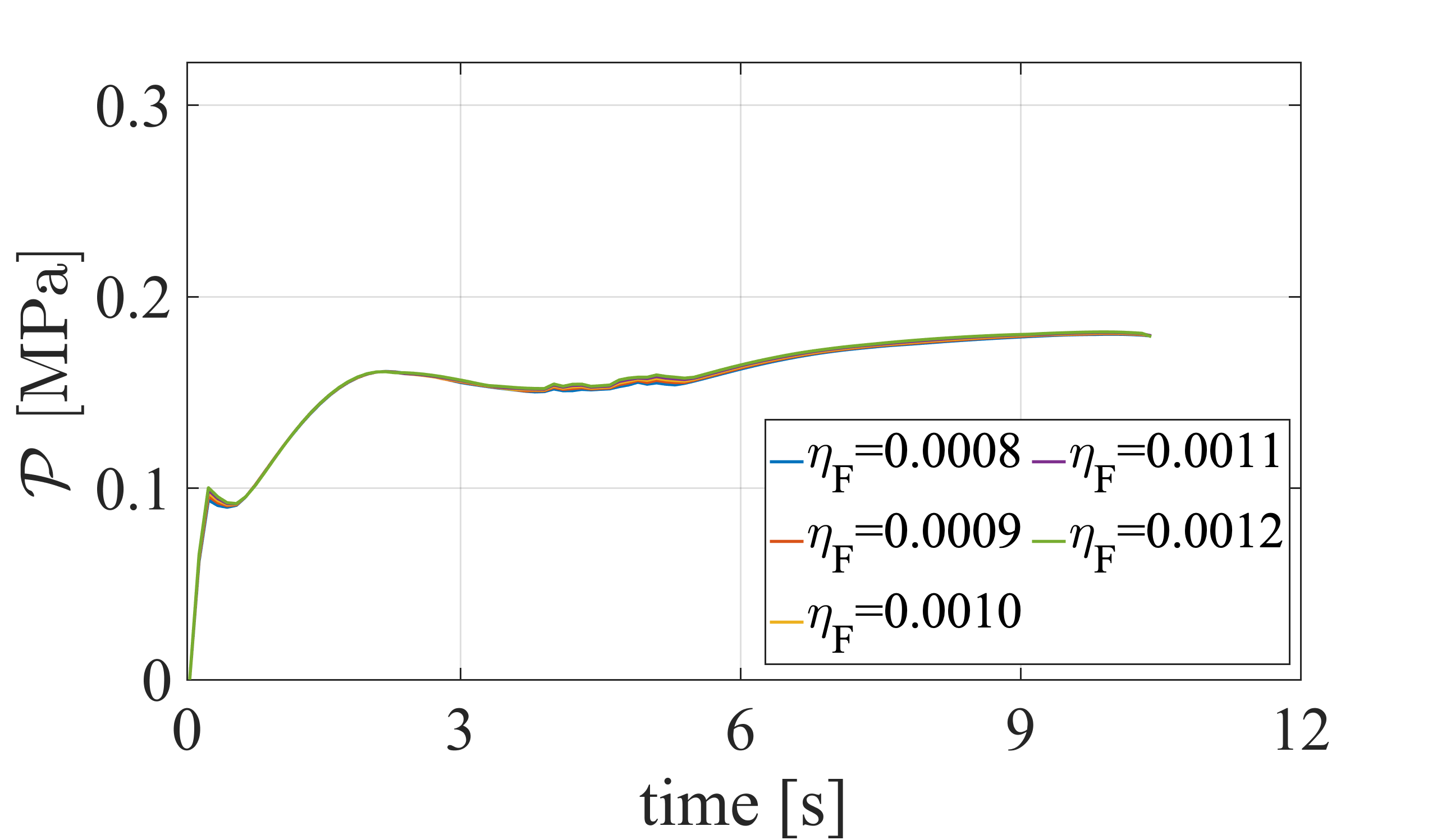
(f)

Figure 27: Example 4 (Case d). The maximum pressure value $\mathcal{P}$ for different values of $\mu$, $K$, $M$, $B$, $G_{c}$, and $\eta_{F}$.

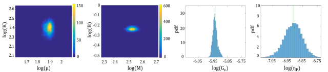
Figure 28: Example 4 (Case d). From left to right: the posterior density of the mechanical parameters, Biot’s coefficients/modulus, $G_{c}$, and $\eta_{F}$. The green lines are the mean values.

5 Conclusions

In this paper, we presented Bayesian inversion for parameter estimation in hydraulic phase-field modeling including transversely isotropic and orthotropy anisotropic fracture. Here, three specific model equations in the sense of pressure, displacement, and crack phase-field have been coupled. Direction-dependent responses due to the preferred fiber orientation in the poroelastic material are enforced via an additional anisotropic energy density function for both mechanical and phase-field equations. Furthermore, a new consistent additive split for the bulk anisotropic energy density function is introduced. More precisely, the crack driving state function for the poroelastic material was modeled such that the compression mode of the anisotropic energy is avoided to be degraded. Furthermore, we explained a fully monolithic solution for pressure and displacement, then a staggered approach has been employed for the crack phase-field equation.

Based on this forward model, we presented a probabilistic setting for hydraulic phase-field fracture. We adjusted the DRAM algorithm to determine various effective parameters in crack propagation. To this end, we used pressure during the fluid injection as the reference observation and strive to estimate six variables, including Lamé constants, Biot’s coefficient, Biot’s modulus, dynamic fluid viscosity, and Griffith’s energy release rate. The approach compared to usual MCMC techniques, e.g., Metropolis-Hastings showed more efficiency due to the proposal adaptation and the delayed rejection; therefore, a more reliable posterior density was obtained.

In total, we investigated four different examples including various test cases. In the last two examples, we applied our approach to transversely isotropic and orthotropic anisotropic poroelastic materials. In these cases, the uncertainty arising for the penalty-like parameters in addition to other unknowns is considered. Our findings showed that pressure evolves in the direction of the preferred fiber orientation. Additionally, the fracture profile is aligned with the highest strength direction of the poroelastic material. Penalty-like parameters for the anisotropic response, as well as other material properties, are well estimated through the proposed Bayesian inversion.

Appendix A. Finite Element Discretization

In the following, we deal with a multi-field problem to be solved with three-field unknowns represented by $({\mathbf{u}},p,d)$ to be solved from (49). Here, we aim to provide a detailed consistent linearization procedure within the finite element discretization setting. We use a Galerkin finite element method to discretize the equations with employing $H^{1}$-conforming bilinear (2D) elements, i.e., the ansatz and test space uses $Q_{1}^{c}$–finite elements. We refer interested readers to [72] for more details. Hence, the discrete spaces have the property ${\mathbf{V}}_{{\mathbf{u}},h}\subset{\mathbf{V}}_{{\mathbf{u}}}$, $W_{h}\subset W$ and $V_{p,h}\subset V$, see (3). In the finite element setting, the continuous primal fields are described based on piecewise polynomial discrete functions so-called nodal shape function $N^{i}(\bm{\xi})$ connected with the node $i$.

Let a continuous domain $\mathcal{B}$ is approximated to $\mathcal{B}_{h}$ such that $\mathcal{B}\approx\mathcal{B}_{h}$. Approximated domain $\mathcal{B}_{h}$ is decomposed with non-overlapping finite numbers of bilinear quadrilateral element $\mathcal{B}_{e}\subset\mathcal{B}_{h}$ such that

$$\mathcal{B}\approx\mathcal{B}_{h}=\bigcup_{e}^{n_{e}}\mathcal{B}_{e}.$$

The finite element discretized solutions are approximated by

$${{\mathbf{u}}}^{h}=\sum_{i}{\mathbf{N}}_{{\mathbf{u}}}^{i}\;\hat{{{\mathbf{u}}}}^{\;i},\quad{p}^{h}=\sum_{i}N_{p}^{i}\;\hat{{p}}^{\;i},\quad d^{h}=\sum_{i}N_{d}^{i}\;\hat{\bm{d}}^{\;i},$$ (A.1)

with following basis functions

$${\mathbf{N}}^{\bullet,i}=\begin{bmatrix}N^{\bullet,i}&0\\[5.0pt] 0&N^{\bullet,i}\end{bmatrix},\quad N_{d}^{i}=\begin{bmatrix}N_{d}^{i}\end{bmatrix},\quad N_{p}^{i}=\begin{bmatrix}N_{p}^{i}\end{bmatrix}.$$ (A.2)

Accordingly, its constitutive state variables represented by $({\mathbf{\varepsilon}}^{h},{\mathbf{P}}^{h},\nabla_{{\mathbf{x}}}d^{h})$

$${\mathbf{\varepsilon}}^{h}({\mathbf{u}})=\nabla^{sym}_{{\mathbf{u}}}{{\mathbf{u}}}^{h}=\sum_{i}{\mathbf{B}}_{{\mathbf{u}}}^{i}\hat{{{\mathbf{u}}}}^{\;i}_{G},$$ (A.3)

$${\mathbf{P}}^{h}(d_{L})=\nabla_{{\mathbf{x}}}p^{h}=\sum_{i}{\mathbf{B}}_{p}^{i}\hat{p}^{\;i}_{L},$$

$${\mathbf{G}}^{h}(d_{L})=\nabla_{{\mathbf{x}}}d^{h}=\sum_{i}{\mathbf{B}}_{d}^{i}\hat{d}^{\;i}_{L}\;,$$

where ${\mathbf{B}}_{{\mathbf{u}}}^{i}$, ${\mathbf{B}}_{p}^{i}$ and ${\mathbf{B}}_{d}^{i}$ are the matrix representation the $i^{th}$ nodal shape function’s derivative, corresponds to the deformation, pressure and crack phase-field, respectively. To do so, the matrix ${\mathbf{B}}$ in two-dimensional setting takes the following explicit form

$${\mathbf{B}}_{{\mathbf{u}}}^{i}=\begin{bmatrix}N_{{\mathbf{u}},1}^{i}&\quad 0\\ \\ 0&\quad N_{{\mathbf{u}},2}^{i}\\ \\ N_{{\mathbf{u}},2}^{i}&\quad N_{{\mathbf{u}},1}^{i}\end{bmatrix},\quad{\mathbf{B}}_{p}^{i}=\begin{bmatrix}N_{p,1}^{i}\\[5.0pt] N_{p,2}^{i}\end{bmatrix},\quad{\mathbf{B}}_{d}^{i}=\begin{bmatrix}N_{d,1}^{i}\\[5.0pt] N_{d,2}^{i}\end{bmatrix}.$$ (A.4)

The set of the discretized equilibrium equations based on residual force vector denoted by ${\mathbf{R}}^{\bullet}$ for all primary fields, i.e., $({\mathbf{u}},p,d)$, has to be determined. Thus, we have

$$\begin{array}[]{ll}\begin{aligned} {\widehat{\bf{R}}^{{\mathbf{u}}}}=\bigcup_{e=1}\sum_{i}\int_{\mathcal{B}_{e}}\Big{(}{{\bm{B}_{\mathbf{u}}^{i}}^{T}{{\bm{\sigma}}_{h}(\bm{u})}\ dV}-\displaystyle\int_{\mathcal{B}}{(\bm{N}_{u}^{i})^{T}}{\bm{\bar{b}}}\;dV\Big{)}-\displaystyle\int_{\Gamma_{N}}{(\bm{N}_{u}^{i})^{T}}{\bm{\bar{\tau}}}dA{=}{\bm{0}}\;,\end{aligned}\\[8.53581pt] \\ \begin{aligned} {\widehat{\bf{R}}^{p}}=\bigcup_{e=1}\sum_{i}&\displaystyle\int_{\mathcal{B}}\big{(}{N_{p}^{i}}\big{)}^{T}\Big{[}\Big{(}\frac{1}{M}(p-p_{n})+B\big{(}tr({\mathbf{\varepsilon}})-tr({\mathbf{\varepsilon}}_{n})\big{)}-\Delta t\;\bar{r}_{F}\Big{)}\;dV\\ &+\displaystyle\int_{\mathcal{B}}\big{(}\Delta t{\bm{B}_{p}^{i}}\big{)}^{T}\;\big{(}{\mathbf{K}}\big{)}\;\nabla p\cdot dV\\ &+\displaystyle\int_{\partial_{N}\mathcal{B}}\big{(}{N_{p}^{i}}\big{)}^{T}\bar{f}\;dA={\bm{0}}\ ,\\ \end{aligned}\\[8.53581pt] \\ \begin{aligned} {\widehat{\bf{R}}^{d}}=\bigcup_{e=1}\sum_{i}\Big{(}&\int_{\mathcal{B}_{e}}\Delta t\big{(}{{N_{d}^{i}}\big{)}^{T}\Big{[}{g^{\prime}(d^{h}_{+})\mathcal{H}}+(d^{h}-1))\Big{]}\ \;dV}\\ -&\int_{\mathcal{B}_{e}}\big{(}{{N_{d}^{i}}\big{)}^{T}\eta(d^{h}-d_{n}^{h})\ \;dV}\\ +&\int_{\mathcal{B}_{e}}\Delta tl^{2}\big{(}{{\bm{B}_{d}^{i}}\big{)}^{T}\big{(}1+\beta_{a}\cdot{\mathbf{M}}+\beta_{g}\cdot{\mathbf{G}}\big{)}{\nabla d^{h}}\;dV}{=}{\bm{0}}\;,\end{aligned}\end{array}$$ (A.5)

with

$$g^{\prime}(d^{h}_{+})=2(1-\kappa)d^{h}_{+}.$$

In order to solve a set of nonlinear algebraic equations that arise in (A.5), we use an iterative Newton-Raphson method. To that end, the linearization of variational formulations concerning the three PDEs for the coupled anisotropic poroelastic given in (49) yields

$$\begin{array}[]{ll}\Delta G_{\mathbf{\varepsilon}}({\Bgothic U},\delta{\mathbf{u}})&=\displaystyle\int_{\mathcal{B}}\Big{(}\Delta{\bm{\sigma}}\mathrel{\mathop{\mathchar 58\relax}}\delta{\mathbf{\varepsilon}}\Big{)}dV,\\[17.07164pt] \Delta G_{p}({\Bgothic U},\delta p)&=\displaystyle\int_{\mathcal{B}}\Big{[}\Big{(}\frac{1}{M}\Delta p+B\Delta tr({\mathbf{\varepsilon}})\Big{)}\delta p-\Delta t\;(\Delta\bm{\mathcal{F}})\cdot\nabla\delta p\Big{]}dV,\\[17.07164pt] \Delta G_{d}({\Bgothic U},\delta d)&=(1-\kappa)\Delta t\displaystyle\int_{\mathcal{B}}\Big{[}2\mathcal{H}\Delta d.\delta dV\Big{]}+\displaystyle\int_{\mathcal{B}}\Delta t\Big{[}\Delta d.\delta d+l^{2}\nabla\Delta d.\nabla(\delta d)\Big{]}\\[11.38109pt] &-\eta\Delta d.\delta d\;dV+\displaystyle\int_{\mathcal{B}}\Big{[}\beta_{a}l^{2}\nabla\Delta d.{\mathbf{M}}.\nabla(\delta d)+\beta_{g}l^{2}\nabla\Delta d.{\mathbf{G}}.\nabla(\delta d)\Big{]}\,dV.\\ \end{array}$$ (A.6)

In the linearized form given in (A.6), we need to determine linearized quantities for $\Delta{\bm{\sigma}},\Delta\bm{\mathcal{F}}$ and $\Delta tr({\mathbf{\varepsilon}})$. First, the linearized quantity for the trace operator reads

$$\Delta tr({\mathbf{\varepsilon}})=\partial_{{\mathbf{\varepsilon}}}tr({\mathbf{\varepsilon}})\mathrel{\mathop{\mathchar 58\relax}}\Delta({\mathbf{\varepsilon}})={\mathbf{I}}\mathrel{\mathop{\mathchar 58\relax}}\Delta({\mathbf{\varepsilon}})=tr(\Delta{\mathbf{\varepsilon}}).$$ (A.7)

Additionally, following (44), the linearized Cauchy stress tensor given by

$$\Delta{\bm{\sigma}}=\Delta{\bm{\sigma}}_{eff}-B{\mathbf{I}}\Delta p=\Delta{\bm{\sigma}}_{iso}+\Delta{\bm{\sigma}}_{aniso}-B{\mathbf{I}}\Delta p=\mathbb{C}^{iso}\mathrel{\mathop{\mathchar 58\relax}}\Delta{\mathbf{\varepsilon}}+\mathbb{C}^{aniso}\mathrel{\mathop{\mathchar 58\relax}}\Delta{\mathbf{\varepsilon}}-B{\mathbf{I}}\Delta p.$$ (A.8)

The corresponding counterparts of the fourth-order elasticity tensor $\mathbb{C}^{iso}$ for the isotropic poroelastic, reads

$$\mathbb{C}^{iso}\mathrel{\mathop{\mathchar 58\relax}}=\frac{\partial{\bm{\sigma}}^{eff}(\bm{\varepsilon})}{\partial{\bm{\varepsilon}}}=g(d_{+})\frac{\partial{\bm{\widetilde{\sigma}}^{iso,+}}(\bm{\varepsilon})}{\partial{\bm{\varepsilon}}}+\frac{\partial{\bm{\widetilde{\sigma}}^{iso,-}}(\bm{\varepsilon})}{\partial{\bm{\varepsilon}}}=\mathrel{\mathop{\mathchar 58\relax}}g(d_{+})\widetilde{\mathbb{C}}^{iso,+}+\widetilde{\mathbb{C}}^{iso,-},$$ (A.9)

where

$$\widetilde{\mathbb{C}}^{iso,\pm}(\bm{\varepsilon})\mathrel{\mathop{\mathchar 58\relax}}=\frac{\partial\bm{\sigma}^{\pm}}{\partial\bm{\varepsilon}}=KH^{\pm}(I^{\pm}_{1}(\bm{\varepsilon}))\mathbb{J}-\mu\Big{(}\frac{2}{\delta}H^{\pm}(I^{\pm}_{1}(\bm{\varepsilon}))\mathbb{J}-2\mathbb{P}^{\pm}(\bm{\varepsilon})\Big{)}.$$ (A.10)

Here, $H^{+}$ is the standard Heaviside function, $H^{-}\mathrel{\mathop{\mathchar 58\relax}}=1-H^{+}$, and $\mathbb{J}\mathrel{\mathop{\mathchar 58\relax}}={\textbf{I}}\otimes{\textbf{I}}$ indicates the fourth-order symmetric identity tensor with the tension/compression fourth-order projection tensor defined as $\mathbb{P}^{\pm}_{\bm{\varepsilon}}\mathrel{\mathop{\mathchar 58\relax}}=\partial_{{\mathbf{\varepsilon}}}\bm{\varepsilon}^{\pm}$, see [73]. Accordingly, the fourth-order elasticity tensor for the anisotropic term $\mathbb{C}^{aniso}$ take the following form

$$\mathbb{C}^{aniso}\mathrel{\mathop{\mathchar 58\relax}}=\frac{\partial{\bm{\sigma}}^{aniso}}{\partial{\bm{\varepsilon}}}=g(d_{+})\widetilde{\mathbb{C}}^{aniso,+}+\widetilde{\mathbb{C}}^{aniso,-},$$ (A.11)

where

$$\widetilde{\mathbb{C}}^{aniso,\pm}=H^{\pm}(I_{4})(\chi_{a}{\mathbf{M}}\otimes{\mathbf{M}})+H^{\pm}(I_{6})(\chi_{a}{\mathbf{G}}\otimes{\mathbf{G}}).$$ (A.12)

Finally, the linearized fluid volume flux vector $\Delta\bm{\mathcal{F}}$ takes the following form

$$\Delta\bm{\mathcal{F}}\mathrel{\mathop{\mathchar 58\relax}}={\mathbb{C}}^{{\mathbf{K}}}\mathrel{\mathop{\mathchar 58\relax}}\Delta{\mathbf{\varepsilon}}-{\mathbf{K}}\;\nabla\Delta p\quad\text{with}\quad\Delta\bm{\mathcal{F}}_{i}\mathrel{\mathop{\mathchar 58\relax}}={\mathbb{C}}^{{\mathbf{K}}}_{ijk}\;\Delta{\mathbf{\varepsilon}}_{jk}-{\mathbf{K}}_{ij}\;\nabla\Delta p_{j},$$ (A.13)

with

$${\mathbb{C}}_{ijk}^{{\mathbf{K}}}=\frac{\partial\bm{\mathcal{F}}_{i}}{\partial{\mathbf{\varepsilon}}_{jk}}=-\frac{\partial{\mathbf{K}}_{il}\nabla p_{l}}{\partial{\mathbf{\varepsilon}}_{jk}}=-\frac{\partial\big{(}(1-d)^{\zeta}{\mathbf{K}}_{frac}\big{)}_{il}\nabla p_{l}}{\partial{\mathbf{\varepsilon}}_{jk}}=-(1-d)^{\zeta}\widetilde{\mathbb{C}}_{iljk}^{{\mathbf{K}}}\nabla p_{l},$$ (A.14)

and

$$\widetilde{\mathbb{C}}^{{\mathbf{K}}}=\frac{\partial{\mathbf{K}}_{frac}}{\partial{\mathbf{\varepsilon}}}=\frac{\omega_{d}h_{e}}{{6\eta_{F}}}\big{(}{\mathbf{I}}-{\bm{\mathnormal{n}}}\otimes{\bm{\mathnormal{n}}}\big{)}\otimes\big{(}{\bm{\mathnormal{n}}}\otimes{\bm{\mathnormal{n}}}\big{)}.$$ (A.15)

Thus, ${\mathbb{C}}^{{\mathbf{K}}}$ in (A.13), using (A.14)-(A.15) takes the following form

$${\mathbb{C}}^{{\mathbf{K}}}=-(1-d)^{\zeta}\widetilde{\mathbb{C}}^{{\mathbf{K}}}\ocircle\nabla p\quad\text{with}\quad{\mathbb{C}}^{{\mathbf{K}}}_{ijk}=-(1-d)^{\zeta}\widetilde{\mathbb{C}}_{iljk}^{{\mathbf{K}}}\ocircle\nabla p_{l}.$$ (A.16)

Here, we defined a new multiplication operator $\ocircle$ such that $({\mathbf{A}}\ocircle{\mathbf{B}})_{ijk}\mathrel{\mathop{\mathchar 58\relax}}={\mathbf{A}}_{iljk}{\mathbf{B}}_{l}$.

Now, we are able to determine the tangent stiffness matrix ${\widehat{\bf{K}}}$ for the coupled multi-field problem given in (49). Here, we are solving weak formulation arise from $(\bm{u},p)$ in the monolithic manner. Then we use a staggered approach, i.e., alternately fixing $(\bm{u},p)$ by solving weak formulation corresponds to the $d$ (see Algorithm 1 for a summary). For this, we need to determine ${\widehat{\bf{K}}^{{\mathbf{u}}{\mathbf{u}}}},\;{\widehat{\bf{K}}^{{\mathbf{u}}p}},\;{\widehat{\bf{K}}^{p{\mathbf{u}}}},\;{\widehat{\bf{K}}^{pp}}$ and also ${\widehat{\bf{K}}^{dd}}$ by

$$\begin{array}[]{ll}\begin{aligned} {\widehat{\bf{K}}^{{\mathbf{u}}{\mathbf{u}}}}=\frac{\partial{\widehat{\bf{R}}^{\mathbf{u}}}}{\partial{\widehat{{\mathbf{u}}}}}=\bigcup_{e=1}\sum_{i}\int_{\mathcal{B}_{e}}\Big{(}{{\bm{B}_{\mathbf{u}}^{i}}^{T}\big{(}{{\mathbb{C}^{iso}+{\mathbb{C}^{aniso}}}\big{)}{\bm{B}_{\mathbf{u}}^{i}}}\ dV}\Big{)},\end{aligned}\\[8.53581pt] \\ \begin{aligned} {\widehat{\bf{K}}^{{\mathbf{u}}p}}=\frac{\partial{\widehat{\bf{R}}^{{\mathbf{u}}}}}{\partial\widehat{p}}=\bigcup_{e=1}\sum_{i}\int_{\mathcal{B}_{e}}\Big{(}{{\bm{B}_{\mathbf{u}}^{i}}^{T}\big{(}{-B{\mathbf{I}}}\big{)}{N_{p}^{i}}\ dV}\Big{)},\end{aligned}\\[17.07164pt] \begin{aligned} {\widehat{\bf{K}}^{pp}}=\frac{\partial{\widehat{\bf{R}}^{p}}}{\partial\widehat{p}}=\bigcup_{e=1}\sum_{i}\displaystyle\int_{\mathcal{B}}\Big{(}\big{(}{N_{p}^{i}}\big{)}^{T}\big{(}\frac{1}{M}\big{)}{N_{p}^{i}}\;dV+\displaystyle\int_{\mathcal{B}}\big{(}{\bm{B}_{p}^{i}}\big{)}^{T}\;\big{(}\Delta t{\mathbf{K}}\big{)}\;{\bm{B}_{p}^{i}}dV\Big{)},\end{aligned}\\[17.07164pt] \begin{aligned} {\widehat{\bf{K}}^{p{\mathbf{u}}}}=\frac{\partial{\widehat{\bf{R}}^{p}}}{\partial\widehat{{\mathbf{u}}}}=\bigcup_{e=1}\sum_{i}&\displaystyle\int_{\mathcal{B}}\big{(}{N_{p}^{i}}\big{)}^{T}\big{(}B{\mathbf{I}}\big{)}{\bm{B}_{\mathbf{u}}^{i}}\;dV\\ &-\displaystyle\int_{\mathcal{B}}\big{(}{\bm{B}_{p}^{i}}\big{)}^{T}\;\Big{(}\Delta t\;{\mathbb{C}}^{{\mathbf{K}}}\;\nabla p\Big{)}{\bm{B}_{\mathbf{u}}^{i}}dV.\end{aligned}\end{array}$$ (A.17)

The tangent stiffness matrix for the anisotropic crack phase-field is given by

$${\widehat{\bf{K}}^{dd}}=\frac{\partial{\widehat{\bf{R}}^{d}}}{\partial\widehat{d}}=\bigcup_{e=1}\sum_{i}\Big{(} \int_{\mathcal{B}_{e}}\Delta t\big{(}{{N_{d}^{i}}\big{)}^{T}\big{(}{2(1-\kappa)\mathcal{H}}+1\big{)}{N_{d}^{i}}\ \;dV}$$ (A.18)

$$- \int_{\mathcal{B}_{e}}\big{(}{{N_{d}^{i}}\big{)}^{T}\big{(}\eta\big{)}{N_{d}^{i}}\ \;dV}$$

$$+ \int_{\mathcal{B}_{e}}\Delta tl^{2}\big{(}{{\bm{B}_{d}^{i}}\big{)}^{T}\big{(}1+\beta_{a}\cdot{\mathbf{M}}+\cdot\beta_{g}\cdot{\mathbf{G}}\big{)}{\bm{B}_{d}^{i}}\;dV}\Big{)}.$$

Residual force vector in (A.5) along with tangent stiffness matrix in (A.17), results to update the solution field ${\widehat{{\bm{\varphi}}}}_{k+1}$ through

$${\widehat{{\bm{\varphi}}}}_{k+1}={{\widehat{{\bm{\varphi}}}}_{k}}-{\widehat{\bf{K}}}^{-1}{\widehat{\bf{R}}}({\widehat{{\bm{\varphi}}}_{k}}),$$ (A.19)

where

$${\widehat{\bf{K}}}=\begin{bmatrix}{\widehat{\bf{K}}^{{\mathbf{u}}{\mathbf{u}}}}&{\widehat{\bf{K}}^{{\mathbf{u}}p}}\\[5.0pt] {\widehat{\bf{K}}^{p{\mathbf{u}}}}&{\widehat{\bf{K}}^{pp}}\end{bmatrix},\quad\quad{\widehat{\bf{R}}}=\begin{bmatrix}{\widehat{\bf{R}}^{{\mathbf{u}}}}\\[5.0pt] {\widehat{\bf{R}}^{p}}\end{bmatrix}\quad\text{and}\quad{\widehat{{\bm{\varphi}}}}=\begin{bmatrix}{{\mathbf{u}}}\\[5.0pt] {p}\end{bmatrix},$$ (A.20)

and accordingly for the crack phase-field reads

$${\widehat{d}}_{k+1}={{\widehat{d}}_{k}}-\big{(}{\widehat{\bf{K}}^{dd}\big{)}}^{-1}\;{\widehat{\bf{R}}}({\widehat{d}}_{k}).$$ (A.21)

References

References

- [1] M. Kiparsky, J. F. Hein, Regulation of hydraulic fracturing in california: A wastewater and water quality perspective (2013).
- [2] S. Moosavi, Initiation and propagation of fractures in anisotropic media, taking into account hydro-mechanical couplings, Ph.D. thesis, Université de Lorraine (2018).
- [3] U. Kuila, D. Dewhurst, A. Siggins, M. Raven, Stress anisotropy and velocity anisotropy in low porosity shale, Tectonophysics 503 (1-2) (2011) 34–44.
- [4] J. Goral, P. Panja, M. Deo, M. Andrew, S. Linden, J.-O. Schwarz, A. Wiegmann, Confinement effect on porosity and permeability of shales, Scientific Reports 10 (1) (2020) 1–11.
- [5] J. He, L. O. Afolagboye, C. Lin, X. Wan, An experimental investigation of hydraulic fracturing in shale considering anisotropy and using freshwater and supercritical co2, Energies 11 (3) (2018) 557.
- [6] Y. Hu, Z. Li, J. Zhao, Z. Tao, P. Gao, Prediction and analysis of the stimulated reservoir volume for shale gas reservoirs based on rock failure mechanism, Environmental Earth Sciences 76 (15) (2017) 546.
- [7] G. Francfort, J.-J. Marigo, Revisiting brittle fracture as an energy minimization problem, Journal of the Mechanics and Physics of Solids 46 (8) (1998) 1319–1342.
- [8] C. Miehe, F. Welschinger, M. Hofacker, Thermodynamically consistent phase-field models of fracture: Variational principles and multi-field fe implementations, International Journal for Numerical Methods in Engineering 83 (2010) 1273–1311.
- [9] B. Bourdin, G. Francfort, J.-J. Marigo, The variational approach to fracture, Journal of Elasticity 91 (2008) 5–148.
- [10] B. Bourdin, G. Francfort, J.-J. Marigo, Numerical experiments in revisited brittle fracture, Journal of the Mechanics and Physics of Solids 48 (4) (2000) 797–826.
- [11] B. Li, C. Peco, D. Millán, I. Arias, M. Arroyo, Phase-field modeling and simulation of fracture in brittle materials with strongly anisotropic surface energy, International Journal for Numerical Methods in Engineering 102 (3-4) (2015) 711–727.
- [12] S. Teichtmeister, D. Kienle, F. Aldakheel, M.-A. Keip, Phase field modeling of fracture in anisotropic brittle solids, International Journal of Non-Linear Mechanics 97 (2017) 1–21.
- [13] O. Gültekin, H. Dal, G. A. Holzapfel, Numerical aspects of anisotropic failure in soft biological tissues favor energy-based criteria: A rate-dependent anisotropic crack phase-field model, Computer Methods in Applied Mechanics and Engineering 331 (2018) 23–52.
- [14] X. Zhang, S. W. Sloan, C. Vignes, D. Sheng, A modification of the phase-field model for mixed mode crack propagation in rock-like materials, Computer Methods in Applied Mechanics and Engineering 322 (2017) 123–136.
- [15] N. Noii, F. Aldakheel, T. Wick, P. Wriggers, An adaptive global–local approach for phase-field modeling of anisotropic brittle fracture, Computer Methods in Applied Mechanics and Engineering 361 (2020) 112744.
- [16] B. Bourdin, C. Chukwudozie, K. Yoshioka, A variational approach to the numerical simulation of hydraulic fracturing, SPE Journal, Conference Paper 159154-MS (2012).
- [17] A. Mikelić, M. F. Wheeler, T. Wick, Phase-field modeling through iterative splitting of hydraulic fractures in a poroelastic medium, GEM - International Journal on Geomathematics 10 (1) (Jan 2019).
- [18] M. Wheeler, T. Wick, W. Wollner, An augmented-lagrangian method for the phase-field approach for pressurized fractures, Computer Methods in Applied Mechanics and Engineering 271 (2014) 69–85.
- [19] N. Singh, C. Verhoosel, E. van Brummelen, Finite element simulation of pressure-loaded phase-field fractures, Meccanica 53 (6) (2018) 1513–1545.
- [20] N. Noii, T. Wick, A phase-field description for pressurized and non-isothermal propagating fractures, Computer Methods in Applied Mechanics and Engineering 351 (2019) 860 – 890.
- [21] C. Chukwudozie, B. Bourdin, K. Yoshioka, A variational phase-field model for hydraulic fracturing in porous media, Computer Methods in Applied Mechanics and Engineering 347 (2019) 957 – 982.
- [22] S. Lee, M. F. Wheeler, T. Wick, Pressure and fluid-driven fracture propagation in porous media using an adaptive finite element phase field model, Computer Methods in Applied Mechanics and Engineering 305 (2016) 111 – 132.
- [23] S. Lee, A. Mikelić, M. F. Wheeler, T. Wick, Phase-field modeling of proppant-filled fractures in a poroelastic medium, Computer Methods in Applied Mechanics and Engineering 312 (2016) 509 – 541.
- [24] A. Mikelić, M. F. Wheeler, T. Wick, A quasi-static phase-field approach to pressurized fractures, Nonlinearity 28 (5) (2015) 1371–1399.
- [25] A. Mikelić, M. F. Wheeler, T. Wick, A phase-field method for propagating fluid-filled fractures coupled to a surrounding porous medium, SIAM Multiscale Model. Simul. 13 (1) (2015) 367–398.
- [26] A. Mikelić, M. F. Wheeler, T. Wick, Phase-field modeling of a fluid-driven fracture in a poroelastic medium, Computational Geosciences 19 (6) (2015) 1171–1195. doi:10.1007/s10596-015-9532-5.
- [27] T. Wick, G. Singh, M. Wheeler, Fluid-filled fracture propagation using a phase-field approach and coupling to a reservoir simulator, SPE Journal 21 (03) (2016) 981–999. doi:10.2118/168597-PA.
- [28] Z. A. Wilson, C. M. Landis, Phase-field modeling of hydraulic fracture, Journal of the Mechanics and Physics of Solids 96 (2016) 264 – 290.
- [29] C. Miehe, S. Mauthe, S. Teichtmeister, Minimization principles for the coupled problem of darcy-biot-type fluid transport in porous media linked to phase field modeling of fracture, Journal of the Mechanics and Physics of Solids 82 (2015) 186 – 217.
- [30] C. Miehe, S. Mauthe, Phase field modeling of fracture in multi-physics problems. part iii. crack driving forces in hydro-poro-elasticity and hydraulic fracturing of fluid-saturated porous media, Computer Methods in Applied Mechanics and Engineering 304 (2016) 619–655.
- [31] W. Ehlers, C. Luo, A phase-field approach embedded in the theory of porous media for the description of dynamic hydraulic fracturing, Computer Methods in Applied Mechanics and Engineering 315 (2017) 348–368.
- [32] Y. Heider, W. Sun, A phase field framework for capillary-induced fracture in unsaturated porous media: Drying-induced vs. hydraulic cracking, Computer Methods in Applied Mechanics and Engineering 359 (2020) 112647.
- [33] Modeling of hydraulic fracturing using a porous-media phase-field approach with reference to experimental data, Engineering Fracture Mechanics 202 (2018) 116 – 134.
- [34] S. Lee, B. Min, M. F. Wheeler, Optimal design of hydraulic fracturing in porous media using the phase field fracture model coupled with genetic algorithm, Computational Geosciences 22 (3) (2018) 833–849.
- [35] K. Wang, W. Sun, A unified variational eigen-erosion framework for interacting brittle fractures and compaction bands in fluid-infiltrating porous media, Computer Methods in Applied Mechanics and Engineering 318 (2017) 1–32.
- [36] T. Cajuhi, L. Sanavia, L. De Lorenzis, Phase-field modeling of fracture in variably saturated porous media, Computational Mechanics 61 (3) (2018) 299–318.
- [37] S. Lee, M. F. Wheeler, T. Wick, S. Srinivasan, Initialization of phase-field fracture propagation in porous media using probability maps of fracture networks., Mechanics Research Communications 80 (2017) 16 – 23, multi-Physics of Solids at Fracture.
- [38] S. Zhou, X. Zhuang, T. Rabczuk, A phase-field modeling approach of fracture propagation in poroelastic media, Engineering Geology 240 (2018) 189–203.
- [39] S. Zhou, X. Zhuang, T. Rabczuk, Phase-field modeling of fluid-driven dynamic cracking in porous media, Computer Methods in Applied Mechanics and Engineering 350 (2019) 169 – 198.
- [40] T. Heister, M. F. Wheeler, T. Wick, A primal-dual active set method and predictor-corrector mesh adaptivity for computing fracture propagation using a phase-field approach, Computer Methods in Applied Mechanics and Engineering 290 (2015) 466 – 495.
- [41] F. Aldakheel, N. Noii, T. Wick, P. Wriggers, A global-local approach for hydraulic phase-field fracture in poroelastic media (2020). arXiv:2001.06055.
- [42] R. Geelen, J. Plews, M. Tupek, J. Dolbow, An extended/generalized phase-field finite element method for crack growth with global-local enrichment, International Journal for Numerical Methods in Engineering 121 (11) (2020) 2534–2557.
- [43] T. Heister, T. Wick, Parallel solution, adaptivity, computational convergence, and open-source code of 2d and 3d pressurized phase-field fracture problems, PAMM 18 (1) (2018) e201800353. doi:10.1002/pamm.201800353.
- [44] D. Jodlbauer, U. Langer, T. Wick, Parallel Matrix-Free Higher-Order Finite Element Solvers for Phase-Field Fracture Problems, Math. Comput. Appl. 25 (3) (2020) 40.
- [45] S. Lee, A. Mikelic, M. Wheeler, T. Wick, Phase-field modeling of two phase fluid filled fractures in a poroelastic medium, Multiscale Modeling & Simulation 16 (4) (2018) 1542–1580.
- [46] M. F. Wheeler, T. Wick, S. Lee, IPACS: Integrated Phase-Field Advanced Crack Propagation Simulator. An adaptive, parallel, physics-based-discretization phase-field framework for fracture propagation in porous media, Computer Methods in Applied Mechanics and Engineering 367 (2020) 113124.
- [47] T. Wick, Multiphysics Phase-Field Fracture: Modeling, Adaptive Discretizations, and Solvers, Radon Series on Computational and Applied Mathematics, 28, de Gruyter, in press, 2020.
- [48] P. J. Green, A. Mira, Delayed rejection in reversible jump Metropolis–Hastings, Biometrika 88 (4) (2001) 1035–1053.
- [49] N. Noii, I. Aghayan, Characterization of elastic-plastic coated material properties by indentation techniques using optimisation algorithms and finite element analysis, International Journal of Mechanical Sciences 152 (2019) 465–480.
-
[50]
A. Khodadadian, N. Noii, M. Parvizi, M. Abbaszadeh, T. Wick, C. Heitzinger,
A Bayesian estimation method for
variational phase-field fracture problems, Computational Mechanics in press
(2020).
URL DOI:10.1007/s00466-020-01876-4 - [51] H. Haario, E. Saksman, J. Tamminen, Adaptive proposal distribution for random walk Metropolis algorithm, Computational Statistics 14 (3) (1999) 375–396.
- [52] A. Khodadadian, B. Stadlbauer, C. Heitzinger, Bayesian inversion for nanowire field-effect sensors, Journal of Computational Electronics 19 (1) (2020) 147–159.
- [53] S. Mirsian, A. Khodadadian, M. Hedayati, A. Manzour-ol Ajdad, R. Kalantarinejad, C. Heitzinger, A new method for selective functionalization of silicon nanowire sensors and bayesian inversion for its parameters, Biosensors and Bioelectronics 142 (2019) 111527.
- [54] A. H. Elsheikh, I. Hoteit, M. F. Wheeler, Efficient Bayesian inference of subsurface flow models using nested sampling and sparse polynomial chaos surrogates, Computer Methods in Applied Mechanics and Engineering 269 (2014) 515–537.
- [55] R. Blaheta, M. Béreš, S. Domesová, D. Horák, Bayesian inversion for steady flow in fractured porous media with contact on fractures and hydro-mechanical coupling, Computational Geosciences (2020) 1–22.
- [56] N. Kikuchi, J. Oden, Contact problems in elasticity, Studies in Applied Mathematics, Society for Industrial and Applied Mathematics (SIAM), Philadelphia, PA, 1988.
-
[57]
D. Kinderlehrer, G. Stampacchia,
An Introduction to
Variational Inequalities and Their Applications, Classics in Applied
Mathematics, Society for Industrial and Applied Mathematics, 2000.
URL http://books.google.at/books?id=B1cPRJ3qiw0C - [58] M. Biot, Theory of finite deformations of pourous solids, Indiana University Mathematics Journal 21 (1972) 597–620.
- [59] O. Coussy, Mechanics of porous continua, Wiley, 1995.
- [60] B. Markert, A constitutive approach to 3-d nonlinear fluid flow through finite deformable porous continua, Transport in Porous Media 70 (3) (2007) 427.
- [61] T. T. Nguyen, J. Yvonnet, Q.-Z. Zhu, M. Bornert, C. Chateau, A phase-field method for computational modeling of interfacial damage interacting with crack propagation in realistic microstructures obtained by microtomography, Computer Methods in Applied Mechanics and Engineering 312 (2016) 567–595.
- [62] C. Miehe, S. Mauthe, Phase field modeling of fracture in multi-physics problems. part iii. crack driving forces in hydro-poro-elasticity and hydraulic fracturing of fluid-saturated porous media, Computer Methods in Applied Mechanics and Engineering 304 (2016) 619–655.
- [63] K. Terzaghi, Theoretical soil mechanics, New York 11–15.
- [64] R. De Boer, W. Ehlers, The development of the concept of effective stresses, Acta Mechanica 83 (1-2) (1990) 77–92.
- [65] L. Xia, J. Yvonnet, S. Ghabezloo, Phase field modeling of hydraulic fracturing with interfacial damage in highly heterogeneous fluid-saturated porous media, Engineering Fracture Mechanics 186 (2017) 158–180.
- [66] A. F. Smith, G. O. Roberts, Bayesian computation via the Gibbs sampler and related Markov chain Monte Carlo methods, Journal of the Royal Statistical Society: Series B (Methodological) 55 (1) (1993) 3–23.
- [67] K. Zuev, L. Katafygiotis, Modified Metropolis–Hastings algorithm with delayed rejection, Probabilistic Engineering Mechanics 26 (3) (2011) 405–412.
- [68] M. A. Biot, General theory of three-dimensional consolidation, Journal of Applied Physics 12 (2) (1941) 155–164.
- [69] S. V. Golovin, A. N. Baykin, Influence of pore pressure on the development of a hydraulic fracture in poroelastic medium, International Journal of Rock Mechanics and Mining Sciences 108 (2018) 198–208.
- [70] A.-D. Cheng, Material coefficients of anisotropic poroelasticity, International Journal of Rock Mechanics and Mining Sciences 34 (2) (1997) 199–205.
- [71] K. Yoshioka, D. Naumov, O. Kolditz, On crack opening computation in variational phase-field models for fracture, Computer Methods in Applied Mechanics and Engineering 369 (2020) 113210.
- [72] P. G. Ciarlet, The finite element method for elliptic problems, 2nd Edition, North-Holland, Amsterdam [u.a.], 1987.
- [73] C. Miehe, M. Hofacker, F. Welschinger, A phase field model for rate-independent crack propagation: Robust algorithmic implementation based on operator splits, Computer Methods in Applied Mechanics and Engineering 199 (45-48) (2010) 2765–2778.