Dynamics of an Interacting Barrow Holographic Dark Energy Model and its Thermodynamic Implications

Abstract

In this paper, using Barrow entropy, we propose an interacting model of Barrow holographic dark energy (BHDE). In particular, we study the evolution of a spatially flat FLRW universe composed of pressureless dark matter and BHDE that interact with each other through a well-motivated interaction term. Considering the Hubble horizon as the IR cut-off, we then study the evolutionary history of important cosmological parameters, particularly, the density parameter, the equation of state parameter, and the deceleration parameter in the BHDE model and find satisfactory behaviors in the model. We perform a detailed study on the dynamics of the field equations by studying the asymptotic behavior of the field equations, while we write the analytic expression for the scale factor with the use of Laurent series. Finally, we study the implications of gravitational thermodynamics in the interacting BHDE model with the dynamical apparent horizon as the cosmological boundary. In particular, we study the viability of the generalized second law by assuming that the apparent horizon is endowed with Hawking temperature and Barrow entropy.

Keywords: Barrow entropy, Holographic dark energy, Interaction, Generalized second law, Hawking temperature

I Introduction

Observational data from various probes acc1 ; acc2 ; acc3 ; acc4 ; acc5 suggest that the expansion of the universe is accelerating at present. This accelerated expansion is attributed to some exotic component with large negative pressure called dark energy (DE) that comprises approximately 70% of the energy density of the universe. In addition, the second largest component of our universe is the dark matter (DM), and the origin as well as the true nature of these dark sectors (DE and DM) are absolutely unknown at present. Different kinds of theoretical models have already been constructed to interpret accelerating universe and some eminent reviews on this topic can be found in de1 ; de2 ; de3 . However, the problem of the onset and nature of this acceleration mechanism remains an open challenge of modern cosmology.

One interesting approach for the quantitative description of DE arises from the holographic principle hp1 ; hp2 ; hp3 ; hp4 ; hp5 ; hp6 . Holographic dark energy (HDE) leads to interesting cosmological scenarios, both at its simple as well as at its extended versions, which mainly based on the use of various horizons as the universe “radius” (see these Refs. hde1 ; hde2 ; hde3 ; hde4 ; hde5 ; hde6 ; hde7 ; hde8 ; hde9 ; hde10 ; hde11 ; hde12 ; hde13 ; hde14 ; hde15 ; hde16 ; hde17 ; hde18 ; hde19 ; hde20 for more details about the models). Such HDE models are also in agreement with observational data hdeo1 ; hdeo2 ; hdeo3 ; hdeo4 ; hdeo5 ; hdeo6 ; hdeo7 ; hdeo8 . Barrow holographic dark energy (BHDE) is also an interesting alternative scenario for the quantitative description of DE, originating from the usual holographic principle hp1 ; hp2 ; hp3 ; hp4 ; hp5 and by applying the Barrow entropy barrow instead of the usual Bekenstein-Hawking one Bekenstein1 ; Bekenstein2 . Recently, Saridakis Saridakis shown that the BHDE includes basic HDE as a sub-case in the limit where Barrow entropy becomes the usual Bekenstein-Hawking one, but which in general is a new scenario which reveals more richer and interesting phenomenology. Very recently, Anagnostopoulos et al. Saridakis2 have shown that the BHDE is in agreement with observational data, and it can serve as a good candidate for the description of DE. On the other hand, concerning various cosmological theories, the scenario where DE interacts with DM has gained much attention in the current literature (for review, see intreview and references therein). In fact, recently it has been argued that the interacting model could be a promising candidate to resolve the small value of the cosmological constant de2 ; intreview and the current tension on the local value of the Hubble constant h01 ; h02 . Therefore, an interacting scenario seems promising and it might open some new possibilities regarding the true nature of dark sectors in near future.

Thus, following this motivation, in the present work, we propose an interacting BHDE model in which the dark sectors (pressureless DM and BHDE) of the universe interacts with each other through a general source term $Q$. The basic properties and the physical motivations behind the choice of this $Q$ has been discussed in the next section. In particular, we consider a spatially flat, homogeneous and isotropic spacetime as the underlying geometry. We then study the behavior of different cosmological parameters (e.g., the deceleration parameter, the density parameter of BHDE and the equation of state parameter of BHDE) during the cosmic evolution by assuming the Hubble horizon as the infrared (IR) cut-off. A suitable justification for considering such a cut-off is provided in section II.

The asymptotic behavior of the field equation is studied by using the Hubble-normalization parameters. The field equations admit two stationary points where the one point describes a scaling solution while the second stationary point describes the de Sitter universe. Moreover, for a specific value of the parameters an exact singular solution it is determined, while by using the singularity analysis we are able to write the analytic solution of the model by using Laurent expansions around the initial singularity.

Finally, we undertake a thermodynamic study of our interacting BHDE model. We study the validity of the generalized second law (GSL) by assuming the dynamical apparent horizon as the thermodynamic boundary. To meet our purpose, we consider that the apparent horizon is endowed with Hawking temperature and Barrow entropy.

We organize the present work in the following way. In the next section, we introduce the BHDE model proposed in Saridakis with a general interaction term between the dark components (BHDE and DM) of the universe and also study its cosmological evolution. For completeness of our study, in section III, we present an analysis by studying the dynamics of the field equations and specifically its equilibrium points. Moreover, in section IV, we explore the thermodynamical properties of the present model. Finally, in section V we draw our conclusions.

Throughout the paper, $G$ is the Newton’s gravitational constant and we have used units where $\hbar=\kappa_{B}=c=1$. As usual, the symbol dot denotes derivative with respect to the cosmic time $t$ and a subscript zero refers to value of the quantity evaluated at the current epoch.

II The model

In this section, we describe in a nutshell the theoretical framework and the cosmological scenario of an interacting BHDE model. Very recently, it was shown by Barrow barrow that the horizon entropy of a black hole may be modified as

$$S_{B}=\left(\frac{A}{A_{0}}\right)^{1+\frac{\Delta}{2}},~{}~{}~{}0\leq\Delta\leq 1,$$ (1)

where $A$ is the standard horizon area and $A_{0}$ indicates the Planck area. In equation (1), the quantum deformation is quantified by the new exponent $\Delta$. It is important to note here that the value $\Delta=1$ corresponds to maximal deformation, while the value $\Delta=0$ corresponds to the simplest horizon structure, and in this case one can recover the usual Bekenstein entropy Bekenstein1 ; Bekenstein2 . It is important to note here that the entropy, as given in equation (1), resembles Tsallis non-extensive entropy te1 ; te2 , but the involved physical principles and foundations are completely different. While standard HDE is given by the inequality $\rho_{D}L^{4}\leq S$, where $L$ denotes the IR cutoff, and under the imposition $S\propto A\propto L^{2}$ hp1 ; hp2 ; hp3 ; hp4 ; hp5 ; hp6 , the use of Barrow entropy (1) will lead to

$$\rho_{D}=CL^{\Delta-2},$$ (2)

where $C$ is an unknown parameter Saridakis . The above relation leads to some interesting results in the holographical and cosmological setups Saridakis ; Saridakis2 . It is notable that for the special case $\Delta=0$, the above relation provides the usual HDE, i.e., $\rho_{D}\propto L^{-2}$. Therefore, the BHDE is indeed a more general framework than the standard HDE scenario and hereafter, we focus on the general case ($\Delta>0$), where the quantum deformation effects switch on. If we consider the Hubble horizon ($H^{-1}$) as the IR cutoff ($L$), then the energy density of BHDE is obtained as

$$\rho_{D}=CH^{2-\Delta}.$$ (3)

At this point, few comments on the choice of Hubble horizon as the IR cutoff are in order. The Hubble horizon is undoubtedly the most natural length scale in the context of Cosmology. In this regard, it is worthwhile to note that different models of HDE have been studied in the literature with the assumption of a wide range of IR cutoffs. Li hde1 observed that when there is no interaction between DM and DE, the choice of future event horizon as the IR cutoff gives the desired scenario of an accelerating universe, while the particle horizon leads to a decelerating universe. On the other hand, Hsu new2 demonstrated that the Hubble horizon leads to an EoS of dust ($w=0$). However, when the interaction between DM and DE is taken into account, the choice of Hubble horizon can not only produce an accelerating universe but also solve the coincidence problem hde5 ; new3 . Thus, our choice of Hubble horizon as the IR cutoff in the present context of interacting BHDE is quite justified.

Let us consider a spatially flat, homogeneous and isotropic Friedmann-Lemaître-Robertson-Walker (FLRW) universe endowed with the standard metric

$$ds^{2}=-dt^{2}+a^{2}(t)\delta_{ij}dx^{i}dx^{j}.$$ (4)

We further assume that the Universe is filled with pressureless DM and BHDE. Then the corresponding Friedmann equation and the acceleration equation are obtained as

$$H^{2} = (8\pi G/3)\left(\rho_{m}+\rho_{D}\right),$$ (5)

$$\dot{H} = -4\pi G(\rho_{m}+\rho_{D}+p_{m}+p_{D}),$$ (6)

where, $H(t)=\frac{\dot{a}(t)}{a(t)}$ is the Hubble parameter and $a(t)$ is the scale factor of the universe. Parameters $\rho_{m}$, $p_{m}$ correspond to the energy density and the pressure of DM respectively, while $\rho_{D}$, $p_{D}$ correspond to the energy density and the pressure of BHDE respectively. The conservation of the total energy-momentum tensor leads to the continuity equation

$$\dot{\rho}_{m}+\dot{\rho}_{D}+3H(\rho_{m}+\rho_{D}+p_{m}+p_{D})=0.$$ (7)

The fractional energy density parameters of BHDE ($\Omega_{D}$) and DM ($\Omega_{m}$) are, respectively, given by

$$\Omega_{D}=\frac{\rho_{D}}{\rho_{c}}=(8\pi G/3)CH^{-\Delta},$$ (8)

$$\Omega_{m}=\frac{\rho_{m}}{\rho_{c}},$$ (9)

where, $\rho_{c}=(3/8\pi G)H^{2}$ is the critical energy density. Now, equation (5) can be rewritten as

$$\Omega_{m}+\Omega_{D}=1.$$

In addition, we assume that the dark fluids (BHDE and pressureless DM) of the universe exchange energy through an interaction term $Q$. Therefore, we can write the conservation equations $T_{~{}~{}~{};\nu}^{\mu\nu}=0$ both for DM ${}^{\left(DM\right)}T^{\mu\nu}~{}$ and BHDE ${}^{\left(DE\right)}T^{\mu\nu}$, $~{}^{\left(DM\right)}T_{~{};\nu}^{\mu\nu}~{}+^{DE}T_{~{};\nu}^{\mu\nu}=0$ in the following coupled form

$$\dot{\rho}_{m}+3H\rho_{m}=Q,$$ (10)

$$\dot{\rho}_{D}+3H(1+\omega_{D})\rho_{D}=-Q,$$ (11)

where, $\omega_{i}=\frac{p_{i}}{\rho_{i}}$ is the equation of state (EoS) parameter of the corresponding fluid sector. In the above equations, $Q$ represents the rate of energy density transfer, where (A) Energy transfer is from BHDE $\rightarrow$ DM, if $Q>0$; (B) Energy transfer is from DM $\rightarrow$ BHDE, if $Q<0$.

Hence, once the evolution of the energy densities $\rho_{m}$ and $\rho_{D}$ are determined either numerically or analytically for some given interaction term $Q$, the expansion rate of the universe can be obtained and the modified cosmological parameters can be described in terms of their evolution with time. If we observe the energy conservation equations (10) and (11), the interaction between BHDE and DM must be a function of the energy densities multiplied by a quantity having units of the inverse of time which has the natural choice as the Hubble parameter $H$. Hence $Q$ could be expressed phenomenologically in any arbitrary forms, for example, $Q\propto H\rho$ with assumptions of $\rho=\rho_{m}$, $\rho=\rho_{D}$ and $\rho=\rho_{m}+\rho_{D}$ are more popular in this context. Additionally, there are many proposed interactions in the literature to study the dynamics of the universe and for review, one can look into intreview and references therein. Inspired by these facts and also for mathematical simplicity, in the present work, we assume that $Q$ is a linear combination of the energy densities given as int1 ; int2 ; hde5 ; int4 ; int5 ; int6

$$Q=3H(b_{1}^{2}\rho_{m}+b_{2}^{2}\rho_{D}),$$ (12)

where, $b_{1}^{2}$ and $b_{2}^{2}$ are dimensionless constants. From the observational point of view, the values of $b_{1}^{2}$ and $b_{2}^{2}$ are very small ($<<1$) intobs . Recently, Mamon et al. int6 studied the cosmological and thermodynamical consequences of Tsallis holographic dark energy with this choice of interaction (12) and found it can bring new features to cosmology. They have also showed that the general form of $Q$, given by equation (12), covers a wide range of other well-known interacting models for some specific choices of $b_{1}^{2}$ and $b_{2}^{2}$. Furthermore, they justified the choice of this $Q$ using the Teleparallel Gravity, based in the Weitzenböck spacetime (for details, see int6 ). Following Ref. int6 , in this work, we also focus on the positive values of the coupling constants $b_{1}^{2}$ and $b_{2}^{2}$. As a result, $Q$ becomes positive (and hence the energy transfers from BHDE to DM) which is well consistent with the validity of the second law of thermodynamics and Le Chatelier-Braun principle int2 . The simplicity of the functional form of $Q$ (as given in equation (12)), makes it very attractive to study. Clearly, equations (10) and (11) offer a new dynamics of the universe with this choice $Q$. Hence, such a consideration might be useful and deserves further investigation in the present context. For a detailed discussion on interacting models we refer the reader in inan1 ; inan2 , while some recent cosmological constraints on interacting models can be found for instance sp1 ; sp2 ; sp3 .

Now, taking the time derivative of equation (5) along with combining the result with equations (10) and (11), one can easily obtain

$$\frac{\dot{H}}{H^{2}} = -\frac{3}{2}\Omega_{D}\left(1+\omega_{D}+\frac{\rho_{m}}{\rho_{D}}\right)$$ (13)

$$= -\frac{3}{2}(1+\omega_{D}\Omega_{D}).$$

Similarly, taking the time derivative of equation (3) and by using equations (11) and (13), we get

$$\omega_{D}=\frac{2b_{1}^{2}(\Omega_{d}-1)-(2b_{2}^{2}+\Delta)\Omega_{D}}{\Omega_{D}(2-(2-\Delta)\Omega_{D})}.$$ (14)

Now, the equation of motion for the BHDE density parameter $\Omega_{D}$ can be evaluated by differentiating equation (8) with respect to the cosmic time and using equations (13) and (14). Therefore, we reach at

$$\Omega_{D}^{\prime}=\frac{d\Omega_{D}}{d(\ln a)}=\frac{3\Delta\Omega_{D}[1+b_{1}^{2}(\Omega_{D}-1)-(1+b_{2}^{2})\Omega_{D}]}{(2-(2-\Delta)\Omega_{D})}.$$ (15)

The deceleration parameter is defined as

$$q=-\frac{\ddot{a}}{aH^{2}}=-1-\frac{\dot{H}}{H^{2}},$$

which finally leads to

$$q=-\frac{\ddot{a}}{aH^{2}}=\frac{1+3b_{1}^{2}(\Omega_{D}-1)-(1+3b_{2}^{2}+\Delta)\Omega_{D}}{(2-(2-\Delta)\Omega_{D})}.$$

The total EoS parameter is also evaluated as

$$\omega_{tot}=-1-\frac{2{\dot{H}}}{3H^{2}}=-\frac{1}{3}+\frac{2q}{3}.$$ (16)

As is well known, $\omega_{tot}<-\frac{1}{3}$ is require to accelerate the expansion of our universe.

For completeness, in the next section, we shall try to solve the field equations and determine exact and analytic solutions.

III Asymptotic behavior of the dynamics

We proceed by studying the asymptotic behavior of the gravitational field equaitons as also the existence of exact solutions for the field equations. With the use of the dimensionless variables $\Omega_{m},~{}\Omega_{D}$ the field equations reduce to the one-dimensional first-order ordinary differential equation (15). Equation (15) is a nonlinear equation which can not be integrated by using closed-form functions. Hence we proceed its analysis by studying the dynamics of the equation and specifically its equilibrium points epo1 ; epo2 ; epo3 ; epo4 .

The right hand side of equation (15) vanishes at the two points $P_{1}:\Omega_{D}=0$ and $P_{2}:\Omega_{D}=\frac{b_{1}^{2}-1}{b_{1}^{2}-b_{2}^{2}-1}$.  The stationary point $P_{1}$ describes an exact solution where only the matter source $\Omega_{m}$ contributes in the cosmological solution, and the parameter for the equation of state for the effective fluid is $\omega_{tot}\left(P_{1}\right)=-b_{1}^{2}$. On the other hand, the physical solution at the stationary point $P_{2}$ describes a universe where the two fluid source contributes, when $b_{1}^{2}\neq 1$, while the point is physically accepted when $\left\{b_{2}=0,~{}\left|b_{1}\right|\neq 1\right\}$ and $\left\{b_{2}\neq 0,~{}\left|b_{1}\right|\leq\sqrt{1+\frac{b_{2}^{2}}{2}}\right\}$.  Moreover, the parameter for the equation of state for the effective fluid is $\omega_{tot}\left(P_{2}\right)=-1$ which means that the effective fluid mimic the cosmological constant.

In order to study the stability of the stationary points we write the linearized system around the point and we determine the eigenvalue of the equation at the stationary points. At $P_{1}$, the eigenvalue is $e\left(P_{1}\right)=-\frac{3}{2}\left(b_{1}^{2}-1\right)\Delta$, while at $P_{2}$ the eigenvalue is derived $e\left(P_{2}\right)=\frac{3\left(b_{1}^{2}-1\right)\left(b_{1}^{2}-b_{2}^{2}-1\right)\Delta}{\Delta\left(b_{1}^{2}-1\right)-2b_{2}^{2}}$. Recall that $0<\Delta<{1},$ from where we infer that $P_{1}$ is an attractor when $\left|b_{1}\right|>1$ and a saddle point for $\left|b_{1}\right|<1$, while point $P_{2}$ is an attractor for arbitrary $b_{2}$ and $\left|b_{1}\right|<1$.

We plot the evolutionary trajectories for different cases of new Barrow exponent $\Delta~{}$in which $\left|b_{1}\right|<1$ which means that the future attractor is point $P_{2}$.. Figure 1 shows the evolution of the BHDE density parameter $\Omega_{D}$ as a function of the redshift parameter $z$. From this figure, it is evident that $\Omega_{D}$ increases monotonically to unity as the universe evolves to $z\rightarrow-1$. Next, we have shown the evolutions of the EoS parameter $\omega_{D}$ and the total EoS parameter $\omega_{tot}$ for the present model by considering different values of $\Delta$. The plot of $\omega_{D}$ versus redshift $z$ is shown in the upper panel of figure 2, while the corresponding plot of $\omega_{tot}$ is shown in the lower panel of figure 2. Interestingly, we observed that for different values of $\Delta$, the EoS parameter $\omega_{D}$ lies in the quintessence regime ($\omega_{D}>-1$) at the present epoch, however it enters in the phantom regime ($\omega_{D}<-1$) in the far future (i.e., $z\rightarrow-1$). On the other hand, we also observed from the lower panel of figure 2 that the total EoS parameter $\omega_{tot}$ was very close to zero at high redshift and attains some negative value in between $-1$ to $-\frac{1}{3}$ at low redshift and further settles to a value very close to $-1$ in the far future. Moreover, the evolution of $q$ has been plotted in figure 3. As we observed from figure 3, the interacting BHDE model can describe the universe history very well, with the sequence of an early matter dominated and late-time DE dominated eras. Additionally, the transition redshift $z_{t}$ (i.e., $q(z_{t})=0$) occurs within the interval $0.5<z_{t}<1$, which are in good compatibility with different recent studies (see Refs. zt1 ; zt2 ; zt3 ; zt4 ; zt5 ; zt6 ; zt7 ; zt8 for more details about the models and cosmological datasets used). It has also been observed that the parameter $z_{t}$ depends on the values of $\Delta$ in such a way that, as $\Delta$ increases, the parameter $z_{t}$ also increases.

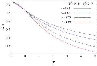
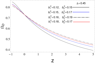
Figure 1: The evolution of $\Omega_{D}$, as a function of $z$, is shown for the present model considering $\Omega_{D0}=0.73$ and different values of $\Delta$, $b_{1}^{2}$ and $b_{2}^{2}$, as mentioned in each panel.

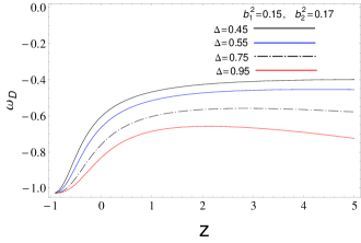
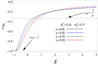
Figure 2: The evolutions of $\omega_{D}$ vs. $z$ (upper panel) and $\omega_{tot}$ vs. $z$ (lower panel), are shown for $\Omega_{D0}=0.73$, $b_{1}^{2}=0.15$, $b_{2}^{2}=0.17$ and different values of $\Delta$, as mentioned in each panel.

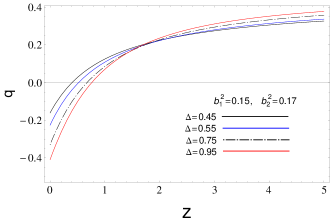
Figure 3: The evolution of $q$, as a function of $z$, is shown for our model considering $\Omega_{D0}=0.73$, $b_{1}^{2}=0.15$, $b_{2}^{2}=0.17$ and different values of $\Delta$, as mentioned in each panel.

III.1 Exact and analytic solutions

Consider now the second Friedmann’s equation which can be written in the equivalent form

$$\left(\left(2-\Delta\right)\Omega_{D0}-2H^{\Delta}\right)\dot{H}$$ (17)

$$+3\left(1-b_{1}^{2}+b_{2}^{2}\right)\Omega_{D0}H^{2}-3\left(1-b_{1}^{2}\right)H^{2+\Delta} = 0$$

where $\Omega_{D0}=(8\pi G/3)C$. The latter equation when $\Delta=\frac{2b_{2}}{b_{1}^{2}-1}$ admits the special exact solution $H\left(t\right)=\frac{2}{3\left(1-b_{1}^{2}\right)\left(t-t_{0}\right)}$. The latter exact solution describes the epoch when the universe is dominated by an ideal gas with equation of state parameter $\omega_{tot}=-b_{1}^{2}$, that is, it describes the solution at point $P_{1}$.

Thus for arbitrary parameter $\Delta$, we observe that  that the singular behaviour $H\left(t\right)=\frac{2}{3\left(1-b_{1}^{2}\right)\left(t-t_{0}\right)}$ it is not an exact solution but describes the leading terms of the second Friedmann’s equation near the singularity $t-t_{0}=0$. Consequently, the singularity analysis can be applied in order to determine the analytic solution of the field equations. Singularity analysis is a powerful method for the determination of analytic solutions for differential equations, as also for the study of the integrability property for a given system. Nowadays, the singularity analysis it is summarized in the so-called Ablowitz, Ramani and Segur algorithm Abl1 ; Abl2 ; Abl3 , known also as ARS algorithm. The latter method provides necessary information if a given differential equation passes the Painlevé test and consequently if the solution of the differential equation can be written as a Laurent expansion around a movable singularity. This method has been widely applied in gravitational studies, for instance see miritzis ; cots1 ; cots2 ; bun2 ; cots ; sinFR ; sinFR2 ; sinFT ; sinr02 and references therein.

There are three main steps for the ARS algorithm. The first step is the determination of the leading-order behaviour, which we have already found it in our approach. The second step has to do with the position of the resonances. We replace

$$H\left(t\right)=\frac{2}{3\left(1-b_{1}^{2}\right)\left(t-t_{0}\right)}+\varepsilon t^{-1+S},$$ (18)

in equation (III.1) and we linearize around $\varepsilon\rightarrow 0$. From the leading-order terms we end with the algebraic equation for the resonance $S+1=0$, that is $S=-1$, which indicates that the singularity is movable. Because the differential equation is of first order we do not have to continue our analysis, however for completeness on the presentation we proceed with the third-step of the ARS algorithm, the consistency test.

For the consistency test we select $\Delta=\frac{1}{2}$ and we replace $H\rightarrow\mathcal{H}^{2}$. Hence, we end with the analytic solution expressed in the Laurent Series

$$\mathcal{H}\left(t\right)=H_{0}\left(t-t_{0}\right)^{-\frac{1}{2}}+H_{1}+H_{2}\left(t-t_{0}\right)^{\frac{1}{2}}$$ (19)

$$+H_{3}\left(t-t_{0}\right)+...+H_{N}\left(t-t_{0}\right)^{-\frac{1}{2}+\frac{N}{2}}$$

where

$$H_{0}=\sqrt{\frac{2}{3\left(1-b_{1}^{2}\right)}}~{},~{}H_{1}=\frac{\left(b_{1}^{2}-1-4b_{2}^{2}\right)}{12\left(b_{1}^{2}-1\right)}\Omega_{D0}~{},$$

$$H_{2}=-\frac{\left(b_{1}^{2}-1-4b_{2}^{2}\right)\left(5\left(b_{1}^{2}-1\right)-2b_{2}^{2}\right)}{32\sqrt{6}\sqrt{1-b_{1}^{2}}\left(b_{1}^{2}-1\right)}~{},~{}...~{}.$$

We remark that the only integration constant is the location of the singularity $t_{0}$.  Finally, equation (III.1) possess the Painlevé property and it is integrable in terms of the singularity analysis.

IV Thermodynamic Implications of Interacting BHDE

We shall now proceed to study the thermodynamic implications of the interacting BHDE proposed in this paper. To meet our purpose, we wish to consider the dynamical apparent horizon of our homogeneous and isotropic FLRW universe. Then, we shall investigate the GSL by evaluating the first order entropy variation for the physical system bounded by the apparent horizon in the framework of interacting BHDE. This sort of thermodynamic study was initiated by Wang et al. Wang1 and later extended by Saha and Chakraborty Saha1 ; Saha2 ; Chakraborty1 . It must be noted that the GSL in these models were studied by assuming that the apparent horizon is ensowed with the Bekenstein entropy and the Hawking temperature. Very recently, the GSL at the dynamical apparent horizon was studied with the Viaggiu entropy Saha3 ; Mamon1 which have shown some promising results. Although there exist many horizons in Cosmology, but the most relevant one in this context is the dynamical apparent horizon which is a marginally trapped surface with vanishing expansion given by Hayward1 ; Hayward2 ; Bak1

$$R_{A}=\frac{1}{\sqrt{H^{2}+\frac{\kappa}{a^{2}}}},$$ (20)

where $k$ is the spatial curvature which we shall set to zero, consistent with our assumption of a spatially flat universe.

At this juncture, it is worth mentioning that the standard operating procedure for GSL study is to determine the sign of the first order entropy variation of the apparent horizon plus the first order entropy variation of the fluid contained within it. The GSL will be satisfied if this sum is nondecreasing.

The first step in this direction is to employ the first law of thermodynamics (FLT) which will provide us with the first order entropy variation of the fluid. In mathematical terms, the FLT is stated as

$$TdS=dE+pdV,$$ (21)

where, $T$ and $S$ are the temperature and the entropy of the fluid respectively, $V=\frac{4}{3}\pi R_{A}^{3}$ is the volume of the fluid bounded by the horizon, $E=V\rho$ is the internal energy of the fluid, evaluated at the dynamical apparent horizon, and $\rho$ and $p$ are the energy density and the pressure of the fluid respectively.

Thus, the change in entropy of the matter and that of the dark energy become

$$dS_{m} = \frac{1}{T}\left(p_{m}dV+dE_{m}\right),$$ (22)

$$dS_{D} = \frac{1}{T}\left(p_{D}dV+dE_{D}\right).$$ (23)

Note that the temperature $T$ has been kept the same in the above equations due to the establishment of thermal equilibrium amongst different cosmic fluids. Now, dividing equations (22) and (23) by $dt$ both sides, we obtain

$$\dot{S}_{m} = \frac{1}{T}\left(p_{m}4\pi R_{A}^{2}\dot{R}_{A}+\dot{E}_{m}\right),$$ (24)

$$\dot{S}_{D} = \frac{1}{T}\left(p_{D}4\pi R_{A}^{2}\dot{R}_{A}+\dot{E}_{D}\right).$$ (25)

In the above equations, $\dot{R}_{A}=-\dot{H}/{H^{2}}=-\dot{H}R_{A}^{2}$.

Finally, plugging in the time derivatives of

$$E_{D}=\frac{4}{3}\pi R_{A}^{3}\rho_{D},$$ (26)

$$E_{m}=\frac{4}{3}\pi R_{A}^{3}\rho_{m}$$ (27)

into equations (24) and (25) and using equation (7), we arrive at the first order entropy variations of the matter and dark energy, respectively, as Saridakis3

$$\dot{S}_{m} = \frac{1}{T}(1+\omega_{m})\rho_{m}4\pi R_{A}^{2}\left(\dot{R}_{A}-HR_{A}\right),$$ (28)

$$\dot{S}_{D} = \frac{1}{T}(1+\omega_{D})\rho_{D}4\pi R_{A}^{2}\left(\dot{R}_{A}-HR_{A}\right).$$ (29)

Our next task is to determine the first order entropy variation of the dynamical apparent horizon. This horizon is analogous to the event horizon of a black hole and the temperature associated with it is given by Bak1 ; Hawking1 ; Jacobson1 ; Padmanabhan1

$$T_{A}=\frac{1}{2\pi R_{A}}.$$ (30)

As for the entropy, we shall employ the Barrow black hole entropy barrow , with the standard horizon area given by $A_{A}=4\pi R_{A}^{2}$. Thus, we obtain

$$S_{A}=\gamma R_{A}^{\Delta+2},$$ (31)

where $\gamma=(4\pi/A_{0})^{1+\Delta/2}$. At this point, it is customary to assume that in gravitational thermodynamics, the temperature of the dynamical apparent horizon and that of the fluid inside are equal, otherwise a temperature gradient might lead to nonequilibrium thermodynamics Padmanabhan2 ; Izquierdo1 ; Mimoso1 . Moreover, the energy flow might deform the geometry Izquierdo1 . Now, differentiating equation (31), we get

$$\dot{S}_{A}=(\Delta+2)\gamma R_{A}^{\Delta+1}\dot{R}_{A}.$$ (32)

Finally, identifying $T$ in equations (28) and (29) with $T_{A}$ in equation (30), and adding equations (28), (29), and (30), we obtain the total entropy variation of the thermodynamic system bounded by the dynamical apparent horizon Saridakis3 :

$$\dot{S}_{tot} = \dot{S}_{m}+\dot{S}_{D}+\dot{S}_{A}$$ (33)

$$= 8\pi^{2}R_{A}^{3}\left(\dot{R}_{A}-HR_{A}\right)\left[(1+\omega_{d})\rho_{D}+(1+\omega_{m})\rho_{m}\right]$$

$$+ (\Delta+2)\gamma R_{A}^{\Delta+1}\dot{R}_{A}$$

$$= \frac{2\pi}{G}H^{-5}\dot{H}\left\{\dot{H}+H^{2}\left[1-\frac{\gamma G}{2\pi}(\Delta+2)H^{-\Delta}\right]\right\}.$$

In arriving at the last equality, we have used the relations $R_{A}=1/H$ and $\dot{R}_{A}=-\dot{H}R_{A}^{2}$. Now, taking out $H^{2}$ from within the braces on the right hand side of equation (33) and noting that $\dot{H}/{H^{2}}=-1-q$, we obtain

$$\dot{S}_{tot} = \frac{2\pi}{G}H^{-3}\dot{H}\left[-q-\frac{\gamma G}{2\pi}(\Delta+2)H^{-\Delta}\right]$$ (34)

$$= -\frac{2\pi}{G}H^{-3}\dot{H}\left[\frac{(1-3b_{1}^{2})+(3b_{1}^{2}-3b_{2}^{2}-1-\Delta)\Omega_{D}}{2-(2-\Delta)\Omega_{D}}\right]$$

$$- \gamma(\Delta+2)H^{-(3+\Delta)}\dot{H}.$$

Let us now analyze equation (34) mathematically. Observe that, since the parameters $\gamma$ and $\Delta$ are nonnegative, so the second term on the right hand side will be nonnegative if $\dot{H}<0$, i.e., when the cosmic fluids respect the null-energy condition. This latter inequality will also force the expression outside the square brackets in the first term to remain positive. Therefore, in our proposed interacting BHDE model, the GSL will be satisfied if

$$\xi=(1-3b_{1}^{2})+(3b_{1}^{2}-3b_{2}^{2}-1-\Delta)\Omega_{D}\geq 0$$ (35)

due to the fact that the denominator inside the square bracket is always positive. Note that the requirement (35) is sufficient and is by no means necessary for the GSL to be satisfied. Two cases may arise:

1. $1-3b_{1}^{2}\geq 0$: This gives $3b_{1}^{2}\leq 1$ which implies that $3b_{1}^{2}-3b_{2}^{2}-1-\Delta\leq 0$. Thus, in this case, GSL will be satisfied if

   $$\Omega_{D}\leq\frac{|3b_{1}^{2}-1|}{|3b_{1}^{2}-3b_{2}^{2}-1-\Delta|}.$$ (36)

2. $3b_{1}^{2}-1>\mbox{max}\{0,|3b_{2}^{2}-\Delta|\}$: This implies that GSL will be satisfied if

   $$\Omega_{D}>\frac{3b_{1}^{2}-1}{3b_{1}^{2}-3b_{2}^{2}-1-\Delta}.$$ (37)

It must, however, be noted that a third case is mathematically plausible where $0<3b_{1}^{2}-1<|3b_{2}^{2}-\Delta|$, but it turns out that these inequalities lead us to an unphysical scenario: $\Omega_{D}<0$.

If, on the other hand, $\dot{H}>0$, then we might safely deduce that the GSL is violated if the iequality in (35) is satisfied. Again, this is only a sufficient condition for the violation of GSL and is by no means necessary.

Therefore, the above analyses show that the violation of the GSL is a possibility in our proposed interacting BHDE model depending on nature of evolution of the Universe.

V Conclusions

In this work, we have proposed a new interacting HDE model which is based on the recently proposed Barrow entropy barrow , which originates from the modification of the black-hole surface due to some quantum-gravitational effects. As discussed in section II, for $\Delta=0$, the BHDE coincides with the standard HDE, while for $0<\Delta<1$ it leads to a new and interesting cosmological scenario. In particular, we have studied the evolution of a spatially flat FRW universe composed of pressureless dark matter and BHDE that interact with each other through a well-motivated interaction term given by equation (12). By considering the Hubble horizon as the infrared cut-off, we have then studied the behavior of the density parameter of BHDE, the EoS parameter of BHDE and the deceleration parameter, during the cosmic evolution.

It has been found that the BHDE model exhibits a smooth transition from early deceleration era ($q>0$) to the present acceleration ($q<0$) era of the universe. Also, the value of this transition redshift is in well accordance with the current cosmological observations zt1 ; zt2 ; zt3 ; zt4 ; zt5 ; zt6 ; zt7 ; zt8 . As discussed in section II, it has also been found that the evolution behaviors of $\omega_{D}$ and $\omega_{tot}$ are in good agreement with recent observations. The latter behaviour it is justified by the main analysis on the asymptotic behavior for evolution of the field equations, where the de Sitter universe is an attractor for the cosmological model. Furthermore, the analytic solution of the field equations was presented. That result it is essential because we know that the numerical simulations describe actual solutions of the dynamical system.

Finally, we have studied the implications of gravity-thermodynamics in the BHDE model by assuming the dynamical apparent horizon as the cosmological boundary. The apparent horizon is endowed with Hawking temperature and Barrow entropy defined in equations (30) and (31) respectively. In particular, we have examined the viability of the GSL. After a careful mathematical analysis, we have found that there is a possibility of conditional violation of the GSL based on how the Universe undergoes evolution. More precisely, we have obtained certain constraints on the density parameter $\Omega_{D}$ for which the GSL will be satisfied in the case where $\dot{H}<0$, while, on the other hand, we have obtained a condition for the violation of the GSL in the case where $\dot{H}>0$. One must, however, note that these constraints are sufficient in nature and are by no means necessary for the viability of the GSL.

VI Acknowledgments

The authors are thankful to an anonymous reviewer for valuable comments which have helped to improve the presentation of this work.

References

- (1) A. G. Riess et al., Astron. J. 116, 1009 (1998).
- (2) S. Perlmutter et al., Astrophys. J. 517, 565 (1999).
- (3) P.A.R. Ade et al., Astron. Astrophys. 571, A16 (2014).
- (4) D.N. Spergel et al., Astrophys. J. Suppl. Ser. 148, 175 (2003).
- (5) M. Tegmark etal., Phys. Rev. D 69, 103501 (2004).
- (6) E. J. Copeland, M. Sami and S. Tsujikawa, Int. J. Mod. Phys. D. 15, 1753 (2006).
- (7) L. Amendola and S. Tsujikawa, Dark Energy: Theory and Observations, Cambridge University Press, Cambridge, UK (2010).
- (8) K. Bamba, S. Capozziello, S. Nojiri and S. D. Odintsov, Astrophys. Space Sci. 342, 155 (2012).
- (9) G.’t Hooft, Salamfest 1993: 0284-296 [arXiv: gr-qc/9310026].
- (10) L. Susskind, J. Math. Phys. 36, 6377 (1995).
- (11) W. Fischler and L. Susskind, arXiv: hep-th/9806039.
- (12) A. Cohen, D. Kaplan, A. Nelson, Phys. Rev. Lett. 82, 4971 (1999).
- (13) P. Horava and D. Minic, Phys. Rev. Lett. 85, 1610 (2000).
- (14) R. Bousso, Rev. Mod. Phys. 74, 825 (2002).
- (15) M. Li, Phys. Lett. B 603, 1 (2004).
- (16) R. Horvat, Phys. Rev. D 70, 087301 (2004).
- (17) Q. G. Huang and M. Li, JCAP 0408, 013 (2004).
- (18) B. Wang, Y. g. Gong and E. Abdalla, Phys. Lett. B 624, 141 (2005).
- (19) D. Pavon and W. Zimdahl, Phys. Lett. B 628, 206 (2005).
- (20) H. Kim, H. W. Lee and Y. S. Myung, Phys. Lett. B 632, 605 (2006).
- (21) S. Nojiri and S. D. Odintsov, Gen. Rel. Grav. 38, 1285 (2006).
- (22) M. R. Setare, Phys. Lett. B 642, 1 (2006).
- (23) B. Wang, C. Y. Lin and E. Abdalla, Phys. Lett. B 637, 357 (2006).
- (24) M. R. Setare and E. N. Saridakis, Phys. Lett. B 670, 1 (2008).
- (25) S. Wang, Y. Wang and M. Li, Phys. Rept. 696, 1 (2017).
- (26) E. N. Saridakis, K. Bamba, R. Myrzakulov and F. K. Anagnostopoulos, JCAP 12, 012 (2018).
- (27) S. Nojiri, S. D. Odintsov and E. N. Saridakis, Phys. Lett. B 797, 134829 (2019).
- (28) R. G. Cai, Phys. Lett. B 657, 228 (2007).
- (29) C. Q. Geng, Y. T. Hsu, J. R. Lu and L. Yin, Eur. Phys. J. C 80, 21 (2020).
- (30) E. N. Saridakis, Phys. Lett. B 660, 138 (2008).
- (31) M. R. Setare and E. C. Vagenas, Int. J. Mod. Phys. D 18, 147 (2009).
- (32) Y. Gong and T. Li, Phys. Lett. B 683, 241 (2010)
- (33) Y. G. Gong, Phys. Rev. D 70, 064029 (2004).
- (34) L. N. Granda, A. Oliveros, Phys. Lett. B 669, 275 (2008).
- (35) X. Zhang and F. Q. Wu, Phys. Rev. D 72, 043524 (2005).
- (36) C. Feng, B. Wang, Y. Gong and R. K. Su, JCAP 0709, 005 (2007).
- (37) M. Li, X. D. Li, S. Wang and X. Zhang, JCAP 0906, 036 (2009).
- (38) X. Zhang, Phys. Rev. D 79, 103509 (2009).
- (39) J. Lu, E. N. Saridakis, M. R. Setare and L. Xu, JCAP 1003, 031 (2010).
- (40) A. A. Mamon, Int. J. Mod. Phys. D 26, 1750136 (2017).
- (41) E. Sadri, Eur. Phys. J. C 79, 762 (2019).
- (42) R. D’Agostino, Phys. Rev. D 99, 103524 (2019).
- (43) J. D. Barrow, Phys. Lett. B 808, 135643 (2020).
- (44) J. D. Bekenstein, Lett. Nuovo Cim. 4, 737 (1972).
- (45) J. D. Bekenstein, Phys. Rev. D 7, 2333 (1973).
- (46) E. N. Saridakis, Phys. Rev. D 102, 123525 (2020).
- (47) F. K. Anagnostopoulos, S. Basilakos, E. N. Saridakis, Eur. Phys. J. C 80, 826 (2020).
- (48) Y. L. Bolotin, A. Kostenko, O. A. Lemets and D. A. Yerokhin, IJMPD, 24, 1530007 (2015).
- (49) E. Di Valentino, A. Melchiorri and O. Mena, Phys. Rev. D 96, 043503 (2017).
- (50) S. Kumar and R. C. Nunes, Phys. Rev. D 96, 103511 (2017)
- (51) C. Tsallis, J. Statist. Phys. 52, 479 (1988).
- (52) C. Tsallis and L. J. L. Cirto, Eur. Phys. J. C 73, 2487 (2013).
- (53) S. D. H. Hsu, Phys. Lett. B 594, 13 (2004).
- (54) A. Sheykhi, Class. Quantum Grav. 27, 025007 (2010).
- (55) M. Quartin et al., J. Cosmol. Astropart. Phys, 05, 007 (2008).
- (56) D. Pavon and B. Wang, Gen. Rel. Grav. 41, 1 (2009).
- (57) C. G. Boehmer, G. Caldera-Cabral, R. Lazkoz, and R. Maartens, Phys. Rev. D 78, 023505 (2008).
- (58) G. Caldera-Cabral, R. Maartens, and L. A. Urena-Lopez, Phys. Rev. D 79, 063518 (2009).
- (59) A. A. Mamon, A. H. Ziaie and K. Bamba, Eur. Phys. J. C 80, 974 (2020).
- (60) L. P. Chimento, Phys. Rev. D 81, 043525 (2010).
- (61) G. Papagiannopoulos, P. Tsiapi, S. Basilakos and A. Paliathanasis, EPJC 80, 55 (2020).
- (62) S. Pan, W. Yang and A. Paliathanasis, MNRAS 493, 3114 (2020).
- (63) W. Yang, S. Pan, E. Di Valentino, R.C. Nunes, S. Vagnozzi and D.F. Mota, JCAP 09, 019 (2018).
- (64) W. Yang, A. Mukherjee, E. Di Valentino and S. Pan, Phys. Rev. D 98, 123527 (2018).
- (65) W. Yang, S. Pan and A. Paliathanasis, MNRAS 482, 1007 (2019).
- (66) T. Gonzalez, G. Leon and I. Quiros, Class. Quantum Grav. 30, 135001 (2013).
- (67) G. Leon, Class. Quantum Grav. 26, 035008 (2009).
- (68) A. Giacomini, G. Leon, A. Paliathanasis and S. Pan, Eur. Phys. J. C 80, 1 (2020).
- (69) R. Lazkoz, G. Leon and I. Quiros, Phys. Lett. B 649, 103 (2007).
- (70) O. Farooq, B. Ratra, Astrophys. J. 766, L7 (2013).
- (71) O. Farooq, F. R. Madiyar, S. Crandall, B. Ratra, ApJ 835, 26 (2017).
- (72) A. A. Mamon, K. Bamba, S. Das, Eur. Phys. J. C 77, 29 (2017).
- (73) A. A. Mamon and K. Bamba, Eur. Phys. J. C 78, 862 (2018).
- (74) J. Magana et al., J. Cosmol. Astropart. Phys. 10, 017 (2014).
- (75) A. A. Mamon, S. Das, Int. J. Mod. Phys. D. 25, 1650032 (2016).
- (76) A. A. Mamon, S. Das, Eur. Phys. J. C 77, 495 (2017).
- (77) A. A. Mamon, Mod. Phys. Lett. A 33, 1850056 (2018).
- (78) M.J. Ablowitz, A. Ramani and H. Segur, Lettere al Nuovo Cimento 23 333 (1978).
- (79) M.J. Ablowitz, A. Ramani and H. Segur, J. Math. Phys. 21 715 (1980).
- (80) M.J. Ablowitz, A. Ramani and H. Segur, J. Math. Phys. 21 1006 (1980).
- (81) J. Miritzis, P.G.L. Leach and S. Cotsakis, Grav. Cosmol. 6 282 (2000).
- (82) S. Cotsakis and P.G.L. Leach, J. Phys A 27, 1625 (1994).
- (83) P.G.L. Leach, S. Cotsakis and J. Miritzis, Grav. Cosmol. 7, 311 (2000).
- (84) T. Bountis and L. Drossos, On The Non-Integrability of the Mixmaster Universe Model. In: Simó C. (eds) Hamiltonian Systems with Three or More Degrees of Freedom. NATO ASI Series (Series C:Mathematical and Physical Sciences), vol 533. Springer, Dordrecht (1999).
- (85) S. Cotsakis, J. Demaret, Y. De Rop and L. Querella, Phys. Rev. D 48, 4595 (1993).
- (86) A. Paliathanasis and P.G.L. Leach, Phys. Lett. A 380, 2815 (2016).
- (87) A. Paliathanasis, EPJC 77, 438 (2017).
- (88) A. Paliathanasis, J.D. Barrow and P.G.L. Leach, Phys. Rev. D 94, 023525 (2016).
- (89) S. Cotsakis, S. Kadry, G. Kolionis and A. Tsokaros, Phys. lett. B 755, 387 (2016).
- (90) B. Wang, Y. Gong, and E. Abdalla, Phys. Rev. D 74, 083520 (2006).
- (91) S. Saha and S. Chakraborty, Phys. Lett. B 717, 319 (2012).
- (92) S. Saha and S. Chakraborty, Phys. Rev. D 89, 043512 (2014).
- (93) S. Chakraborty and S. Saha, Mod. Phys. Lett. A 30, 1550024 (2015).
- (94) S. Saha, Int. J. Mod. Phys. A 34, 1950193 (2019).
- (95) A. A. Mamon and S. Saha, Int. J. Mod. Phys. D, 29, 2050097 (2020).
- (96) S. A. Hayward, Class. Quant. Grav. 15, 3147 (1998).
- (97) S. A. Hayward, S. Mukohyama and M. Ashworth, Phys. Lett. A 256, 347 (1999).
- (98) D. Bak and S. J. Rey, Class. Quant. Grav. 17, L83 (2000).
- (99) E. N. Saridakis and S. Basilakos, arXiv: 2005.08258 (2020).
- (100) S. W. Hawking, Commun. Math. Phys. 43, 199 (1975).
- (101) T. Jacobson, Phys. Rev. Lett. 75, 1260 (1995).
- (102) T. Padmanabhan, Class. Quant. Grav. 19, 5387 (2002).
- (103) T. Padmanabhan, Rept. Prog. Phys. 73, 046901 (2010).
- (104) G. Izquierdo and D. Pavón, Phys. Lett. B 633, 420 (2006).
- (105) J P. Mimoso and D. Pavón, Phys. Rev. D 94, 103507 (2016).