The regularized Stokeslets method applied to the three-sphere swimmer model.

Abstract

We investigate the applicability of the Method of Regularized Stokeslets (MRS) in the simulation of micro-swimmers at low Reynolds number. The chosen model for the study is the well-known three linked spheres swimmer. We compare our results with the lattice Boltzmann method, multiparticle collision dynamics, a numerical solution of the Oseen tensor equation and an analytical solution, all taken from Earl et al. [J. Chem. Phys. 126, 064703 (2007)]. The MRS is studied in detail, and our results show an excellent agreement with the lattice Boltzmann method, and with the analytical solution in its range of validity. We conclude that the MRS is well suited for this type of simulation, offering advantages such as being easy to implement and to represent complex geometries. Therefore it presents itself as a suitable candidate for more complex simulations.

I Introduction

The interest in the study and development of microswimmers has been growing in the past years.
Microswimmers are mechanisms, whether biological or not, of microscopic dimensions that propels itself in a fluid. Some examples are biological creatures like bacteria and human-made micro-robots. The study of the individual and collective behaviour of these small machines has led to the discovery of many new and curious phenomena, and they are currently objects of interest in many lines of research Gompper et al. (2020).

The locomotion and interaction of microscopic swimmers in newtonian and incompressible fluids can be studied using the mechanical equations. At such small scales and low velocities, the Reynolds number is small, and a simplified linear approximation of the Navier-Stokes equations can be used Childress (2009). The linear Stokes equations, as it is called, is obtained by disregarding the inertial terms, given the dominance of the viscous force at this scale. In this process, we remove any non-linear term, and also any time dependence from the equations.

The inexistence of time reflects the fact that at this regime, fluids respond instantly to perturbations, and they dictate the time evolution of the physical quantities of the fluid. As a consequence, if a force suddenly stops acting on the fluid, the generated flow also vanishes suddenly. Additionally, any time external forces are inverted, an inverted flow pattern takes place. These and other properties make low Reynolds number flows unique, and are responsible for some very curious phenomena, such as the possibility to reverse fluid mixing under certain circumstances Fonda and Sreenivasan (2017). They also impose a set of conditions for autonomous swimming.

As explained by Purcell in his famous paper Purcell (1977), only mechanisms that execute a nonreciprocal sequence of movements, that is, movements that do not look the same when analyzed backwards in time, are capable of travelling arbitrary long distances in such environments. One of the simplest swimmers that satisfies these conditions is the three-sphere swimmer proposed in 2004 by Najafi and Golestanian Najafi and Golestanian (2004) and further analyzed in 2008 Golestanian and Ajdari (2008). Since then, this model has been extensively studied by numerical, analytical and experimental methods Nasouri, Vilfan, and Golestanian (2019); Leoni et al. (2009); Farzin, Ronasi, and Najafi (2012). Because of its simplicity and the possibility of analytical studies, it can serve as a good initial test for numerical methods that may later be used for more complex systems (although there is another simple model Avron, Kenneth, and Oaknin (2005) that could also be used).

The study of such mechanisms by means of the linear equations is not always trivial. The linearization is generally not enough to make the task of predicting fluid behaviour easy. Usually, only trivial cases with simple geometries or few constituents can be studied analytically in great detail. For this reason, there is still interest in the development and study of new methods for simulating low Reynolds number interactions. Nowadays, highly used methods for these situations are the multi-particle collision dynamics (MPC) and the lattice Boltzmann method (LBM). Both have very different approaches, merits and limitations. The MPC and LBM methods, together with a numerical solution of the Oseen tensor equations (OTE) and an analytical approximation, have been explained and compared in the specific case of the three linked spheres swimmer in Earl et al. (2007). Here, based on this work, we proceeded to add a fourth method in the comparison, namely the Method of Regularized Stokeslets (MRS) Cortez (2001). For this comparison, we implemented the MRS for the same system to compare to MPC, LBM, OTE and the analytical approximation. Our results show that the MRS is well suited for this type of simulation, showing good agreement with the analytical solution in the valid domain. We finish by concluding that the MRS is a useful tool to be used in the study of interactions at low Reynolds number. We also discuss the peculiarities of the method and its numerical implementation details.

II The method of regularized Stokeslets

The MRS is based on a slight modification of the Green function method for the linear Stokes equations. The Green function response for a delta distribution has a singularity at the perturbation point. Therefore it is not much useful when used in discrete combinations, since it adds singularities to the flow, not being very representative of any physical behaviour. It can be useful in situations where the force of interaction on a continuous boundary is known at each point, or a realistic one can be guessed. In this case, it can be integrated to give the total flow generated by this interaction.

In contrast with the standard Green method, in the MRS, the delta distribution is replaced by a smooth, radially symmetric and normalized function over the whole space. This function is controlled by a parameter $\epsilon>0$ that determines how localized the force is.
The equations to be solved are:

$$\mu\nabla^{2}\bm{u}=\nabla p-\bm{f}\phi_{\epsilon}$$ (1)

$$\nabla\cdot\bm{u}=0$$ (2)

Where $\bm{u}$ is the fluid velocity, $\mu$ is the viscosity, $p$ is the pressure, $\bm{f}$ is a constant vector representing the interaction force and

$$\phi_{\epsilon}=f(\bm{x})=g(\left|\bm{x}-\bm{x_{0}}\right|)$$ (3)

is the chosen regularized delta, dependent only on the distance from the perturbation $\bm{x}_{0}$.
In this paper, we use the amply used $\phi_{\epsilon}(r)$ given by Cortez (2001) and shown in Fig. 1.

$$\phi_{\epsilon}(r)=\frac{15\epsilon^{4}}{8\pi(r^{2}+\epsilon^{2})^{7/2}}$$ (4)

Figure 1: $\phi_{\epsilon}$ given in Eq. (3) for the indicated parameters, a smaller $\epsilon$ results in a taller and more localized function. It approximates a Dirac delta in the limit $\epsilon\rightarrow 0$.

Equations (1) and (2) are solved by:

$$\mu\bm{u}(\bm{x})=(\bm{f}\cdot\nabla)\nabla B_{\epsilon}(\bm{x}-\bm{x}_{0})-\bm{f}G_{\epsilon}(\bm{x}-\bm{x_{0}})$$ (5)

valid for the 2D and 3D cases (derived in Cortez (2001) together with an expression for the pressure). $G_{\epsilon}(r)$ and $B_{\epsilon}(r)$ are auxiliary functions defined as solutions of $\nabla^{2}G_{\epsilon}(r)=\phi_{\epsilon}(r)$ and $\nabla^{2}B_{\epsilon}(r)=G_{\epsilon}(r)$, for $r=\left|\bm{x}-\bm{x}_{0}\right|$ and, in all equations the vector operators act on the cartesian coordinates $\bm{x}$.

Interestingly, this type of perturbation generates a finite and non-singular response at the point of perturbation, allowing the no-slip condition to be imposed at $\bm{x}=\bm{x}_{0}$, leading to the possibility of using these perturbations to represent small particles. The response now can be interpreted as a velocity field generated by a mean interaction over a ball. We can also use a finite, discrete and closely placed set of such perturbations to represent a surface interaction. Since the equations (1) and (2) are linear, the velocity response of multiple perturbations can be constructed by a linear combination. If we have $N$ interactions with the fluid, each one exerting a force $\bm{f}_{k}$ at points $\bm{x}_{k}$, we can build the solution:

$$\bm{u}(\bm{x})=\bm{U}_{0}+\frac{1}{\mu}\sum^{N}_{k=1}{(\bm{f}_{k}\cdot\nabla)\nabla B_{\epsilon}(r_{k})-\bm{f}_{k}G_{\epsilon}(r_{k})}$$ (6)

for $r_{k}=\left|\bm{x}-\bm{x_{k}}\right|$. The expression within the summation can be expanded and simplified given that $B$ and $G$ are dependent on $\left|\bm{x}-\bm{x_{k}}\right|$ only, as also shown in Cortez (2001). Given a choice of $\phi_{\epsilon}$ we can find both $G$ and $B$ by supposing $G$ and $B$ radially symmetric. Any constant of integration can be adjusted so that there is no flow for $r\rightarrow\infty$ (this is possible in three dimensions), and to make the velocity finite at each perturbation ($r=0$). Any other constant term can be eliminated by the choice of $\bm{U}_{0}$, in our case we can set $\bm{U}_{0}=\bm{0}$.

Eq. (6) can be used to compute flows if we know the forces of interaction. In general, we only know the velocities of each point, and due to the regularization, the no-slip condition can be imposed at each point $\bm{x}_{i}$:

$$\bm{u}(\bm{x}_{i})=\frac{1}{\mu}\sum^{N}_{k=1}{(\bm{f}_{k}\cdot\nabla)\nabla B_{\epsilon}(r_{ik})-\bm{f}_{k}G_{\epsilon}(r_{ik})}$$ (7)

where $r_{ik}=\left|\bm{x}_{i}-\bm{x}_{k}\right|$. This sum can be seen as:

$$\bm{u}(\bm{x}_{i})\equiv\bm{u}_{i}=\sum^{N}_{k=1}\bm{M(r_{ik})}\bm{f}_{k}$$ (8)

where each term is composed of a linear operator $\bm{M}$ dependent on the distances, acting on $\bm{f}_{k}$. If $D$ is the dimension, the operator $\bm{M}$ acts on $\mathbb{R}^{D}$, and its matrix representation has size $D^{2}$. However, the whole system can be seen as a linear system in $\mathbb{R}^{DN}$:

$$\mathcal{U=MF}$$ (9)

if we treat $\mathcal{U}$ and $\mathcal{F}$ as augmented vectors of size $D\cdot N$ and $\mathcal{M}$ as the augmented matrix of all $\bm{M}$’s. Since now we know the velocity of each particle, we can solve Eq. (9) numerically for the forces and then return to Eq. (6) to compute the flow. Generally, the matrix $\mathcal{M}$ is not invertible, but we can find solutions with iterative methods. In this paper, we used GMRES with zero initial guess in every case. With a choice of $\phi_{\epsilon}$ we can find the auxiliary functions, and then the expressions for each operator $\bm{M}$ and consequently for $\mathcal{M}$. Recalling $\phi_{\epsilon}$ from Eq. (3), the expression for the operator is:

$$\left[\bm{M}(r_{ik})\right]_{lm}=\frac{1}{\mu}\{F_{1}(r_{ik})\delta_{lm}+F_{2}(r_{ik})(\bm{r}_{ik})_{l}(\bm{r}_{ik})_{m}\}$$ (10)

with:

$$F_{1}(r)=\frac{1}{8\pi}\frac{r^{2}+2\epsilon^{2}}{(r^{2}+\epsilon^{2})^{3/2}}\\$$ (11)

$$F_{2}(r)=\frac{1}{8\pi(r^{2}+\epsilon^{2})^{3/2}}$$ (12)

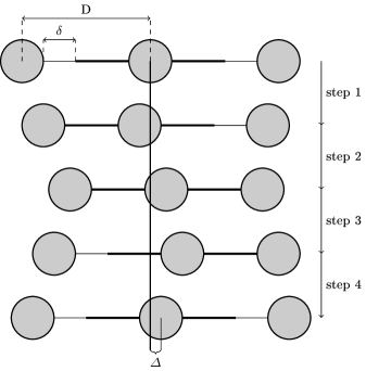
Figure 2: Qualitative view of the swimmer motion in a complete cycle. After four steps it returns to its original configuration, but in a different location.

III The three-sphere swimmer

For the comparison, we analysed the swimmer proposed in Najafi and Golestanian (2004) and studied by multiple methods in Earl et al. (2007), the three-sphere swimmer. This swimmer consists of three spheres of radius $R$, connected on a line by two arms of negligible thickness. The swimmer moves by changing its arm’s lengths in a specific manner so that the complete sequence is non-reciprocal. The complete cycle consists of four steps, wherein at each step, one arm is kept fixed while the length of the other is changed by an amount we define as $\delta$ with a constant rate. That is illustrated in Fig. 2. After one complete cycle, the swimmer returns to its original configuration, and we measure $\Delta$, the translated distance.

IV Numerical Study

IV.1 Validation and tests

Before using the method for the swimmer, we decided to validate and test our implementation with the case of a single sphere translating with constant velocity, a case for which we had data to compare Cortez, Fauci, and Medovikov (2005); Thompson (2015). Also, since the swimmer consists of three translating spheres, we used these tests to decide what values of $N$, $\epsilon$ and what type of discretization to use.

The choice of $N$ must be carefully taken since it is the parameter that has the biggest impact on computational time and memory usage. We recall that the matrix $\mathcal{M}$ has $(ND)^{2}$ terms. Ideally, for the best precision, $N$ should be set as big as possible, with $\epsilon$ approaching zero. If $N$ is too small, the set of points will not represent well the surface of the sphere, and we would get poor results. Due to the limited memory and computing power, we must find a balance between memory, speed and precision. A drawback of the method is that the matrix $\mathcal{M}$, Eq. (9), is generally not sparse. Its sparsity depends on the configuration of the points. Because of that, it is not possible to reduce memory usage by using alternative storage methods for sparse matrices. Luckily the MRS enables us to get good results by using the strategy of decreasing the number of points and increasing the volume of interaction by increasing $\epsilon$, and in general, as in the case of our simulations, memory requirements were easily achievable.

For every value of $N$, we have to adjust $\epsilon$. There is no general rule to find the best value of $\epsilon$ for a given $N$ Garcia-Gonzalez (2016). In general, it depends upon the distances between points. Our approach is to choose $\epsilon$ after defining $N$, by varying it until we get enough precision. For this set-up, the total force was a well behaved function of $\epsilon$, and for every $N$, there was a single point of minimization of the error, similar to Fig. 4 in Thompson (2015), so we set $\epsilon$ as close to this point as desired. For the discretization method, since we are using the same $\epsilon$ for every point, we looked for placing the points as equally spaced as possible. However, there is no perfect way to place $N$ equally spaced points on a sphere. Three techniques and their implications while using this method were discussed in Thompson (2015). Besides that, the symmetry of the discretization must be taken into consideration.

We first tested a Fibonacci lattice since it is a very simple rule and generates very uniform distributions. The sphere was translated in the $x$-direction. We used $N=1800$, which showed to be more than enough for our purposes, and $R=3$ since this is the radius of the spheres of the swimmer. We compared the modulus of the total force and torque obtained numerically, which in this case are respectively:

$$\bm{F}=\sum^{N}_{k=1}\bm{-f}_{k}\\$$ (13)

$$\bm{T}=\sum^{N}_{k=1}\bm{r}_{k}\times-\bm{f}_{k}$$ (14)

(given the origin set in the central point of the sphere), with the known analytical expressions for the sphere: $F=6\pi\mu a|u|$ and $T=8\pi\mu a^{3}|\Omega|$. For this $N$, we did achieve enough precision for the force for the value of $\epsilon$ that is shown in Table 1. We were getting very proximate values for the total force, however the $y$ and $z$ components were different from zero by a tiny amount, and we were measuring a very small, but not zero net torque, for both sideways and upward translations. This is was also reported in Thompson (2015), and it is not in agreement with the analytical predictions of zero torque for pure translations. This is expected because the discretization is not perfectly symmetric, as shown in Fig. 3.

(a)

(b)

Figure 3: Side (left) and up view (right) of the discretized sphere with 1800 points and $R=3$, using a Fibonacci lattice.

However, later we verified that this torque was small enough to be ignored, and for this case, we could have just ignored any rotation or movement out of the $x$ axis.

But because of these small discrepancies, we decided to test another method of discretization, known as cubed-sphere or box to sphere. In this discretization, we place the points by projecting a uniform square grid on the surface of the sphere, as illustrated in Fig. 4.

Figure 4: Cubed-sphere discretization for a $16\times 16$ grid in each face, with $R=3$. This face was translated in the $x$ direction.

Although this discretization is not as uniform as the previous one, it has multiple planes of symmetry. We obtained very precise values for the total force and, we reproduced exactly the values obtained in Cortez, Fauci, and Medovikov (2005). We have now obtained zero torque in every case since $xy$ and $zx$ are planes of symmetry. As it was stated in Thompson (2015), as long as we use a large number of points, the non uniformity of the discretization is not so important for precision on the total force. However, we must add that the symmetry may be an important factor, as this case suggests. For this discretization method, we used grids with $16\times 16$ points, that means a total of $N=6\times 16^{2}=1536$ points. The value of $\epsilon$ is shown on Table 1.

Table 1: Values of $N$ and $\epsilon$ used for each discretization type in the simulation of the swimmer.

	Fibonacci lattice	Cubed-sphere
$N$	1800	1536
$\epsilon$	0.0942797519	0.1095680485

IV.2 Simulation of the three-sphere swimmer

The swimmer is modelled by three spheres, discretized by the methods discussed in section IV.1. For each discretization type, we used the number of points and the values of $\epsilon$ of Table 1.
The method implementation for the swimmer requires some adaptations since now we are dealing with moving boundaries. Mainly, we need to recompute matrix $\mathcal{M}$ at each step, and to determine the velocities of each sphere. Since we are interested in studying autonomous swimming, we must find solutions that satisfy at every step, the following conditions:

$$\sum^{N}_{k=1}\bm{f}_{k}=0$$ (15)

and:

$$\sum^{N}_{k=1}\bm{r}_{k}\times\bm{f}_{k}=0$$ (16)

which means that the movement does not require any external forces or torques. Condition Eq. (16) can be satisfied by taking the same precautions as the case of a single sphere. Again, only by analyzing the swimmer and its symmetry, we can conclude that no torque should act on it during any of its steps. So if we use a proper symmetric discretization, this condition is automatically satisfied in any longitudinal motion of the spheres. However, as in the case of the Fibonacci lattice, the asymmetry is so small that the resulting small torque is negligible.

To satisfy Eq. (15) we needed a more subtle mechanism.

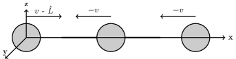
Figure 5: Example of the first step of the swimmer and the respective velocities.

We will exemplify how we proceed using the first step as an example, but this argument is valid for all swimming steps. By the construction of the swimmer, at every step, we have the constraint that one arm is retracting or extending with a given constant rate, which we call $\dot{L}$, while the other remains fixed. To satisfy this constraint, we can set the velocity of each sphere, as illustrated in Fig. 5, with $\dot{L}$ negative, if the arm is retracting; $v$ is an arbitrary velocity, and all the vectors are in the direction $\bm{\hat{\imath}}$. With this setup, for any value of $v$, which is measured relative to the fluid, we have the execution of step one, but to satisfy Eq. (15) we have to find the specific value of $v$ that will result in a total null force. Because of the symmetry, we expect for any motion of this type, that the $y$ and $z$ force components sum up to zero. If that is the case, the total force will be given simply by $\bm{F}=F_{x}\bm{\hat{\imath}}$, and now, because of the linear relation Eq. (9), it will depend linearly on $v$.

$$F_{x}=mv+b$$ (17)

Using that, we find the correct value of $v$ by solving two linear systems for the forces with two arbitrary values of $v$, computing the respective total forces and with these two values finding the root of Eq. (17). With this $v$ we update the positions with:

$$\bm{r}_{k}(t+\delta t)=\bm{r}_{k}(t)+\bm{u}_{k}(t)\delta t$$ (18)

This process is repeated, verifying if it is time to go to the next step of the swimming motion until the cycle is complete. When one complete cycle is executed, we measure the displacement $\Delta$.

V Results

Since our aim is to compare the MRS with other methods that were implemented in Earl et al. (2007), we used the same parameters of this work: $R=3$ and $D=25$. The simulation is done by varying the parameter $\delta$ and computing the net displacement $\Delta$ after one complete cycle. We present our data in Fig. 6 by plotting our results directly on top of the data from Earl et al. (2007) (with permission) . Our result is shown with a dotted line. The data is presented by the relation between the dimensionless variables $\Delta/R$ and $\delta/D$. What we call $\delta$ was denoted by $\bm{\varepsilon}$ in the original figure. We ran two simulations for the swimmer. In each one, we discretized the spheres by each method discussed previously and used the same number of points and $\epsilon$ from Table 1. However, the results are visually indistinguishable, so we are showing only one of the curves.

This figure shows that the results with the MRS are in very good agreement with the analytical solution (dashed line) for $\delta<<D$ and $R<<D$. For higher values of $\delta/D$, when the analytical solutions are no longer valid, our solutions are very close to the LBM (crosses mark) and MPC (error bars), both methods that are supposed to work in this range. This indicates a good behaviour of the MRS for the range of all values of $\delta/D$. We note that the dot-dashed line, which is an analytical solution from Najafi and Golestanian (2004), is good for high $\delta/D$ but does not converge for small values, an assumption initially made in its deduction. That formula was corrected in Earl et al. (2007) and is shown in Fig. 6 by the dashed line.

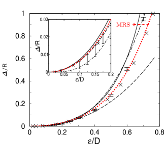
Figure 6: Figure taken from Earl et al. (2007) with our result plotted on top with doted line. In this figure, $\bm{\varepsilon}$ is what we denoted as $\delta$. The solid line is obtained by solving the Oseen tensor equations numerically, the crosses mark is obtained with the lattice Boltzmann, the error bars show the results obtained by multiparticle collision dynamics, which is a noisy method, the dashed and dotted dashed lines are theoretical solutions for $\delta<<R$ and $R<<D$ obtained respectively by Najafi and GolestanianNajafi and Golestanian (2004) and by the authors of Earl et al. (2007).

VI Conclusion

Although the MRS is already being used in a great variety of applications, we felt that simpler and more careful tests were lacking in the literature, specifically addressing micro-swimmers, in order to explore the details and capabilities of this method. Here, we filled this gap by using the MRS to study one of the simplest models of micro-swimmers, the three-sphere swimmer. This swimmer was already studied by other numerical and analytical methods, providing us with material to compare.

First, we have discussed and explained the theory behind the MRS, showing how it is a different approach to the Stokes equations, and how the regularization of the perturbation changes the interpretation of the response, increasing the possibilities of use.

We implemented and tested the method for the case of a single translating sphere, showing the importance of each parameter and discretization type, and how we achieved a balance between precision, memory usage and speed. We showed two examples of discretizations and what effects each one had in the final results, achieving good precision for the total force in both cases.

We then studied the autonomous swim of the three-sphere swimmer numerically. We modelled the swimmer by using three discretized spheres. We tested both discretization methods, obtaining similar results for each one. By comparing our results with results from other methods and with an analytical solution taken from Earl et al. (2007), we showed that the MRS performed very well, agreeing nicely with the analytical solution in its range of validity, and staying closer to the LBM results in higher ranges. This is a good indication of the reliability of the method.

We conclude that the MRS is a simple, useful and precise tool to be used in the study of interactions at low Reynolds number.

data AVAILABILITY

The data that support the findings of this study are available from the corresponding author upon reasonable request.

References

- Gompper et al. (2020) G. Gompper, R. G. Winkler, T. Speck, A. Solon, C. Nardini, F. Peruani, H. Löwen, R. Golestanian, U. B. Kaupp, L. Alvarez, T. Kiørboe, E. Lauga, W. C. K. Poon, A. DeSimone, S. Muiños-Landin, A. Fischer, N. A. Söker, F. Cichos, R. Kapral, P. Gaspard, M. Ripoll, F. Sagues, A. Doostmohammadi, J. M. Yeomans, I. S. Aranson, C. Bechinger, H. Stark, C. K. Hemelrijk, F. J. Nedelec, T. Sarkar, T. Aryaksama, M. Lacroix, G. Duclos, V. Yashunsky, P. Silberzan, M. Arroyo, and S. Kale, “The 2020 motile active matter roadmap,” Journal of Physics: Condensed Matter 32, 193001 (2020).
- Childress (2009) S. Childress, An Introduction to Theoretical Fluid Mechanics (AMS and Courant Institute of Mathematical Sciences at New York University, 2009).
- Fonda and Sreenivasan (2017) E. Fonda and K. R. Sreenivasan, “Unmixing demonstration with a twist: A photochromic Taylor-Couette device,” American Journal of Physics 85, 796–800 (2017), https://doi.org/10.1119/1.4996901 .
- Purcell (1977) E. M. Purcell, “Life at low Reynolds number,” American Journal of Physics 45, 3–11 (1977), https://doi.org/10.1119/1.10903 .
- Najafi and Golestanian (2004) A. Najafi and R. Golestanian, “Simple swimmer at low Reynolds number: Three linked spheres,” Phys. Rev. E 69, 062901 (2004).
- Golestanian and Ajdari (2008) R. Golestanian and A. Ajdari, “Analytic results for the three-sphere swimmer at low Reynolds number,” Phys. Rev. E 77, 036308 (2008).
- Nasouri, Vilfan, and Golestanian (2019) B. Nasouri, A. Vilfan, and R. Golestanian, “Efficiency limits of the three-sphere swimmer,” Phys. Rev. Fluids 4, 073101 (2019).
- Leoni et al. (2009) M. Leoni, J. Kotar, B. Bassetti, P. Cicuta, and M. C. Lagomarsino, “A basic swimmer at low reynolds number,” Soft Matter 5, 472–476 (2009).
- Farzin, Ronasi, and Najafi (2012) M. Farzin, K. Ronasi, and A. Najafi, “General aspects of hydrodynamic interactions between three-sphere low-reynolds-number swimmers,” Phys. Rev. E 85, 061914 (2012).
- Avron, Kenneth, and Oaknin (2005) J. E. Avron, O. Kenneth, and D. H. Oaknin, “Pushmepullyou: an efficient micro-swimmer,” New Journal of Physics 7, 234–234 (2005).
- Earl et al. (2007) D. J. Earl, C. M. Pooley, J. F. Ryder, I. Bredberg, and J. M. Yeomans, “Modeling microscopic swimmers at low Reynolds number,” The Journal of Chemical Physics 126, 064703 (2007), https://doi.org/10.1063/1.2434160 .
- Cortez (2001) R. Cortez, “The Method of Regularized Stokeslets,” SIAM Journal on Scientific Computing 23, 1204–1225 (2001), https://doi.org/10.1137/S106482750038146X .
- Cortez, Fauci, and Medovikov (2005) R. Cortez, L. Fauci, and A. Medovikov, “The method of regularized Stokeslets in three dimensions: Analysis, validation, and application to helical swimming,” Physics of Fluids 17, 031504 (2005), https://doi.org/10.1063/1.1830486 .
- Thompson (2015) T. B. Thompson, Exploration of Local Force Calculations Using the Methods of Regularized Stokeslets, Master’s thesis (2015).
- Garcia-Gonzalez (2016) J. Garcia-Gonzalez, Numerical analysis of fluid motion at low Reynolds Number, Master’s thesis (2016).
- Note (1) Reproduced from with the permission of AIP Publishing.