Linear stability of shallow morphodynamic flows

Abstract

It is increasingly common for models of shallow-layer overland flows to include equations for the evolution of the underlying bed (morphodynamics) and the motion of an associated sedimentary phase. We investigate the linear stability properties of these systems in considerable generality. Naive formulations of the morphodynamics, featuring exchange of sediment between a well-mixed suspended load and the bed, lead to mathematically ill-posed governing equations. This is traced to a singularity in the linearised system at Froude number $\mbox{{Fr}}=1$ that causes unbounded unstable growth of short-wavelength disturbances. The inclusion of neglected physical processes can restore well posedness. Turbulent momentum diffusion (eddy viscosity) and a suitably parametrised bed load sediment transport are shown separately to be sufficient in this regard. However, we demonstrate that such models typically inherit an associated instability that is absent from non-morphodynamic settings. Implications of our analyses are considered for simple generic closures, including a drag law that switches between fluid and granular behaviour, depending on the sediment concentration. Steady morphodynamic flows bifurcate into two states: dilute flows, which are stable at low Fr, and concentrated flows which are always unstable to disturbances in concentration. By computing the growth rates of linear modes across a wide region of parameter space, we examine in detail the effects of specific model parameters including the choices of sediment erodibility, eddy viscosity and bed load flux. These analyses may be used to inform the ongoing development of operational models in engineering and geosciences.

1 Introduction

The growth of instabilities of inclined overland flows can cause small variations in the free surface to roll up into large-amplitude waves and shocks (Dressler, 1949; Needham & Merkin, 1984), with the potential over long distances to turn a homogeneous flowing layer into a sequence of destructive surges (Zanuttigh & Lamberti, 2007). These roll waves have been observed to develop in shallow flows with diverse rheologies, including turbulent fluid layers (Cornish, 1934; Needham & Merkin, 1984; Balmforth & Mandre, 2004), hyperconcentrated suspensions and debris flows (Pierson & Scott, 1985; Davies, 1986; Davies et al., 1992), dense granular flows (Forterre & Pouliquen, 2003; Razis et al., 2014) and mixtures of cohesive sediment (Coussot, 1994; Ng & Mei, 1994). The appearance (or lack) of roll waves on volcanic debris flows (lahars) and their waveform characteristics have been used to infer flow properties and initiation processes (e.g. Doyle et al., 2010). When flows are able to erode and deposit material, additional modes of instability may be present, caused by coupling between the flow and its underlying topography. These interactions, usually referred to as morphodynamics, bring about a rich collection of intriguing wavy bed patterns, formed in different physical regimes (Engelund & Fredsøe, 1982; Seminara, 2010; Slootman & Cartigny, 2020). Where flows constitute dangerous natural hazards, morphodynamic uptake of mass may significantly amplify their destructive power and therefore cannot be ignored in geophysical models of these systems (Iverson & Ouyang, 2015). Post-event structures in deposits have been interpreted as preservation of instabilities during such flows (Baloga & Bruno, 2005).

There has been considerable interest in mathematical stability problems thought to underpin and give rise to these various phenomena. The simplest relevant setting is one-dimensional uniform shallow layers of turbulent water, flowing down a constant incline. Linear stability of these states depends on a single control parameter, the Froude number, defined by $\mbox{{Fr}}=\tilde{u}_{0}/(g_{\perp}\tilde{h}_{0})^{1/2}$, where $\tilde{h}_{0}$, $\tilde{u}_{0}$ are the height and velocity of the steady uniform flow, and $g_{\perp}$ denotes gravitational acceleration resolved perpendicular to the slope. For example, when the typical Chézy formula for basal drag applies, the flow is unstable for all $\mbox{{Fr}}>2$ (Jeffreys, 1925). Similar problems have been tackled over the years, using different flow models and approaches to investigate various physical systems. The literature concerning the linear stability of such flows is vast. It is particularly worth noting the breadth of settings that may be treated by considering the evolution of small disturbances in the shallow-flow equations, which includes turbulent open water (Keulegan & Patterson, 1940; Craya, 1952; Dressler & Pohle, 1953; Thual et al., 2010), mudflows on impermeable (Ng & Mei, 1994; Liu & Mei, 1994) and porous slopes (Pascal, 2006), debris flows (Zanuttigh & Lamberti, 2004) and granular flows (Forterre & Pouliquen, 2003; Gray & Edwards, 2014).

The inclusion of morphodynamic processes adds complexity, but has nevertheless received considerable attention, since stability theory provides a natural way to investigate the genesis of observed bed patterns and surface waves. In this case, the shallow-flow equations are paired with an equation for the bed evolution and an appropriate description of how the flow and bed are coupled. Depending on the application, different degrees of sophistication are needed. In many contexts, the bed evolves slowly (relative to the flow velocity) and the pattern-forming instabilities of its free surface may be explained using analyses that assume a steady flow (Richards, 1980; Engelund & Fredsøe, 1982). Where there is significant exchange of material over flow time scales, such as in powerful debris flows (Hungr et al., 2005), a fuller analysis is required, as there is a strong two-way coupling between the flow and bed motion.

Trowbridge (1987) identified the value of taking a generalised approach to shallow-flow stability analysis, deriving a simple linear stability criterion for any inclined uniform solution to the unidimensional shallow-flow equations in the non-erosive case, subject to an arbitrary basal drag law. In doing so, the linear response of many different model rheologies was encompassed. This analysis was recently extended by Zayko & Eglit (2019), who showed that for some rheologies, Trowbridge’s stability criterion is bypassed by oblique (i.e. non-slope-aligned) disturbances. For morphodynamic flows, it seems doubtful that comparably simple stability criteria may be obtained, due to the presence of extra modes associated with the bed dynamics that complicate the general picture. However, operational models feature many different physical closures for the various morphodynamic processes and in each case there is a proliferation of viable choices. Therefore, in this paper we formulate our analysis in a general setting so that our results may then be applied to a variety of individual models. We pay particular attention to a popular class of models recently developed to describe events that feature rapid and substantial transfer of material with the bed, such as violent dam breaks or natural debris flows. This is achieved by augmenting the standard shallow-flow equations with a transport equation for a ‘suspended load’ of entrained solids and a bed evolution equation featuring erosion and deposition terms (e.g. Cao et al., 2004, 2017). The extent to which the sediment dynamics affects stability of flows in this setting is not well understood. Therefore, we spend the bulk of this study attempting to address this in a general way.

Stability analysis can reveal underlying shortcomings in a model. In river morphodynamics, it is common practice to couple the Saint-Venant equations with one or more ‘bed load’ transport equations to describe the dynamics of different sediment layers. It is now known that this approach can lead to systems of non-hyperbolic governing equations that are ill posed as initial value problems (Cordier et al., 2011; Stecca et al., 2014; Chavarrías et al., 2018, 2019). Where this occurs, these models are rendered inappropriate as descriptions of dynamical flows, at least in the form typically used in numerical solvers. Likewise, we shall prove that models with suspended sediment load are, in their most basic formulation, ill posed when the Froude number is unity. Two physical processes: turbulent diffusivity and bed load transport, are shown separately to remove ill posedness. The former does so unconditionally; for the latter, we derive general constraints for well-posed models similar to prior analyses undertaken in the fluvial setting (Cordier et al., 2011; Stecca et al., 2014; Chavarrías et al., 2018). By investigating the posedness and stability of these extended formulations in a general setting, with both bed and suspended load, we take steps towards a unified understanding of shallow morphodynamic models across multiple flow regimes. Moreover, it should be straightforward to apply our conclusions to individual models, or to incorporate additional modelling terms into the analysis.

2 Formulation

The setting for this paper is the geometry depicted in figure 1, which shows a cross-section of a free-surface flow at time $\tilde{t}$, travelling down a sloping erodible bed principally driven by gravitational acceleration $g$.

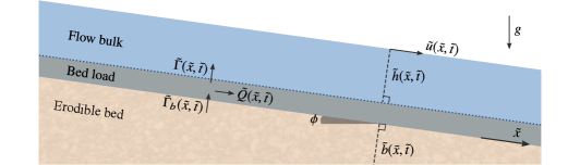
Figure 1: Diagram of the system under consideration. A shallow flowing layer of height $\tilde{h}$ and velocity $\tilde{u}$ travels along an initially uniform slope inclined at an angle $\phi$ to the horizontal. Underneath is a bed of height $\tilde{b}$, composed of homogeneous sediment that may be carried as a distinguished load (of fixed depth) along the bed surface, or entrained into the flow bulk. The material transfer variables are labelled with arrows, to indicate the directions of positive transport.

We fix a coordinate $\tilde{x}$, oriented along the slope, which is inclined at a constant angle $\phi$ to the horizontal. Only motions and spatial variations in the flow fields along this axis are considered. Both the flow height $\tilde{h}(\tilde{x},\tilde{t})$ and bed height $\tilde{b}(\tilde{x},\tilde{t})$ are measured in the direction normal to the slope and the depth of flowing material is everywhere assumed to be small, relative to its streamwise and lateral coverage along the slope plane.

Governing equations for flows in this setting may be obtained by integrating the continuity and momentum transport equations for a general continuum body over the flow depth and neglecting terms that are small for a shallow layer. This standard procedure eliminates both the slope-normal components of motion and any non-hydrostatic pressure gradients, and replaces the downslope velocity with its depth-averaged value, denoted herein by $\tilde{u}(\tilde{x},\tilde{t})$. Allowing for linear-order variations in the bed gradient results in a contribution to the depth-averaged hydrostatic pressure term only. Higher-order variations (i.e. curvatures) may be considered, but these are not relevant for studying the linear stability of flows on constant slopes. For simplicity, we also choose to omit ‘shape factors’ – free parameters arising from the depth integration that quantify the level of vertical shear in the velocity profile. While these can, in certain cases, modify solutions significantly (Hogg & Pritchard, 2004), they are typically unknown and very often neglected in modelling studies (Macedonio & Pareschi, 1992; Iverson, 1997; Cao et al., 2004; Xia et al., 2010, for example). Nevertheless, our analysis could in principle be adapted to include them.

If there are no morphodynamic processes present, the depth-averaged flow density $\tilde{\rho}(\tilde{x},\tilde{t})$ is a constant field and the equations of motion are:

$$\frac{\partial\tilde{h}}{\partial\tilde{t}}+\frac{\partial~{}}{\partial\tilde{x}}\left(\tilde{h}\tilde{u}\right)=0,$$ (1a)

$$\frac{\partial~{}}{\partial\tilde{t}}\left(\tilde{h}\tilde{u}\right)+\frac{\partial~{}}{\partial\tilde{x}}\left(\tilde{h}\tilde{u}^{2}\right)+g\tilde{h}\cos\phi\frac{\partial~{}}{\partial\tilde{x}}\left(\tilde{h}+\tilde{b}\right)=g\tilde{h}\sin\phi-\tilde{\tau}/\tilde{\rho}.$$ (1b)

The final component of (1b) is a forcing term obtained from depth integration of the material stresses. It is a free constitutive law that captures the aggregate rheology of the flow. A typical example is to set $\tilde{\tau}\propto\tilde{u}^{2}$, which models the turbulent drag experienced by a fluid moving over a rough surface, although there are many other choices. To encompass a broad range of systems in our analysis, we take $\tilde{\tau}$ to be an arbitrary function of the local flow fields.

We now allow the flow to exchange fluids and solids with the underlying bed, whose height $\tilde{b}(\tilde{x},t)$ is measured in line with $\tilde{h}$. Entrained solid material is assumed to be composed of homogeneous particles of density $\tilde{\rho}_{s}$ that are much smaller than the flow depth, so that they may be treated as a continuous phase occupying a (depth-averaged) fraction $\tilde{\psi}(\tilde{x},\tilde{t})$ of the flow volume. The remainder of the mixture (occupying fraction $1-\tilde{\psi}$) is fluid of constant density $\tilde{\rho}_{f}$. The overall density of the flow is then

$$\tilde{\rho}=\tilde{\rho}_{f}(1-\tilde{\psi})+\tilde{\rho}_{s}\tilde{\psi}.$$ (2)

The volumetric flux of net mass (comprising both fluid and solid phases) transferred to the flow bulk from below shall be denoted by $\tilde{\Gamma}(\tilde{x},\tilde{t})$. This function encapsulates the competing processes of sediment entrainment and deposition into a single source term. (Example parametrisations of these processes are given later, in §4.1.) When $\tilde{\Gamma}>0$, there is net uptake of material into the suspended load of the bulk; when $\tilde{\Gamma}<0$, there is a net loss. On including the contribution of this term equation (1a), which describes conservation of the total flow mass, becomes

$$\frac{\partial\tilde{h}}{\partial\tilde{t}}+\frac{\partial~{}}{\partial\tilde{x}}(\tilde{h}\tilde{u})=\tilde{\Gamma}.$$ (3a)

We assume the bed has constant density $\tilde{\rho}_{b}$ and is everywhere saturated, comprising a homogeneous mixture of fluid and solids, with the latter phase occupying volumetric fraction $\tilde{\psi}_{b}$. The volumetric flux of the solid and fluid phases into the flow bulk are then necessarily $\tilde{\psi}_{b}\tilde{\Gamma}$ and $(1-\tilde{\psi}_{b})\tilde{\Gamma}$ respectively. This leads to a separate mass conservation equation for the solid phase:

$$\frac{\partial~{}}{\partial\tilde{t}}(\tilde{\psi}\tilde{h})+\frac{\partial~{}}{\partial\tilde{x}}(\tilde{\psi}\tilde{h}\tilde{u})=\tilde{\psi}_{b}\tilde{\Gamma}.$$ (3b)

Between the flowing layer and the bed, we allow for a distinguished mobile layer of material, commonly referred to as the bed load, that travels with flux $\tilde{Q}(\tilde{x},\tilde{t})$. Below this layer, the underlying substrate is assumed to be immobile and transfers material to the bed load at a rate $\tilde{\Gamma}_{b}$, such that the bed height obeys $\partial\tilde{b}/\partial\tilde{t}=-\tilde{\Gamma}_{b}$. If the middle bed load layer possesses a constant characteristic thickness, its mass conservation relation is given by simply $\partial\tilde{Q}/\partial\tilde{x}=\tilde{\Gamma}_{b}-\tilde{\Gamma}$. (Figure 1 is a useful reference for the sign conventions of the fluxes and source terms here.) Therefore, conservation of mass for the moving and immobile components of the bed as a whole implies

$$\frac{\partial\tilde{b}}{\partial\tilde{t}}+\frac{\partial\tilde{Q}}{\partial\tilde{x}}=-\tilde{\Gamma}.$$ (3c)

The inclusion of bed load conceptually separates the gradual crawl of grains along the bed surface (as typically observed in fluvial systems, for example), from transfer of sediment with the bulk flow. The latter process, through changes to the bulk density and drag characteristics, affects the dynamics of the overlying flow. Since these processes are commonly modelled by flux and source terms respectively, they cannot be combined in our analysis.

To complete the morphodynamic description, the momentum conservation equation (1b) must be amended to account for spatial variations in $\tilde{\rho}$ that may arise via the transport dynamics of the solids fraction. Re-deriving (1b) from the morphodynamic standpoint introduces a density dependence into each term and also leads to an extra contribution $\tilde{\rho}\tilde{u}_{b}\tilde{\Gamma}$, included in some models, that accounts for jumps in velocity, stress and density between the flow and the layer beneath it, which necessarily occur when particles are either mobilised or de-entrained. In the absence of bed load, this term represents the rate of change of momentum required to accelerate the entrained material to a characteristic slip velocity $\tilde{u}_{b}(\tilde{h},\tilde{u},\tilde{\psi})$ near the bed surface. A comprehensive derivation and discussion of this term is given by Iverson & Ouyang (2015). The complete governing equation for momentum can be written as

$$\frac{\partial~{}}{\partial\tilde{t}}(\tilde{\rho}\tilde{h}\tilde{u})+\frac{\partial~{}}{\partial\tilde{x}}\left(\tilde{\rho}\tilde{h}\tilde{u}^{2}\right)+\frac{1}{2}g\cos\phi\frac{\partial~{}}{\partial\tilde{x}}\left(\tilde{\rho}\tilde{h}^{2}\right)=\tilde{\rho}g\tilde{h}\left(\sin\phi-\cos\phi\frac{\partial\tilde{b}}{\partial\tilde{x}}\right)-\tilde{\tau}+\tilde{\rho}\tilde{u}_{b}\tilde{\Gamma}.$$ (3d)

Equations (3da–d) constitute a general shallow-water model for a sediment-carrying flow, coupled with its underlying topography by closures for mass exchange and bed load flux. Our goal is to understand some of the general properties of these models, the solutions of the governing equations and their stability. We divide this overall framework into four subcategories:

1. Hydraulic limit. When $\tilde{\Gamma}=\tilde{Q}=0$, (3da–d) reduce to equations (1a,b), which are appropriate for flows on inerodible substrates. These have been thoroughly studied elsewhere and provide a useful reference point for the other cases. We briefly cover their linear stability in §3.1.

2. Suspended load model. When $\tilde{\Gamma}\neq 0$ and $\tilde{Q}=0$, any eroded sediment is entrained directly into the bulk flow. This is our primary focus in the paper. Models in this class are employed to describe energetic flows with significant sediment uptake and mixing, often leading to high solids concentrations. Recent example studies from the literature include (but are not limited to) Cao et al. (2004, 2006); Wu & Wang (2007); Yue et al. (2008) and Li & Duffy (2011). We derive general linear stability results for these models in §3.2 and §3.3; existence of steady solutions and their stability properties are explored in detail for an example model in §4.2–§4.6.

3. Bed load model. When $\tilde{\Gamma}=0$ and $\tilde{Q}\neq 0$, eroded sediment is only carried in the distinguished bed load layer. These models are most often used in fluvial settings, where the effects of lateral sediment transport are important, but individual grains receive little upward momentum and remain largely near the bed surface. These models are widely used: a partial list of examples in the literature includes Hudson & Sweby (2005); Murillo & García-Navarro (2010); Benkhaldoun et al. (2011); Siviglia et al. (2013); Juez et al. (2014); Kozyrakis et al. (2016).

4. Combined model. A few recent studies allow for both $\tilde{\Gamma}\neq 0$ and $\tilde{Q}\neq 0$, including Wu & Wang (2007); Liu et al. (2015); Liu & Beljadid (2017) and a two-layer model due to Swartenbroekx et al. (2013) (which includes a momentum equation for the bed load layer and is therefore not strictly encompassed herein). This is approach is less commonplace, but potentially useful for physical situations that fall between the regimes of (ii) and (iii). Moreover, as we suggest below, it may be more widely applicable as a way to address issues with the formulation of suspended load models. We analyse the well posedness of these models together with pure bed load models in §3.4. Existence of steady states for example closures in the combined model is analysed in §4.2 and their linear stability is explored in §4.7.

While very many models fit our general framework, there are a few underlying assumptions that are important to list, since they dictate the scope of our analysis. We have already made explicit our requirement that the flow and bed are composed of small, roughly homogeneous grains, so that the solid fraction may be treated as a single continuous phase. Moreover, we have neglected the equations for bed load momentum (usually considered negligible) and the solid phase momentum, which may be combined with that of the overall mixture provided the flow is well mixed. Amongst other physical effects, we have implicitly neglected the role of interstitial pore fluid pressures between grains, whose dynamics couples with shear and dilation of the granular phase (Guazzelli & Pouliquen, 2018). These interacting processes can lead to dramatic transients known to impact flow outcomes and cause debris flows to be sensitive to initiation conditions (Iverson, 1997; Iverson et al., 2000). Consequently, our analysis is only strictly relevant to flow regimes where pore pressure is negligible (i.e. less concentrated flows), or situations where the system has everywhere relaxed to the ambient hydrostatic pressure.

3 Linear stability

We assume the presence of a uniform steady flowing layer of height $\tilde{h}_{0}$, velocity $\tilde{u}_{0}$, solid fraction $\tilde{\psi}_{0}$, density $\tilde{\rho}_{0}=\tilde{\rho}(\tilde{\psi}_{0})$, travelling on a flat sloping bed of (arbitrary) height $\tilde{b}_{0}$. According to (3da–d), the existence of such a solution depends on the particular parametrisations for drag and solids exchange, which must satisfy

$$\tilde{\tau}(\tilde{h}_{0},\tilde{u}_{0},\tilde{\psi}_{0})=\tilde{\rho}_{0}g\tilde{h}_{0}\sin\phi~{}~{}\mathrm{and}~{}~{}\tilde{\Gamma}(\tilde{h}_{0},\tilde{u}_{0},\tilde{\psi}_{0})=0.$$ (4a,b)

That is, at steady state, gravitational forcing is exactly balanced by the basal drag and there is no net mass transfer between the bed and the flow. We may linearise the governing equations around these putative steady flows without making explicit choices for $\tilde{\tau}$ and $\tilde{\Gamma}$. The bed load $\tilde{Q}$ may also be kept as a general unknown function. In doing so, we obtain general expressions that can be adapted to different situations by inputting appropriate closures. Detailed discussion of the existence of steady flows, specialised to the case of fluid–grain mixtures, is given later, in §4.2.

For simplicity, we choose to rescale length, time and the dynamical variables as

$$x=\tilde{x}/\tilde{\ell}_{0},~{}t=\tilde{t}\tilde{u}_{0}/\tilde{\ell}_{0},~{}h=\tilde{h}/\tilde{h}_{0},~{}u=\tilde{u}/\tilde{u}_{0},~{}\psi=\tilde{\psi}/\tilde{\psi}_{b}~{}\text{and}~{}b=\tilde{b}/\tilde{h}_{0},$$ (5a–f)

where $$\tilde{\ell}_{0}\equiv\tilde{u}_{0}^{2}/(g\sin\phi)$$. Additionally, we define

$$\tau=\tilde{\tau}/\tilde{\tau}_{0},~{}\Gamma=\tilde{\Gamma}\tilde{\ell}_{0}/(\tilde{h}_{0}\tilde{u}_{0}),~{}Q=\tilde{Q}/(\tilde{h}_{0}\tilde{u}_{0}),~{}u_{b}=\tilde{u}_{b}/\tilde{u}_{0},~{}\rho=\tilde{\rho}/\tilde{\rho}_{0},~{}\mathrm{and}~{}\rho_{i}=\tilde{\rho}_{i}/\tilde{\rho}_{0},$$ (5g–l)

for $\tilde{\rho}_{i}\in\{\tilde{\rho}_{b},\tilde{\rho}_{f},\tilde{\rho}_{s}\}$ and $\tilde{\tau}_{0}\equiv\tilde{\rho}_{0}g\tilde{h}_{0}\sin\phi$. On substituting (5a–l) into the governing equations (3da–d) and simplifying, one arrives at

$$\frac{\partial h}{\partial t}+\frac{\partial~{}}{\partial x}(hu) =\Gamma,$$ (6a)

$$\frac{\partial~{}}{\partial t}(\psi h)+\frac{\partial~{}}{\partial x}(\psi hu) =\Gamma,$$ (6b)

$$\frac{\partial~{}}{\partial t}(\rho hu)+\frac{\partial~{}}{\partial x}\left(\rho hu^{2}+\frac{1}{2}\mbox{{Fr}}^{-2}\rho h^{2}\right) =\rho h\left(1-\mbox{{Fr}}^{-2}\frac{\partial b}{\partial x}\right)-\tau+\rho u_{b}\Gamma,$$ (6c)

$$\frac{\partial b}{\partial t}+\frac{\partial Q}{\partial x} =-\Gamma,$$ (6d)

where $\mbox{{Fr}}\equiv\tilde{u}_{0}/(g\tilde{h}_{0}\cos\phi)^{1/2}$ is the Froude number of the steady flow.

In this rescaled problem, the steady flow is a solution of (6a)–(6d) with height $h_{0}=1$, velocity $u_{0}=1$, solid fraction $\psi_{0}=\tilde{\psi}_{0}/\tilde{\psi}_{b}$ and arbitrary bed height $b_{0}$. The density of the layer is $\rho_{0}=1$. Any slope-aligned perturbation to this state may be decomposed into individual Fourier modes of real wavenumber $k$, which grow or decay in time at some unknown complex growth rate $\sigma$. To find a general formula for $\sigma$, we construct the following ansatz:

$$h(x,t)=1+\epsilon h_{1}\exp(\sigma t+\mathrm{i}\mkern 1.0mukx),$$ (7a)

$$u(x,t)=1+\epsilon u_{1}\exp(\sigma t+\mathrm{i}\mkern 1.0mukx),$$ (7b)

$$\psi(x,t)=\psi_{0}+\epsilon\psi_{1}\exp(\sigma t+\mathrm{i}\mkern 1.0mukx),$$ (7c)

$$b(x,t)=b_{0}+\epsilon b_{1}\exp(\sigma t+\mathrm{i}\mkern 1.0mukx),$$ (7d)

where $h_{1},u_{1},\psi_{1},b_{1}$ are unknown constants and $\epsilon\ll 1$. By substituting (7a)–(7d) into (6a–d) and dropping $O(\epsilon^{2})$ terms, we obtain a linear system of the form

$$\sigma\mathsfbi{A}\boldsymbol{q}+\mathrm{i}\mkern 1.0muk\mathsfbi{B}\boldsymbol{q}+\mathsfbi{C}\boldsymbol{q}=\boldsymbol{0},$$ (8)

where $\boldsymbol{q}=(h_{1},u_{1},\psi_{1},b_{1})^{T}$, and $\mathsfbi{A}$, $\mathsfbi{B}$, $\mathsfbi{C}$ are $4\times 4$ matrices, defined shortly. This is a generalised eigenvalue problem for $\sigma(k)$. For each wavenumber, it has four solutions, whose eigenvectors $\boldsymbol{q}(k)$ correspond, via (7a)–(7d), to disturbance amplitudes that grow exponentially with rate $\Real(\sigma)$ and travel along the slope at wave speed $c=-\Imag(\sigma)/k$. Instability occurs when any of these solutions exponentially diverges from the steady state, i.e. when $\Real[\sigma(k)]>0$. The matrices are:

$$\mathsfbi{A}=\begin{pmatrix}1&0&0&0\\ \psi_{0}&0&1&0\\ 1&1&\Delta\rho&0\\ 0&0&0&1\\ \end{pmatrix},\quad\mathsfbi{B}=\begin{pmatrix}1&1&0&0\\ \psi_{0}&\psi_{0}&1&0\\ 1+\mbox{{Fr}}^{-2}&2&\Delta\rho(1+\frac{1}{2}\mbox{{Fr}}^{-2})&\mbox{{Fr}}^{-2}\\ Q_{h_{0}}&Q_{u_{0}}&Q_{\psi_{0}}&0\\ \end{pmatrix}$$ (9a,b)

and

$$\mathsfbi{C}=\begin{pmatrix}-\Gamma_{h_{0}}&-\Gamma_{u_{0}}&-\Gamma_{\psi_{0}}&0\\ -\Gamma_{h_{0}}&-\Gamma_{u_{0}}&-\Gamma_{\psi_{0}}&0\\ \tau_{h_{0}}-1-\upsilon_{0}\Gamma_{h_{0}}&\tau_{u_{0}}-\upsilon_{0}\Gamma_{u_{0}}&\tau_{\psi_{0}}-\Delta\rho-\upsilon_{0}\Gamma_{\psi_{0}}&0\\ \Gamma_{h_{0}}&\Gamma_{u_{0}}&\Gamma_{\psi_{0}}&0\\ \end{pmatrix}.$$ (9c)

For the sake of neatness, we have used some notational shorthand to simplify the entries. In particular, we set $\Delta\rho\equiv\tilde{\psi}_{b}(\rho_{s}-\rho_{f})$, so that

$$\rho(\psi)=\rho_{f}+\Delta\rho\psi,$$ (10)

by (2) and (5e,k,l). The matrices $\mathsfbi{B}$ and $\mathsfbi{C}$ depend on linear expansions of the unknown functions $Q$, $\tau$ and $\Gamma$ around the steady state. In these cases, we have written $f_{\zeta_{0}}\equiv\frac{\partial f}{\partial\zeta}\big{|}_{1,1,\psi_{0}}$ for each $f\in\{Q,\tau,\Gamma\}$ and $\zeta\in\{h,u,\psi,b\}$. Note that, in deriving $\mathsfbi{B}$ and $\mathsfbi{C}$, our assumption of a homogeneous bed allowed us to set $Q_{b_{0}}=\tau_{b_{0}}=\Gamma_{b_{0}}=0$. Finally, the basal slip velocity, evaluated at the steady state, is denoted as $\upsilon_{0}\equiv u_{b}(1,1,\psi_{0},b_{0})$.

3.1 Hydraulic limit

We begin our analysis by briefly recapping the ‘purely hydraulic’ stability problem within our framework. That is, we address the limiting case of weak morphodynamic processes, by sending both $Q\to 0$ and $\Gamma\to 0$. In this case, perturbations in $\psi$ and $b$ can only be advected along the slope, since there are no morphodynamic feedbacks through which they may grow or decay. Equation (8) possesses the solutions $\sigma=-\mathrm{i}\mkern 1.0muk$ and $\sigma=0$, that respectively correspond to these modes of disturbance. The remaining two solutions are

$$\sigma=-\mathrm{i}\mkern 1.0muk-\frac{\tau_{u_{0}}}{2}\pm\sqrt{\tau_{u_{0}}^{2}/4-k^{2}/\mbox{{Fr}}^{2}+\mathrm{i}\mkern 1.0muk(\tau_{h_{0}}-1)}.$$ (11)

These branches correspond to disturbances in the hydraulic governing equations for $h$ and $u$, studied in the case of general drag by Trowbridge (1987). When $k=0$, they pass through $\sigma=-\tau_{u_{0}}$ and $0$. It can be shown straightforwardly that $\Real(\sigma)$ is a monotonic function with respect to $|k|$, meaning that the maximum growth for each branch must occur at either $k=0$, or in the limit $|k|\to\infty$. Growth rate saturation at short wavelengths is a known property of the classical roll wave instability that highlights the omission of physics (turbulent dissipation) that would otherwise damp out disturbances over short length scales. Evaluating the limit of (11) as $|k|\to\infty$ yields

$$\Real(\sigma)\to\frac{-\tau_{u_{0}}\pm|1-\tau_{h_{0}}|\mbox{{Fr}}}{2}.$$ (12)

If $\tau_{u_{0}}<0$, then there is always unstable growth (i.e. at $k=0$). However, we consider the more physically reasonable situation where $\tau_{u_{0}}>0$ (i.e. a drag parametrisation that increases resistance to flow at higher shear rates). Then, if $\tau_{h_{0}}=1$, both branches are everywhere stable and asymptote to $\Real(\sigma)=-\tau_{u_{0}}/2$. Otherwise, since the argument of the square root in (11) always has a non-zero imaginary part (away from $k=0$), the growth rates are always distinct and in particular, the branch with positive root always dominates. This turns unstable when (12) exceeds zero, which occurs if

$$\mbox{{Fr}}>\frac{\tau_{u_{0}}}{|1-\tau_{h_{0}}|}.$$ (13)

This is the stability criterion due to Trowbridge (1987), written in our dimensionless quantities. Inclusion of the absolute value in the denominator constitutes a minor correction to the original formula that accounts for the case where $\tau_{h_{0}}>1$.

3.2 Suspended load model

We now reintroduce morphodynamics, by allowing for non-vanishing mass exchange with the bed ($\Gamma\neq 0$), but continuing to neglect bed load transport ($Q=0$). This substantially complicates (8), which becomes a fully $4\times 4$ problem. Motivated by the above discussion, we divide our morphodynamic analysis into two tractable regimes: the long-wave (or global) limit $k=0$ and the short-wave limit $k\gg 1$, and verify later that these limits control most of the important aspects of the problem.

3.2.1 Global modes: $k=0$

A given steady morphodynamic flow is specified by four state variables $\tilde{h}_{0}$, $\tilde{u}_{0}$, $\tilde{\psi}_{0}$ and $\tilde{b}_{0}$, which are constrained by only two equations (4a,b). Therefore, the solution space is underdetermined and there is a two-dimensional linear family of possible steady states. In nature, selection of a particular flow from this family is assured via some boundary condition, such as the total flux of material through a flow cross-section. Moreover, transitions from one steady flow to another within this space can occur (through an increase in the total flux). Infinitesimal transitions between steady states are linear perturbations in the sense of (7a)–(7d), with $k=0$ and $\sigma=0$ (neutral stability). Therefore, by (8) they satisfy $\mathsfbi{C}\boldsymbol{q}=\boldsymbol{0}$. Solving for $\boldsymbol{q}$ reveals a two-dimensional space of neutral modes spanned by

$$\boldsymbol{v}_{1}=\begin{pmatrix}(\tau_{\psi_{0}}-\Delta\rho)\Gamma_{u_{0}}-\tau_{u_{0}}\Gamma_{\psi_{0}}\\ (\Delta\rho-\tau_{\psi_{0}})\Gamma_{h_{0}}+(\tau_{h_{0}}-1)\Gamma_{\psi_{0}}\\ \tau_{u_{0}}\Gamma_{h_{0}}-(\tau_{h_{0}}-1)\Gamma_{u_{0}}\\ 0\end{pmatrix},\quad\boldsymbol{v}_{2}=\boldsymbol{e}_{4},$$ (14a,b)

where we adopt the convention of using $\boldsymbol{e}_{j}$ to denote the $j$-th standard basis vector. The first of these, $\boldsymbol{v}_{1}$, may be interpreted in the following way. Written in our dimensionless variables, the equations for steady flows (4a,b) are the roots of the function $\boldsymbol{F}(h,u,\psi)=(\tau-\rho h,\Gamma)^{T}$. It is straightforward to verify that $\nabla\boldsymbol{F}(h_{0},u_{0},\psi_{0})\cdot\boldsymbol{v}_{1}=\boldsymbol{0}$ and therefore $\boldsymbol{v}_{1}$ represents a shift along the curve of solutions, implicitly defined by $\boldsymbol{F}=\boldsymbol{0}$. The second neutral mode $\boldsymbol{v}_{2}$ accounts for invariance to arbitrary translations of the bed height.

The remaining two global modes have non-zero growth rate and therefore, by (8), they obey

$$\sigma\mathsfbi{A}\boldsymbol{q}+\mathsfbi{C}\boldsymbol{q}=\boldsymbol{0}.$$ (15)

After factoring out the neutral growth rates, the characteristic equation yields a quadratic from which the remaining two eigenvalues may be directly computed. The full set of eigenvalues of (15) is then

$$\sigma=0~{}\mathrm{(repeated)},\quad\frac{s_{0}\pm\sqrt{s_{c}}}{2},$$ (16a,b)

where $s_{0}$, $s_{c}$ are placeholders for

$$s_{0}=-\tau_{u_{0}}+\Gamma_{h_{0}}+(\upsilon_{0}-\rho_{b})\Gamma_{u_{0}}+(1-\psi_{0})\Gamma_{\psi_{0}},$$ (17a)

$$\begin{aligned} s_{c}=\Gamma_{u_{0}}^{2}(\upsilon_{0}-\rho_{b})^{2}+2\Gamma_{u_{0}}\left\{(\upsilon_{0}-\rho_{b})\left[\Gamma_{h_{0}}+(1-\psi_{0})\Gamma_{\psi_{0}}-\tau_{u_{0}}\right]\right.\\ \left.-2\left[\tau_{h_{0}}+\tau_{\psi_{0}}(1-\psi_{0})-\rho_{b}\right]\right\}+\left[\tau_{u_{0}}+\Gamma_{h_{0}}+(1-\psi_{0})\Gamma_{\psi_{0}}\right]^{2}\!\!.\end{aligned}$$ (17b)

Here, we have made use of (10) with $\psi=\psi_{0}$ and $\psi=\psi_{b}=1$, to eliminate $\Delta\rho$ in favour of the bed density $\rho_{b}=1+\Delta\rho(1-\psi_{0})$ in these expressions, which nevertheless depend on all nine independent quantities in the matrices $\mathsfbi{A}$ and $\mathsfbi{C}$. Before moving on to the next section, we note two important special cases.

In the non-erosive limit $\Gamma\to 0$, (17a) and (17b) reduce to simply $s_{0}=-\tau_{u_{0}}$ and $s_{c}=\tau_{u_{0}}^{2}$. Substituting these into (16b) leaves only one (typically negative) non-zero growth rate, $\sigma=-\tau_{u_{0}}$, consistent with the analysis in §3.1.

If instead, $\Gamma$ is finite, but $|\Gamma_{u_{0}}|$ is sufficiently small, relative to the other components of (17a,b), so that it may be neglected, the non-zero eigenvalues become

$$\sigma=\frac{s_{0}-\sqrt{s_{c}}}{2}=-\tau_{u_{0}}~{}~{}\mathrm{and}~{}~{}\sigma=\frac{s_{0}+\sqrt{s_{c}}}{2}=\Gamma_{h_{0}}+\Gamma_{\psi_{0}}(1-\psi_{0}).$$ (18a,b)

Since the latter eigenvalue (later referred to as $\sigma_{a}$) may be positive, there exists a route to a purely morphodynamic instability in this case, which depends on the signs and relative magnitudes of $\Gamma_{h_{0}}$ and $\Gamma_{\psi_{0}}$. Positive values for these derivatives imply positive morphodynamic feedbacks, amplifying the flow depth and concentration respectively. We return to this in §4, where we demonstrate using some generic model closures that this mode can indeed be unstable.

3.2.2 Short wavelengths: $k\gg 1$

We now focus on short-wavelength perturbations. By analogy with the non-morphodynamic case of §3.1, we anticipate that the limit $k\to\infty$ controls the onset and growth of instabilities by maximising $\Real[\sigma(k)]$. (We confirm that this is often the case for example model closures in §4.) The form of (8) suggests the following asymptotic expansions for the four growth rates and their corresponding eigenmodes in this regime:

$$\sigma=-\mathrm{i}\mkern 1.0mu\lambda_{1}k+\lambda_{0}+\lambda_{-1}k^{-1}+\ldots,\quad\boldsymbol{q}=\boldsymbol{q}_{0}+\boldsymbol{q}_{-1}k^{-1}+\ldots$$ (19a,b)

Here, $\lambda_{1}$, $\lambda_{0}$, $\lambda_{-1}$ and $\boldsymbol{q}_{0}$, $\boldsymbol{q}_{-1}$, are unknown constants and vectors to be determined shortly. Substituting these expressions into (8) and retaining only the leading $O(k)$ terms leaves an eigenproblem for $\lambda_{1}$:

$$\lambda_{1}\mathsfbi{A}\boldsymbol{q}_{0}=\mathsfbi{B}\boldsymbol{q}_{0}.$$ (20)

This may be solved to obtain four distinct values

$$\lambda_{1}=1\pm\mbox{{Fr}}^{-1},~{}1,~{}0.$$ (21)

Since $c=-\Imag(\sigma)/k\to\lambda_{1}$ as $k\to\infty$, these are the wave speeds for disturbances in the short-wavelength regime (and also the characteristics of the governing equations in this context). The corresponding eigenvectors of (20) are

$$\boldsymbol{q}_{0}=\begin{pmatrix}\pm\mbox{{Fr}}\\ 1\\ 0\\ 0\end{pmatrix},~{}\begin{pmatrix}\Delta\rho/2\\ 0\\ -1\\ 0\end{pmatrix},~{}\begin{pmatrix}1\\ -1\\ 0\\ \mbox{{Fr}}^{2}-1\end{pmatrix}.$$ (22)

Recalling the definition $\boldsymbol{q}=(h_{1},u_{1},\psi_{1},b_{1})^{T}$ and (7a)–(7d), the elements of these vectors are the leading-order amplitudes for each mode. Throughout the rest of the paper, we label these modes I–IV. Since these asymptotic vectors separate the four solution branches of the general linear problem (8), it will be convenient later to use the same labels to refer to quantities at finite $k$, though they may not necessarily share the properties of their asymptotic counterparts.

The first pair of modes (I,II) in (22) contain no morphodynamic content. Indeed, they are identical to the short-wavelength modes of the purely hydraulic problem (§3.1), which is guaranteed since $\mathsfbi{A}$ and $\mathsfbi{B}$ do not depend on $\Gamma$. They describe disturbances in $h$ and $u$, propagating at speeds $c=1\pm\mbox{{Fr}}^{-1}$. Mode III couples unit speed perturbations in $\psi$ with the flow free surface, while mode IV is stationary ($c=0$) and disturbs the bedform, as well as $h$ and $u$.

The second term in the expansion of $\sigma$ determines the leading-order real part of the growth rate. We substitute (19a,b) back into (8) and subtract away the $O(k)$ component, i.e. (20). Retaining only $O(1)$ terms in the remaining equation, leaves

$$\lambda_{0}\mathsfbi{A}\boldsymbol{q}_{0}+\mathrm{i}\mkern 1.0mu(\mathsfbi{B}-\lambda_{1}\mathsfbi{A})\boldsymbol{q}_{-1}=\mathsfbi{C}\boldsymbol{q}_{0}.$$ (23)

The unknown vector $\boldsymbol{q}_{-1}$ can be eliminated by solving the eigenproblem adjoint to (20), which yields vectors $\boldsymbol{r}_{0}$ such that $\lambda_{1}\boldsymbol{r}_{0}^{T}\mathsfbi{A}=\boldsymbol{r}_{0}^{T}\mathsfbi{B}$. Multiplying (23) on the left by $\boldsymbol{r}_{0}^{T}$ and rearranging gives the formula

$$\lambda_{0}=-\frac{\boldsymbol{r_{0}}\cdot\mathsfbi{C}\boldsymbol{q}_{0}}{\boldsymbol{r}_{0}\cdot\mathsfbi{A}\boldsymbol{q}_{0}}.$$ (24)

Using this, the following four expressions for $\lambda_{0}$ are obtained, which we label $\lambda_{0,1},\ldots,\lambda_{0,4}$ for later reference:

$$\lambda_{0,1}=\frac{f_{+}(\mbox{{Fr}})}{\mbox{{Fr}}(\mbox{{Fr}}+1)},\quad\lambda_{0,2}=\frac{f_{-}(\mbox{{Fr}})}{\mbox{{Fr}}(\mbox{{Fr}}-1)},$$ (25a,b)

$$\lambda_{0,3}=(1-\psi_{0})(\Gamma_{\psi_{0}}-\Delta\rho\Gamma_{h_{0}}/2),\quad\lambda_{0,4}=\frac{\Gamma_{u_{0}}-\Gamma_{h_{0}}}{\mbox{{Fr}}^{2}-1}.$$ (25c,d)

By (19a), these asymptotic values dictate the limits of $\Real(\sigma)$ as $k\to\infty$ for modes I–IV. We list them in the same order as their respective wave speeds in (21) and the $O(1)$ eigenvectors in (22). The functions $f_{\pm}$ are third-order polynomials in Fr defined by

$$\begin{aligned} f_{\pm}(\mbox{{Fr}})=&\pm\frac{1}{2}\left[\Gamma_{h_{0}}(\upsilon_{0}-\rho_{b})+(1-\tau_{h_{0}})\right]\mbox{{Fr}}^{3}\\ &+\frac{1}{2}\left[\Gamma_{h_{0}}(2\upsilon_{0}-\rho_{b}+1)/2+\Gamma_{u_{0}}(\upsilon_{0}-\rho_{b})+1-\tau_{h_{0}}-\tau_{u_{0}}\right]\mbox{{Fr}}^{2}\\ &\pm\frac{1}{4}\left[\Gamma_{h_{0}}(\rho_{b}-1)+\Gamma_{u_{0}}(2\upsilon_{0}-\rho_{b}+1)-2\tau_{u_{0}}\right]\mbox{{Fr}}+\frac{1}{4}\Gamma_{u_{0}}(\rho_{b}-1).\end{aligned}$$ (26)

It is easily confirmed that as $\Gamma\to 0$, $\lambda_{0,1}$ and $\lambda_{0,2}$ reduce to the high-$k$ growth rates of the non-erosive problem, given in (12), while $\lambda_{0,3},\lambda_{0,4}\to 0$. For this reason, we will sometimes label $\lambda_{0,1}$, $\lambda_{0,2}$ and their corresponding modes (I,II) as ‘hydraulic’ and $\lambda_{0,3}$, $\lambda_{0,4}$ as ‘morphodynamic’ even though all of (25a–d) are coupled to the bed and sediment dynamics when $\Gamma$ is non-vanishing.

Just as in the non-erosive problem, the asymptotic growth rates in (25a–d) are non-zero, but typically finite. However, there is an extra complication. Since $f_{\pm}(0)=\Gamma_{u_{0}}(\rho_{b}-1)/4$ and $f_{\pm}(\mp 1)=(\Gamma_{h_{0}}-\Gamma_{u_{0}})/2$, the pairs $(\lambda_{0,1},\lambda_{0,2})$ and $(\lambda_{0,2},\lambda_{0,4})$ possess singularities at $\mbox{{Fr}}=0$ and $\mbox{{Fr}}=1$ respectively (provided $\Gamma_{h_{0}}\neq\Gamma_{u_{0}}\neq 0$).

When $\mbox{{Fr}}=0$, the steady flow velocity is zero. The singularities in the expressions for $\lambda_{0,1}$ and $\lambda_{0,2}$ are artefacts arising from the fact that the time scale chosen to non-dimensionalise (6a–d) vanishes in the limit $\tilde{u}_{0}\to 0$. Referring back to (5b,h,l), we may rewrite (25a,b) in dimensional units and verify that these growth rates remain finite. Specifically, when $\tilde{u}_{0}=0$, the expressions are $\tilde{\lambda}_{0,j}=(3/4-j/2)\tilde{\Gamma}_{\tilde{u}_{0}}(\tilde{\rho}_{b}/\tilde{\rho}_{0}-1)(g\cos\phi/\tilde{h}_{0})^{1/2}$, for $j=1,2$.

However, the singularities in (25b,d) at unit Froude number cannot be removed by a choice of units. They occur when the wave speeds $\lambda_{1}=1-\mbox{{Fr}}^{-1},0$ for disturbances to the flow and bedform, coalesce, as do the corresponding $O(1)$ modes in (22). Since $\lambda_{0}$ cannot be $O(1)$ at this singular point, our expansions in (19a,b) are inappropriate here. Therefore, we propose instead that at $\mbox{{Fr}}=1$ (and for modes II & IV only), $\sigma$ and $\boldsymbol{q}$ take the asymptotic form

$$\sigma=\lambda_{1/2}k^{1/2}+\lambda_{0}+\ldots,\quad\boldsymbol{q}=\boldsymbol{q}_{0}+\boldsymbol{q}_{-1/2}k^{-1/2}+\boldsymbol{q}_{-1}k^{-1}+\ldots,$$ (27a,b)

where $\lambda_{1/2}$, $\lambda_{0}$ and $\boldsymbol{q}_{0}$, $\boldsymbol{q}_{-1/2}$, $\boldsymbol{q}_{-1}$ are to be determined. We proceed as before, by substituting these expressions into (8) and isolating its constituent parts at different orders in $k$. Retaining only $O(k)$ terms yields $\mathsfbi{B}\boldsymbol{q}_{0}=0$, with only one solution, $\boldsymbol{q}_{0}=(1,-1,0,0)^{T}$. As it must, this matches the coalescent modes in (22), when they are evaluated at $\mbox{{Fr}}=1$. At $O(k^{1/2})$, we have

$$\lambda_{1/2}\mathsfbi{A}\boldsymbol{q}_{0}+\mathrm{i}\mkern 1.0mu\mathsfbi{B}\boldsymbol{q}_{-1/2}=0.$$ (28)

On substituting $\boldsymbol{q}_{0}$ into this equation, a little algebra shows that $\boldsymbol{e}_{4}\cdot\boldsymbol{q}_{-1/2}=2\mathrm{i}\mkern 1.0mu\lambda_{1/2}$. To find $\lambda_{1/2}$, we use the $O(1)$ equation, which is

$$\lambda_{0}\mathsfbi{A}\boldsymbol{q}_{0}+\lambda_{1/2}\mathsfbi{A}\boldsymbol{q}_{-1/2}+\mathrm{i}\mkern 1.0mu\mathsfbi{B}\boldsymbol{q}_{-1}+\mathsfbi{C}\boldsymbol{q}_{0}=\boldsymbol{0}.$$ (29)

Now we notice that $\boldsymbol{e}_{4}\cdot\mathsfbi{A}\boldsymbol{q}_{0}=\boldsymbol{e}_{4}\cdot\mathsfbi{B}\boldsymbol{v}=0$ for any vector $\boldsymbol{v}$. Therefore, projecting (29) onto $\boldsymbol{e}_{4}$ eliminates the unknowns $\lambda_{0}$ and $\boldsymbol{q}_{-1}$. On doing this, substituting our expressions for $\boldsymbol{q}_{0}$ and $\boldsymbol{e}_{4}\cdot\boldsymbol{q}_{-1/2}$ from above and rearranging, we find

$$\lambda_{1/2}=\pm\frac{1+\mathrm{i}\mkern 1.0mu}{2}\left(\Gamma_{h_{0}}-\Gamma_{u_{0}}\right)^{1/2}.$$ (30)

Except for the particular case $\Gamma_{h_{0}}=\Gamma_{u_{0}}$ (where there is no singularity in $\lambda_{0,2},\lambda_{0,4}$), these expressions have non-zero real part. Therefore, at $\mbox{{Fr}}=1$ and for $k\gg 1$, the second and fourth modes (22) of the linear stability problem (8) diverge with amplitudes $\sim\exp(\pm A\sqrt{k}t)$, where $A=|\Real(\lambda_{1/2})|$. Crucially, one of these amplitudes is strictly positive and unbounded in the limit $k\to\infty$. This implies that the morphodynamic governing equations (6a–d) at are ill posed as an initial value problem when $\mbox{{Fr}}=1$, because their solutions do not depend continuously on initial data (Joseph & Saut, 1990). Mathematically speaking, this is a direct consequence of the model losing the property of strict hyperbolicity when its characteristic wave speeds (21) intersect. More intuitively, problems arise because over any finite time interval, there are short-wavelength disturbances that grow arbitrarily rapidly, making it impossible for the governing equations to behave in a physically consistent way. This fact has practical consequences beyond the theory of steady flows on constant slopes. Computer simulations of these models (in both one and two spatial dimensions) conducted on complex topographies almost inevitably feature locations where the conditions locally match our problem at unit Froude number and shortwave oscillations can grow catastrophically. Numerical ‘solutions’ in this case may nevertheless look physically reasonable, since spatial discretisation imposes an upper limit on $k$. However, they will not converge as the numerical resolution increases and cannot be relied upon to model real flows.

The essential issue of unbounded growth rates in these models was recognised by Balmforth & Vakil (2012), who studied the stability of a similar, but nonequivalent system: uniform flows eroding at a constant positive rate in the Saint-Venant equations. In the limit of slow erosion, they also observed that the high-wavenumber growth rate of perturbations suffers a singularity at unit Froude number. Moreover, they were able to show that the inclusion of a diffusive term in the momentum dynamics was sufficient to regularise their system. Our more general setting adds dynamic coupling with the solid phase and an arbitrary basal drag parametrisation, thereby demonstrating that the same problem affects a far broader range of shallow morphodynamic flow models. Indeed, it suggests that in any situations close to, but not strictly covered by our framework, it is important to check carefully whether the governing equations are well posed and amend them if necessary. Therefore, we continue with an analysis of how this might be achieved.

3.3 Regularisation

We shall introduce a new term to (6c) in order to quash unbounded growth at small length scales. As noted by Joseph & Saut (1990), ill posedness often signals that there are physical processes missing from a model. In our case, two possible culprits are the shallow-layer approximation and the omission of bed load from the current analysis. We assess the effect of bed load shortly, in §3.4. A particular effect neglected by the assumption of shallow flow is the aggregate loss of horizontal momentum caused by turbulent eddies. This is usually acceptable, since it is only significant at length scales shorter than the flow depth. However, for short waves it is no longer strictly negligible. A simple and common way to include this missing physics is to try to capture it via diffusion-like process. We denote a characteristic eddy viscosity for the flow by $\tilde{\nu}$ and non-dimensionalise by setting $\nu=\tilde{\nu}/(\tilde{u}_{0}\tilde{l}_{0})$. This free parameter sets the scale of the diffusive term $\frac{\partial~{}}{\partial x}(\nu\rho h\frac{\partial u}{\partial x})$, which we add to the right-hand side of (6c). We note that the extra term does not affect the steady uniform layer itself. Similar expressions have been employed elsewhere, as a regularisation term by Balmforth & Vakil (2012) in their analysis and in the shallow-flow models of Simpson & Castelltort (2006); Xia et al. (2010) and Langendoen et al. (2016). Later, in §4.6 we briefly address the implications of adding a similar term to (6b) to encapsulate turbulent sediment diffusivity.

It is unclear a priori whether the eddy viscosity term is sufficient to regularise the ill-posed model equations on its own. Therefore, we must extend the high-wavenumber growth rate analysis of §3.2.2. With the extra term, the linearised system of (8) generalises to

$$\sigma\mathsfbi{A}\boldsymbol{q}+\mathrm{i}\mkern 1.0muk\mathsfbi{B}\boldsymbol{q}+\mathsfbi{C}\boldsymbol{q}=-k^{2}\mathsfbi{D}\boldsymbol{q},$$ (31)

where $\mathsfbi{D}=(D_{ij})$ is a $4\times 4$ matrix with entries $D_{32}=\nu$ and $D_{ij}=0$ otherwise. At high wavenumber, the leading-order component in the linearised momentum equation is given by the new diffusive term itself. Suppose that there is at least one eigenvalue that balances this term. This motivates the following asymptotic expansions for $\sigma$ and $\boldsymbol{q}$ when $k\gg 1$:

$$\sigma=\lambda_{2}k^{2}+\lambda_{1}k+\lambda_{0}+\ldots,\quad\boldsymbol{q}=\boldsymbol{q}_{0}+\boldsymbol{q}_{-1}k^{-1}+\boldsymbol{q}_{-2}k^{-2}+\ldots,$$ (32a,b)

where $\lambda_{2}$, $\lambda_{1}$, $\lambda_{0}$ and $\boldsymbol{q}_{0}$, $\boldsymbol{q}_{-1}$, $\boldsymbol{q}_{-2}$ are to be determined. At $O(k^{2})$, equation (31) reduces to the eigenproblem

$$\lambda_{2}\mathsfbi{A}\boldsymbol{q}_{0}=-\mathsfbi{D}\boldsymbol{q}_{0},$$ (33)

with characteristic equation $-\lambda_{2}^{3}(\lambda_{2}+\nu)=0$. When $\lambda_{2}=-\nu$, it may be easily verified that $\boldsymbol{q}_{0}=\boldsymbol{e}_{2}$. Therefore, the diffusion operator creates one stable eigenvalue $\sigma=-\nu k^{2}+O(k)$ associated with viscous damping of $u$. The remaining three solutions are all $\lambda_{2}=0$ and so in these cases $\sigma$ is determined by a lower order balance. Using (33), the corresponding vector $\boldsymbol{q}_{0}$ is determined up to the eigenspace spanned by $\boldsymbol{e}_{1}$, $\boldsymbol{e}_{3}$ and $\boldsymbol{e}_{4}$.

We shall concentrate on the three eigenvalues with $\lambda_{2}=0$, since the mode with $\lambda_{2}=-\nu$ is always stable at high $k$. Then, at $O(k)$, equation (31) becomes

$$(\lambda_{1}\mathsfbi{A}+\mathrm{i}\mkern 1.0mu\mathsfbi{B})\boldsymbol{q}_{0}=-\mathsfbi{D}\boldsymbol{q}_{-1}.$$ (34)

Note that $\boldsymbol{e}_{j}^{T}\mathsfbi{D}=\boldsymbol{0}$ for $j=1,2,4$, since eddy viscosity appears only in the third row of (31). We can therefore eliminate the unknown $\boldsymbol{q}_{-1}$ in (34) as so

$$\boldsymbol{e}_{j}\cdot(\lambda_{1}\mathsfbi{A}+\mathrm{i}\mkern 1.0mu\mathsfbi{B})\boldsymbol{q}_{0}=\boldsymbol{0},\quad\text{for}~{}j=1,2,4.$$ (35)

Likewise, we can write down the eigenproblem adjoint to (34) as $(\lambda_{1}\mathsfbi{A}+\mathrm{i}\mkern 1.0mu\mathsfbi{B})^{T}\boldsymbol{r}_{0}=-\mathsfbi{D}^{T}\boldsymbol{r}_{-1}$, where $\boldsymbol{r}_{0}$ and $\boldsymbol{r}_{-1}$ are unknown left eigenvectors. We will shortly need the constrained problem, with $\boldsymbol{r}_{-1}$ eliminated as so

$$\boldsymbol{e}_{k}\cdot(\lambda_{1}\mathsfbi{A}+\mathrm{i}\mkern 1.0mu\mathsfbi{B})^{T}\boldsymbol{r}_{0}=\boldsymbol{0},\quad\text{for}~{}k=1,3,4.$$ (36)

Expanding $\boldsymbol{q}_{0}=a_{1}\boldsymbol{e}_{1}+a_{3}\boldsymbol{e}_{3}+a_{4}\boldsymbol{e}_{4}$ in (35) results in a $3\times 3$ eigenvalue problem for the unknowns $a_{1}$, $a_{3}$, $a_{4}$ and $\lambda_{1}$. Its characteristic equation is

$$\lambda_{1}(\lambda_{1}+\mathrm{i}\mkern 1.0mu)^{2}=0.$$ (37)

So $\lambda_{1}=0$ or $-\mathrm{i}\mkern 1.0mu$. In either case, we are forced to proceed further to determine the leading real part of $\sigma$. Therefore, we use the $O(1)$ part of (31), which is (for $\lambda_{2}=0$):

$$(\lambda_{0}\mathsfbi{A}+\mathsfbi{C})\boldsymbol{q}_{0}+(\lambda_{1}\mathsfbi{A}+\mathrm{i}\mkern 1.0mu\mathsfbi{B})\boldsymbol{q}_{-1}=-\mathsfbi{D}\boldsymbol{q}_{-2}.$$ (38)

We shall divide our pursuit of $\lambda_{0}$ according to the value of $\lambda_{1}$.

1. Case: $\lambda_{1}=0$. Solving (35) for the eigenvector yields $\boldsymbol{q}_{0}=\boldsymbol{e}_{4}$. To eliminate, the unknown vectors $\boldsymbol{q}_{-1}$ and $\boldsymbol{q}_{-2}$, from (38), we simply note that $\boldsymbol{e}_{4}^{T}\mathsfbi{B}=\boldsymbol{0}$, since the last row of $\mathsfbi{B}$ is all zeros (when $Q=0$). Therefore, we project (38) onto $\boldsymbol{e}_{4}$ and substitute in $\boldsymbol{q}_{0}$ to give

   $$\lambda_{0}=-\frac{\boldsymbol{e}_{4}\cdot\mathsfbi{C}\boldsymbol{e}_{4}}{\boldsymbol{e}_{4}\cdot\mathsfbi{A}\boldsymbol{e}_{4}}=0.$$ (39)

   Referring back to our expansions (32a,b), this means that there always exists an eigenpair $(\sigma,\boldsymbol{q})$ with $\sigma\to 0$ and $\boldsymbol{q}\to\boldsymbol{e}_{4}$ as $k\to\infty$. Note that this situation corresponds to perturbations of the bedform.

2. Case: $\lambda_{1}=-\mathrm{i}\mkern 1.0mu$. Since this is a repeated root, (35) only determines $\boldsymbol{q}_{0}$ within a two-dimensional subspace. Straightforward algebra gives this simply as $\boldsymbol{q}_{0}=a_{1}\boldsymbol{e}_{1}+a_{3}\boldsymbol{e}_{3}$. Similarly, the corresponding adjoint eigenproblem (36), constrains the left eigenvector $\boldsymbol{r}_{0}$ to lie in the subspace spanned by $\boldsymbol{e}_{1}$ and $\boldsymbol{e}_{2}$. We project (38) onto these vectors, yielding

   $$\boldsymbol{e}_{1}\cdot(\lambda_{0}\mathsfbi{A}+\mathsfbi{C})\boldsymbol{q}_{0}+\mathrm{i}\mkern 1.0mu\boldsymbol{e}_{2}\cdot\boldsymbol{q}_{-1}=0,$$ (40a)

   $$\boldsymbol{e}_{2}\cdot(\lambda_{0}\mathsfbi{A}+\mathsfbi{C})\boldsymbol{q}_{0}+\mathrm{i}\mkern 1.0mu\psi_{0}\boldsymbol{e}_{2}\cdot\boldsymbol{q}_{-1}=0.$$ (40b)

   Note that only the second element of $\boldsymbol{q}_{-1}$ appears in these equations. To eliminate it, we return to the full $O(k)$ problem. Since $\boldsymbol{e}_{3}\cdot\mathsfbi{D}\boldsymbol{v}=\nu\boldsymbol{e}_{2}\cdot\boldsymbol{v}$ for any vector $\boldsymbol{v}$, we project (34) onto $\boldsymbol{e}_{3}$ and rearrange to give $\boldsymbol{e}_{2}\cdot\boldsymbol{q}_{-1}=-\mathrm{i}\mkern 1.0mu(2a_{1}+\Delta\rho a_{3})/(2\nu\mbox{{Fr}}^{2})$. Substituting this expression into (40a,b) yields a $2\times 2$ system for $a_{1}$, $a_{3}$ and $\lambda_{0}$, which we solve to find the two eigenvalues

   $$\lambda_{0}=\lambda_{\pm}(\mbox{{Fr}})\equiv\frac{R}{2}+\frac{\pm\sqrt{S}-1}{2\nu\mbox{{Fr}}^{2}},$$ (41)

   where $R\equiv\Gamma_{h_{0}}+\Gamma_{\psi_{0}}(1-\psi_{0})$ and $S\equiv(R\nu\mbox{{Fr}}^{2}+1)^{2}-2\nu\mbox{{Fr}}^{2}\Gamma_{h_{0}}(\rho_{b}+1)$. One of the pair, $\lambda_{-}$, possesses a singularity at $\mbox{{Fr}}=0$. However, as in §3.2.2, this is merely an artefact of our choice of dimensionless units that may be removed by an appropriate rescaling. The corresponding eigenvectors are

   $$\boldsymbol{q}_{0}=\boldsymbol{e}_{1}+\frac{\nu\mbox{{Fr}}^{2}(R-2\Gamma_{h_{0}})+1\pm\sqrt{S}}{2\Gamma_{\psi_{0}}\nu\mbox{{Fr}}^{2}-\Delta\rho}\boldsymbol{e}_{3}.$$ (42)

   In the limit of vanishing eddy viscosity ($\nu\to 0$), $\boldsymbol{q}_{0}\to\boldsymbol{e}_{1}-(1\pm 1)\boldsymbol{e}_{3}/\Delta\rho$. Therefore, since we anticipate small $\nu$, $\lambda_{-}$ corresponds largely to growth in $h$ only, whereas $\lambda_{+}$ corresponds to coupled growth in $h$ and $\psi$. By comparing with the modes of the unregularised problem in (22), $\lambda_{-}$ may be traced to the hydraulic modes and $\lambda_{+}$ to the third mode related to solid fraction perturbations. The former is responsible for very strong damping, since $\lambda_{-}\approx-1/\nu\mbox{{Fr}}^{2}$ for small $\nu$. Conversely, using l’Hôpital’s rule, it may further be verified that $\lim_{\nu\to 0}\lambda_{+}=\lambda_{0,3}$ from (25c). Therefore, in the limit of small $\nu$, this mode is not affected by the regularisation term.

To recap, using (32a,b)–(42), we have computed the growth rates $\sigma$ of perturbations for non-zero values of $\nu$ at leading-order for large wavenumber. These expressions are valid for all $\mbox{{Fr}}>0$ and models of the form (31). They are

$$\sigma=-\nu k^{2}+O(k),\quad 0+O(k^{-1}),\quad-\mathrm{i}\mkern 1.0muk+\lambda_{\pm}(\mbox{{Fr}})+O(k^{-1}),$$ (43a–c)

where $\lambda_{\pm}(\mbox{{Fr}})$ was defined in (41). The corresponding mode amplitudes are given by $\boldsymbol{q}_{0}=\boldsymbol{e}_{2}$, $\boldsymbol{e}_{4}$ and the two expressions in (42). Since the growth rates are all bounded above, we conclude that the inclusion of a diffusive term in (6c) successfully regularises the singularities in (8) that are otherwise present at $\mbox{{Fr}}=1$, removing the problem of ill posedness. However, since the real parts $\lambda_{\pm}$ of the last two modes remain non-zero, they are still potentially unstable in the $k\gg 1$ regime (if $\lambda_{\pm}>0$). We return to this point in §4.

As $k\to 0$, the diffusive term vanishes in the linearised equations (31) to leading-order. Therefore, the coefficient $\nu$ sets the effective length scale over which eddy viscosity damps out perturbations. For large-scale geophysical flows where $\nu$ is relatively small, we may thus anticipate linear growth rates for the most part matching those of the $\nu=0$ problem, with eddy viscosity only affecting very short wavelengths. In this case, the linear stability may still be controlled by the values of the $\nu=0$ asymptotic growth rates given in (25). The intuition here is that for sufficiently small $\nu$ there must be a scale separation between the ‘asymptotic’ ($k\gg 1$) regime of the $\nu=0$ case and any damping (at still higher $k$) of $\sigma$ induced by turbulent momentum diffusion. We verify this for illustrative model closures in §4.6.

3.4 Bed load

Returning to the original system (6a–d), with the eddy viscosity regularisation $\nu=0$, we widen our perspective, to allow for non-zero bed flux $Q$. Unfortunately, in this case, analytical solutions of the linear system (8) become too complex to work with (even in the long- and short-wavelength regimes) and cease to be useful. Therefore, in this subsection we limit our scope to one important concern: how is the well-posedness of the model affected by $Q$? To address this, we compute the system characteristics, $\lambda_{1}$, as given by solutions to (20), since these are sufficient to determine whether equations (6a–d) may be correctly posed as an initial value problem. Specifically, if the characteristics are all real-valued and distinct, the system is strictly hyperbolic and well posed. If instead, any of the characteristics have non-zero imaginary part, the system is not hyperbolic and ill posed (see e.g. Ivrii & Petkov, 1974). Alternatively, if the characteristics are all real, but one or more are repeated, the equations are hyperbolic, but may still be ill posed, as we saw in §3.2.2.

In the case of bed load models ($\Gamma=0$), strict hyperbolicity has previously been demonstrated for various cases. A number of earlier papers derived formulae for the system characteristics by expanding $\lambda_{1}$ in terms of parameters that are small when the bed dynamics is slow compared with the hydraulic variables (Lyn, 1987; Zanré & Needham, 1994; Lyn & Altinakar, 2002; Lanzoni et al., 2006). From this perspective, the degeneracy of the system characteristics that underpins ill posedness in the $Q\to 0$ limit is already well appreciated, since it causes naive asymptotic formulae for $\lambda_{1}$ to break down near $\mbox{{Fr}}=1$ (Lyn, 1987; Zanré & Needham, 1994). Later, Cordier et al. (2011) derived general requirements for bed load models to be strictly hyperbolic. We extend their analysis to our setting, which allows for the bulk density variations that may arise with a suspended load. Indeed, since $\Gamma$ does not appear in (20), it does not affect the characteristics and so the following analysis applies equally well whether or not bulk entrainment is included.

Bed load terms are most often employed in dilute systems, where we would not expect the basal stresses that drive bed load transport to be sensitive to small changes in the bulk solid fraction. Therefore, we make the additional simplifying assumption that $Q_{\psi_{0}}$ is small enough that it may be neglected, so $Q_{\psi_{0}}=0$ in (9b). Then, the characteristic equation resulting from (20) reduces to

$$(\lambda_{1}-1)p(\lambda_{1})=0,$$ (44)

where $p(\lambda_{1})=\mbox{{Fr}}^{2}\lambda_{1}^{3}-2\mbox{{Fr}}^{2}\lambda_{1}^{2}+(\mbox{{Fr}}^{2}-Q_{u_{0}}-1)\lambda_{1}+Q_{u_{0}}-Q_{h_{0}}$. The system is strictly hyperbolic if and only if (44) has four distinct real solutions. Note that these solutions only depend on $Q_{h_{0}}$, $Q_{u_{0}}$ and Fr. One of them, arising from the solid mass transport equation (6b), is always $\lambda_{1}=1$. In the particular case where $Q_{h_{0}}=-1$, we also have $p(1)=0$, so this eigenvalue is degenerate. Otherwise, if $Q_{h_{0}}\neq-1$, then $p(1)=-Q_{h_{0}}-1\neq 0$, and the remaining solutions to (44) are never unity. Therefore, we only need to assess the roots of the cubic polynomial $p$ to see if all four characteristics are distinct.

On differentiating $p$ (with respect to $\lambda_{1}$), its turning points may be found at

$$\lambda_{1}=\frac{2}{3}\pm\frac{1}{3\mbox{{Fr}}}\sqrt{\mbox{{Fr}}^{2}+3(Q_{u_{0}}+1)}.$$ (45)

Hence, a necessary condition for strict hyperbolicity is $Q_{u_{0}}>-1-\mbox{{Fr}}^{2}/3$. Labelling the two turning points as $\lambda_{1}=\ell_{\pm}$, it follows immediately from considering $p$ as $\lambda_{1}\to\pm\infty$ in this case, that $\ell_{-}$ is always a local maximum and $\ell_{+}$ a local minimum. Therefore, for $p$ to possess three real roots, it must additionally satisfy $p(\ell_{-})>0$ and $p(\ell_{+})<0$. By evaluating $p(\ell_{\pm})$ and noting that $\partial p/\partial Q_{h_{0}}=-1$, it is straightforward to show that $p(\ell_{-})>0$ when $Q_{h_{0}}<G_{+}$ and $p(\ell_{+})<0$ when $Q_{h_{0}}>G_{-}$, where

$$G_{\pm}(\mbox{{Fr}},Q_{u_{0}})=\frac{1}{27\mbox{{Fr}}}\left[2\mbox{{Fr}}^{3}\pm 2(\mbox{{Fr}}^{2}+3Q_{u_{0}}+3)^{3/2}+9\mbox{{Fr}}(Q_{u_{0}}-2)\right].$$ (46)

Therefore, the region of parameter space where the system is strictly hyperbolic satisfies $G_{-}<Q_{h_{0}}<G_{+}$. Conversely, when either $Q_{h_{0}}<G_{-}$ or $Q_{h_{0}}>G_{+}$ two of the characteristics, i.e. roots of (44), are complex conjugate and the system is non-hyperbolic. We now seek to identify constraints on $Q_{h_{0}}$ and $Q_{u_{0}}$ such that the system is strictly hyperbolic for all Fr.

In the particular case when $Q_{h_{0}}=Q_{u_{0}}$, the solutions of (44) may be readily computed to be

$$\lambda_{1}=1\pm\mbox{{Fr}}^{-1}\sqrt{Q_{h_{0}}+1},1,0.$$ (47)

These expressions are commensurate with the case $Q\to 0$, whose characteristics were given in (21). Here, only the hydraulic modes are altered by the bed load term. All four values are distinct (so $G_{-}<Q_{h_{0}}<G_{+}$), unless $\mbox{{Fr}}=\sqrt{Q_{h_{0}}+1}$, where a hydraulic mode intersects with the bed characteristic $\lambda_{1}=0$, and $Q_{h_{0}}=Q_{u_{0}}=G_{+}$. On differentiating (46) with respect to Fr, it can be shown that this point is a global minimum of $G_{+}(\mbox{{Fr}},Q_{u_{0}})$ for any fixed $Q_{u_{0}}$. Therefore, $Q_{h_{0}}<G_{+}$ for all Fr only if $Q_{h_{0}}<Q_{u_{0}}$.

The lower limit $G_{-}$, is a strictly increasing function of Fr (for any $Q_{u_{0}}$), with $G_{-}(\mbox{{Fr}},Q_{u_{0}})\to-\infty$ as $\mbox{{Fr}}\to 0$ and $G_{-}(\mbox{{Fr}},Q_{u_{0}})\to-1$ as $\mbox{{Fr}}\to\infty$. Combining this information with the lower bound for $G_{+}$, we conclude that the system (with $Q_{\psi_{0}}=0$ assumed) is strictly hyperbolic over all Froude numbers if and only if

$$-1<Q_{h_{0}}<Q_{u_{0}}.$$ (48)

We note, with reference to (45), that this stronger condition automatically satisfies the requirement that $p$ has two turning points. In figure 2(a), we plot examples of the bounds $G_{\pm}$, as (dotted) curves in $(\mbox{{Fr}},Q_{h_{0}})$-space for fixed $Q_{u_{0}}$, indicating the regions where the model fails to be hyperbolic.

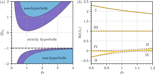
Figure 2: Hyperbolicity of the morphodynamic model equations depends on the bed load function $Q$. (a) Regions of non-hyperbolicity as a function of Fr and $Q_{h_{0}}$, for fixed $Q_{u_{0}}=0.1$ (purple shading), $1$ (blue shading) and $Q_{\psi_{0}}=0$. Outside these regions, the model is strictly hyperbolic, save along the bounding curves $G_{\pm}$ (dotted lines) and the special case $Q_{h_{0}}=-1$ (dashed line), where one of the roots of $c$ intersects with the solid mass transport characteristic. (b) System characteristics as a function of Fr for $Q_{u_{0}}=0.1$, $Q_{\psi_{0}}=0$ and $Q_{h_{0}}=0.095$ (dotted lines), $0.105$ (solid lines). We label the curves I–IV according to the ordering of the corresponding characteristics derived in (21) for the $Q=0$ case.

The axes have been chosen so as to encompass very general $Q$ closures. However, fortunately in applications sediment flux typically depends only very weakly, if at all on the flow depth, so $|Q_{h_{0}}|\ll 1$ is expected. In fact, it is common in fluvial models to have $Q_{u_{0}}$ strictly positive and $Q_{h_{0}}=0$ or $-1\ll Q_{h_{0}}<0$ (in the latter case, if a Manning friction law is employed). Therefore, most studies that include bed load operate in a regime where (48) is satisfied.

This analysis suggests an alternative to the regularisation strategy of §3.3, since adding even a small bed load flux term can ensure that the model equations are well posed, provided that (48) is satisfied. We visualise the effect of bed load on the system characteristics in figure 2(b), either side of the threshold $Q_{h_{0}}=Q_{u_{0}}$ where the system loses hyperbolicity. We plot $\Real(\lambda_{1})$ as a function of Fr for $Q_{u_{0}}=0.1$ and $Q_{h_{0}}=0.095$ (dotted lines), $0.105$ (solid lines). The four branches of $\lambda_{1}$ are labelled I–IV, according to the ordering of the corresponding modes in the $Q=0$ case, adopted in §3.2.2. When $Q_{h_{0}}=Q_{u_{0}}=0.1$ (not shown), the mode II and IV characteristics intersect at a single point, $\mbox{{Fr}}=\sqrt{1.1}\approx 1.05$ in this case, which is easily calculated using the expressions in (47). Decreasing $Q_{u_{0}}$ (so that $Q_{u_{0}}<Q_{h_{0}}$) causes these characteristics to coalesce into a complex conjugate pair, resulting in a region ($0.95\lesssim\mbox{{Fr}}\lesssim 1.15$) where the system is non-hyperbolic. Conversely, increasing $Q_{u_{0}}$ separates the intersecting characteristics so that four real values are present across all Froude numbers. (Note that these separated curves are labelled with both II and IV, since they originate from different modes at either end.) The other two characteristics (I and III) are essentially unaffected by small changes in the bed load.

4 Implications

In this section, we examine the above analyses in greater detail by choosing some closures for the morphodynamic model equations (6a–d). We focus initially on the primary case of the basic suspended load model, before investigating the effects of incorporating eddy viscosity and bed load. It is our contention that the specifics of individual modelling terms should not qualitatively affect the observations below, provided that they are consistent with the essential physics of the problem. Therefore, in this exposition, we favour simple phenomenological formulae.

4.1 Model closures

In order to capture a range of different sedimentary flows, from dilute suspensions to fully granular flow, we use a mixed drag formulation that depends on the bulk solid fraction, writing

$$\tilde{\tau}=(1-\psi)\tilde{\tau}_{f}+\psi\tilde{\tau}_{g},$$ (49)

where $\tilde{\tau}_{f}$ and $\tilde{\tau}_{g}$ are fluid and granular drag laws respectively. We assume that the bed is a saturated mixture of fluid and sediment containing the maximum possible sediment concentration $\tilde{\psi}_{b}=\tilde{\psi}^{*}$. The maximum solid fraction $\tilde{\psi}^{*}$ depends on how efficiently particles can be packed and is typically observed to be around $60$–$70\%$ (Santiso & Müller, 2002; Farr & Groot, 2009). Since $\psi=\tilde{\psi}/\tilde{\psi}_{b}$, we have $0\leq\psi\leq 1$ for all flows and therefore (49) contains all weighted combinations of fluid and granular drag. For the fluid law, we employ the common Chézy formula for turbulent shear stress, $\tilde{\tau}_{f}=C_{d}\tilde{\rho}\tilde{u}^{2}$, where $C_{d}$ is a drag coefficient, which we assume to be constant. For the granular drag, we use the frictional law due to Pouliquen & Forterre (2002), which sets $\tilde{\tau}_{g}=\mu(I)\tilde{\rho}g\cos(\phi)\tilde{h}$. The phenomenological parameter $\mu$ is modelled as an increasing function of the dimensionless inertial number $I\equiv uh^{-3/2}d\mbox{{Fr}}$, where $d=\tilde{d}/\tilde{h}_{0}$ and $\tilde{d}$ denotes the characteristic diameter of the sediment particles. It is constructed so as to vary smoothly between a lower (static) limit $\mu_{1}$ and an upper (dynamic) bound $\mu_{2}$, with $0<\mu_{1}<\mu_{2}$, and takes the form

$$\mu(I)=\mu_{1}+\frac{\mu_{2}-\mu_{1}}{1+\beta I^{-1}},$$ (50)

where $\beta$ is a positive constant that may be determined experimentally.

We suppose that mass transfer is governed by the competing processes of bed erosion at a rate $\tilde{E}$ and particle deposition at rate $\tilde{D}$, writing $\tilde{\Gamma}=\tilde{E}-\tilde{D}$. Since these processes take place at the scale of individual particles, we opt to non-dimensionalise these closure terms using the velocity $\tilde{u}_{p}=(g^{\prime}_{\perp}\tilde{d})^{1/2}$, where $g_{\perp}^{\prime}=g\cos\phi\left(\tilde{\rho}_{s}/\tilde{\rho}_{f}-1\right)$ is the reduced gravity for a particle in dilute suspension, resolved perpendicular to the slope. The dimensionless transfer rates are then $E_{p}=\tilde{E}/\tilde{u}_{p}$ and $D_{p}=\tilde{D}/\tilde{u}_{p}$. This rescaling allows us to fix appropriate dimensionless constants for these closures when considering the steady balance $E_{p}=D_{p}$ independently. However, note that care must be taken when reintroducing these terms into (6a–d), which uses a different velocity scale for $\partial b/\partial t$. Specifically, if $\Gamma_{p}\equiv E_{p}-D_{p}$, then (5h) implies that $\Gamma=\Gamma_{p}\mbox{{Fr}}d^{1/2}(\rho_{s}/\rho_{f}-1)^{1/2}\cot\phi$.

Entrainment of particles into the flow is caused by turbulent shear stresses at the bed, which must overcome the static friction experienced by resting grains. Competition between $\sim\tilde{\tau}\tilde{d}^{2}$ drag forces and $\sim\tilde{\rho}_{f}g_{\perp}^{\prime}\tilde{d}^{3}$ frictional forces (assumed proportional to the submerged weight of individual grains) can be captured by their ratio, the dimensionless Shields number $\theta\equiv\tilde{\tau}/(\tilde{\rho}_{f}g_{\perp}^{\prime}\tilde{d})$. Experimental observations for dilute flows suggest that at sufficiently high drag, flow erosion obeys a power law of the form $\tilde{E}\propto(\theta-\theta_{c})^{3/2}$, where $\theta_{c}$ is a critical Shields number below which there is no entrainment. Beyond this there is considerable disagreement concerning both the exact functional form for $\tilde{E}$ and its magnitude (Lajeunesse et al., 2010). Moreover, it is unclear whether this general erosion model applies for more concentrated suspensions, where effects such as the pore water pressure modify the force relationship encapsulated in the Shields number. Since our aim here is only to elucidate some general properties of solutions, we prefer simplicity here and suppose that $\tilde{E}$ depends linearly on $\tilde{u}_{p}(\theta-\theta_{c})^{3/2}$. However, we shall make one important modification to this dilute erosion law. Since concentrated layers may be held static on shallow grades by their granular friction, we must not permit erosion to occur in situations where $\theta>\theta_{c}$, yet $\tilde{u}=0$. Therefore, we set $\theta_{c}=\theta_{c}^{*}+\theta_{0}$, where $\theta_{c}^{*}$ denotes the usual critical Shields number (for dilute suspensions) and $\theta_{0}(\tilde{h},\tilde{\psi})=\theta|_{\tilde{u}=0}$, i.e. the Shields number of a resting flow, which may become large as $\tilde{\psi}$ increases. For simplicity, we consider $\theta_{c}^{*}$ constant in this study, even though in principle it depends on flow properties such as the particle Reynolds number $\Rey_{p}\equiv\tilde{u}_{p}\tilde{d}/\tilde{\nu}_{f}$, where $\tilde{\nu}_{f}$ is the kinematic viscosity of the fluid (Soulsby, 1997). On dividing through by $\tilde{u}_{p}$, the dimensionless entrainment rate is then

$$E_{p}(h,u,\psi)=\begin{cases}\varepsilon\left[\theta(h,u,\psi)-\theta_{c}(h,\psi)\right]^{3/2}&\text{if }\theta>\theta_{c},\\ 0&\text{otherwise},\end{cases}$$ (51)

where $\varepsilon$ is a proportionality coefficient that characterises the erodibility of the bed.

We treat sediment deposition as being governed by a process of hindered settling. At low concentrations, particles settle independently, so the (monodisperse) sediment deposits at a rate $\sim\tilde{w}_{s}\psi$, where $\tilde{w}_{s}$ denotes the characteristic falling speed of the grains. As concentrations increase, pure settling becomes disrupted as particles increasingly interact, ultimately shutting off as $\psi\to 1$ and grains can no longer fall (in a time-averaged sense) under gravity. Therefore, we take the deposition term to be

$$D_{p}(\psi)=w_{s}\psi(1-\psi),$$ (52)

where $w_{s}=\tilde{w}_{s}/\tilde{u}_{p}$. This a slight simplification of the widely used formula due to Richardson & Zaki (1954). More detailed and accurate expressions for $D_{p}$ typically involve empirical fits featuring the same essential form (e.g. Spearman & Manning, 2017).

When considering a bed load, we use the following standard expression, which mirrors the entrainment rate of (51):

$$Q_{p}=\begin{cases}\gamma\left[\theta(h,u,\psi)-\theta_{c}(h,\psi)\right]^{3/2}&\text{if }\theta>\theta_{c},\\ 0&\text{otherwise},\end{cases}$$ (53)

where $Q_{p}$ is a particle-scale non-dimensionalisation such that $Q_{p}=\tilde{Q}/(\tilde{d}\tilde{u}_{p})$ and $\gamma$ is a constant that dictates the flux strength. For example, $\gamma=8$ sets the well-known Meyer-Peter & Müller formula (Meyer-Peter & Müller, 1948). The corresponding flow-scale non-dimensionalisation, as used in (6d) and given by (5i), is $Q=Q_{p}\tilde{d}\tilde{u}_{p}/(\tilde{h}_{0}\tilde{u}_{0})=Q_{p}d^{3/2}(\rho_{s}/\rho_{f}-1)^{1/2}/\mbox{{Fr}}$.

Finally, the basal velocity closure dictates the characteristic downslope flow speed at the bed, during particle entrainment. Where needed, we assume that it can be modelled by a turbulent friction velocity of the form

$$\tilde{u}_{b}=\sqrt{\tilde{\tau}/\tilde{\rho}}.$$ (54)

A large number of free parameters are involved in specifying these various model closures. Therefore, we choose to fix some illustrative values, as listed in table 1, making it clear whenever we deviate from these defaults.

$\tilde{\rho}_{s}/\tilde{\rho}_{f}$	$\tilde{\psi}_{b}$	$C_{d}$	$d$	$\mu_{1}$	$\mu_{2}$	$\beta$	$\varepsilon$	$\theta_{c}^{*}$	$w_{s}$
$2$	$0.65$	$0.01$	$0.01$	$0.1$	$0.4$	$0.1$	$0.01$	$0.05$	$1$

Table 1: Illustrative model parameters. Except where otherwise stated, all results in §4 assume these values. Definitions for these parameters may be found in equations (2), (3b), (49)–(52) and the accompanying text in each case.

An investigation of other parameter choices indicated that our observations below are qualitatively robust to variations in these values.

4.2 Existence of steady layers

We are now in a position to assess when uniform flowing layers can exist in equilibrium. This is dictated by the steady balances in (4a,b), which we recall enforce that drag balances the downslope component of gravitational forcing and that there is no net material transfer between the flow and the bed. Note that these conditions are independent of whether there is a bed load or not. To begin with, we concentrate on the stress balance and assume that mass transfer with the bulk is negligible ($\Gamma\to 0$), thereby automatically satisfying (4b). Substituting our mixed drag law (49) into (4a), non-dimensionalising and rearranging gives the following condition for existence of a steady layer of solid fraction $\psi_{0}$:

$$\tan\phi-(1-\psi_{0})C_{d}\mbox{{Fr}}^{2}=\psi_{0}\mu(d\mbox{{Fr}}).$$ (55)

In the dilute limit, $\psi_{0}\to 0$, where drag is purely fluid-like, this equation selects a unique Froude number, $\mbox{{Fr}}=\sqrt{\tan\phi/C_{d}}$. Such states become unstable when $\mbox{{Fr}}>2$ (Jeffreys, 1925). Conversely, in the concentrated limit, $\psi_{0}\to 1$, where drag is purely granular, steady layers adopt a unique inertial number, given by $I_{0}\equiv d\mbox{{Fr}}=\mu^{-1}(\tan\phi)$. Since $\mu_{1}<\mu(I)<\mu_{2}$, only a range of slope angles (between $\arctan\mu_{1}$ and $\arctan\mu_{2}$) are permitted. The threshold for linear instability in this case does not depend on $\mu$ and was computed by Forterre & Pouliquen (2003) to be $\mbox{{Fr}}>2/3$.

For intermediate values of $\psi_{0}$, since the left-hand hand side in (55) is a decreasing function of Fr and unbounded below, the steady drag balance may be satisfied as long as $\tan\phi\geq\psi_{0}\mu_{1}$. The effect of the Chézy drag term thereby relaxes the limits on existence imposed by the granular law. Steady layers that are more dilute can exist in mobile equilibrium at shallower slope angles, i.e. down to $\arctan(\psi_{0}\mu_{1})$, while steep steady flows ($\tan\phi\to\infty$) may always be maintained at a suitably high Fr, since the turbulent drag, $C_{d}\mbox{{Fr}}^{2}$, is not bounded above. However, note that such solutions are not necessarily stable. Indeed, the stability threshold for these flows may be readily computed using Trowbridge’s criterion (13). After non-dimensionalising (49) and differentiating, one sees that $\tau_{u_{0}}=[2(1-\psi_{0})C_{d}\mbox{{Fr}}^{2}+\psi_{0}\mu^{\prime}I_{u_{0}}]\cot\phi$, where $\mu^{\prime}=\partial\mu/\partial I|_{I=I_{0}}$ and $I_{u_{0}}=\partial I/\partial u|_{h,u=1}=d\mbox{{Fr}}$. Likewise, $\tau_{h_{0}}=\psi_{0}[\mu(d\mbox{{Fr}})+\mu^{\prime}(d\mbox{{Fr}})I_{h_{0}}]\cot\phi$, with $I_{h_{0}}=\partial I/\partial h|_{h,u=1}=-\frac{3}{2}d\mbox{{Fr}}$. On substituting these expressions into (13) and rearranging, one sees that these states are unstable when

$$(1-\psi_{0})C_{d}(\mbox{{Fr}}-2)+\psi_{0}d\mu^{\prime}(3/2-1/\mbox{{Fr}})>0.$$ (56)

Note that this criterion smoothly interpolates between the $\mbox{{Fr}}=2$ and $\mbox{{Fr}}=2/3$ thresholds for the special cases of purely fluid ($\psi_{0}=0$) and granular ($\psi_{0}=1$) flows.

We summarise the existence of non-erosive layers subject to the drag law (49) in figure 3.

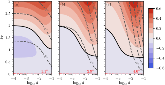
Figure 3: Existence of steady layers for our mixed drag formulation (49), without morphodynamics. Dashed lines show the existence of steady flows at fixed slope angles as labelled, with the lowest red dashed line indicating the minimum slope angle $\phi=\arctan(\psi_{0}\mu_{1})$. Filled contours show maximum values of the non-dimensional linear growth rates given in (11). Stable (blue) and unstable (red) regions are separated by the neutral stability boundary (56) plotted in solid black. Successive panes represent increasing solid fractions $\psi_{0}$ from left to right as follows: ($a$) 0.2, ($b$) 0.5 and ($c$) 0.8.

Dashed contours trace out the unidimensional family of steady layers for each slope angle, across $(d,\mbox{{Fr}})$-parameter space, computed from (55), with the three panes corresponding to different fixed solid fractions, $\psi_{0}=0.2$, $0.5$ and $0.8$, from left to right. The minimum slope angles for steady flows (dashed red contours) follow the line $\mbox{{Fr}}=0$. Red and blue filled contours show the asymptotic growing and decaying growth rates of perturbations respectively, computed by substituting $\tau_{u_{0}}$ and $\tau_{h_{0}}$ from above into the limiting formula given earlier in (12). These are separated by the neutral stability boundary (56), which is displayed in solid black. When $d\ll 1$ (small particles, relative to the flow depth), the drag is dominated by the Chézy term. In this regime, which covers most physically realisable grain sizes, growth rates are essentially independent of $d$ and the stability boundary is $\mbox{{Fr}}\approx 2$. Increasing $d$ outside this region leads to less stable flows and lowers the stability boundary. Increasing the solid fraction generally leads to less severe growth rates, but decreases the range of slope angles that permit stable steady flows (through increasing the minimum slope angle). We find the qualitative properties of this plot to be largely insensitive to our specific choices of $C_{d}$, $\mu_{1}$, $\mu_{2}$ and $\beta$ whose values were given in table 1.

When morphodynamics is non-negligible, steady flows must also satisfy (4b). That is, erosion and deposition must be everywhere in balance, $E_{p}(h,u,\psi)=D_{p}(\psi)$. This condition dictates the solid fractions where mass transfer can be in equilibrium. Despite our efforts to obtain simple closures in (51) and (52), it is a complex nonlinear equation that depends on many physical parameters. Nevertheless, we can determine some generic properties of solutions.

We first consider the system parameters to be fixed (but arbitrary) and suppose that the flow is in uniform steady balance with its drag (so $h=u=1$), leaving $D_{p}$ and $E_{p}$ functions of $\psi$ only. We also assume that $\theta>\theta_{c}$, so that there is some particle entrainment. Then, in particular, $E_{p}(0)>0$ and $E_{p}(1)>0$. Conversely, the deposition rate curve (52) always obeys $D_{p}(0)=D_{p}(1)=0$. Therefore, since $E_{p}-D_{p}>0$ for both $\psi=0$ and $1$, either: (a) there exist an even number of coexistent steady flows with different solid fractions, (b) erosion balances deposition exactly at a turning point in $E_{p}-D_{p}$ or (c) erosion always exceeds deposition. We visualise these three cases in figure 4, where we plot $D_{p}(\psi)$ and $E_{p}(\psi)$ at different values of Fr, using the illustrative model parameters of table 1.

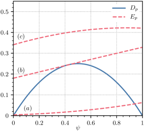
Figure 4: Example deposition and erosion closures, as functions of the solid fraction $\psi$. Steady flows occur where $D_{p}$ and $E_{p}$ intersect. There are three cases: ($a$) two steady states, one dilute and one concentrated ($\mbox{{Fr}}=0.75$); ($b$) a single steady state where $E_{p}$ is tangent to $D_{p}$ ($\mbox{{Fr}}\approx 2.63$); ($c$) erosion always exceeds deposition (no steady states) ($\mbox{{Fr}}=3.25$).

Aside from where explicitly stated otherwise, these parameters are fixed for the remainder of this section. Note that our choice of $D_{p}$ does not depend on Fr, while the Froude number dependence of $E_{p}$ enters through the basal drag term in the Shields number.

Case ($a$), where there are multiple steady flows, occurs at lower Fr numbers. Here, erosion increases with solids concentration, intersecting the deposition curve at two points. This leads to two corresponding steady flows: one dilute and one relatively concentrated. Additional intersections (leading to three or more steady flows) are a possibility, but would require a very particular erosion curve. Physical intuition suggests that the dilute solution is stable, since perturbations in either direction cause negative feedback: decreasing $\psi$ away from this state leads to $E_{p}>D_{p}$, while increasing $\psi$ leads to $E_{p}<D_{p}$. Likewise, the concentrated solution (at $\psi\approx 0.94$ in figure 4) invites either runaway deposition (if $\psi$ decreases) or runaway erosion (if $\psi$ increases). This process suggests a possible mechanism underlying sediment distribution in debris flows, which commonly feature an unsteady highly concentrated front trailed by a steady dilute layer (Pierson, 1986; Hungr, 2000; Ancey, 2001). As Fr increases in figure 4, the pair of steady flows coalesces at a single point; this is case ($b$). Beyond this point, no steady solutions exist, case ($c$). Here, erosion everywhere exceeds deposition. Uniform layers in this case can never be truly steady, since they can only satisfy one of (4a,b). If the drag is ever in equilibrium with gravitational forces, then net entrainment injects material into the flow.

4.3 Global morphodynamic modes

The instability mechanism identified in figure 4 is purely morphodynamic and depends on a straightforward criterion: states are unstable to this mode if $\Gamma_{\psi_{0}}>0$. The process is fundamentally an instability to uniform perturbations in flow concentration, though since there is no intrinsic dependence upon spatial gradients we might anticipate that it manifests as a destabilising feature at all wavenumbers. However, this picture is a simplification, since it omits feedbacks from the other flow fields. The full situation for uniform disturbances is contained within our analysis of zero-wavenumber perturbations in §3.2.1, where we computed the general growth rates of the four different linear stability modes for $k=0$, two of which are always neutrally stable. As discussed earlier, if the approximation of small $\Gamma_{u_{0}}$ can be made, the two remaining modes may be understood simply: one is inherited from the hydrodynamic stability problem, the other contains morphodynamic feedbacks. Their growth rates are given in (18a,b). The morphodynamic rate in  (18b) may by understood as a competition between two mechanisms for growth in $h$ and $\psi$. The process for $\psi$ (when $\Gamma_{\psi_{0}}>0$) has already been outlined. If $\Gamma_{h_{0}}>0$, then a small increase in the steady layer height leads to net entrainment which, via (6a), enhances growth in $h$ in turn. Likewise, a small decrease in $h$ would cause the depth to decrease away from its steady value. Conversely, if $\Gamma_{h_{0}}<0$, then this term is stabilising. If $\Gamma_{h_{0}}$ is negligible with respect to $\Gamma_{\psi_{0}}(1-\psi_{0})$, then the morphodynamic mode has approximate growth rate $\sigma^{*}_{m}$, defined by

$$\sigma_{m}^{*}=\Gamma_{\psi_{0}}(1-\psi_{0}).$$ (57)

In this case, stability is only governed by the mechanism for concentration growth encapsulated by figure 4.

The accuracy of the above physical picture depends on the reliability of the approximations made in reaching (18a,b) and (57). These estimates are plausible (especially at lower $\psi_{0}$), since we might expect the relative steepness of the hindered settling curve (plotted in figure 4) to be more significant than gradients in $E_{p}$, which are solely responsible for dictating $\Gamma_{h_{0}}$, $\Gamma_{u_{0}}$ and depend on the small parameters $\varepsilon$ and $C_{d}$.

For a more detailed analysis, in figures 5(a) and (b) we show both non-zero branches of the exact growth rates $\sigma$ (solid lines) for global disturbances (which are purely real), as given in (16a)–(17b), for (a) dilute and (b) concentrated states.

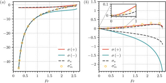
Figure 5: Growth rates for uniform ($k=0$) perturbations as a function of Fr, for the (a) dilute and (b) concentrated steady solution families identified in figure 4. Solid curves show the two non-zero branches of the exact growth rate $\sigma$, computed from the formulae in (16b)–(17b). The signs given in the legend indicate the branch, according to the sign of $\pm\sqrt{s_{c}}$ in (16b). Also plotted are two approximations to the exact rates, $\sigma_{a}$ (dashed lines), as defined in (18), and $\sigma_{m}^{*}$ (yellow circles), as defined in (57).

On the same axes, we plot both approximations to the rates: the more general formulae from (18a,b), which we denote $\sigma_{a}$ (dashed lines), and the cruder approximation to the morphodynamic mode rate $\sigma_{m}^{*}$ (yellow circles), made above in (57). For the dilute states, we confirm that $\sigma<0$ across the range where steady layers exist ($0.22\lesssim\mbox{{Fr}}\lesssim 2.62$). Moreover, both branches of $\sigma$ are well approximated by $\sigma_{a}$ for $\mbox{{Fr}}\lesssim 1.5$, and $\sigma_{m}^{*}$ lies very close to its corresponding branch of $\sigma_{a}$, indicating that $\Gamma_{\psi_{0}}$ is indeed primarily responsible for setting the sign of $\sigma$ in this case. At higher Fr, the approximating curves are less accurate. However, this is to be expected. Whereas at low Fr, the dilute solutions have $\psi_{0}\approx 0$, which is where the hindered settling curve is at its steepest (and consequently where $|\Gamma_{\psi_{0}}|$ can be considered large compared with other derivatives of $\Gamma$), for higher Fr states have higher $\psi_{0}$ and the approximations of negligible $|\Gamma_{h_{0}}|$ and $|\Gamma_{u_{0}}|$ gradually break down as $\psi_{0}$ approaches the turning point in $D_{p}$ (see figure 4). However, we note that throughout, $\sigma_{m}^{*}$ lies close to $\sigma_{a}$ since $|\Gamma_{h_{0}}|$ is small for dilute states. Furthermore, we need only be strictly concerned with $\mbox{{Fr}}\lesssim 1$, since outside this regime layers are susceptible to high wavenumber instabilities.

By contrast, the approximations to the growth rates for the concentrated solutions, in figure 5(b), are not especially good, as highlighted by the figure insert. Therefore, $\Gamma_{u_{0}}$ cannot be neglected here. Unfortunately, while perturbations in $h$ and $\psi$ and their respective feedbacks may be understood in simple physical terms, this is not easy to do in general for $u$, due to the many interacting contributions to momentum present in the governing equations. However, in this particular case, we note that the intuition that concentrated steady states are typically unstable is borne out, meaning that the feedbacks omitted in making the approximation $\sigma_{a}$ are not stabilising on aggregate. In fact, this is guaranteed, since the pair of steady states in figure 4 arises in a saddle-node bifurcation as Fr is decreased from infinity. This implies that, since the dilute flow is stable, the concentrated flow must have at least one unstable direction.

4.4 Linear growth rates for general wavenumbers

Instability to uniform disturbances is not the only feature introduced by the presence of morphodynamics, as our earlier analysis in §3.2 indicates, since states are also vulnerable to the high-wavenumber instability near unit Froude number. Therefore, we broaden the discussion to incorporate the full linear stability problem. We begin by numerically solving the eigenproblem in (8) using our chosen model closures, over a range of finite wavenumbers. Each of the four eigenmodes in the problem possesses a linear growth rate continuously parametrised by $k$. As in §3.2.2, we label the modes I–IV according to the ordering of their asymptotes used in (25a–d). Recall that in the high-$k$ regime, modes I & II are analogues to the modes of the purely hydraulic stability problem, whereas III & IV are additional morphodynamic modes that, involve perturbations in the solid fraction and bed surface respectively.

We denote the growth rates of each mode, indexed by wavenumber as $\sigma_{n}(k)$ for $n=1,\ldots,4$. In figure 6(a) we plot $\max_{n}\Real(\sigma_{n})$ versus $k$, for states on the dilute solution branch.

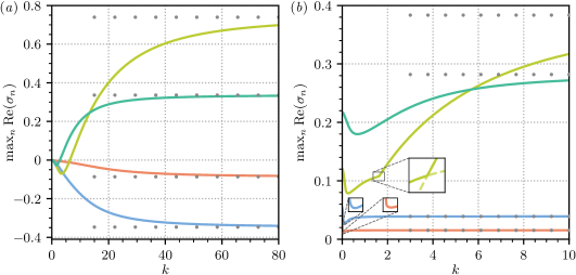
Figure 6: Perturbation growth rates for morphodynamic states as functions of wavenumber in the unregularised problem ($\nu=0$). The curves were computed by taking the maximum real part of the four normal mode growth rates arising from (8), across a range of wavenumbers $k$, for states on the (a) dilute and (b) concentrated solution branches identified in figure 4. The Froude numbers are $\mbox{{Fr}}=0.5$ (orange), $0.75$ (blue), $1.25$ (olive), $2$ (teal). High-$k$ asymptotes, computed from maxima of the four expressions (25a–d), are plotted in dotted grey.

Additionally, we plot their limiting high-$k$ growth rates, taken from the maxima of the four expressions derived in (25a–d), in dotted grey. Each curve passes through the origin, since the maximum growth at $k=0$ is given by the neutral modes for these states. The $\mbox{{Fr}}=0.5$ and $0.75$ solutions are stable to all perturbations, just as they would be in the non-erosive case, with the latter solution being more strongly damped. The $\mbox{{Fr}}=1.25$ curve is stable to long-wavelength disturbances and becomes unstable at $k\approx 6$. Its maximum over all $k$ is given by its asymptotic value, to which it converges more slowly than the other curves. This solution would be stable in the non-erosive case: given the same solid fraction ($\psi_{0}\approx 0.02$), according to (56), non-erosive states turn unstable at $\mbox{{Fr}}\approx 1.98$. The $\mbox{{Fr}}=2$ state is stable for a narrower range of wavelengths, becoming unstable at $k\approx 3$. This state (which has $\psi_{0}\approx 0.1$) would also be unstable in the non-erosive situation. Its asymptotic growth rate is lower than the $\mbox{{Fr}}=1.25$ curve, which we shall see shortly is because it lies further from the $\mbox{{Fr}}=1$ singularities present in (25b,d). Aside from a narrow interval ($k\lesssim 1.5$) at small $k$ in the $\mbox{{Fr}}=2$ case where mode I dominates (not visible at this scale), each of these maximum growth rates for dilute states are everywhere given by the growth of the morphodynamic mode IV.

In figure 6(b), we plot the corresponding maximum growth rate curves for the concentrated solution branch. These match the intuition from §4.3, that concentrated states should be everywhere unstable (since we expect the basic global instability mechanism to persist regardless of $k$). Growth at $k=0$ is a local maximum for each Fr and the corresponding instability is due to mode III, which dominates over all $k$ for $\mbox{{Fr}}=0.5$, $0.75$ and $\mbox{{Fr}}=2$. (The two lower Fr growth rate curves turn sharply at $k\approx 0.025$ and $0.075$ respectively, but are nevertheless smooth, as indicated on the insert.) Conversely, the $\mbox{{Fr}}=1.25$ curve is formed by a crossing of growth rates for modes III and IV, the latter of which is neutral at $k=0$. The crossing point (at $k\approx 1.6$) is shown in an insert, with the subdominant portions of the mode III and IV curves also included (dashed lines).

The variations of the modes as functions of Froude number are encapsulated in figure 7.

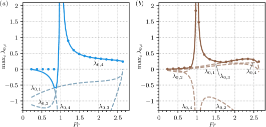
Figure 7: The maximum of the high-wavenumber asymptotic growth rates, $\max_{i}\lambda_{0,i}$, plotted with solid curves as a function of Fr, for the (a) dilute and (b) concentrated solution branches. With dashed lines we plot the individual $\lambda_{0,i}(\mbox{{Fr}})$ curves, as labelled for $i=1,\ldots,4$. Also plotted (filled circles) are the maximum growth rates of the corresponding solutions, over all wavenumbers, i.e. $\max_{k,n}\Real[\sigma_{n}(k)]$.

Here, we plot the asymptotic ($k\gg 1$) growth rates $\lambda_{0,i}$, given in (25a–d), for $i=1,\ldots 4$, with dashed lines. Their maximum for each Fr is overlaid as a solid line. With filled circles, we plot the maximum growth rate over all $k$. Therefore, any discrepancy between the solid lines and circles indicates that maximal growth is attained at some finite wavenumber. Figure 7(a) presents the data for the dilute solutions. At low Fr, solutions are stable and the maximum possible growth is zero, due to the ($k=0$) neutral modes. The asymptotic growth rate is dictated by the mode IV curve, which is briefly surpassed by mode I at $\mbox{{Fr}}\approx 0.85$, before growth is dominated by the singular behaviour of modes II (for $\mbox{{Fr}}<1$) and IV (for $\mbox{{Fr}}>1$), which diverge at $\mbox{{Fr}}=1$ with opposite sign. This induces instability at $\mbox{{Fr}}\approx 0.9$. For all higher Froude numbers, the solutions remain unstable, even though they would be sufficiently dilute to remain stable well past $\mbox{{Fr}}=1$ if morphodynamic effects were neglected. We also note that the asymptotic rate correctly identifies the onset of instability and matches the maximum rate thereafter, thereby justifying the focus on short wavelengths in our analysis.

The corresponding curves for the concentrated solution branch are shown in figure 7(b). As expected, this also features a singularity at $\mbox{{Fr}}=1$ and is everywhere unstable. The maximum growth rates (filled circles) exactly match the corresponding asymptotic limits, except at low Froude number ($\mbox{{Fr}}\lesssim 0.85$), where growth at $k=0$ is slightly larger than in the $k\gg 1$ regime, as we saw in figure 6(b). Mode III is always unstable and dominates the other modes over a large region. Near the singularity it is surpassed by modes II (for $\mbox{{Fr}}<1$) and IV (for $\mbox{{Fr}}>1$) and it is briefly surpassed again by mode IV near $\mbox{{Fr}}\gtrsim 2.6$, where the dilute and concentrated solution branches coalesce.

4.5 Effect of bed erodibility

In addition to the singularity introduced at unit Froude number, a further effect of the morphodynamics on dilute states may by identified in figure 7(a). In the limit of weak sediment entrainment, $\varepsilon\to 0$, mode I must turn unstable at $\mbox{{Fr}}=2$, due to the classical roll wave instability for Chézy bottom drag (Jeffreys, 1925). Conversely, in the regime of figure 7 ($\varepsilon=0.01$), this mode remains stable throughout the range of Fr where steady states exist ($0.22\lesssim\mbox{{Fr}}\lesssim 2.62$). Unstable growth only occurs for mode IV.

We observe the effect of increasing $\varepsilon$ from a weakly erodible regime by reproducing the figure 7(a) plot for dilute states at various values of $\varepsilon$, in figure 8.

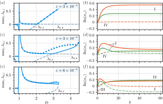
Figure 8: Effect of the bed erodibility $\varepsilon$ on the growth rates of the unstable modes, showing the suppression of mode I (associated with roll wave instability) as $\varepsilon$ increases. The left-hand plots (a,c,e) show maximum asymptotic growth rates ($\max_{i}\lambda_{0,i}$) as a function of Fr for dilute states (solid blue) and individual $\lambda_{0,i}(\mbox{{Fr}})$ curves (grey dashed), as labelled. Maximum growth rates over all wave numbers are plotted with blue circles (as in figure 7, which shows the $\varepsilon=0.01$ case). The right-hand plots (b,d,f) show the growth rates $\sigma_{n}(k)$ of individual modes in dashed lines, as labelled, for $\mbox{{Fr}}=2.6$ (green) and $\mbox{{Fr}}=3.2$ (orange). The maxima of these curves are overlaid as solid lines. The erodibility values for each row are (a,b) $\varepsilon=3\times 10^{-4}$, (c,d) $\varepsilon=3\times 10^{-3}$ and (e,f) $\varepsilon=6\times 10^{-3}$.

The other model parameters remain as stated in table 1. Beginning with the case of small $\varepsilon=3\times 10^{-4}$, in figure 8(a), the signature of hydraulic roll wave instability is clear. Mode I becomes unstable at a Froude number just above $2$ and immediately dominates over the morphodynamic mode. Outside the singular point $\mbox{{Fr}}=1$, the high-$k$ growth rate of the latter mode (IV) is $O(\varepsilon)$, which may be confirmed by consulting the formula derived in (25d) and the closure for entrainment in (51). Consequently, there is a narrowing of the effective influence of the singularity, relative to the picture in figure 7(a), and away from this region, mode IV is only very weakly unstable. In figure 8(b), we plot $\Real(\sigma_{n})$ as a function of $k$ for modes I & IV at $\mbox{{Fr}}=2.6$ (green) and $3.2$ (orange). Both curves for mode I are close to the corresponding unstable growth rates in the limiting case $\varepsilon\to 0$ with purely Chézy drag, which asymptote to exactly $0.3$ and $0.6$ respectively, by equation (12).

We increase $\varepsilon$ by an order of magnitude in figures 8(c–f). When $\varepsilon=3\times 10^{-3}$, growth in the $1<\mbox{{Fr}}\lesssim 2.3$ range is now dominated by the morphodynamic mode and $\lambda_{0,1}$ has substantially decreased, remaining negative until $\mbox{{Fr}}\approx 2.56$. However, $\Real(\sigma_{1})$ no longer attains its maximum in the high-$k$ limit. Indeed, when $\mbox{{Fr}}\gtrsim 2.3$, the most significant growth comes from mode I at finite $k$, as evidenced by figure 8(c). By comparing the $\Real(\sigma_{1})$ curves in figure 8(d) with their counterparts in figure 8(b) we see that growth of mode I is suppressed in the short-wavelength regime as $\varepsilon$ increases. On proceeding to $\varepsilon=6\times 10^{-3}$, these trends continue. The plots in figures 8(e,f) show that growth of the morphodynamic mode dominates over the range $1<\mbox{{Fr}}\lesssim 2.8$, before being surpassed by mode I growth at low $k$. Interestingly, mode I is now only unstable across a limited band of wavelengths. Numerical inspection at indicates that at finite $k$, away from their asymptotic limiting expressions in (22), each eigenmode contains components of all the flow variables $h$, $u$, $\psi$ and $b$. Therefore, at high enough $\varepsilon$, there are no ‘purely hydraulic’ instabilities, including classical roll waves. However, this does not prohibit the existence of roll waves that are intrinsically coupled with the bed and concentration dynamics.

Due to the complexity of the analytic expression for $\lambda_{0,1}$, given in (25a) and (26) it is difficult to appreciate directly why mode I ultimately becomes suppressed when morphodynamic effects are significant. Instead, we can look at a simplified case, where the drag function is purely fluid-like, $\tilde{\tau}=\tilde{\tau}_{f}=C_{d}\tilde{\rho}\tilde{u}^{2}$, and the bottom friction velocity $\tilde{u}_{b}$ is neglected. Then, $\tau_{h_{0}}=\Gamma_{h_{0}}=\upsilon_{0}=0$, $\tau_{u_{0}}=2$ and (25a) simplifies to

$$\lambda_{0,1}=\frac{\mbox{{Fr}}-2}{2}+\frac{\Gamma_{u_{0}}}{4\mbox{{Fr}}(\mbox{{Fr}}+1)}\left[(1-\rho_{b})(\mbox{{Fr}}-1)-2\rho_{b}\mbox{{Fr}}\right].$$ (58)

The first term in this expression stems from the hydraulic limit and yields the correct stability threshold in that case ($\mbox{{Fr}}=2$). Provided that both $\mbox{{Fr}}>1$ and $\rho_{b}>1$ (i.e. the bed density exceeds the bulk density), the second term is strictly negative. Moreover, on referring back to the mass transfer closures (51) and (52), we see that it is proportional to $\varepsilon$. Therefore, greater erodibility decreases $\lambda_{0,1}$ and correspondingly increases the stability threshold for mode I.

In the next two subsections, we investigate the effect of eddy viscosity and bed load on linear growth rates in the morphodynamically dominated regime. We do not independently investigate varying $\varepsilon$ in these cases. However, our numerical observations indicate that, away from $\mbox{{Fr}}=1$, its essential effect is preserved. Namely, that as $\varepsilon$ increases from a negligible value, the $O(\varepsilon)$ bed mode (IV) growth rates become larger and there is a corresponding suppression of mode I.

4.6 Effect of eddy viscosity

Figure 9 demonstrates the effect of the eddy viscosity term studied in §3.3.

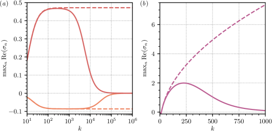
Figure 9: Effect of the eddy viscosity regularisation term on maximum growth rates. Curves for the dilute solution branch are shown with $\nu=0$ (dashed) and $10^{-4}$ (solid). The Froude numbers are: (a) $\mbox{{Fr}}=0.5$ (orange) and $1.5$ (red); (b) $\mbox{{Fr}}=1$ (purple).

The size of the parameter $\nu$ sets the scale over which diffusive effects are important. If chosen sufficiently small, the term only influences the high-$k$ regime. In figure 9(a), we plot maximum normal mode growth rates for dilute solutions with $\mbox{{Fr}}=0.5,1.5$, $\varepsilon=0.01$, $\nu=10^{-4}$ (solid lines) and compare these with the corresponding rates for the unregularised system, $\nu=0$ (dashed lines). At low $k$ (including $0\leq k<10$, not shown), the growth rates are essentially unchanged by the presence of the dissipative term. Then, at higher $k$, both rates for the regularised problem converge to exactly zero, where they remain in the high-$k$ limit. These may be compared with the analytical formulae in (43a–c). Computing them for our particular parameters confirms that both cases are dominated by the asymptote $\sigma=0+O(k^{-1})$, corresponding to perturbations of the bed (43b). For the $\mbox{{Fr}}=0.5$ case, the growth rate increases when it approaches this limit at high $k$. However, note that since it approaches zero from below, this does not affect flow stability. Therefore, we conclude that, away from the singularity at $\mbox{{Fr}}=1$, the addition of the diffusive term succeeds in damping out short-wavelength disturbances without affecting the system outside the asymptotic regime. The behaviour at $\mbox{{Fr}}=1$ is shown in figure 9(b) and confirms the successful regularisation of the growth rate singularity. While the unregularised rate diverges like $\sim k^{1/2}$ (as shown in §3.2.2), when $\nu=10^{-4}$ it decays to zero within $0\leq k\lesssim 10^{3}$. It reaches a maximum growth rate of approximately $2$, around 3–6 times the magnitude of unregularised growth rates either side of the singularity at $\mbox{{Fr}}=0.75$ and $1.25$, plotted in figure 6(a).

Figure 10 shows the effect of regularisation on concentrated states.

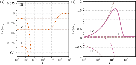
Figure 10: Individual growth rates as a function of $k$ for concentrated steady states. The curves are labelled I–IV according to their corresponding linear stability modes in the $\nu=0$ analysis of §3.2.2. Unregularised rates are plotted with dashed grey lines; regularised rates ($\nu=10^{-4}$) with dotted lines. The maximum over all curves in the $\nu=10^{-4}$ case is overlaid as a solid line. The Froude numbers are (a) 0.5 and (b) 1.

In these plots we include additional detail, plotting the growth rates for all four modes. Dashed lines show curves with $\nu=0$; dotted lines show the corresponding rates with $\nu=10^{-4}$. We label these I–IV by numerically computing the asymptotic rates (25a–d) and (30) for the unregularised system, which match the corresponding regularised rates at lower $k$. The case of $\mbox{{Fr}}=0.5$, away from the singularity is given in figure 10(a). Both hydrodynamic modes (I and II) are severely damped at high $k$. On checking these curves against the asymptotic rates in (43a–c), we find that mode I corresponds to (43a), scaling as $\sim-k^{2}$ asymptotically, while mode II eventually converges to $\lambda_{-}\approx-4\times 10^{4}=-1/\nu\mbox{{Fr}}^{2}$ in this case (outside the range of the figure axes). The mode IV rate increases as $k$ increases, eventually asymptoting to $0$. Finally, as argued in §3.3, mode III, which asymptotes to $\lambda_{+}$ ($\approx 0.015$), is not much affected by the eddy viscosity term, provided that $\nu$ is small relative to the other terms in (41). The situation at the $\mbox{{Fr}}=1$ singularity for concentrated states is shown in figure 10(b). When $\nu=0$, the mode II and IV growth rates can be seen diverging to $-\infty$ and $+\infty$ respectively as $k\to\infty$. As established in §3.2.2, these scale like $\sim\pm k^{1/2}$, asymptotically – while modes I and III converge to $\lambda_{0,1}$ ($\approx 0.04$) and $\lambda_{0,3}$ ($\approx 0.07$) respectively. With the addition of regularisation, the modes qualitatively mirror the $\mbox{{Fr}}=0.5$ case: the hydraulic modes are strongly damped, while mode IV no longer diverges and decays to zero, being eventually surpassed by mode III which is essentially unaffected by the eddy viscosity.

We have briefly experimented with introducing an additional diffusive term to the solid mass transport equation. This takes the form $\frac{\partial~{}}{\partial x}(\kappa h\frac{\partial\psi}{\partial x})$ and is added to the right-hand side of (6b), thereby contributing an additional non-zero term $D_{23}=\kappa$ to the matrix $\mathsfbi{D}$ in the linear stability eigenproblem (31). The free parameter $\kappa=\tilde{\kappa}/(\tilde{u}_{0}\tilde{l}_{0})$, where $\tilde{\kappa}$ is a (constant) characteristic sediment diffusivity sometimes included in models (e.g. Balmforth & Vakil, 2012; Bohorquez & Ancey, 2015). Its inclusion is consistent with the basic physics of sediment transport. However, the effect on the growth rates is modest, for the values explored ($10^{-3}<\kappa<10^{-5}$), effectively serving only to damp mode III at high wavenumbers. Consequently, figure 9 is unaffected, while the maximum unstable growth in figure 10 ultimately rolls off at high $k$, with the roll-off being more severe for larger values of $\kappa$. Therefore, in the context of simple shallow flow modelling, sediment diffusion, combined with momentum diffusion via eddy viscosity, could serve as an unobtrusive way to prevent instabilities from developing over unphysically short length scales.

We now examine the effect of varying $\nu$. Figure 11 shows the reduction of growth rate at the $\mbox{{Fr}}=1$ singularity as $\nu$ is increased over three orders of magnitude for both the (a) dilute and (b) concentrated solution branches.

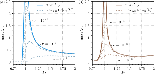
Figure 11: Effect of eddy viscosity size on the severity of morphodynamic instability. Solid curves show the maximum asymptotic growth rates for the unregularised system (as shown previously in figure 7), near the $\mbox{{Fr}}=1$ singularity, for (a) dilute and (b) concentrated steady states. Dotted curves show the maximum growth rates over all wavenumbers and all four modes, for various $\nu$, as labelled.

At $\nu=10^{-4}$, the maximum growth is curtailed only in a relatively small neighbourhood of $\mbox{{Fr}}=1$. Consequently, growth still peaks sharply in this region and elsewhere follows the asymptotic rate for the $\nu=0$ case (solid curves). Increasing $\nu$ smooths over the signature of the singularity: its (diminished) influence is clear at $\nu=10^{-3}$, but by $\nu=10^{-2}$ there is only a residual trace of it. For the larger values of $\nu$, growth largely fails to reach the asymptotic rates at all. We note also that increasing $\nu$ increases both the Froude number at which maximum growth occurs and, in the case of dilute states, the onset of instability.

A constant eddy viscosity is a crude parametrisation of the effects of turbulent dissipation. Consequently, studies of non-erosive shallow layers have typically treated selection of $\nu$ (when included) as a means to an end – either to smooth over hydraulic jumps in flow profiles, or to constrain instabilities to within a bounded spectrum (Needham & Merkin, 1984; Hwang & Chang, 1987; Balmforth & Mandre, 2004). Provided $\nu$ is sufficiently small, this is reasonable since roll wave onset and development tends to be largely insensitive to the exact magnitude of the dissipation term (Chang et al., 2000). However, figure 11 suggests this is not the case when the evolution of the bed is accounted for. Here, the size of $\nu$ necessarily dictates the severity of the morphodynamic instability. A plausible range for $\nu$ can be ascertained as follows. Suppose that dissipation acts over length and time scales set by shearing within the turbulent boundary layer. Then we may anticipate $\tilde{\nu}\sim\tilde{u}_{*}\tilde{h}$, where $\tilde{u}_{*}$ is the basal friction velocity, equivalent to the closure used for $\tilde{u}_{b}$, given in (54). For a dilute steady state flow, $\tilde{u}_{*}\approx\tilde{u}_{0}\sqrt{C_{d}}$. In our dimensionless units, $\nu=\tilde{\nu}g\sin\phi/\tilde{u}_{0}^{3}=\tilde{\nu}\tan\phi/(\tilde{h}_{0}\tilde{u}_{0}\mbox{{Fr}}^{2})$ and (since $\tan\phi\approx C_{d}\mbox{{Fr}}^{2}$ in the dilute regime) therefore $\nu\sim C_{d}^{3/2}$. With our chosen drag coefficient, this yields $\nu\sim 10^{-3}$. After accounting for potential deviations from this rough order-of-magnitude estimate and especially the ways in which suspended sediment may suppress turbulent fluctuations, it is difficult to rule out any of the scenarios in figure 11 with confidence. However, it is at least reasonable to conclude that diffusive effects are neither negligible, nor likely to completely quash unstable growth near unit Froude number in morphodynamic shallow flow models.

4.7 Effect of bed load

In §3.4, we showed that the inclusion of a bed load flux $Q$ also prevents ill posedness, provided that the constraint (48) is satisfied. It does so by altering the system characteristics, thereby avoiding a resonance between modes II & IV at $\mbox{{Fr}}=1$ that otherwise leads to unbounded linear growth. In fluvial settings, the physical basis for such terms is well established (see e.g. Gomez, 1991) and similar analyses to ours have noted the role it plays in ensuring strict hyperbolicity of models (Cordier et al., 2011; Stecca et al., 2014; Chavarrías et al., 2018, 2019). In more severely concentrated situations, such as debris and purely granular flows, the case for a bed load is less clear since it may not be possible to distinguish between grains crawling along the bed surface and grains in suspension. Therefore, bed load fluxes are not typically included in numerical models of these flows. However, since bed load dictates the characteristic wave speed of the bed surface, it may nonetheless have a role to play in these settings that is not currently appreciated.

We shall consider the effect of bed load separately from eddy viscosity by resetting $\nu=0$ and employing the flux closure in (53). Although the effect on concentrated steady states was briefly investigated, the conclusions did not differ substantially from the relatively dilute case, whose results we report below. In figure 12(a), we plot the maximum growth rates over all modes and wavenumbers as a function of Fr for various values of the bed load flux strength $\gamma$, increasing from zero (solid blue) to $\gamma=1$, $5$ and $10$ (dotted).

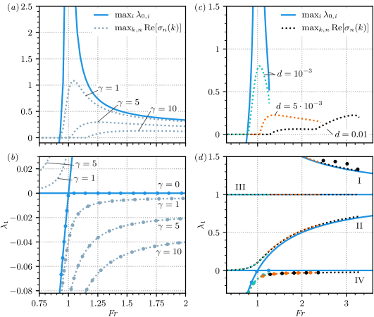
Figure 12: Effect of a bed load flux term on linear growth rates and the corresponding instabilities. Part (a) shows curves of maximum growth rate over all modes and wavenumbers as a function of Fr (dotted), for $\varepsilon=0.01$, $d=0.01$ and various $\gamma=1$, $5$, and $10$ as labelled. Also shown for reference, is the analytical curve of maximum growth rate at high wavenumber (solid blue), for $\gamma=0$. Beneath this, in (b), we plot the system characteristics $\lambda_{1}(\mbox{{Fr}})$ with a solid blue line for $\gamma=0$ and dotted lines for the $\gamma>0$ cases. In the unstable regions, we also plot the corresponding wave speed $c_{\mathrm{max}}(\mbox{{Fr}})$ of the dominant unstable mode at its most unstable wavenumber (filled circles). Part (c) shows maximum growth rate curves, as in (a), for $\varepsilon=6\times 10^{-3}$, $\gamma=8$ and various $d=10^{-3}$ (green dotted), $5\times 10^{-3}$ (orange dotted), $10^{-2}$ (black dotted). The reference curve $\max_{i}\lambda_{0,i}$ (solid blue) is plotted for $\gamma=0$ and $d=10^{-3}$. Underneath, in (d), the characteristics (solid and dotted lines for $\gamma=0$ and $\gamma=8$ respectively) and $c_{\mathrm{max}}(\mbox{{Fr}})$ (filled circles) are plotted using the same colour scheme as (c), with labels I–IV to indicate the corresponding eigenmodes.

The plot may be compared with figure 11(a) and shares the same essential features. This should not be surprising: relatively small values of $\gamma$ do not displace the system characteristics $\lambda_{1}$ far from their resonant values, while larger values push them far apart, leaving little trace of the $\mbox{{Fr}}=1$ singularity. We observe this directly in figure 12(b), which plots $\lambda_{1}(\mbox{{Fr}})$ for each $\gamma$, as labelled (solid and dotted lines), using the same horizontal axes. These curves are obtained by numerically solving (20). The solid lines are the characteristics $\lambda_{1}=1-\mbox{{Fr}}^{-1}$ (mode II) and $\lambda_{1}=0$ (mode IV) of the system without bed load, as derived in (21). As $\gamma$ increases from zero, the curves diverge from the singular intersection point of these two characteristics. Typical values of $\gamma$ from the fluvial literature are $O(10)$ (see e.g. Cordier et al., 2011), around the upper end of the range considered here. In this regime, growth rates are relatively modest and the onset of instability notably increases with $\gamma$, reaching $\mbox{{Fr}}\approx 1.15$, when $\gamma=10$. Where solutions are unstable, we also plot, in figure 12(b), points along $c_{\mathrm{max}}(\mbox{{Fr}})$, which we define here to be the wave speed $c=-\Imag(\sigma)/k$ of the dominant unstable mode at its most unstable wavenumber, i.e. the mode (for each $\gamma$) whose corresponding growth rates are in figure 12(a). Each set of points lies exactly on its corresponding characteristic curve. This is because, in this case, the maximum growth at each Fr occurs in the high-$k$ regime and $c\to\lambda_{1}$ as $k\to\infty$. Furthermore, we note that since $c_{\mathrm{max}}<0$ for $\gamma>0$, dominant perturbations travel upslope (and do so more rapidly if the bed load strength is larger). When $\gamma=10$, the picture in figures 12(a,b) shares traits with some fluvial systems – there is neither ill posedness, nor severely accentuated growth near unit Froude number, and the morphodynamics drives slowly upstream-migrating bedforms (see e.g. Colombini & Stocchino, 2008; Seminara, 2010). It is tempting to think of the morphodynamic processes in this regime as being essentially ‘bed load dominant’. However, pure bed load formulations do not feature instabilities near $\mbox{{Fr}}=1$ (Lanzoni et al., 2006). Indeed, we have checked that decreasing $\varepsilon$ to $10^{-4}$ (and retaining $\gamma=10$), removes the morphodynamic instability in our model, which then remains stable until the threshold for roll waves, near $\mbox{{Fr}}=2$. Therefore, the bulk mass transfer term (i.e. suspended load) plays a role in sustaining the instabilities of figure 12(a).

Furthermore, even if $\gamma$ is large enough that the characteristics are well separated, it is possible to see the influence of the $\mbox{{Fr}}=1$ singularity if we move to a regime where suspended load is enhanced. In figure 12(c), we fix $\gamma=8$, $\varepsilon=6\times 10^{-3}$ and plot maximum growth rate curves, in the vein of figure 12(a), for different $d=0.01$, $5\times 10^{-3}$ and $10^{-3}$. Also shown for reference is the singular high-$k$ growth curve (solid blue), for $d=10^{-3}$ and no bed load. Note that these curves may only be plotted for Fr where steady flows exist and this range shrinks as $d$ decreases. (This is because smaller particles are more easily eroded, meaning that the unsteady scenario of figure 4, where erosion always exceeds deposition, occurs at lower Fr.) The trend of figure 12(c) shows that decreasing particle size leads to more severe growth near $\mbox{{Fr}}=1$, with the $d=10^{-3}$, $\gamma=8$ case (dotted green) inheriting a severe instability in this region. The corresponding characteristics, plotted in figure 12(d) below, are not greatly affected by changes in $d$. Therefore, enhanced growth around unit Froude number cannot be due to near intersection of characteristics in this case. Without simple analytical expressions for the growth rates when $Q\neq 0$, it is difficult to pin down exactly why small $d$ has this effect. However, we note that since our closures for erosion and bed load, given in (51) and (53) respectively, have similar dependencies on the excess shear stress, it is straightforward to see for any given Fr, that $Q/E\propto d\gamma/\varepsilon$. Therefore, smaller $d$ implies that the magnitude of bed load is diminished, relative to the suspended load dynamics.

Finally, just as we saw in figure 12(b), we note that for the $d=10^{-3}$ and $d=5\times 10^{-3}$ case, $c_{\mathrm{max}}$ (filled circles) lies exactly on the characteristic curves corresponding to slowly upstream-propagating disturbances. However, for the $d=0.01$ branch, this mode is only dominant for Froude numbers up to approximately $2.4$, where the rapidly downstream-propagating perturbations of mode I become the most unstable. This is marked in figure 12(c) by a steepening of the maximum growth rate curve and may be compared to the curves in figures 8(a–d), which depict an analogous transition between modes IV and I in the $Q=0$ setting. The latter mode is related to hydraulic roll wave instability, as discussed in §4.5. Note that in this region ($\mbox{{Fr}}\gtrsim 2.4$), $c_{\mathrm{max}}$ does not precisely follow the mode I characteristic. This is because, as in figure 8, maximum growth occurs at finite $k$, rather than in the asymptotic regime where disturbance wave speeds are given exactly by the characteristics.

4.8 Summary

Finally, we return to the unregularised suspended load model and explore the $(d,\mbox{{Fr}})$-parameter space more broadly, by computing the steady states that can exist and their linear stability, when the solid diameter $d$ is varied over three decades. We assume here that the non-dimensional settling speed is constant and unity (as in table 1) throughout, even though its dimensional counterpart $\tilde{w}_{s}$ varies considerably with the particle size. This is reasonable for sufficiently large particles, since $\tilde{w}_{s}\approx\tilde{u}_{p}$, when the particle Reynolds number is high. (This is straightforward to confirm from typical empirical formulae for $\tilde{w}_{s}$, see e.g. Cheng, 1997; Soulsby, 1997). Figure 13 summarises the existence of (a) dilute and (b) concentrated steady flows across parameter space.

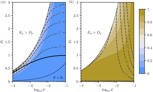
Figure 13: Existence and stability of uniform steady layers in the morphodynamic case. Plotted on two axes are filled contours of scaled solid fraction $\psi$ (shaded regions) for the (a) dilute and (b) concentrated solution branches, over a representative range of $d$ and Fr values. The region where steady erosive flows exist is outlined by dotted black lines. Where no steady flows exist, the plot is left blank. The dilute states possesses a region of stability; the corresponding neutral curve is shown as a solid black line in (a). Overlaid dashed contours indicate lines of constant slope angle.

Where steady solutions exist, we contour them according to $\psi_{0}$. Elsewhere, we leave the region blank. Overlaid are contours showing lines of constant slope angle. Care must be taken when interpreting this plot, since its values depend on the choice of parameters. However, its qualitative characteristics are robust. The most striking observation is the separation of the two states, which are either highly dilute or highly granular. This is clear from considering the picture in figure 4. Solutions exist predominantly for higher $d$, where erosion rates are typically smaller and may therefore balance deposition at higher Fr. As Fr increases, keeping $d$ fixed, eventually $E_{p}>D_{p}$ and states can no longer be steady. Bounding the region of existence from above is the unidimensional family of states of type (b) in figure 4, where the dilute and concentrated branches coalesce. Consequently, the dilute and concentrated states respectively possess greater and lesser solid fractions close to this boundary than they do in the bulk of parameter space. On the dilute contour map, figure 13(a), we also plot the neutral stability curve (solid black), below which states are stable to both hydraulic and morphodynamic modes of disturbance. It is determined (for our chosen closures) by the asymptotic growth rate $\lambda_{0,2}$ (which diverges to $+\infty$ at $\mbox{{Fr}}=1$) crossing zero. Therefore, we compute it by numerically solving $f_{-}(\mbox{{Fr}})=0$, where $f_{-}$ was given in (26). As indicated by figure 7(a), the upper stability limit lies just below the line $\mbox{{Fr}}=1$ for larger $d$ values. At smaller $d$, the neutral line dips as it approaches the existence boundary where solutions are more concentrated. For the parameters used herein, the region of stability includes only extremely shallow grades (typically less than $1^{\circ}$). However, this is not unexpected, since fluid drag predominates and purely Chézy layers turn supercritical (in this case) when $\phi=\arctan(C_{d})\approx 0.6^{\circ}$. Beneath the region where stable dilute erosive flows exist is a region where flows are not sufficiently energetic to entrain material, $\theta<\theta_{c}$, indicated by a dotted line. Here, only steady flows with zero solid fraction exist. In the concentrated case, this region is only very narrow. Note that for any $d$, the limiting solutions as $\mbox{{Fr}}\to 0$ on this branch are static granular layers resting at the neutral slope angle $\arctan(\mu_{1})\approx 5.7^{\circ}$ [see (50) for the definition of $\mu_{1}$]. Such states typically have high Shields numbers in excess of the constant part $\theta_{c}^{*}$ of the critical value and consequently any increase in Fr from zero leads to entrainment. The remainder of parameter space in the concentrated case features steady flows at a range of more severe slope angles, all of which are unstable.

5 Discussion

This study considered the linear response of spatially uniform steady flows on constant slopes to small disturbances, in a general class of morphodynamic shallow-layer models. Our particular interest was situations where there is significant entrainment of bed material (assumed to be a saturated mixture of monodisperse sediment) into the bulk of the flow. We therefore focussed on obtaining results for models developed over the past two decades to describe various highly erosive events such as violent dam failures, flash floods and volcanic lahars. These models augment classical shallow-layer formulations used in hydraulic engineering by accounting for density variations in the flowing mixture, the dynamics of solid transport and the complex processes of exchange between bed and bulk. While they do not typically include a separate bed load – a distinguished layer that transports sediment along the bed surface (as depicted in figure 1), we included such a term at various stages to connect our work with the wider literature on fluvial modelling. Analysis was performed on a generic set of governing equations that may be adapted to specific models by specifying (or omitting) particular closures.

When entrainment of bed material is significant, the stability picture becomes substantially modified, compared with past hydraulic analyses (e.g. Trowbridge, 1987), due to the presence of two extra modes of instability and complicated coupling relationships between hydraulic and morphodynamic feedbacks. For the suspended load model (negligible bed load), we derived analytical formulae for the growth rates of normal mode disturbances in the limits of low and high wavenumber $k$. Most importantly, we observed that the bed evolution equation gives rise to a zero characteristic wave speed that inevitably intersects with one of the hydraulic characteristics at $\mbox{{Fr}}=1$, leading to singularities in the asymptotic (high-$k$) linear growth rates, as observed in figure 7. Existence of these singularities implies two important consequences. Firstly, that these models feature a morphodynamic instability that occurs slightly below unit Froude number. Secondly, and more seriously, that the governing equations are ill posed as initial value problems at $\mbox{{Fr}}=1$, since they permit spatial disturbances to grow arbitrarily rapidly in the limit $k\to\infty$.

Ill posedness is a critical problem for numerical simulations that must always be addressed. However, efforts to solve such models may nonetheless yield plausible results that match observed properties of real flows. This is because the effects of numerical discretisation can make it difficult to identify ill posedness from isolated results, since the length scales over which severe disturbances might develop and grow are limited by spatial resolution. The key indication is that reference solutions cannot be converged in an ill-posed system, since finer grid scales only serve to make the discrete system increasingly sensitive to numerical errors (see Woodhouse et al., 2012, for an example of a resolution-dependent fingering instability in an ill-posed granular flow model). Since erosional shallow flow models with solids transport are needed in critical applications such as hydraulic engineering and natural hazard assessment, it is vital that their numerical solutions are robust. Consequently, operational codes that simulate only the basic suspended load model should be avoided.

In §3.3, we proved that the inclusion of a simple turbulence closure (eddy viscosity) suffices to remove ill posedness from the suspended load model. It is therefore tempting to recommend that the equations should always be regularised with at least a small amount of eddy viscosity. However, even a small amount of diffusion changes the fundamental structure of the model equations and may make them more difficult to time step in a numerical code. Nevertheless, at least one study (within our general framework) includes this term (Simpson & Castelltort, 2006). Moreover, we might anticipate that other turbulence closures, or analogous diffusive terms such as those employed in recent shallow granular flow models (Gray & Edwards, 2014), similarly avoid ill posedness by damping growth in the short-wave limit. As shown in §4.6, the morphodynamic instability near $\mbox{{Fr}}=1$ persists when the model is regularised by eddy viscosity and its onset is unaffected if the regularising term is small. However, figure 11 demonstrated that the magnitude of the eddy viscosity has a significant impact on the severity of this instability. Therefore, selection and calibration of a suitable diffusive closure is far from arbitrary, since it could dictate whether instabilities are seen over the finite lifetime of a simulated geophysical flow. A full investigation of such terms would require careful comparisons with experimental or observed flows.

The removal of ill posedness, through the introduction of eddy viscosity or bed load flux (as in §4.7 and discussed below), does not imply removal of the associated morphodynamic instability that arises near $\mbox{{Fr}}=1$. We have not speculated much about the physics of this instability in the main body of the paper. It may be that it is a purely artificial phenomenon, whose relevance disappears when models are properly calibrated and include all physically important processes. However, in the extended analyses of our illustrative closures, including the eddy viscosity and bed load terms, we were not able to rule out the destabilising influence of the $\mbox{{Fr}}=1$ singularity. Hence, both the severity of its growth and its presence at modest Froude numbers ($\mbox{{Fr}}\gtrsim 1$), make it a feature that should be carefully considered when employing these models. Since the morphodynamic instability exists essentially due to a resonance between the free surfaces of the flow and the bed at short wavelengths, its early development should feature rapid growth of fine scale structure in these fields. Indeed, the growth of mode IV is typically dominant – its components in the asymptotic limit, given by the final vector in (22), couple high frequency oscillations in $h$, $u$ and $b$. To precisely confirm the onset of this instability in a concentrated geophysical flow or a relevant experimental set-up would be challenging. Moreover, while similar resonances have been studied in morphodynamic potential flow models, the resulting instabilities were found to disappear when more detailed physical models were employed (Coleman & Fenton, 2000; Colombini & Stocchino, 2005). However, regardless of these uncertainties, a detailed understanding of the morphodynamic instability is required in order to make properly informed modelling decisions and may be used to guide future model development.

An important next step would be to investigate how the instability develops beyond the linear regime. This could be assessed by conducting a careful nonlinear analysis in the vein of Needham & Merkin (1984), or via carefully resolved numerical simulations of a suitably regularised system. As observed in §4.5, the associated suspended load dynamics acts to suppress the growth rate of mode I, which is responsible for roll wave instability in the hydraulic limit. On this basis, we speculate that the morphodynamic instability may not ultimately cause the flow to roll up into large free-surface waves. Instead, it seems more closely related to an upstream-propagating bedform instability discovered by Balmforth & Vakil (2012) in a simplified model, where $\Gamma$ is assumed to be negligible in all but the bed equation and $Q=0$. This formulation also suffers a singularity at $\mbox{{Fr}}=1$, unless turbulent momentum diffusion is included. The eddy viscosities used to regularise their system were $\nu\sim 10^{-2}$ to $10^{-1}$ – large enough to subdue any dramatic short-wave growth arising from the singularity. However, when $\nu=10^{-2}$, our formulation is nonetheless morphodynamically unstable for all $\mbox{{Fr}}\gtrsim 1.05$ (see figure 11). Moreover, an illustrative numerical calculation (not shown) indicates that it is indeed the mode associated with the bedform that turns unstable (consistent with the role of mode IV elsewhere), with slow upstream-directed phase speed ($c=-0.021$ for the most unstable mode, when $\mbox{{Fr}}=1.2$). It seems reasonable to expect that lower effective turbulent viscosities will be present in at least some natural morphodynamic systems. (See the discussion closing §4.6 for an estimate of the range of $\nu$.) Whether or not this leads to the more severe instabilities predicted by some of our results remains to be established.

Bed load is an important physical process whose inclusion, via a flux term $Q$ in the basal dynamics equation (3c), modifies the characteristic wave speeds of the governing equations. It therefore plays a key role in determining whether the model is strictly hyperbolic (and consequently well posed) or not. This is already well appreciated in models of river morphodynamics, where bed load fluxes are frequently employed and the case for one or more sediment transport layers near the bed surface is experimentally and observationally clear. Consequently, a number of recent studies have investigated conditions for well posedness in these settings (Cordier et al., 2011; Stecca et al., 2014; Chavarrías et al., 2018, 2019). Conversely, models of shallow highly concentrated suspensions rarely include a bed load, since these flows are typically feature an energetic and well-mixed bulk. However, a better approach may be to consider flows on a continuum, from a dilute bed load regime to highly concentrated suspensions. While increasing Shields number causes more grains to be carried into suspension, it seems unreasonable to conclude that $Q$ ultimately shuts off and the bed characteristic becomes zero. Therefore, it may always be prudent to include a bed flux term, in order to avoid potentially artificial resonance between the hydraulic and morphodynamic modes. Such models could easily be checked against the criterion derived in (48) to ensure that they are well posed.

An investigation of the effects of bed load with example model closures in §4.7 demonstrated that its effect on growth rates is similar to that of eddy viscosity – it mollifies the acute growth rates around the $\mbox{{Fr}}=1$ singularity and increases the critical Fr for instability. Our results in figure 12 suggest that both the severity and dominant mode of instability are determined through competition between the morphodynamics of the suspended and bed loads. Indeed, since morphodynamic instabilities are not present near $\mbox{{Fr}}=1$ in pure bed load models (Lanzoni et al., 2006), the effect of mass transfer with the suspended load appears to be destabilising. The predicted instabilities in the $1\lesssim\mbox{{Fr}}\lesssim 2$ region migrate slowly upstream. This is in qualitative agreement with fluvial models that do not employ the shallow flow approximation (see amongst others, Engelund, 1970; Colombini, 2004; Colombini & Stocchino, 2008; Seminara, 2010). These models capture a richer variety of pattern-forming instabilities than appear to be accessible to shallow formulations, such as the formation of dunes for $\mbox{{Fr}}<1$ and various other features (Richards, 1980; Seminara, 2010; Colombini & Stocchino, 2011). Nevertheless, it is interesting that the combined (bed and suspended load) formulation exhibits some morphodynamic instabilities.

Finally, in §4.2 we demonstrated, that steady morphodynamic layers (when they exist) bifurcate into two coexistent states: dilute stable layers and concentrated unstable layers. This is a basic physical idea that lies apart from issues of model consistency and is largely independent of the model closures. In essence, the solutions arise due to the effects of hindered settling, which render the deposition rate non-monotonic with respect to the bulk solid fraction. This means that there are two possible sediment concentrations where erosion exactly balances deposition. Above a certain threshold of Fr, both states cease to exist, since erosion everywhere exceeds the maximal rate of deposition. For the most part, simple physical arguments suffice to explain the stability of the two branches (see §4.2 and 4.3), as we were able to confirm via careful analysis of the linear growth rates in §4.3. This general picture appears to accord with observations of natural flows. Both natural and laboratory debris flows often propagate as an unsteady surge-like front followed by a shallow stable layer of weaker sediment concentration, with this configuration repeating during the flow (Davies et al., 1992; Zanuttigh & Lamberti, 2007; Doyle et al., 2010). For instance, flows of volcanic debris (lahars) typically propagate as alternating debris-rich pulses and relatively shallower and less concentrated ($\sim 20\%$ by volume solids concentration) layers (Pierson, 2005; Doyle et al., 2010). Previous studies have used linear stability analysis to explore the link between flow instabilities such as roll waves and the development of pulses in debris flows (e.g. Zanuttigh & Lamberti, 2007). Further study including fully nonlinear analysis of morphodynamic shallow-layer models, is needed in order to properly link the mechanisms in this paper with observations of natural flows and provides an interesting opportunity for future research.

References

- Ancey (2001) Ancey, C. 2001 Debris flows and related phenomena. In Geomorphological Fluid Mechanics (ed. N. J. Balmforth & A. Provenzale), chap. 21, pp. 528–547. Springer.
- Balmforth & Mandre (2004) Balmforth, N. J. & Mandre, S. 2004 Dynamics of roll waves. J. Fluid Mech. 514, 1–33.
- Balmforth & Vakil (2012) Balmforth, N. J. & Vakil, A. 2012 Cyclic steps and roll waves in shallow water flow over an erodible bed. J. Fluid Mech. 695, 35–62.
- Baloga & Bruno (2005) Baloga, S. M. & Bruno, B. C. 2005 Origin of transverse ridges on the surfaces of catastrophic mass flow deposits on the Earth and Mars. J. Geophys. Res.-Planet. 110 (E5), e05007.
- Benkhaldoun et al. (2011) Benkhaldoun, F., Seaïd, M. & Sahmim, S. 2011 Mathematical development and verification of a finite volume model for morphodynamic flow applications. Adv. Appl. Math. Mech. 3 (4), 470–492.
- Bohorquez & Ancey (2015) Bohorquez, P. & Ancey, C. 2015 Stochastic-deterministic modeling of bed load transport in shallow water flow over erodible slope: Linear stability analysis and numerical simulation. Adv. Water Res. 83, 36–54.
- Cao et al. (2006) Cao, Z., Pender, G. & Carling, P. 2006 Shallow water hydrodynamic models for hyperconcentrated sediment-laden floods over erodible bed. Adv. Water Resour. 29 (4), 546–557.
- Cao et al. (2004) Cao, Z., Pender, G., Wallis, S. & Carling, P. 2004 Computational dam-break hydraulics over erodible sediment bed. J. Hydraul. Eng. 130 (7).
- Cao et al. (2017) Cao, Z., Xia, C., Pender, G. & Liu, Q. 2017 Shallow water hydro-sediment-morphodynamic equations for fluvial processes. J. Hydraul. Eng. 143 (5), 02517001.
- Chang et al. (2000) Chang, H.-C., Demekhin, E. A. & Kalaidin, E. 2000 Coherent structures, self-similarity, and universal roll wave coarsening dynamics. Phys. Fluids 12 (9), 2268–2278.
- Chavarrías et al. (2019) Chavarrías, V., Schielen, R., Ottevanger, W. & Blom, A. 2019 Ill posedness in modelling two-dimensional morphodynamic problems: effects of bed slope and secondary flow. J. Fluid Mech. 868, 461–500.
- Chavarrías et al. (2018) Chavarrías, V., Stecca, G. & Blom, A. 2018 Ill-posedness in modeling mixed sediment river morphodynamics. Adv. Water Res. 114, 219–235.
- Cheng (1997) Cheng, N.-S. 1997 Simplified settling velocity formula for sediment particle. J. Hydraul. Eng. 123 (2), 149–152.
- Coleman & Fenton (2000) Coleman, S. E. & Fenton, J. D. 2000 Potential-flow instability theory and alluvial stream bed forms. J. Fluid Mech. 418, 101–117.
- Colombini (2004) Colombini, M 2004 Revisiting the linear theory of sand dune formation. J. Fluid Mech. 502, 1.
- Colombini & Stocchino (2005) Colombini, M. & Stocchino, A. 2005 Coupling or decoupling bed and flow dynamics: fast and slow sediment waves at high froude numbers. Phys. Fluids 17 (3), 036602.
- Colombini & Stocchino (2008) Colombini, M. & Stocchino, A. 2008 Finite-amplitude river dunes. J. Fluid Mech. 611, 283.
- Colombini & Stocchino (2011) Colombini, M. & Stocchino, A. 2011 Ripple and dune formation in rivers. J. Fluid Mech. 673, 121.
- Cordier et al. (2011) Cordier, S., Le, M. H. & Morales de Luna, T. 2011 Bedload transport in shallow water models: Why splitting (may) fail, how hyperbolicity (can) help. Adv. Water Res. 34 (8), 980–989.
- Cornish (1934) Cornish, V. 1934 Ocean waves and kindred geophysical phenomena. Cambridge University Press.
- Coussot (1994) Coussot, P. 1994 Steady, laminar, flow of concentrated mud suspensions in open channel. J. Hydraul. Res. 32 (4), 535–559.
- Craya (1952) Craya, A. 1952 The criterion for the possibility of roll-wave formation. In Gravity Waves, pp. 141–151. NBS.
- Davies et al. (1992) Davies, T. R., Phillips, C. J., Pearce, A. J. & Zhang, X. B. 1992 Debris flow behaviour—an integrated overview. In Erosion, Debris Flows and Environment in Mountain Regions, , vol. 209, pp. 217–225. IAHS Publ.
- Davies (1986) Davies, T. R. H. 1986 Large debris flows: a macro-viscous phenomenon. Acta Mech. 63 (1-4), 161–178.
- Doyle et al. (2010) Doyle, E. E., Cronin, S. J., Cole, S. E. & Thouret, J.-C. 2010 The coalescence and organization of lahars at Semeru volcano, Indonesia. B. Volcanol. 72 (8), 961–970.
- Dressler (1949) Dressler, R. F. 1949 Mathematical solution of the problem of roll-waves in inclined open channels. Commun. Pur. Appl. Math. 2 (2-3), 149–194.
- Dressler & Pohle (1953) Dressler, R. F. & Pohle, F. V. 1953 Resistance effects on hydraulic instability. Commun. Pure Appl. Math. 6 (1), 93–96.
- Engelund (1970) Engelund, F. 1970 Instability of erodible beds. J. Fluid Mech. 42 (2), 225–244.
- Engelund & Fredsøe (1982) Engelund, F. & Fredsøe, J. 1982 Sediment ripples and dunes. Annu. Rev. Fluid Mech. 14 (1), 13–37.
- Farr & Groot (2009) Farr, R. S. & Groot, R. D. 2009 Close packing density of polydisperse hard spheres. J. Chem. Phys. 131 (24), 244104.
- Forterre & Pouliquen (2003) Forterre, Y. & Pouliquen, O. 2003 Long-surface-wave instability in dense granular flows. J. Fluid Mech. 486, 21–50.
- Gomez (1991) Gomez, B. 1991 Bedload transport. Earth-Sci. Rev. 31 (2), 89–132.
- Gray & Edwards (2014) Gray, J. M. N. T. & Edwards, A. N. 2014 A depth-averaged -rheology for shallow granular free-surface flows. J. Fluid Mech. 755, 503––534.
- Guazzelli & Pouliquen (2018) Guazzelli, É. & Pouliquen, O. 2018 Rheology of dense granular suspensions. J. Fluid Mech. 852, P1.
- Hogg & Pritchard (2004) Hogg, A. J. & Pritchard, D. 2004 The effects of hydraulic resistance on dam-break and other shallow inertial flows. J. Fluid Mech. 501, 179–212.
- Hudson & Sweby (2005) Hudson, J. & Sweby, P. K. 2005 A high-resolution scheme for the equations governing 2D bed-load sediment transport. Int. J. Numer. Meth. Fluids 47 (10-11), 1085–1091.
- Hungr (2000) Hungr, O. 2000 Analysis of debris flow surges using the theory of uniformly progressive flow. Earth Surf. Proc. Land. 25 (5), 483–495.
- Hungr et al. (2005) Hungr, O., McDougall, S. & Bovis, M. 2005 Entrainment of material by debris flows. In Debris-flow hazards and related phenomena, pp. 135–158. Springer.
- Hwang & Chang (1987) Hwang, S.-H. & Chang, H.-C. 1987 Turbulent and inertial roll waves in inclined film flow. Phys. Fluids 30 (5), 1259–1268.
- Iverson (1997) Iverson, R. M. 1997 The physics of debris flows. Rev. Geophys. 35 (3), 245–296.
- Iverson & Ouyang (2015) Iverson, R. M. & Ouyang, C. 2015 Entrainment of bed materials by Earth-surface mass flows: Review and reformulation of depth-integrated theory. Rev. Geophys. 53.
- Iverson et al. (2000) Iverson, R. M., Reid, M. E., Iverson, N. R., LaHusen, R. G., Logan, M., Mann, J. E. & Brien, D. L. 2000 Acute sensitivity of landslide rates to initial soil porosity. Science 290 (5491), 513–516.
- Ivrii & Petkov (1974) Ivrii, V. Y. & Petkov, V. M. 1974 Necessary conditions for the Cauchy problem for non-strictly hyperbolic equations to be well-posed. Russ. Math. Surv. 29 (5), 1.
- Jeffreys (1925) Jeffreys, H. 1925 The flow of water in an inclined channel of rectangular section. Phil. Mag. 49 (293), 793–807.
- Joseph & Saut (1990) Joseph, D. D. & Saut, J. C. 1990 Short-wave instabilities and ill-posed initial-value problems. Theor. Comp. Fluid Dyn. 1 (4), 191–227.
- Juez et al. (2014) Juez, C., Murillo, J. & García-Navarro, P. 2014 A 2D weakly-coupled and efficient numerical model for transient shallow flow and movable bed. Adv. Water Res. 71, 93–109.
- Keulegan & Patterson (1940) Keulegan, G. H. & Patterson, G. W. 1940 A criterion for instability of flow in steep channels. Trans., Am. Geophys. Union 21 (2), 594–596.
- Kozyrakis et al. (2016) Kozyrakis, G. V., Delis, A. I., Alexandrakis, G. & Kampanis, N. A. 2016 Numerical modeling of sediment transport applied to coastal morphodynamics. Appl. Numer. Math. 104, 30–46.
- Lajeunesse et al. (2010) Lajeunesse, E., Malverti, L. & Charru, F. 2010 Bed load transport in turbulent flow at the grain scale: Experiments and modeling. J. Geophys. Res.-Earth 115 (F4).
- Langendoen et al. (2016) Langendoen, E. J., Mendoza, A., Abad, J. D., Tassi, P., Wang, D., Ata, R., El kadi Abderrezzak, K. & Hervouet, J.-M. 2016 Improved numerical modeling of morphodynamics of rivers with steep banks. Adv. Water Resour. 93, 4–14.
- Lanzoni et al. (2006) Lanzoni, S., Siviglia, A., Frascati, A. & Seminara, G. 2006 Long waves in erodible channels and morphodynamic influence. Water Resour. Res. 42 (6).
- Li & Duffy (2011) Li, S. & Duffy, C. J. 2011 Fully coupled approach to modeling shallow water flow, sediment transport, and bed evolution in rivers. Water Resour. Res. 47 (3).
- Liu & Mei (1994) Liu, K. & Mei, C. C. 1994 Roll waves on a layer of a muddy fluid flowing down a gentle slope—a Bingham model. Phys. Fluids 6 (8), 2577–2590.
- Liu & Beljadid (2017) Liu, X. & Beljadid, A. 2017 A coupled numerical model for water flow, sediment transport and bed erosion. Comput. Fluids 154, 273–284.
- Liu et al. (2015) Liu, X., Infante S., Julio Á. & Mohammadian, A. 2015 A coupled two-dimensional numerical model for rapidly varying flow, sediment transport and bed morphology. J. Hydraul. Res. 53 (5), 609–621.
- Lyn (1987) Lyn, D. A. 1987 Unsteady sediment-transport modeling. J. Hydraul. Eng. 113 (1), 1–15.
- Lyn & Altinakar (2002) Lyn, D. A. & Altinakar, M. 2002 St. Venant–Exner equations for near-critical and transcritical flows. J. Hydraul. Eng. 128 (6), 579–587.
- Macedonio & Pareschi (1992) Macedonio, G. & Pareschi, M. T. 1992 Numerical simulation of some lahars from Mount St. Helens. J. Volcanol. Geoth. Res. 54 (1-2), 65–80.
- Meyer-Peter & Müller (1948) Meyer-Peter, E. & Müller, R. 1948 Formulas for bed-load transport. In IAHSR 2nd meeting, Stockholm, Appendix 2. IAHR.
- Murillo & García-Navarro (2010) Murillo, J. & García-Navarro, P. 2010 An Exner-based coupled model for two-dimensional transient flow over erodible bed. J. Comput. Phys. 229 (23), 8704–8732.
- Needham & Merkin (1984) Needham, D. J. & Merkin, J. H. 1984 On roll waves down an open inclined channel. P. Roy. Soc. Lond. A Mat. 394 (1807), 259–278.
- Ng & Mei (1994) Ng, C.-O. & Mei, C. C. 1994 Roll waves on a shallow layer of mud modelled as a power-law fluid. J. Fluid Mech. 263, 151–184.
- Pascal (2006) Pascal, J. P. 2006 Instability of power-law fluid flow down a porous incline. J. Non-Newtonian Fluid Mech. 133 (2-3), 109–120.
- Pierson (1986) Pierson, T. C. 1986 Flow behavior of channelized debris flows Mount St. Helens Washington. In Hillslope Processes (ed. A. Abrahams), pp. 269–296. Routledge.
- Pierson (2005) Pierson, T. C. 2005 Hyperconcentrated flow—transitional process between water flow and debris flow. In Debris-flow hazards and related phenomena, pp. 159–202. Springer.
- Pierson & Scott (1985) Pierson, T. C. & Scott, K. M. 1985 Downstream dilution of a lahar: Transition from debris flow to hyperconcentrated streamflow. Water Resour. Res. 21 (10), 1511–1524.
- Pouliquen & Forterre (2002) Pouliquen, O. & Forterre, Y. 2002 Friction law for dense granular flows: application to the motion of a mass down a rough inclined plane. J. Fluid Mech. 453, 133–151.
- Razis et al. (2014) Razis, D., Edwards, A. N., Gray, J. M. N. T. & van der Weele, K. 2014 Arrested coarsening of granular roll waves. Phys. Fluids 26 (12), 123305.
- Richards (1980) Richards, K. J. 1980 The formation of ripples and dunes on an erodible bed. J. Fluid Mech. 99 (3), 597–618.
- Richardson & Zaki (1954) Richardson, J. F. & Zaki, W. N. 1954 Sedimentation and fluidisation. Part 1. Trans. Inst. Chem. Eng. 32.
- Santiso & Müller (2002) Santiso, E. & Müller, E. A. 2002 Dense packing of binary and polydisperse hard spheres. Mol. Phys. 100 (15), 2461–2469.
- Seminara (2010) Seminara, G. 2010 Fluvial sedimentary patterns. Annu. Rev. Fluid Mech. 42, 43–66.
- Simpson & Castelltort (2006) Simpson, G. & Castelltort, S. 2006 Coupled model of surface water flow, sediment transport and morphological evolution. Comput. Geosci. 32 (10), 1600–1614.
- Siviglia et al. (2013) Siviglia, A., Stecca, G., Vanzo, D., Zolezzi, G., Toro, E. F & Tubino, M. 2013 Numerical modelling of two-dimensional morphodynamics with applications to river bars and bifurcations. Adv. Water Res. 52, 243–260.
- Slootman & Cartigny (2020) Slootman, A. & Cartigny, M. J. B. 2020 Cyclic steps: Review and aggradation-based classification. Earth-Sci. Rev. 201, 102949.
- Soulsby (1997) Soulsby, R. 1997 Dynamics of marine sands. Thomas Telford.
- Spearman & Manning (2017) Spearman, J. & Manning, A. J. 2017 On the hindered settling of sand-mud suspensions. Ocean Dynam. 67 (3), 465–483.
- Stecca et al. (2014) Stecca, G., Siviglia, A. & Blom, A. 2014 Mathematical analysis of the Saint-Venant-Hirano model for mixed-sediment morphodynamics. Water Resour. Res. 50 (10), 7563–7589.
- Swartenbroekx et al. (2013) Swartenbroekx, C., Zech, Y. & Soares-Frazão, S. 2013 Two-dimensional two-layer shallow water model for dam break flows with significant bed load transport. Int. J. Numer. Meth. Fluids 73 (5), 477–508.
- Thual et al. (2010) Thual, O., Plumerault, L.-R. & Astruc, D. 2010 Linear stability of the 1D Saint-Venant equations and drag parameterizations. J. Hydraul. Res. 48 (3), 348–353.
- Trowbridge (1987) Trowbridge, J. H. 1987 Instability of concentrated free surface flows. J. Geophys. Res.–Oceans 92 (C9), 9523–9530.
- Woodhouse et al. (2012) Woodhouse, M. J., Thornton, A. R., Johnson, C. G., Kokelaar, B. P. & Gray, J. M. N. T. 2012 Segregation-induced fingering instabilities in granular free-surface flows. J. Fluid Mech. 709, 543–580.
- Wu & Wang (2007) Wu, W. & Wang, S. S. 2007 One-dimensional modeling of dam-break flow over movable beds. J. Hydraul. Eng. 133 (1), 48–58.
- Xia et al. (2010) Xia, J., Lin, B., Falconer, R. A. & Wang, G. 2010 Modelling dam-break flows over mobile beds using a 2D coupled approach. Adv. Water Resour. 33 (2), 171–183.
- Yue et al. (2008) Yue, Z., Cao, Z., Li, X. & Che, T. 2008 Two-dimensional coupled mathematical modeling of fluvial processes with intense sediment transport and rapid bed evolution. Sci. China Ser. G 51 (9), 1427–1438.
- Zanré & Needham (1994) Zanré, D. D. L. & Needham, D. J. 1994 On the hyperbolic nature of the equations of alluvial river hydraulics and the equivalence of stable and energy dissipating shocks. Geophys. Astrophys. Fluid Dyn. 76 (1-4), 193–222.
- Zanuttigh & Lamberti (2004) Zanuttigh, B. & Lamberti, A. 2004 Analysis of debris wave development with one-dimensional shallow-water equations. J. Hydraul. Eng. 130 (4), 293–304.
- Zanuttigh & Lamberti (2007) Zanuttigh, B. & Lamberti, A. 2007 Instability and surge development in debris flows. Rev. Geophys. 45 (3), rG3006.
- Zayko & Eglit (2019) Zayko, J. & Eglit, M. 2019 Stability of downslope flows to two-dimensional perturbations. Phys. Fluids 31 (8), 086601.