Copas’ method is sensitive to different mechanisms of publication bias

Abstract

Copas’ method corrects a pooled estimate from an aggregated data meta-analysis for publication bias. Its performance has been studied for one particular mechanism of publication bias. We show through simulations that Copas’ method is not robust against other realistic mechanisms. This questions the usefulness of Copas’ method, since publication bias mechanisms are typically unknown in practice.

1 Introduction

In an aggregated data (AD) meta-analysis, published effect sizes from similar research studies are collected to determine a precise pooled effect size. When not all executed research studies are published, an AD meta-analysis may lead to a biased estimate. To correct the pooled estimate for this publication bias, various methods have been proposed (Jin et al., 2015; Mueller et al., 2016; Rucker et al., 2011). Selection model approaches implement a conditional or weighted likelihood function for estimation, where the weights are based on the selection mechanism (Hedges and Vevea, 2006). Copas’ selection method (Copas and Shi, 2000, 2001) uses the standard errors of the study effect sizes to create these weights. The method gives a higher weight to studies with a lower probability of being published.

Copas’ method has been compared to the Trim and Fill method (Duval and Tweedie, 2000b, a) using 157 meta-analyses. Even though both methods produced similar point estimates, Copas’ method was preferred since it produced larger standard errors, making Copas’ method somewhat more conservative (Schwarzer et al., 2010). Since direct likelihood-based methods may sometimes suffer from convergence issues, an expectation-maximization (EM) algorithm was developed for Copas’ method (Ning et al., 2017). Furthermore, a Bayesian extension of Copas’ method was developed for network meta-analysis (Mavridis et al., 2013). This all shows the importance of Copas’ method in meta-analysis.

Unfortunately, the performance of Copas’ method has been investigated for one particular mechanism of publication bias using simulation studies, even though other mechanisms for publication bias have been proposed in literature (Stanley, 2008; Stanley and Doucouliagos, 2014; van Aert and van Assen, 2018; Hedges, 1984; McShane et al., 2016). We will demonstrate that Copas’ method is sensitive to these mechanisms when mean differences are being pooled.

Section 2 describes Copas’ method and three mechanisms for publication bias. Section 3 describes our simulation study. The results and the discussion are presented in Sections 4 and 5, respectively.

2 Statistical methods

The information in an AD meta-analysis consists of the pair $(D_{i},S_{i})$ for study $i=1,2,...,m$, where $D_{i}$ is the observed or collected effect size and $S_{i}$ is the accompanied standard error. In some applications there may also exist a degrees of freedom for the standard error (Cochran, 1954), but this is ignored here.

2.1 The Copas method

Copas and Shi (2000, 2001) considered a population of study effect sizes that follow the random effects meta-analysis model

$$D_{i}=\theta+U_{i}+\varepsilon_{i},$$ (1)

with $\theta$ the unknown mean effect size of interest, $U_{i}\sim N(0,\tau^{2})$ the heterogeneity in study effect sizes, and $\varepsilon_{i}\sim N(0,\sigma_{i}^{2})$ the residual independent of $U_{i}$ with an unknown variance $\sigma_{i}^{2}$ that may vary with study. However, they assumed that only a selective subset of all studies has been published and introduce a selection model $Z_{i}=\alpha+\beta S_{i}^{-1}+\delta_{i}$, with $\alpha$ and $\beta$ fixed parameters, $\delta_{i}\sim N(0,1)$ being correlated with $\varepsilon_{i}$, $\rho=\mathsf{CORR}(\varepsilon_{i},\delta_{i})$, and $D_{i}$ only being published when $Z_{i}>0$. Note that studies with smaller standard errors have a higher probability of being published and when $\beta=0$ and $\alpha$ is large, there is no publication bias present.

Based on the population and selection model for effect sizes, a weighted or conditional log likelihood function is constructed

$$\ell\left(\theta,\tau^{2},\rho\right)=\sum_{i=1}^{m}\left[\log p\left(D_{i}|Z_{i}>0,S_{i}\right)\right],$$

with $p\left(D_{i}|Z_{i}>0,S_{i}\right)$ the conditional probability density of an effect size given that the study is selected. Using a joint normality assumption on $(\varepsilon_{i},\delta_{i})$ and assuming that $(\varepsilon_{i},\delta_{i})$ is independent of $U_{i}$, the conditional log likelihood function can be written in the following explicit expression (Copas and Shi, 2000, 2001)

$$\sum_{i=1}^{m}\left[-\tfrac{1}{2}\log\left(\tau^{2}+\sigma_{i}^{2}\right)-\dfrac{(D_{i}-\theta)^{2}}{2(\tau^{2}+\sigma_{i}^{2})}-\log\Phi(\alpha+\beta S_{i}^{-1})+\log\Phi(V_{i})\right],$$ (2)

with $\Phi$ the standard normal distribution function, $V_{i}$ given by $V_{i}=[\alpha+\beta S_{i}^{-1}+\tilde{\rho}_{i}(D_{i}-\theta)/(\tau^{2}+\sigma_{i}^{2})^{1/2}]/[1-\tilde{\rho}_{i}^{2}]^{1/2}$, and $\tilde{\rho}_{i}=\sigma_{i}\rho/[\tau^{2}+\sigma_{i}^{2}]^{1/2}$. The unknown variance $\sigma_{i}^{2}$ in (2) is replaced by $S_{i}^{2}/[1-c_{i}^{2}\rho^{2}]$, with $c_{i}=\lambda(\alpha+\beta S_{i}^{-1})[\alpha+\beta S_{i}^{-1}+\lambda(\alpha+\beta S_{i}^{-1})]$, $\lambda(z)=\phi(z)/\Phi(z)$, and $\phi$ the standard normal density function.

For fixed values of $\alpha$ and $\beta$, the log likelihood function in (2) is maximized over $\theta$, $\tau^{2}$, and $\rho$ and their confidence intervals are based on asymptotic theory. By studying a grid of different values for $\alpha$ and $\beta>0$, such that $0.01\leq P(Z_{i}>0|S_{i})\leq 0.99$ for the smallest and largest value of $S_{i}$, the sensitivity of the pooled estimator $\hat{\theta}$ on $\alpha$ and $\beta$ can be investigated (Copas and Shi, 2000, 2001). Settings for $\alpha$ and $\beta$ for which selection bias is not rejected would fit best with the data. This selection bias is tested with a form of Egger’s test (Egger et al., 1997). The random effects model is extended to $D_{i}=\theta+\gamma S_{i}^{-1}+U_{i}+\varepsilon_{i}$ and $H_{0}:\gamma=0$ is tested with a likelihood ratio test Copas and Shi (2000, 2001); Carpenter et al. (2009). We used the R-package “copas” which is part of the R-package meta to carry out the Copas method Carpenter et al. (2009).

2.2 Selection models

The selection model of Copas is based on the positiveness of the latent variable $Z_{i}=\alpha+\beta S_{i}^{-1}+\delta_{i}$, with $\delta_{i}$ correlated with the residual in the random effect model in (1). However, there may be alternative approaches that would be based on the standardized effect sizes $D_{i}/S_{i}$. Indeed, standardized effect sizes closer to zero would be less likely to be published and large effect sizes (at one side or in one direction) would be more likely to be published (Hedges, 1984).

2.2.1 Significant effect size

Selection models based on the $p$-value of the study effect have been proposed in literature (Stanley, 2008; Stanley and Doucouliagos, 2014; van Aert and van Assen, 2018; Hedges, 1984; McShane et al., 2016). When the effect size is significant (assuming more positive effect sizes), i.e., $D_{i}/S_{i}>z_{1-\alpha}$, with $\alpha$ the significance level and $z_{q}$ the $q$^th quantile of a standard normal distribution, the study is included. To add randomness to the non-significant studies, a uniform distributed random variable $U(0,1)$ and a parameter $\pi_{\mathrm{pub}}$ can be used. If the uniform random variable is smaller than or equal to $1-\pi_{\mathrm{pub}}$, the non-significant study is included too, and otherwise it is excluded.

2.2.2 Standardized effect size

An alternative approach, is to use $D_{i}/S_{i}$ in a selection model similar to Copas’ selection model. Study $i$ is published when the latent variable $Z_{i}=a+bD_{i}/S_{i}+\delta_{i}$ is positive, with $a$ and $b$ fixed parameters, and with $\delta_{i}\sim N\left(0,1\right)$, now being independent of the residual in model (1). We do not need a non-zero correlation between $\delta_{i}$ and $\varepsilon_{i}$, since the correlation with the population effect size or the selection of studies is now directly induced by the standardized effect size. The probability that study $i$ is selected is $P(Z_{i}>0|D_{i}=d,S_{i}=s)=\Phi(a+bd/s)$.

2.3 Simulation model

We will first draw a population of effect sizes and standard errors, i.e., draw pair $(D_{i},S_{i})$, that is calculated from individual participant data (IPD) for two groups in each study. Then we will use the different selection models to eliminate studies from the population.

2.3.1 Population of aggregated data

We consider a meta-analysis with $m$ studies, having sample sizes $n_{i}$, $i=1,\cdots,m$. The number of participants $n_{i}$ for study $i$ is drawn using an overdispersed Poisson distribution with parameter $\lambda$. The value $\gamma_{i}\sim\Gamma\left(a_{0},b_{0}\right)$, with $\Gamma\left(a_{0},b_{0}\right)$ a gamma distribution with parameters $a_{0}$ and $b_{0}$, is drawn to make a study specific parameter $\lambda_{i}=\lambda\exp\left(0.5\gamma_{i}\right)$. Then $n_{i}$ is drawn from a Poisson distribution with parameter $\lambda_{i}$, i.e., $n_{i}\sim\mathrm{Pois}\left(\lambda_{i}\right)$. This sample size is then split in two sample sizes using a Binomial distribution with parameter $p$, i.e., $n_{i0}\sim\mathrm{Bin}(n_{i},p)$ and $n_{i1}=n_{i}-n_{i0}$.

Then a continuous response $Y_{ijk}$ for individual $k(=1,\cdots,n_{ij})$, in group $j(=0,1)$, for study $i(=1,2,...,m)$ is simulated according to a linear mixed model:

$$Y_{ijk}=\mu+\beta_{j}+U_{ij}+\epsilon_{ijk},$$ (3)

with $\mu$ a general mean, $\beta_{j}$ an effect of group $j$ ($\beta_{0}=0$ and $\beta_{1}=\theta$), $U_{ij}$ a study-specific random effect for group $j$, and residual $\epsilon_{ijk}\sim N\left(0,\zeta^{2}\right)$. We assume that $(U_{i0},U_{i1})^{T}$ is bivariate normally distributed with zero means and variance-covariance matrix $\varSigma$ given by

$$\varSigma=\left[\begin{array}[]{cc}\sigma_{0}^{2}&\rho_{01}\sigma_{0}\sigma_{1}\\ \rho_{01}\sigma_{0}\sigma_{1}&\sigma_{1}^{2}\end{array}\right].$$

After simulating the individual responses, the study effect size is calculated by the mean difference $D_{i}=\bar{Y}_{i0.}-\bar{Y}_{i1.}$, with $\bar{Y}_{ij.}=\sum_{i=1}^{n_{ij}}Y_{ijk}/n_{ij}$ the average of group $j$ in study $i$. It is straightforward to see that $D_{i}$ satisfies model (1) with $U_{i}=U_{i0}-U_{i1}\sim N(0,\sigma_{0}^{2}-2\rho_{01}\sigma_{0}\sigma_{1}+\sigma_{1}^{2})$ and $\varepsilon_{i}\sim N(0,\zeta^{2}[n_{i0}^{-1}+n_{i1}^{-1}])$. The standard error $S_{i}$ was estimated using the formula $S_{i}=\sqrt{S_{i0}^{2}/n_{i0}+S_{i1}^{2}/n_{i1}}$, with $S_{ij}^{2}=\sum_{k=1}^{n_{ij}}(Y_{ijk}-\bar{Y}_{ij.})^{2}/(n_{ij}-1)$ the sample variance of group $j$ in study $i$, not assuming that the residual variance in model (3) is homogeneous.

The settings of the parameters are chosen such that the simulation corresponds approximately with a meta-analysis of clinical trials on hypertension treatment. Parameter settings used to generate the aggregated data are $m\in\{30,50,100\}$, $\lambda=100$, $a_{0}=b_{0}=1$, $p=0.5$, $\mu=160$, $\theta=-0.5$, $\zeta^{2}=100$, $\sigma_{0}^{2}\in\{0,2\}$, $\sigma_{1}^{2}\in\{0,3\}$, and $\rho_{01}\in\{0,0.7\}$. We will run all combinations of parameter choices and simulate 1000 meta-analysis studies. Note that this implies that we study five levels of heterogeneity, i.e., $\tau^{2}=\sigma_{0}^{2}-2\rho_{01}\sigma_{0}\sigma_{1}+\sigma_{1}^{2}\in\{0,2,5-1.4\sqrt{6},3,5\}$, but we will only report three levels $\{0,5-1.4\sqrt{6},5\}$. These settings correspond to an intraclass correlation coefficient (ICC) of approximately 0%, 40%, and 68%, respectively, since we expect an average sample size per treatment group to be equal to $85$ individuals.

2.3.2 Selection of studies

Copas’ selection model requires simulation of $Z_{i}=\alpha+\beta S_{i}^{-1}+\delta_{i}$, with $\delta_{i}$ being correlated to $\varepsilon_{i}$ in (1). The residual $\varepsilon_{i}$ can be calculated from the simulation of the individual data, since $\varepsilon_{i}=\bar{\epsilon}_{i0.}-\bar{\epsilon}_{i1.}$, with $\bar{\epsilon}_{ij}=\sum_{k=1}^{n_{ij}}\epsilon_{ijk}/n_{ij}$. Then $\delta_{i}$ can be drawn from a normal distribution

$$\delta_{i}|\bar{\epsilon}_{i0.}-\bar{\epsilon}_{i1.}\sim N\left(\rho[\bar{\epsilon}_{i0.}-\bar{\epsilon}_{i1.}]/\sqrt{\zeta^{2}[n_{i0}^{-1}+n_{i1}^{-1}]},1-\rho^{2}\right),$$

where $\rho=\mathsf{CORR}(\delta_{i},\varepsilon_{i})$ is the correlation parameter taken equal to $\rho\in\{0,0.9\}$. The parameters $\alpha$ and $\beta$ will depend on the simulated population data and vary with each simulation run.

We used the 5% and 95% quantiles of the set of precision estimates $S_{1}^{-1}$, $S_{2}^{-1}$, …, $S_{m}^{-1}$ for one meta-analysis, say $q_{5}$ and $q_{95}$, respectively. The values $\alpha$ and $\beta$ are chosen such that $P(Z_{i}>0|S_{i}^{-1}=q_{95})=0.99$ and $P(Z_{i}>0|S_{i}^{-1}=q_{5})=p_{0}$, with $p_{0}\leq 0.50$. A study with a small standard error is almost always selected, while studies with larger standard errors are more likely eliminated from the meta-analysis. Solving the two equations results in parameters $\alpha\approx(z_{p_{0}}q_{95}-2.33q_{5})/(q_{95}-q_{5})$ and $\beta\approx(z_{p_{0}}-\alpha)/q_{5}$, when the random term $\delta_{i}$ is independent of all other terms. A study $i$ was selected if $Z_{i}>0$, and it was eliminated when $Z_{i}\leq 0$. We tuned the parameter $p_{0}$ such that we select approximately 70% of all simulated studies under the same settings.

Simulation of the selection models based on standardized effect sizes $D_{i}/S_{i}$ are more straightforward. For latent variable $Z_{i}=a+bD_{i}/S_{i}+\delta_{i}$, we draw $\delta_{i}$ from a standard normal distribution, independent of anything else. Here we use $a$ and $b$ in the same way as $\alpha$ and $\beta$, but the quantiles $q_{5}$ and $q_{95}$ are now calculated from the set of standardized effect sizes $D_{1}/S_{1}$, $D_{2}/S_{2}$,…, $D_{m}/S_{m}$ (assuming $D_{i}$’ s are mostly positive, otherwise we could use $-D_{i}/S_{i}$). For the $p$-value based selection of studies, we searched for values of $\pi_{\mathrm{pub}}$ such that approximately 70% of the studies are included.

The average effective number of studies $\bar{m}$ included in the simulations for the three selection models will be reported.

3 Results

Figure 1 shows the distributions of the standardized effect sizes for the selected and non-selected studies for the four selections models ($\sigma_{0}^{2}=2$; $\sigma_{1}^{2}=3$; $\rho_{01}=0$). The mechanisms based on the standardized effect sizes have a stronger effect on selection of studies than Copas’ selection model. The selection model based on $D_{i}/S_{i}$ also show a different mechanism. The $p$-value based selection model shows the truncation of being significant, $Z_{i}=a+bD_{i}/S_{i}+\delta_{i}$ shifts the distribution, while Copas’ selection models essentially eliminate higher standardized effects sizes with lower probabilities.

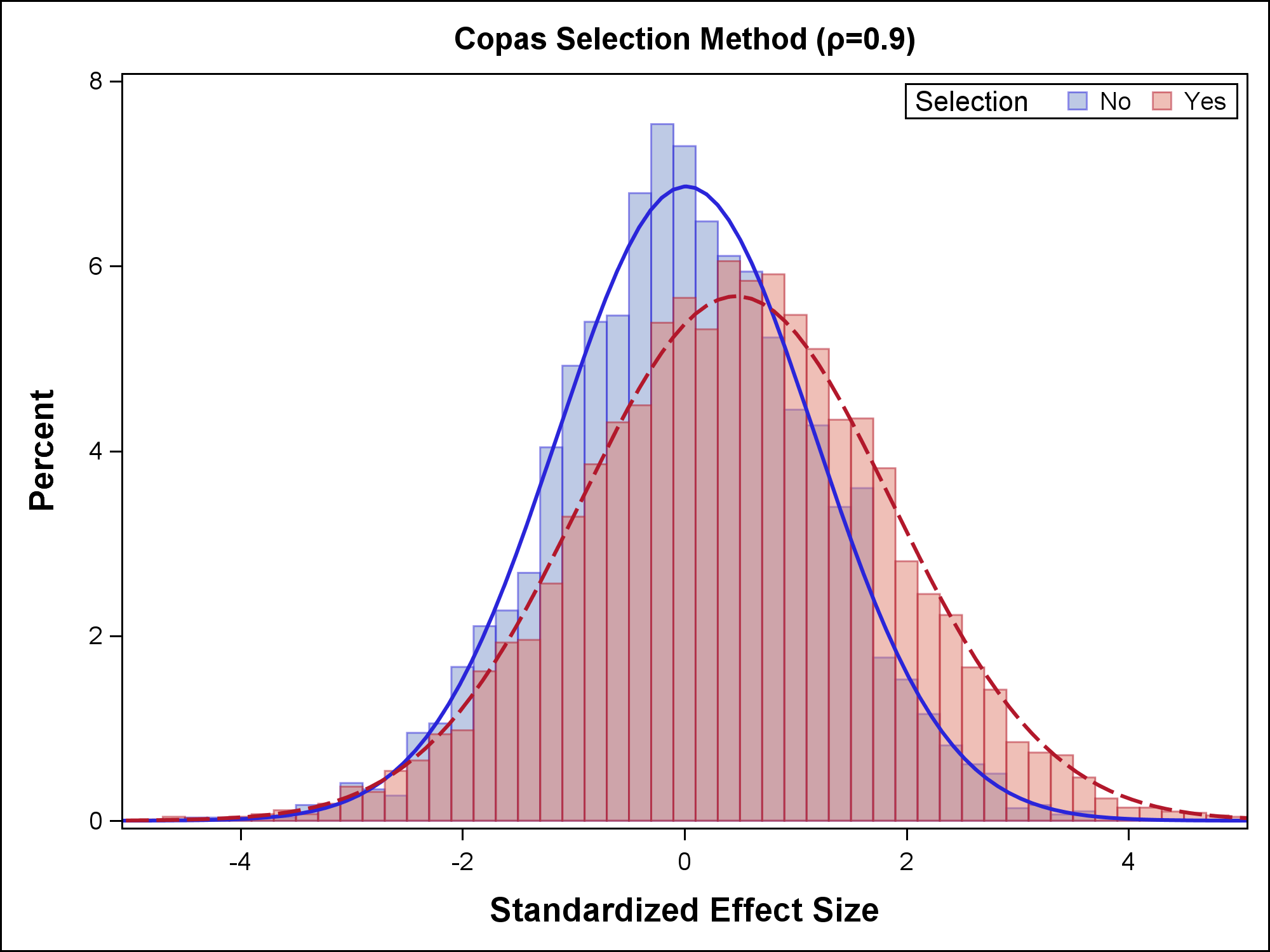
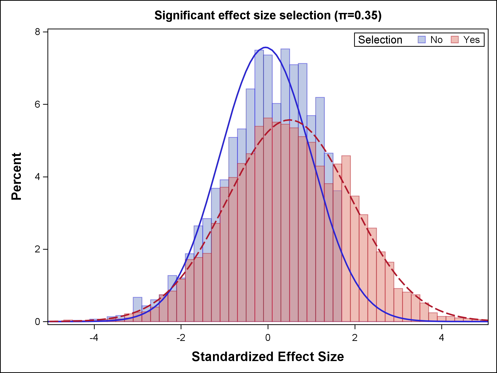
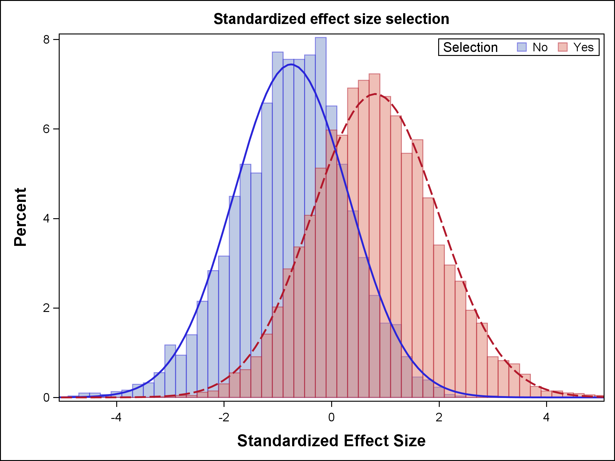
Figure 1: Visualization of the selection of studies for the selection models.

The performance of Copas’ method on estimation of the pooled effect size ($\theta$) for the different selection methods is evaluated with the Mean Squared Error (MSE), the bias, and the coverage probability (CP). The results of the simulations are presented in Table 1 for $m=30$. The results for other numbers of study sizes are very similar to the results of $m=30$.

Table 1: Performance of Copas’ method (MSE, bias and CP(%)) for estimation of the pooled estimate ($\theta=-0.5$; publication rate $\approx 70\%$; $m=30$).

$\sigma_{0}^{2}$	$\sigma_{1}^{2}$	$\rho_{01}$	Selection method		MSE	Bias	CP(%)	$\bar{m}$
0	0	0	Copas	$\rho=0$	0.11645	0.00393	0.943	20.7
0	0	0		$\rho=0.9$	0.14352	-0.04650	0.922	21.1
0	0	0	Significant effect		0.15348	-0.03456	0.924	21.6
0	0	0	Standardized effect		0.33874	-0.45506	0.681	20.7
2	3	0.7	Copas	$\rho=0$	0.28760	-0.01156	0.873	20.7
2	3	0.7		$\rho=0.9$	0.31806	-0.05903	0.858	21.1
2	3	0.7	Significant effect		0.39669	-0.11541	0.875	21.0
2	3	0.7	Standardized effect		0.77575	-0.69885	0.521	20.6
2	3	0	Copas	$\rho=0$	0.50614	-0.00193	0.886	20.7
2	3	0		$\rho=0.9$	0.55830	-0.11847	0.877	21.1
2	3	0	Significant effect		0.67515	-0.14357	0.885	21.3
2	3	0	Standardized effect		1.59896	-1.03069	0.480	20.5

Introducing publication bias according to Copas’ selection model, clearly results in the lowest MSE and bias (as expected). When heterogeneity in study effect sizes increases and when the selection model is correlated to the random effects model ($\rho=0.9$) a bias appears that can reach a level of 20% of the pooled effect size. The coverage probability is in general liberal and only close to nominal for homogeneous study effect sizes. Selection of studies based on significant effect sizes increases the MSE and the bias. For homogeneous study effect sizes, the bias is still limited to approximately 7%, but when heterogeneity is increasing the relative bias can easily increase to approximately 30%. Due to the increased MSE compared to Copas’ selection model, the coverage of the 95% confidence interval remains at the same level as Copas’ selection model. When the selection is based directly on the standardized effect sizes, Copas’ model seem to fail completely, in particular when heterogeneity is present. Copas’ method does not correct the estimate enough, leading to very high biases and low coverage probabilities.

4 Discussion

The purpose of this paper was to investigate the performance of Copas’ method for adjusting the pooled estimate from an aggregated data meta analysis in the presence of publication bias. We focused on effect sizes in the form of mean differences and studied three different selection models for publication bias. These selection models were all (indirectly or directly) related to the effect size of a study (Hedges, 1984; McShane et al., 2016).

Copas’ method overestimates treatment effect (e.g., does not correct enough) in case of between-study heterogeneity, regardless of the selection model. The Copas method performs best and corrects adequately when publication bias follows Copas’ selection model. Our results are comparable to results on bias and coverage in literature (Ning et al., 2017). However, when the mechanism behind publication bias is different from that used in the Copas’ selection model, the method performs rather poorly. This happens in particular when the standardized effect size is the statistic that would drive publication bias. Heterogeneity in study effect sizes emphasizes the shortcomings of Copas’ method.

This paper only considered mean differences, but we do not think that other types of effect sizes (e.g., log odds ratios) would provide any different results. It is very common to assume that other types of effect sizes also follow the random effects model in (1) approximately, i.e., the model we used for our simulations. Additionally, other reasons for publication bias, which we did not study, have been mentioned in literature as well (Sterne et al., 2011), e.g., language bias, availability bias, and cost bias. It is unknown how Copas’ method deals with these forms of biases, but we feel that it is unlikely that Copas’ method corrects appropriately, since these biases are probably not described well by Copas’ selection model. We recommend to improve Copas’ method to make it more robust against different forms of publication bias.

Conflict of Interest

The authors have declared no conflict of interest.

Reference

References

- Carpenter et al. (2009) Carpenter, J., Rücker, G., Schwarzer, G., 2009. copas: An r package for fitting the copas selection model. The R Journal 1 (2), 31.
- Cochran (1954) Cochran, W. G., mar 1954. The combination of estimates from different experiments. Biometrics 10 (1), 101.
- Copas and Shi (2001) Copas, J., Shi, J., aug 2001. A sensitivity analysis for publication bias in systematic reviews. Statistical Methods in Medical Research 10 (4), 251–265.
- Copas and Shi (2000) Copas, J., Shi, J. Q., sep 2000. Meta-analysis, funnel plots and sensitivity analysis. Biostatistics 1 (3), 247–262.
- Duval and Tweedie (2000a) Duval, S., Tweedie, R., mar 2000a. A nonparametric ”trim and fill” method of accounting for publication bias in meta-analysis. Journal of the American Statistical Association 95 (449), 89.
- Duval and Tweedie (2000b) Duval, S., Tweedie, R., jun 2000b. Trim and fill: A simple funnel-plot-based method of testing and adjusting for publication bias in meta-analysis. Biometrics 56 (2), 455–463.
- Egger et al. (1997) Egger, M., Smith, G. D., Schneider, M., Minder, C., sep 1997. Bias in meta-analysis detected by a simple, graphical test. BMJ 315 (7109), 629–634.
- Hedges (1984) Hedges, L. V., mar 1984. Estimation of effect size under nonrandom sampling: The effects of censoring studies yielding statistically insignificant mean differences. Journal of Educational Statistics 9 (1), 61–85.
- Hedges and Vevea (2006) Hedges, L. V., Vevea, J., mar 2006. Selection method approaches. In: Publication Bias in Meta-Analysis. John Wiley & Sons, Ltd, pp. 145–174.
- Jin et al. (2015) Jin, Z.-C., Zhou, X.-H., He, J., nov 2015. Statistical methods for dealing with publication bias in meta-analysis. Statistics in Medicine 34 (2), 343–360.
- Mavridis et al. (2013) Mavridis, D., Sutton, A., Cipriani, A., Salanti, G., jul 2013. A fully bayesian application of the copas selection model for publication bias extended to network meta-analysis. Statistics in Medicine 32 (1), 51–66.
- McShane et al. (2016) McShane, B. B., Böckenholt, U., Hansen, K. T., sep 2016. Adjusting for publication bias in meta-analysis. Perspectives on Psychological Science 11 (5), 730–749.
- Mueller et al. (2016) Mueller, K. F., Meerpohl, J. J., Briel, M., Antes, G., von Elm, E., Lang, B., Motschall, E., Schwarzer, G., Bassler, D., dec 2016. Methods for detecting, quantifying, and adjusting for dissemination bias in meta-analysis are described. Journal of Clinical Epidemiology 80, 25–33.
- Ning et al. (2017) Ning, J., Chen, Y., Piao, J., feb 2017. Maximum likelihood estimation and em algorithm of copas-like selection model for publication bias correction. Biostatistics 18 (3), 495–504.
- Rucker et al. (2011) Rucker, G., Schwarzer, G., Carpenter, J. R., Binder, H., Schumacher, M., jul 2011. Treatment-effect estimates adjusted for small-study effects via a limit meta-analysis. Biostatistics 12 (1), 122–142.
- Schwarzer et al. (2010) Schwarzer, G., Carpenter, J., Rücker, G., mar 2010. Empirical evaluation suggests copas selection model preferable to trim-and-fill method for selection bias in meta-analysis. Journal of Clinical Epidemiology 63 (3), 282–288.
- Stanley (2008) Stanley, T. D., 2008. Meta-regression methods for detecting and estimating empirical effects in the presence of publication selection. Oxford Bulletin of Economics and Statistics 70 (1), 103–127.
- Stanley and Doucouliagos (2014) Stanley, T. D., Doucouliagos, H., sep 2014. Meta-regression approximations to reduce publication selection bias. Research Synthesis Methods 5 (1), 60–78.
- Sterne et al. (2011) Sterne, J. A. C., Sutton, A. J., Ioannidis, J. P. A., Terrin, N., Jones, D. R., Lau, J., Carpenter, J., Rucker, G., Harbord, R. M., Schmid, C. H., Tetzlaff, J., Deeks, J. J., Peters, J., Macaskill, P., Schwarzer, G., Duval, S., Altman, D. G., Moher, D., Higgins, J. P. T., jul 2011. Recommendations for examining and interpreting funnel plot asymmetry in meta-analyses of randomised controlled trials. BMJ 343 (jul22 1), d4002–d4002.
- van Aert and van Assen (2018) van Aert, R. C. M., van Assen, M. A. L. M., oct 2018. Correcting for publication bias in a meta-analysis with the p-uniform* method.