Geometric Total Variation for Image Vectorization, Zooming and Pixel Art Depixelizing

Abstract

We propose an original method for vectorizing an image or zooming it at an arbitrary scale. The core of our method relies on the resolution of a geometric variational model and therefore offers theoretic guarantees. More precisely, it associates a total variation energy to every valid triangulation of the image pixels. Its minimization induces a triangulation that reflects image gradients. We then exploit this triangulation to precisely locate discontinuities, which can then simply be vectorized or zoomed. This new approach works on arbitrary images without any learning phase. It is particularly appealing for processing images with low quantization like pixel art and can be used for depixelizing such images. The method can be evaluated with an online demonstrator, where users can reproduce results presented here or upload their own images.

1 Introduction

There exist many methods for zooming into raster images, and they can be divided into two groups. The first group gathers “image super-resolution” or “image interpolation” techniques and tries to deduce colors on the zoomed image from nearby colors in the original image. These methods compute in the raster domain and their output is not scalable. The second group is composed of “image vectorization” approaches and tries to build a higher level representation of the image made of painted polygons and splines. These representations can be zoomed, rotated or transformed. Each approach has its own merits, but none perform well both on cmaera pictures and on drawings or pixel art.

Image interpolation/super resolution.

These approaches construct an interpolated image with higher resolution. A common trait is that they see the image as a continuous function, such that we only see its sampling in the original image. Their diversity lies generally in the choice of the space of continuous functions. For instance linear/cubic interpolation just fits linear/cubic functions, but much more complicated spaces have been considered. For instance the method proposed by Getreuer introduces the concept of contour stencils [6, 7] to accurately estimate the edge orientation. Roussos and Maragos proposed another strategy using a tensor driven diffusion [19] (see also [8]).

Due to the increasing popularity of convolutional neural network (CNN), several authors propose super resolution networks to obtain super resolution image. For instance Shi et al. define a CNN architecture exploiting feature maps computed in low resolution space [22]. After learning, this strategy reduces the computational complexity for a fixed super-resolution and gives interesting results on photo pictures. Of course, all these approaches do not provide any vectorial representation and give low quality results on images with low quantization or pixel art images. Another common feature is their tendency to “invent” false oscillating contours, like in Fourier super-resolution.

Pixel art super-resolution. A subgroup of these methods is dedicated to the interpolation of pixel art images, like the classic $HqX$ magnification filter [23] where $X$ represents the scale factor. We may quote a more advanced approach which proposes as well a full vectorization of pixel art image [13]. Even if the resulting reconstruction for tiny images is nice looking, the proposed approach is designed specifically for hand-crafted pixel art image and is not adaptable to photo pictures.

Image vectorization. Recovering a vector-based representation from a bitmap image is a classical problem in the field of digital geometry, computer graphics and pattern recognition. Various commercial design softwares propose such a feature, like Indesign™, or Vector Magic [10] and their algorithms are naturally not disclosed. Vectorization is also important for technical document analysis and is often performed by decomposition into arcs and straight line segments [9]. For binary images, many vectorization methods are available and may rely on dominant points detection [16, 17], relaxed straightness properties [1], multi-scale analysis [5] or digital curvature computation [11, 15].

Extension to grey level images is generally achieved by image decomposition into level sets, vectorization of each level, then fusion (e.g. [12]). Extension to color images is not straightforward. Swaminarayan and Prasad proposed to use contour detection associated to a Delaunay triangulation [25] but despite the original strategy, the digital geometry of the image is not directly exploited like in above-mentionned approaches. Other methods define the vectorization as a variational problem, like Lecot and Levy who use the Mumford Shah piecewise smooth model and an intermediate triangulation step to best approximate the image [14]. Other comparable methods construct the vectorization from topological preservation criteria [24], from splines and adaptive Delaunay triangulation [4] or from Bézier-curves-patch-based representation [26]. We may also cite the interactive method proposed by Price and Barrett that let a user edit interactively the reconstruction from a graph cut segmentation [18].

Our contribution. We propose an original approach to this problem, which borrows and mixes techniques from both groups of methods, thus making it very versatile. We start with some notations that will be used thoughout the paper. Let $\Omega$ be some open subset of $\mathbb{R}^{2}$, here a rectangular subset defining the image domain. Let $K$ be the image range, a vector space that is generally $\mathbb{R}$ for monochromatic images and $\mathbb{R}^{3}$ for color image, equipped with some norm $\left\|\cdot\right\|_{K}$. We assume in the following that gray-level and color components lie in $[0,1]$.

First our approach is related with the famous Total Variation ($\mathrm{TV}$), a well known variational model for image denoising or inpainting [20]. Recall that if $f$ is a differentiable function in $\Omega$, its total variation can be simply defined as:

$$\mathrm{TV}(f):=\int_{\Omega}\left\|\nabla f(x)\right\|_{K}\mathrm{d}x.$$ (1)

In a more general setting, the total variation is generally defined by duality. As noted by many authors [3], different discretizations of $\mathrm{TV}$ are not equivalent. However they are all defined locally with neighboring pixels, and this is why they are not able to fully capture the structure of images.

In Section 2, we propose a geometric total variation. Its optimization seeks the triangulation of lattice points of $\Omega$ that minimizes a well-defined $\mathrm{TV}$ corresponding to a piecewise linear function interpolating the image. The optimal triangulation does not always connect neighboring pixels and align its edges with image discontinuities. For instance digital straight segments are recognized by the geometric total variation.

In Section 3, we show how to construct a vector representation from the obtained triangulation, by regularizing a kind of graph dual to the triangulation. Section 4 shows a super-resolution algorithm that builds a zoomed raster image with smooth Bezier discontinuities from the vector representation. Finally, in Section 5 we compare our approach to other super-resolution and vectorization methods and discuss the results.

2 Geometric Total Variation

The main idea of our geometric total variation is to structure the image domain into a triangulation, whose vertices are the pixel centers located at integer coordinates. Furthermore, any triangle of this triangulation should cover exactly three lattice points (its vertices). The set of such triangulations of lattice points in $\Omega$ is denoted by ${\mathcal{T}(\Omega)}$.

Let $s$ be an image, i.e. a function from the set of lattice points of $\Omega$ to $K$. We define the geometric total variation of $s$ with respect to an arbitrary triangulation $T$ of ${\mathcal{T}(\Omega)}$ as

$$\mathrm{GTV}(T,s):=\int_{\Omega}\left\|\nabla\Phi_{T,s}(x)\right\|_{K}dx,$$ (2)

where $\Phi_{T,s}(x)$ is the linear interpolation of $s$ in the triangle of $T$ containing $x$. Note that points of $\Omega$ whose gradient is not defined have null measure in the above integral (they belong to triangle edges of $T$).

And the Geometric Total Variation (GTV) of $s$ is simply the smallest among all possible triangulations:

$$\mathrm{GTV}_{{\mathcal{T}(\Omega)}}(s):=\min_{T\in{\mathcal{T}(\Omega)}}\mathrm{GTV}(T,s).$$ (3)

In other words, the GTV of a digital image $s$ is the smallest continuous total variation among all natural triangulations sampling $s$. Since ${\mathcal{T}(\Omega)}$ will not change in the following, we will omit it as subscript and write simply $\mathrm{GTV}(s)$.

One should note that classical discrete TV models associated to a digital image generally overestimate its total variation (in fact, the perimeter of its level-sets due to the co-area formula) [3]. Classical discrete TV models $\mathrm{TV}(s)$ are very close to $\mathrm{GTV}(T,s)$ when $T$ is any trivial Delaunay triangulation of the lattice points. By finding more meaningful triangulation, $\mathrm{GTV}(s)$ will often be much smaller than $\mathrm{TV}(s)$.

Combinatorial expression of geometric total variation. Since $\Phi_{T,s}(x)$ is the linear interpolation of $s$ in the triangle $\tau$ of $T$ containing $x$, it is clear that its gradient is constant within the interior of $\tau$. If $\tau=\mathbf{p}\mathbf{q}\mathbf{r}$ where $\mathbf{p},\mathbf{q},\mathbf{r}$ are the vertices of $\tau$, one computes easily that for any $x$ in the interior of $\tau$, we have

$$\nabla\Phi_{T,s}(x) =s(\mathbf{p})(\mathbf{r}-\mathbf{q})^{\perp}+s(\mathbf{q})(\mathbf{p}-\mathbf{r})^{\perp}+s(\mathbf{r})(\mathbf{q}-\mathbf{p})^{\perp}.$$ (4)

We thus define the discrete gradient of $s$ within a triangle $\mathbf{p}\mathbf{q}\mathbf{r}$ as

$$\boldsymbol{\nabla}s(\mathbf{p}\mathbf{q}\mathbf{r}):=s(\mathbf{p})(\mathbf{r}-\mathbf{q})^{\perp}+s(\mathbf{q})(\mathbf{p}-\mathbf{r})^{\perp}+s(\mathbf{r})(\mathbf{q}-\mathbf{p})^{\perp},$$ (5)

where $\mathbf{x}^{\perp}$ is the vector $\mathbf{x}$ rotated by $\frac{\pi}{2}$. Now it is well known that any lattice triangle that has no integer point in its interior has an area $\frac{1}{2}$ (just apply Pick’s theorem for instance). It follows that for any triangulation $T$ of ${\mathcal{T}(\Omega)}$, every triangle has the same area $\frac{1}{2}$. We obtain the following expression for the $\mathrm{GTV}$:

$$\mathrm{GTV}(T,s) =\int_{\Omega}\left\|\nabla\Phi_{T,s}(x)\right\|_{K}dx$$

$$=\sum_{\mathbf{p}\mathbf{q}\mathbf{r}\in T}\int_{\mathbf{p}\mathbf{q}\mathbf{r}}\left\|\nabla\Phi_{T,s}(x)\right\|_{K}dx$$ (integral is additive)

$$=\sum_{\mathbf{p}\mathbf{q}\mathbf{r}\in T}\int_{\mathbf{p}\mathbf{q}\mathbf{r}}\left\|\boldsymbol{\nabla}s(\mathbf{p}\mathbf{q}\mathbf{r})\right\|_{K}dx$$ (by (4) and (5))

$$=\frac{1}{2}\sum_{\mathbf{p}\mathbf{q}\mathbf{r}\in T}\left\|\boldsymbol{\nabla}s(\mathbf{p}\mathbf{q}\mathbf{r})\right\|_{K} \mathrm{Area}(\mathbf{p}\mathbf{q}\mathbf{r})=\frac{1}{2}$$ (since ) (6)

Minimization of $\mathrm{GTV}$. Since we have a local combinatorial method to compute the $\mathrm{GTV}$ of an arbitrary triangulation, our approach to find the optimal $\mathrm{GTV}$ of some image $s$ will be greedy, iterative and randomized. We will start from an arbitrary triangulation (here the natural triangulation of the grid where each square has been subdivided in two triangles) and we will flip two triangles whenever it decreases the $\mathrm{GTV}$.

This approach is similar in spirit to the approach of Bobenko and Springborn [2], whose aim is to define discrete minimal surfaces. However they minimize the Dirichlet energy of the triangulation (i.e. squared norm of gradient) and they show that the optimum is related to the intrinsic Delaunay triangulation of the sampling points, which can be reached by local triangle flips. On the contrary, our energy has not this nice convexity property and it is easy to see for instance that minima are generally not unique. We have also checked that there is a continuum of energy if we minimize the $p$-norm $\left\|\cdot\right\|_{K}^{p}$ for $1\leq p\leq 2$. For $p=2$ the optimum is trivially the Delaunay triangulation of the lattice points. When $p$ is decreased toward $1$, we observe that triangle edges are more and more perpendicular to the discrete gradient.

Figure 2 shows the $\mathrm{GTV}$ of several triangulations in the simple case of a binary image representing an edge contour with slope $\frac{2}{3}$. It shows that the smaller the $\mathrm{GTV}$ the more align with the digital contour is the triangulation.

Triangulations

& $\mathrm{GTV}$ $\frac{1}{2}\left(2+3\sqrt{2}\right)\approx 3.121$ $\frac{1}{2}\left(1+\sqrt{5}+2\sqrt{2}\right)\approx 3.032$ $\frac{1}{2}\left(1+\sqrt{13}+\sqrt{2}\right)\approx 3.010$

Table 1: Illustration of geometric total variation on a simple black and white image. Even if the pixel values of the image are the same (represented by black and white disks), different triangulations of the pixels yield different $\mathrm{GTV}$. In this case, the right one is the optimal triangulation and is clearly more aligned with the underlying contour. Vectorizing or zooming the right triangulation will provide more interesting results.

Algorithm 1 is the main function that tries to find a triangulation $T$ which is as close as possible to $\mathrm{GTV}(s)$. It starts from any triangulation of $s$ (line 1 : we just split into two triangles each square between four adjacent pixels). Then it proceeds by passes (line 1). At each pass (line 1), every potential arc is checked for a possible flip by a call to CheckArc (Algorithm 2) at line 1. The arc is always flipped if it decreases the $\mathrm{GTV}$ and randomly flipped if it does not change the $\mathrm{GTV}$ (line 1). Arcs close to the flip are queued (line 1) since their further flip may decrease the $\mathrm{GTV}$ later. The algorithm stops when the number of flips decreasing the $\mathrm{GTV}$ is zero (flips keeping the same $\mathrm{GTV}$ are not counted).

1function OptimizeGTV( $s$ : Image ) : Triangulation ;

2 var $T$ : Triangulation /* the triangulation that is optimized */;

3 var $Q$ : Queue$<$Arc$>$/* the queue of arcs currently being checked */;

4 var $Q^{\prime}$ : Queue$<$Arc$>$/* the queue of arcs to be checked after */;

5 begin

6       $T\leftarrow\textsc{TrivialTriangulation}(\textsc{Pixels}(s))$;

       /* All arcs may be flipped at the beginning. */

7       for all arcs $a$ of $T$ do Push $a$ in $Q^{\prime}$;

8       repeat

9             Swap$(Q,Q^{\prime})$;

10             $n\leftarrow 0$  /* Counts the number of flips that decrease $\mathrm{GTV}$ */;

11             while $\neg\textsc{IsEmpty}(Q)$ do

12                   Pop $a$ from $Q$ ;

13                   $c\leftarrow\textsc{CheckArc}(s,T,a)$ ;

14                   if $c>0\text{~{}or~{}}(c=0\text{~{}and~{}}\textsc{FlipCoin}()=\mathrm{Heads})$ then

15                         if $c>0$ then $n\leftarrow n+1$;

16                         Push arcs of two faces around $a$ in $Q^{\prime}$;

17                         Flip$(T,a)$  /* After, $a$ represents the flipped arc */;

18                        

19                  

20            

21      until $n=0$;

22      return T;

23      

24

Algorithm 1 Function OptimizeGTV outputs a triangulation which is as close as possible to $\mathrm{GTV}(s)$. It builds a trivial triangulation of the pixels of $s$ then optimize its $\mathrm{GTV}$ by flipping its edges in a greedy and randomized way.

Function CheckArc (Algorithm 2) checks if flipping some arc would decrease the $\mathrm{GTV}$. It first checks if the arc/edge is flippable at line 2 (e.g. not on the boundary). Then it is enough to check only one arc per edge (line 2). Afterwards the edge may be flipped only if the four points surrounding the faces touching the edge form a strictly convex quadrilateron (line 2). Finally it computes the local $\mathrm{GTV}$ of the two possible decompositions of this quadrilateron using formula (6) and outputs the corresponding case (from line 2).

1function CheckArc( $s$ : Image, $T$ : Triangulation, $a$ : Arc ) : Integer ;

2 begin

3       if $\neg\textsc{isFlippable}(T,a)$ then return -1;

4       $P\leftarrow\textsc{VerticesOfFacesAroundArc}(T,a)$ ;

       /* $P[0]$ is Tail$(T,a)$, $P[2]$ is Head$(T,a)$, $P[0]P[1]P[2]$ and $P[0]P[2]P[3]$ are the two faces having $a$ in common. */

5       if $P[0]<P[2]$ then return -1;

6       if $\neg\textsc{isConvex}(P)$ then return -1;

7       $E_{\mathrm{cur}}=\left\|\boldsymbol{\nabla}s(P[0]P[1]P[2])\right\|_{K}+\left\|\boldsymbol{\nabla}s(P[0]P[2]P[3])\right\|_{K}$ ;

8       $E_{\mathrm{flip}}=\left\|\boldsymbol{\nabla}s(P[0]P[1]P[3])\right\|_{K}+\left\|\boldsymbol{\nabla}s(P[1]P[2]P[3])\right\|_{K}$ ;

9       if $E_{\mathrm{flip}}<E_{\mathrm{cur}}$ then return 1;

10       else if $E_{\mathrm{flip}}=E_{\mathrm{cur}}$ then return 0;

11       else return -1;

12      

13

Algorithm 2 Function CheckArc checks if flipping the arc $a$ of triangulation $T$ decreases $\mathrm{GTV}(T,s)$ (returns 1), does not change $\mathrm{GTV}(T,s)$ (returns 0), or returns $-1$ in all the other cases.

Note that the randomization of flips in the case where the energy $\mathrm{GTV}$ is not changed is rather important in practice. As said above, it is not a “convex” energy since it is easy to find instances where there are several optima (of course, our search space being combinatorial, convexity is not a well defined notion). Randomization helps in quitting local minima and this simple trick gives nice results in practice.

original	linear gradient $\mathrm{TV}$	linear gradient $\mathrm{GTV}$	crisp gradient $\mathrm{GTV}$

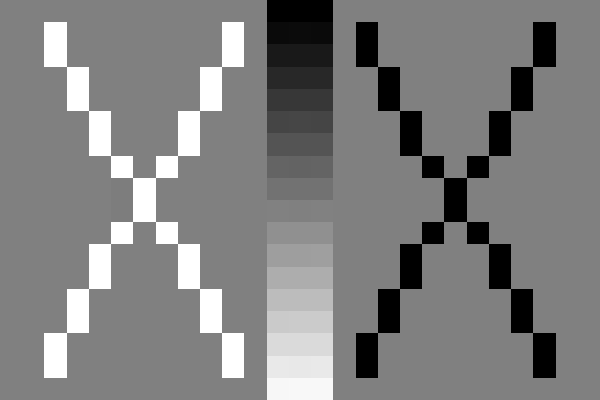
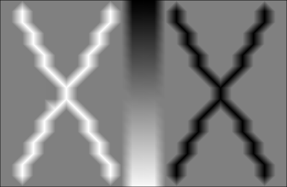
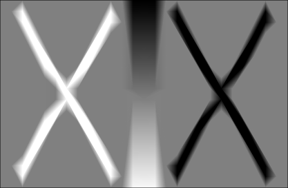
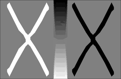
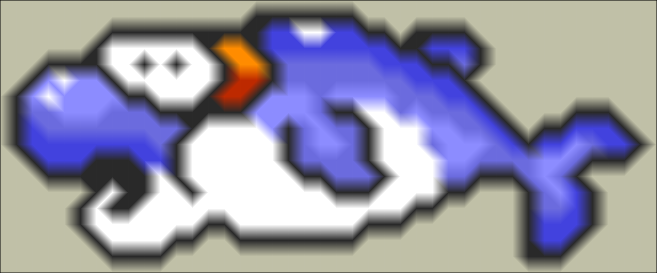
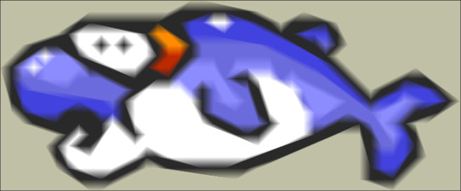
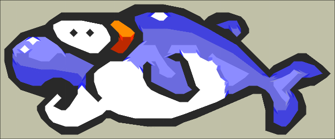
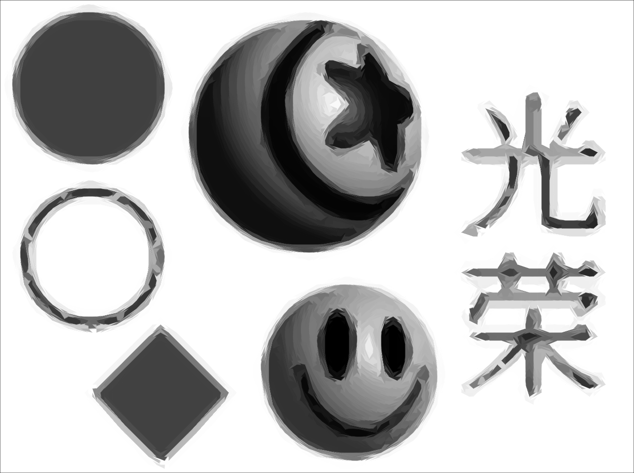
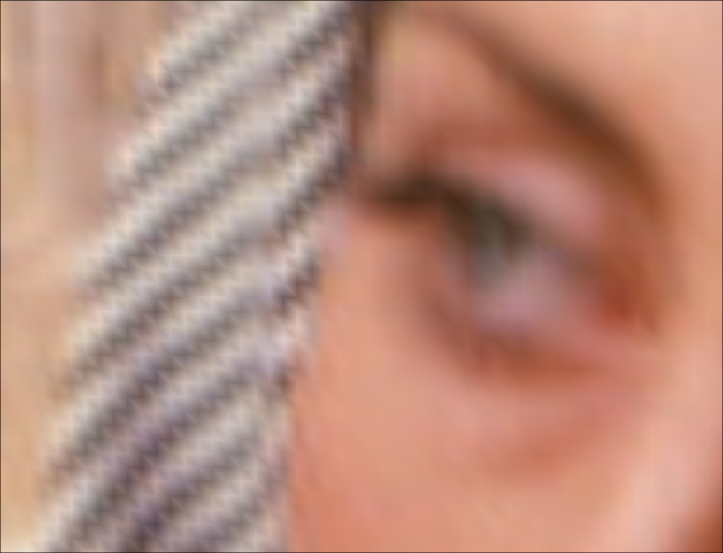
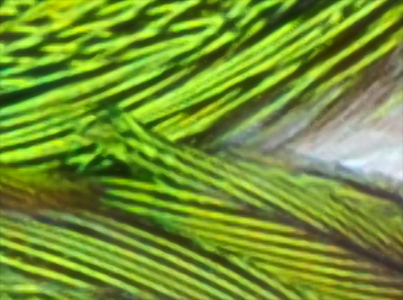
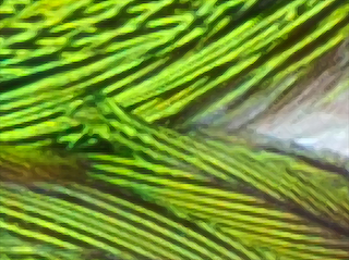
Figure 1: Zoom $\times 16$ of the images in leftmost column: (middle left) displaying the trivial triangulation given by a simple discretization of $\mathrm{TV}$ painted with induced linear gradient over each triangle, (middle right) displaying the triangulation after $\mathrm{GTV}$ optimization painted with induced linear gradient over each triangle, (rightmost) same as before except that triangles are painted with a crisped version of the same gradient.

Figure 1 illustrates the capacity of geometric total variation to capture the direction of image discontinuities. In this simple application, we use the discrete gradient on each triangle to display it with the corresponding linear shaded gradient. Hence we can zoom arbitrarily any image. The results show that, if we stay with the initial triangulation (as does standard discretization of $\mathrm{TV}$), zoomed image are not great. On the contrary, results are considerably improved if we use the optimized triangulation of $\mathrm{GTV}$. Last, we can simply render triangles with a crisped version of this gradient. Results are very nice in case of images with few colors like in pixel art.

3 Contour Regularization

Contours within images are in-between pixels. In some sense they are dual to the structure of the pixels. Since the Geometric Total Variation has structured the relations between pixels, it is natural to define the contours as a kind of dual graph to the optimal triangulation $T^{*}$. We wish also that these contour lines align nicely with discontinuities.

To do so, we introduce a variable $t_{a}$ on each arc whose value is kept in $[0,1]$. If the arc $a$ is the oriented edge $(\mathbf{p},\mathbf{q})$ then the position of the contour crossing this edge will be $\mathbf{x}_{a}=t_{a}\mathbf{p}+(1-t_{a})\mathbf{q}$ (see the upper floating figure).

We denote by $a^{\prime}$ the arc opposite to $a$, i.e. $(\mathbf{q},\mathbf{p})$. The face that is to the left of $a$ is denoted $\mathrm{face}(a)$ while the one to its right is $\mathrm{face}^{\prime}(a)$. We will guarantee that, at the end of each iteration, $\mathbf{x}_{a}=\mathbf{x}_{a^{\prime}}$. We associate to each arc $a=(\mathbf{p},\mathbf{q})$ a dissimilarity weight $w_{a}:=\left\|s(\mathbf{q})-s(\mathbf{p})\right\|_{K}=w_{a^{\prime}}$. We introduce also a point $\mathbf{b}_{f}$ for each face $f$ of $T$, which will lie at a kind of weighted barycenter of the vertices of $f$.

Algorithm 3 regularizes these points and provides a graph of contours that is a meaningful vectorization of the input bitmap image $s$. Note that the function Intersection$(a,\mathbf{y},\mathbf{z})$ returns the parameter $t$ such that $\mathbf{x}_{a}$ lies at the intersection of straight line $(\mathbf{y}\mathbf{z})$ and the arc $a$.

1function RegularizeContours( $s$ : Image, $T$ : Triangulation ) ;

Result: Positions of contour points on arcs and barycenter on faces

2 begin

3       for every face $f=\mathbf{p}\mathbf{q}\mathbf{r}$ of $T$ do  $\mathbf{b}_{f}\leftarrow\frac{1}{3}(\mathbf{p}+\mathbf{q}+\mathbf{r})$;

4       for every arc $a$ of $T$ do

5             if $\neg\textsc{isUpdateable}(a)$ then $t^{(0)}_{a}\leftarrow\frac{1}{2}$;

6             else $t^{(0)}_{a}\leftarrow\textsc{Intersection}(a,\mathbf{b}_{\mathrm{face}(a)},\mathbf{b}_{\mathrm{face}^{\prime}(a)})$;

7            

8      $n\leftarrow 0$;

9       repeat

10             for every face $f$ of $T$ do /* Update barycenters */

11                   $\mathbf{b}_{f}\leftarrow\frac{1}{2}(\mathbf{b}_{f}+\sum_{a\in\partial f}w_{a}\mathbf{x}_{a}/\sum_{a\in\partial f}w_{a})$;

12                  

13            for every arc $a$ of $T$ with $\textsc{isUpdateable}(a)$ do /* Update contours */

14                   $t^{(n)}_{a}\leftarrow\frac{1}{2}(t^{(n)}_{a}+\textsc{Intersection}(a,\mathbf{b}_{\mathrm{face}(a)},\mathbf{b}_{\mathrm{face}^{\prime}(a)})$;

15                  

            /* Average displacements along each edge according to area. */

16             for every arc $a=\mathbf{p}\mathbf{q}$ of $T$ with $\mathbf{p}<\mathbf{q}$ and $\textsc{isUpdateable}(a)$ do

17                   $(\alpha,\alpha^{\prime})\leftarrow\frac{1}{2}(1+1/(6\textsc{Area}(a)),1+1/(6\textsc{Area}(a^{\prime})))$;

18                   $t\leftarrow\frac{1}{2}(\alpha t^{(n)}_{a}+1-\alpha^{\prime}t^{(n)}_{a^{\prime}})$;

19                   $(t^{(n+1)}_{a},t^{(n+1)}_{a^{\prime}})\leftarrow(t,1-t)$ ;

20                  

21            $n\leftarrow n+1$;

22            

23      until $\max_{\text{arc~{}}a\text{~{}of~{}}T}|t^{(n)}_{a}-t^{(n-1)}_{a}|<\epsilon$;

24      return $(\mathbf{x},\mathbf{b})$

25

Algorithm 3 Function RegularizeContours iteratively moves contour points and barycenters such that they align with the edges of the triangulation that delineate image discontinuities.

First it starts with natural positions for $\mathbf{x}$ and $\mathbf{b}$ (resp. middle of arcs and barycenter of faces) at line 3 and line 3. Then it proceeds iteratively until stabilization in the loop at line 3. Each iteration consists of three steps: (i) update barycenters such that they are a convex combination of surrounding contour points weighted by their dissimilarities (line 3), (ii) update contour points such that they lie at the crossing of the arc and the nearby barycenters (line 3), (iii) average the two displacements along each edge according to respective area (line 3), thus guaranteeing that $\mathbf{x}_{a}=\mathbf{x}_{a^{\prime}}$ for every arc. The area $\textsc{Area}(a)$ associated to an arc $a$ is the area of the quadrilateron formed by the tail of $a$, barycenters $\mathbf{b}_{\mathrm{face}(a)}$ and $\mathbf{b}_{\mathrm{face}^{\prime}(a)}$ and $\mathbf{x}_{a}$. Note that the coefficients $\alpha$ and $\alpha^{\prime}$ computed at line 3 have value 1 whenever the area is $\frac{1}{6}$.

	before regularization	after regularization
no $\mathrm{GTV}$
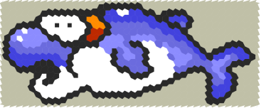
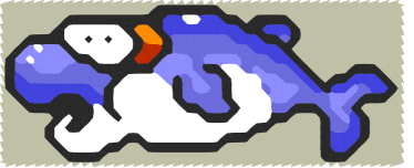
with $\mathrm{GTV}$

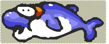
Figure 2: Displays contour mesh: left column before regularization, right column after regularization with Algorithm 3. Top row shows contour meshes when using the initial trivial triangulation. Bottom row shows contour meshes when using the triangulation $T^{*}$ that optimize $\mathrm{GTV}(s)$. Note that boundary triangles are displayed in white.

Since this process is always computing convex combinations of points with convex constraints, it converges quickly to a stable point. In all our experiments, we choose $\epsilon=0.001$ and the process converges in a dozen of iterations. Figure 2 illustrates it. The contour mesh is defined simply as follows: there is one cell per pixel, and for each pixel $\mathbf{p}$, its cell is obtained by connecting the sequence of points $\mathbf{x}_{a_{0}},\mathbf{b}_{\mathrm{face}(a_{0})},\mathbf{x}_{a_{1}},\mathbf{b}_{\mathrm{face}(a_{1})}\ldots$ for every arc $a_{0},a_{1},\ldots$ coming out of $\mathbf{p}$. Each cell of the contour mesh is displayed painted with the color of its pixel. It is clear that the contour mesh is much more meaningful after $\mathrm{GTV}$ optimization, and its further regularization remove some artefacts induced by the discretization. Last but not least, our approach guarantees that sample points always keep their original color.

4 Raster Image Zooming with Smooth Contours

Contour meshes as presented in Section 3 are easily vectorized as polylines. It suffices to gather cells with same pixel color as a regions and extract the common boundaries of these regions. Furthermore, these polylines are easily converted to smooth splines. We will not explore this track in this paper but rather present a raster approach with similar objectives and features.

From the image $s$ with lattice domain $\Omega$, we wish to build a zoomed image $s^{\prime}$ with lattice domain $\Omega^{\prime}$. If the zoom factor is the integer $z$ and $\Omega$ has width $w$ and height $h$, then $\Omega^{\prime}$ has width $z(w-1)+1$ and height $z(h-1)+1$. The canonical injection of $\Omega$ into $\Omega^{\prime}$ is $\iota_{z}:(x,y)\mapsto(zx,zy)$. We use two auxiliary binary images $S$ (for similarity image) and $D$ for (for discontinuity image) with domain $\Omega^{\prime}$. We also define the tangent $\mathbf{T}_{a}$ at an arc $a$ as the normalization of vector $\mathbf{b}_{\mathrm{face}(a)}-\mathbf{b}_{\mathrm{face}^{\prime}(a)}$.

The zoomed image $s^{\prime}$ is constructed as follows:

Similarity set

We set to $1$ the pixels of $S$ that are in $\iota_{z}(\Omega)$. Furthermore, for every arc $a=(\mathbf{p},\mathbf{q})$, if $w_{a}=0$ then the digital straight segment between $\iota_{z}(\mathbf{p})$ and $\iota_{z}(\mathbf{q})$ is also set to $1$. Last, we set the color $s^{\prime}$ at these pixels to their color in $s$.

Discontinuity set

For every face $f$, we count the number $n$ of arcs whose weight is not null. If $n=0$ we simply set $D(\iota_{z}(\mathbf{b}_{f}))=1$. $n=1$ is impossible. If $n=2$, let $a_{1}$ and $a_{2}$ be the two arcs with dissimilarities. We set $D(\mathbf{p})=1$ for every pixel $\mathbf{p}\in\Omega^{\prime}$ that belongs to the digitized Bezier curve of order 3, that links the points $\iota_{z}(\mathbf{x}_{a_{1}})$ to $\iota_{z}(\mathbf{x}_{a_{2}})$, is tangent to $\mathbf{T}_{a_{1}}$ and $\mathbf{T}_{a_{2}}$, and pass through point $\iota_{z}(\frac{1}{2}(\mathbf{b}_{f}+I))$, with $I$ the intersection of the two lines defined by $\mathbf{x}_{a_{i}}$ and tangent $\mathbf{T}_{a_{i}}$, $i=1,2$. If $n=3$, for every arc $a$ of $f$, we set $D(\mathbf{p})=1$ for every pixel $\mathbf{p}\in\Omega^{\prime}$ that belongs to the digitized Bezier curve of order 2 connecting $\iota_{z}(\mathbf{x}_{a})$ to $\iota_{z}(\mathbf{b}_{f})$ and tangent to $\mathbf{T}_{a}$. Last we set the color $s^{\prime}$ at all these pixels by linear interpolation of the colors of pixels surrounding $s$.

Voronoi maps

We then compute the voronoi map $\mathrm{Vor}(S)$ (resp. $\mathrm{Vor}(D)$), which associates to each pixel of $\Omega^{\prime}$ the closest point $\mathbf{p}$ of $\Omega^{\prime}$ such that $S(\mathbf{p})=1$ (resp. such that $D(\mathbf{p})=1$).

Image interpolation

For all pixel $\mathbf{p}$ of $\Omega^{\prime}$ such that $S(\mathbf{p})=0$ and $D(\mathbf{p})=0$, let $\mathbf{q}=\mathrm{Vor}(S)(\mathbf{p})$ and $\mathbf{q}^{\prime}=\mathrm{Vor}(D)(\mathbf{p})$. We compute the distances $d=\|\mathbf{q}-\mathbf{p}\|$ and $d^{\prime}=\|\mathbf{q}^{\prime}-\mathbf{p}\|$. We use an amplification factor $\beta\in[0,1]$: when close to $0$, it tends to make linear shaded gradient while close to $1$, it makes contours very crisp.

$$s^{\prime}(\mathbf{p})=\left\{\begin{array}[]{l}(1-\frac{2d^{\prime}}{d+d^{\prime}})s^{\prime}(\mathbf{q}^{\prime})+\frac{2d^{\prime}}{d+d^{\prime}}(\beta s^{\prime}(\mathbf{q})+(1-\beta)s^{\prime}(\mathbf{q}^{\prime}))\text{~{}when~{}}d^{\prime}\leq d,\\ (1-\frac{2d}{d+d^{\prime}})s^{\prime}(\mathbf{q})+\frac{2d}{d+d^{\prime}}(\beta s^{\prime}(\mathbf{q})+(1-\beta)s^{\prime}(\mathbf{q}^{\prime}))\text{~{}otherwise}.\end{array}\right.$$

In experiments, we always set $\beta=0.75$ which gives good results, especially for image with low quantization. Of course, many other functions can be designed and the crispness could also be parameterized locally, for instance as a function of the $\mathrm{GTV}$ of the triangle.

Antialiasing discontinuities

To get images that are slightly more pleasant to the eye, we perform a last pass where we antialias every pixel $\mathbf{p}$ such that $D(\mathbf{p})=1$. We simply perform a weighted average within a $3\times 3$ window, with pixels in $S$ having weight $4$, pixels in $D$ having weight $0.25$ and other pixels having weight 1.

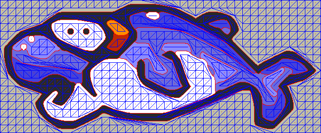
Figure 3: Illustration of raster image zooming with smooth contours. On the left, similarity set is drawn in blue while discontinuity set is drawn in red. The final result is displayed on the right.

Figure 3 illustrates this method of raster image zooming which provides crisp discontinuities that follow Bezier curves. Comparing with Figure 2, image contours are no more polygonal lines but look like smooth curves. Last this method still guarantees that original pixel colors are kept.

5 Experimental Evaluation and Discussion

Our method can both produce vectorized image or make rasterized zoomed images, either from camera pictures or tiny image with low quantization like pixel art images. To measure its performance, several other super-resolution methods have been tested on the set of images given in the first column of Figure 4, with parameters kept constant across all input images. First, we experimented the method based on geometric stencils proposed by Getreuer [6] with default parameters, which is implemented in the online demonstrator [7]. As shown in the second column of the figure, results appear noisy with oscillations near edges, which are well visible on pixel art images (e.g. x-shape or dolphin images). Such defaults are also visible on ara or barbara image near the white area. Another super-resolution method was experimented which uses on a convolutional neural network [22]. Like the previous method, numerous perturbations are also visible both on pixel art images (x-shape or dolphin) but also in homogeneous areas close to strong gradients of ipol-coarsened image. We have tried different parameters but they lead to images with comparable quality. On the contrary, due to its formulation, our method does not produce false contours or false colors, and works indifferently on pixel art images or camera pictures.

	(a) original	(b) Geom. stencil [7]	(c) CNN [22]	(d) Our approach
x-shape
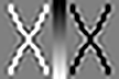
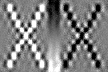
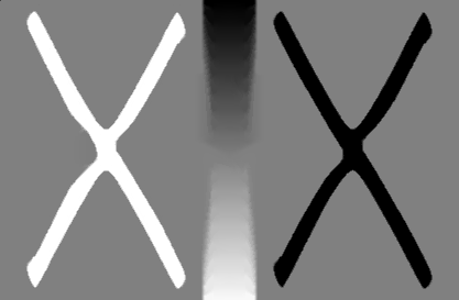
		total time: $8\,ms$	total time: $413\,ms$	total time: $218\,ms$
dolphin
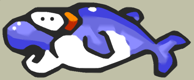
		total time: $11\,ms$	total time: $398\,ms$	total time: $320\,ms$
ipol coarsened
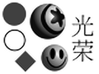
		total time: $63\,ms$	total time:$425\,ms$	total time: 2$032\,ms$
barbara
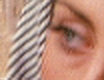
		total time: $28\,ms$	total time: $412\,ms$	total time: 1$029\,ms$
ara
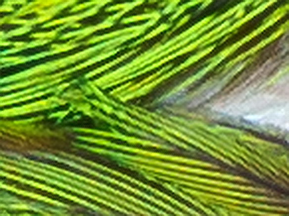
		total time: $202\,ms$	total time: $551\,ms$	total time: $8524\,ms$
The time measures were obtained on a 2.9 GHz Intel Core i7 for (c,d) and on IPOL server for (b).

Figure 4: Comparison of the proposed approach (d) with other methods on Geometric Stencils [7] (b) and based on Convolution Neural Network [22] (c).

Depixelizing [13]	vector magic [10]
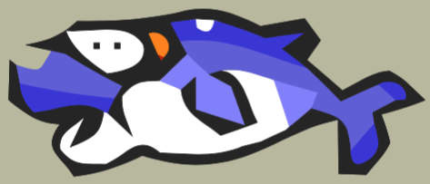
approx. time: $<0.5\,s$	approx. time: $2\,s$
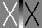
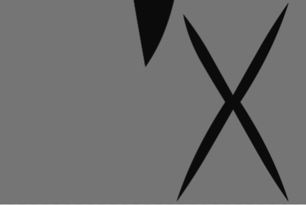
approx. time: $<0.5\,s$	approx. time: $2\,s$

Roussos-Maragos [8]	Potrace [21]
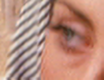
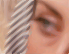
total time : $503\,ms$	approx. time: $5\,s$

$Hq4x$ [23]	$Hq4x(Hq4x)$	$Hq4x$ [23]	$Hq4x(Hq4x)$
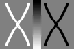
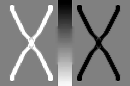
total time : $158\,ms$	total time: $152\,ms$	total time : $142\,ms$	total time: $320\,ms$

Figure 5: Other complementary comparisons on five other approaches. The time measures were obtained on a 2.9 GHz Intel Core i7 for all experiments expect Roussos-Maragos obtained on IPOL server. We use the default parameters expect for Potrace: we select 512 passes with color option.

Other comparisons are presented on Figure 5 in order to give an overview of the behavior of five other methods. The two first methods complement the comparisons on pixel art image with respectively the depixelizing method proposed by Kopf and Lischinski [13] implemented in Inkscape, and a commercial sofware proposed by Vector Magic Inc [10]. Our method captures better the direction of discontinuities of the underlying shape with less contour oscillations (see the border of dolphin or x-shape). Two other methods were tested on barbara image: Roussos and Maragos tensor-driven method [8] and Potrace vectorization software [21]. Again, results appear with oscillations around strong gradients with Roussos-Maragos algorithm, while Potrace software tends to smooth too much the image. Finally we also applied the Hqx magnification filter proposed by Stepin [23] that provides interesting zoom results but presents some artefacts (see for instance the X center of Hq4x) and limited scale factor (i.e. 4). Note that other comparisons can easily be done with the following online demonstrator: https://ipolcore.ipol.im/demo/clientApp/demo.html?id=280 and source code is available on a GitHub repository: https://github.com/kerautret/GTVimageVect.

6 Conclusion

We have presented an original approach to the problem of image vectorization and image super-resolution. It is based on a combinatorial variational model, which introduces geometry into the classical total variation model. We have compared our method both to state-of-the-art vectorization and super-resolution methods and it behaves well both for camera pictures and pixel art images. We have also provided an online demonstrator, which allows users to reproduce results or test our method with new images. In future works, we plan to compare quantitatively our method with state-of-the-art techniques, and also use our approach to train a CNN for zooming into pixel art images.

References

- [1] Partha Bhowmick and Bhargab B. Bhattacharya. Fast Polygonal Approximation of Digital Curves Using Relaxed Straightness Properties. IEEE Transactions on Pattern Analysis and Machine Intelligence, 29(9):1590–1602, 2007.
- [2] Alexander I Bobenko and Boris A Springborn. A discrete laplace–beltrami operator for simplicial surfaces. Discrete & Computational Geometry, 38(4):740–756, 2007.
- [3] Laurent Condat. Discrete total variation: New definition and minimization. SIAM Journal on Imaging Sciences, 10(3):1258–1290, 2017.
- [4] Laurent Demaret, Nira Dyn, and Armin Iske. Image compression by linear splines over adaptive triangulations. Signal Processing, 86(7):1604–1616, 2006.
- [5] Fabien Feschet. Multiscale analysis from 1d parametric geometric decomposition of shapes. In IEEE, editor, ICPR, pages 2102–2105, 2010.
- [6] Pascal Getreuer. Contour Stencils: Total Variation along Curves for Adaptive Image Interpolation. SIAM J. on Imaging Sciences, 4(3):954–979, January 2011.
- [7] Pascal Getreuer. Image Interpolation with Geometric Contour Stencils. Image Processing On Line, 1:98–116, September 2011.
- [8] Pascal Getreuer. Roussos-Maragos Tensor-Driven Diffusion for Image Interpolation. Image Processing On Line, 1:178–186, September 2011.
- [9] Xavier Hilaire and Karl Tombre. Robust and accurate vectorization of line drawings. IEEE TPAMI, 28(6):890–904, 2006.
- [10] Vector Magic Inc. Vector magic, 2010. http://vectormagic.com.
- [11] B. Kerautret, J.-O. Lachaud, and B. Naegel. Curvature based corner detector for discrete, noisy and multi-scale contours. IJSM, 14(2):127–145, December 2008.
- [12] Bertrand Kerautret, Phuc Ngo, Yukiko Kenmochi, and Antoine Vacavant. Greyscale image vectorization from geometric digital contour representations. In DGCI 2017, pages 319–331, 2017.
- [13] Johannes Kopf and Dani Lischinski. Depixelizing Pixel Art. In ACM SIGGRAPH 2011 Papers, pages 99:1–99:8, 2011. Vancouver, British Columbia, Canada.
- [14] Gregory Lecot and Bruno Levy. Ardeco: automatic region detection and conversion. In 17th Eurographics Symposium on Rendering-EGSR’06, pages 349–360, 2006.
- [15] Hairong Liu, Longin Jan Latecki, and Wenyu Liu. A Unified Curvature Definition for Regular, Polygonal, and Digital Planar Curves. Int. J. Comput. Vision, 80(1):104–124, 2008.
- [16] Majed Marji and Pepe Siy. Polygonal representation of digital planar curves through dominant point detection – a nonparametric algorithm. Pattern Recognition, 37(11):2113–2130, 2004.
- [17] Thanh Phuong Nguyen and Isabelle Debled-Rennesson. A discrete geometry approach for dominant point detection. Pattern Recognition, 44(1):32–44, 2011.
- [18] Brian Price and William Barrett. Object-based vectorization for interactive image editing. The Visual Computer, 22(9-11):661–670, September 2006.
- [19] Anastasios Roussos and Petros Maragos. Vector-valued image interpolation by an anisotropic diffusion-projection PDE. In International Conference on Scale Space and Variational Methods in Computer Vision, pages 104–115. Springer, 2007.
- [20] Leonid I. Rudin, Stanley Osher, and Emad Fatemi. Nonlinear total variation based noise removal algorithms. 1992.
- [21] Peter Selinger. Potrace: http://potrace.sourceforge.net, 2001-2017.
- [22] Wenzhe Shi, Jose Caballero, Ferenc Huszar, Johannes Totz, Andrew P. Aitken, Rob Bishop, Daniel Rueckert, and Zehan Wang. Real-Time Single Image and Video Super-Resolution Using an Efficient Sub-Pixel Convolutional Neural Network. In CVPR, pages 1874–1883, Las Vegas, NV, USA, June 2016. IEEE.
- [23] M. Stepin. Hqx magnification filter, 2003. http://web.archive.org/web/20070717064839/www.hiend3d.com/hq4x.html.
- [24] Jian Sun, Lin Liang, Fang Wen, and Heung-Yeung Shum. Image vectorization using optimized gradient meshes. In Trans. on Graphics, volume 26, page 11. ACM, 2007.
- [25] S. Swaminarayan and L. Prasad. Rapid Automated Polygonal Image Decomposition. In 35th Workshop AIPR’06, pages 28–28, October 2006.
- [26] Tian Xia, Binbin Liao, and Yizhou Yu. Patch-based image vectorization with automatic curvilinear feature alignment. In Trans. on Graphics, volume 28, page 115. ACM, 2009.