Kyrix-S: Authoring Scalable Scatterplot Visualizations
of Big Data

Abstract

Static scatterplots often suffer from the overdraw problem on big datasets where object overlap causes undesirable visual clutter. The use of zooming in scatterplots can help alleviate this problem. With multiple zoom levels, more screen real estate is available, allowing objects to be placed in a less crowded way. We call this type of visualization scalable scatterplot visualizations, or SSV for short. Despite the potential of SSVs, existing systems and toolkits fall short in supporting the authoring of SSVs due to three limitations. First, many systems have limited scalability, assuming that data fits in the memory of one computer. Second, too much developer work, e.g., using custom code to generate mark layouts or render objects, is required. Third, many systems focus on only a small subset of the SSV design space (e.g. supporting a specific type of visual marks). To address these limitations, we have developed Kyrix-S, a system for easy authoring of SSVs at scale. Kyrix-S derives a declarative grammar that enables specification of a variety of SSVs in a few tens of lines of code, based on an existing survey of scatterplot tasks and designs. The declarative grammar is supported by a distributed layout algorithm which automatically places visual marks onto zoom levels. We store data in a multi-node database and use multi-node spatial indexes to achieve interactive browsing of large SSVs. Extensive experiments show that 1) Kyrix-S enables interactive browsing of SSVs of billions of objects, with response times under 500ms and 2) Kyrix-S achieves 4X-9X reduction in specification compared to a state-of-the-art authoring system.

K.6.1Management of Computing and Information SystemsProject and People ManagementLife Cycle; K.7.mThe Computing ProfessionMiscellaneousEthics A scalable scatterplot visualization created by Kyrix-S and its Kyrix-S specifications. One billion comments made by users on Reddit.com from Jan 2013 to Feb 2015 are visualized on 15 zoom levels. On every level, $X$ and $Y$ axes are respectively the posting time and length of the comments. Each circle represents a cluster of comments. The number inside each circle is the size of the cluster and also encodes the radius of the circle. Using pan or zoom, the user can get either an overview (left) or inspect an area of interest (middle). One can hover over a circle to see three highest-scored comments in the cluster, as well as a bounding box showing the boundary of the cluster.

1 Introduction

Scatterplots are an important type of visualization used extensively in data science and visual analytic systems. Objects in a dataset are visualized on a 2D Cartesian plane, with the dimensions being two quantitative attributes from the objects. Each object can be represented as a point, polygon or other mark. Aggregation-based marks (e.g. pie chart, heatmap) can also be used to represent groups of objects. The user of a scatterplot can perform a variety of tasks to provide insights into the underlying data, such as discovering global trends, inspecting individual objects or characterizing distributions[46].

Despite the usefulness of static scatterplots, they suffer from significant overdraw problem on big datasets[43, 37]. Here, we focus on scatterplots with millions to billions of objects, where significant overlap of marks is unavoidable, making the visualization ineffective. To address this issue in scatterplots, there has been substantial research[24, 25, 36, 33] on devising aggregation-based scatterplots using visual aggregates such as contours or hexagon bins. While avoiding visual clutter, these approaches do not support inspecting individual objects, which is a fundamental scatterplot task[46]. Prior works also used transparency[22, 30], animation[12] and displacements of objects[51, 28, 50] to ease the overdraw problem. However, due to limited screen resolution, these methods have scalability limits.

On the other hand, the use of zooming in scatterplots has the potential to effectively mitigate visual clutter. By expanding the 2D Cartesian plane into a series of zoom levels with different scales, more screen resolution becomes available, allowing for object layouts that avoid occlusion and excessive density. Inspecting large amounts of objects thus becomes feasible. Aggregation-based marks such as circles or heatmaps can still be used to visualize groups of objects. Figure Kyrix-S: Authoring Scalable Scatterplot Visualizations of Big Data shows such a visualization created by the system we introduce in this paper, which shows one billion comments made by users on Reddit.com, where $X$ is the posting time and $Y$ is the number of characters in the comments. Additional examples are in Figure 1. For simplicity, we term such visualizations scalable scatterplot visualizations, or SSV.

There has been significant work on building systems/toolkits to aid the creation of SSVs (e.g.[49, 5, 23, 15]). Specifically, prior systems can be classified into two categories: general pan/zoom systems and specialized SSV systems. General pan/zoom systems are typically expressive, supporting not only SSVs, but also pan/zoom visualizations of other types of data (e.g. hierarchical and temporal data) or that connect multiple 2D semantic spaces. Specialized SSV systems (e.g. [23, 11]), on the other hand, generally have a narrow focus on SSVs.

While these systems have been shown to be effective, they can suffer from some drawbacks that limit their ability to support general SSV authoring at scale. In particular, limited scalability is a common drawback of both types of systems. As often as not, implementations assume all objects reside in the main memory of a computer[11, 37, 32, 23, 33, 38, 5, 45].

General pan/zoom systems, while being flexible, generally incur too much developer work due to their low-level nature. When authoring an SSV, the developer needs to manually generate the layout of visual marks on zoom levels. In very large datasets, there will be many levels (e.g. Google Maps has 20). Individually specifying the layout of a set of levels is tedious and error-prone. In particular, big or skewed data can make it challenging for the developer to specify a layout that avoids occlusion and excessive density in the visualization.

Another drawback of specialized SSV systems is low flexibility. Oftentimes systems are hardcoded for specific scenarios (e.g., supporting specific types of visual marks such as heatmaps[43, 33] or points[15, 11], enforcing a density budget but not removing overlap, etc.) and are not extensible to general use cases. The developer cannot make free design choices when using these systems, and is forced to constantly switch tools for different application requirements.

In this paper, we describe Kyrix-S , a system for SSV authoring at scale which addresses all issues of existing systems. To enable rapid authoring, we present a high-level declarative grammar for SSVs. We abstract away low-level details such as rendering of visual marks so that the developer can author a complex SSV in a few tens of lines of JSON. We show that compared to a state-of-the-art system, this is 4X–9X reduction in specification on several examples. In addition, we build a gallery of SSVs to show that our grammar is expressive and that the developer can easily extend it to add his/her own visual marks.

This grammar for SSVs is supported by an algorithm that automatically chooses the layout of visual marks on all zoom levels, thereby freeing the developer from writing custom code. We store objects in a multi-node parallel database using multi-node spatial indexing. As we show in Section 8, this allows us to respond to any pan/zoom action in under 500ms on datasets with billions of objects.

To summarize, we make the following contributions:

• An integrated system called Kyrix-S for declarative authoring and rendering of SSVs at scale.

• A concise and expressive declarative grammar for describing SSVs (Section 4).

• A framework for offline database indexing and online serving that enables interactive browsing of large SSVs (Sections 5 and 6).

2 Related Works

2.1 General Pan/zoom Systems

A number of systems have been developed to aid the creation of general pan/zoom visualizations[5, 6, 45, 49]. These systems are expressive and capable of producing not only SSVs, but also pan/zoom visualizations of other types of data (e.g. hierarchical, temporal, etc) or with multiple semantic spaces connected by semantic zooms[45]. However, as mentioned in the introduction, these systems fall short in supporting SSVs due to limited scalability and too much developer work.

Kyrix[49] is a general pan/zoom system we have developed. Here, we summarize the novel aspects of Kyrix-S compared to Kyrix and similar systems (e.g., ForeCache [4], Nanocubes [33], imMens [36]):

• Kyrix-S provides a high-level grammar for SSVs, which enables much shorter specification than what Kyrix’s grammar requires for the same SSV (see Section 8.2 for an empirical comparison);

• Kyrix-S implements a layout generator which frees the developer from deciding the layout of objects on zoom levels. Kyrix does not assist the developer in choosing an object layout, which makes authoring SSVs using Kyrix fairly challenging;

• Kyrix-S is integrated with a distributed database which scales to billions of objects. In contrast, Kyrix only works with a single-node database which cannot scale to billions of objects.

Note that Kyrix-S has a narrow focus on SSVs and is not intended to completely replace general pan/zoom systems. As we will discuss more in Section 7, we implement Kyrix-S as an extension to Kyrix.

2.2 Specialized SSV Systems

There has been considerable effort made to develop specialized SSV systems, which mainly suffer from two limitations: low flexibility and limited scalability.

Many systems focus on a small subset of the SSV design space, and are not designed/coded to be easily extensible. For example, many focus on specific visual marks such as small-sized dots (e.g.[15, 11, 27]), heatmaps (e.g.[43, 33, 41, 38, 34]), text[44], aggregation-based glyphs[32, 7] and contours[37]. Some works maintain a visual density budget[15, 43, 23], while some focus on overlap removal[7, 11, 17]. In contrast to these systems, Kyrix-S aims at a much larger design space. We provide a diverse library of visualization templates that are suitable for a variety of scatterplot tasks. For high extensibility, Kyrix-S’s declarative grammar is designed with extensible components for authoring custom visual marks.

In addition to the limited focus, most specialized SSV systems cannot scale to large datasets with billions of objects due to an in-memory assumption[1, 16, 23, 37, 11, 31, 19, 40]. We are only aware of the work by Perrot et al.[43] which renders large heatmaps using a distributed computing framework. However, that work only focuses on heatmaps.

Specialized SSV systems generally come with a layout generation module which computes the layout of visual marks on each zoom level. The design of Kyrix-S’s layout generation is inspired by many of them and bears similarities in some aspects. For example, favoring placements of important objects on top zoom levels is adopted by many works[23, 44, 15]. The idea of enforcing a minimum distance between visual marks comes from blue-noise sampling strategies[43, 11, 23].

However, the key differentiating factor of Kyrix-S comes from its more stringent requirements on scalability and the design space. These requirements (see Section 3) pose new algorithmic challenges. For instance, Sarma et al.[15] uses an integer programming solution without considering overlaps of objects. To enable overlap removal, one needs to add $O(n^{2})$ pairwise non-overlap constraints into the integer program, making it hard to solve in reasonable time. As another example, Guo et al.[23] and Chen et al.[11] do not support visual marks that show a group of objects with useful aggregated information. This requires a bottom-up aggregation process which breaks their top-down algorithmic flow. In order to scale to billions of objects, Kyrix-S cannot rely on existing algorithms and instead needs to compute visual mark layouts in parallel using a distributed algorithm as described in Section 6.

2.3 Static Scatterplot Designs

Alleviating the overdraw problem of static scatterplot visualizations has been a popular research topic for a long time. Many methods have been proposed, including binned aggregation[39, 36, 25], appearance optimization[22, 30, 12], data jittering[51, 28, 50] and sampling[18, 13]. We refer interested readers to existing surveys on scatterplot tasks and designs[46], binned aggregation[24] and visual clutter reduction[20, 21]. Kyrix-S’s design follows many guidelines in these works, which we elaborate in Section 3.

2.4 Declarative Visualization Grammars

Numerous declarative grammars have been proposed for authoring visualizations at different levels of abstractions. The first of these is Wilkinson’s grammar of graphics (GoG)[53], which forms the basis of subsequent works. For example, ggplot2[52] is the direct implementation of GoG in R and is widely used. D3[10] and Protovis[9] are low-level libraries that provide useful primitives for authoring basic visualizations. Vega is the first grammar that concerns specifications of interactions. Built on top of Vega, Vega-lite[47] offers a more succinct grammar for authoring interactive graphics. Recently, more specialized grammars have emerged for density maps[25], unit visualizations[42], and pan/zoom visualizations[49].

Despite the diversity of this literature, not many grammars support SSVs well. Some low-level grammars such as D3[10], Vega[48] and Kyrix[49] can express SSVs, but the specification is often verbose due to their low-level and general-purpose nature. Kyrix-S, on the contrary, uses a high-level grammar that abstracts away unimportant low-level details. For example, switching mark representations can be simply done by changing a renderer type parameter (e.g. from “circle” to “heatmap”) without writing a renderer. Furthermore, different from aforementioned grammars, Kyrix-S’s grammar allows specifications of multiple zoom levels altogether with convenient components for specifying sampling/aggregation semantics.

3 Design Goals

Limitations of prior art, existing guidelines and our experience with SSV users drive the design of Kyrix-S. Here, we present a few goals we set out to achieve.

G1. Rapid authoring. Our declarative grammar should enable specification of SSVs in a few tens of lines of code. This goal is inspired by the design rationale of several high-level declarative languages (e.g. Vega-lite[47] and Atom[42]), and driven by the limitations we see in using Kyrix[49] to author SSVs.

G2. Visual expressivity. Kyrix-S should enable the exploration of a broad SSV design space and not limit itself to specific visual representations. Moreover, it is crucial to allow inspection of individual objects in addition to showing aggregation information. As outlined by Sarikaya et al. [46], there are four common object-centric scatterplot tasks: identify object, locate object, verify object and object comparison. A recent study[31] also highlights the importance of browsing objects in multi-scale visualizations.

G3. Usable SSVs. The SSVs authored with Kyrix-S should be usable, e.g. free of visual clutter, using simple visual aggregates, etc. We identify usability guidance from a range of surveys and SSV systems (e.g.[21, 23, 15]), which we formally describe in Section 6.

G4. Scalability. Kyrix-S should be able to handle large datasets with billions of objects and potentially skewed spatial distribution. This goal has the following two subgoals:

• G4-a. Scalable offline indexing. Offline indexing should finish in reasonable time on big data, and scale well as the data size grows.

• G4-b. Interactive online serving. The end-to-end response time to any user interaction (pan or zoom) should be under 500ms, an empirical upper bound that ensures fluid interactions[35].

In the rest of the paper, we justify the design choices we make by referencing the above goals when appropriate.

4 Declarative Grammar

In this section, we present Kyrix-S’s declarative grammar. We start with showing a gallery of example SSVs authored with Kyrix-S (Section 4.1), which we then use to illustrate the design of the grammar in Section 4.2.

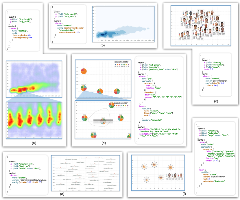
Figure 1: A gallery of SSVs authored with Kyrix-S and their specifications. (a): a heatmap of 178.3 million taxi trips in Chicago since 2013, $X$: trip length (seconds), $Y$: trip total (dollars); (b): the same dataset/axes as (a) in contour plots; (c): an SSV of 18,207 soccer players in the video game FIFA19, $X$: shooting rating, $Y$: defense rating, $Z$: wage (i.e. highly-paid players appear on top zoom levels); (d): a pie-based SSV of 17.3 million liquor purchases by retailers in Iowa, $X$: unit price (dollars), $Y$: quantity (# of bottles), $Z$: purchase date; (e): a text visualization of the dataset of one billion Reddit comments in Figure Kyrix-S: Authoring Scalable Scatterplot Visualizations of Big Data with the same axes; (f): the same dataset/axes as (c) in a radar-chart.

4.1 Example SSVs

Figure 1 shows a gallery of SSVs and their specifications.

Taxi. In Figure 1a, a multi-scale heatmap shows 178.5M taxi trips in Chicago since 2013, where $X$ is trip length (in seconds) and $Y$ is trip total (in dollars). In the overview (upper), the long thin “heat” region suggests that most trips have a similar total-length ratio. In a zoomed-in view (lower), we see vertical “heat” regions around entire minutes. In fact, more than 70% of the trips have a length of entire minutes, indicating the possible prevalent use of minute-precision timers. Figure 1b is the same representation of this dataset in contour lines.

FIFA. The SSV in Figure 1c visualizes 18,207 soccer players in the video game FIFA 19. $X$ and $Y$ are respectively the shooting and defensive rating of players. Players with the highest wages are shown at top levels. Lesser-paid players are revealed as one zooms in. Figure 1f is a radar-based SSV with the same $X$ and $Y$. Each radar chart shows the averages of eight ratings (e.g. passing, power) of a cluster of players. When hovering over a radar, three players from that cluster with the highest wages are shown.

Liquor. Figure 1d is an SSV of 17.3M liquor purchases by retailers in Iowa since 2012. $X$ and $Y$ axes are the unit price (dollars) and quantity (# of bottles) of the purchases. Each pie shows a cluster of purchases grouped by day of the week. One can hover over a pie to see a tabular visualization of the three most recent purchases, as well as a convex hull showing the boundary of the cluster.

Reddit. Figure 1e is another representation of the one-billion Reddit comments dataset. Different from Figure Kyrix-S: Authoring Scalable Scatterplot Visualizations of Big Data, comments are directly visualized as non-overlapping texts. The number above each comment represents how many comments are nearby, giving the user an understanding of the data distribution hidden underneath.

4.2 Grammar Design

$$\langle\textrm{\mbox{SSV}}\rangle ::= \langle\textrm{Marks}\rangle\langle\textrm{Layout}\rangle\langle\textrm{Data}\rangle[\textrm{Config}]$$

; marks

$$\langle\textrm{Marks}\rangle ::= \langle\textrm{Cluster}\rangle[\textrm{Hover}]$$ (2)

$$\langle\textrm{Cluster}\rangle ::= \langle\textrm{Mode}\rangle\langle\textrm{Aggregate}\rangle[\textrm{Config}]$$ (3)

$$\langle\textrm{Hover}\rangle ::= \langle\textrm{Ranklist}\rangle\langle\textrm{Boundary}\rangle[\textrm{Config}]$$ (4)

$$\langle\textrm{Mode}\rangle ::= \textit{Circle}\;\mid\;{}\textit{Contour}\;\mid\;{}\textit{heatmap}\;\mid\;{}$$ (5)

$$\textit{Radar}\;\mid\;{}\textit{Pie}\;\mid\;{}\langle\textrm{Custom}\rangle$$

$$\langle\textrm{Aggregate}\rangle ::= \langle\textrm{Dimension}\rangle*\langle\textrm{Measure}\rangle+$$ (6)

$$\langle\textrm{Ranklist}\rangle ::= \langle\textrm{Topk}\rangle(\textit{Tabular}\;\mid\;{}\langle\textrm{Custom}\rangle)$$ (7)

$$\langle\textrm{Boundary}\rangle ::= \textit{Convex Hull}\;\mid\;{}\textit{BBox}$$ (8)

$$\langle\textrm{Custom}\rangle ::=$$ Custom JS mark renderer (9)

$$\langle\textrm{Dimension}\rangle ::= \langle\textrm{Field}\rangle[\textrm{Domain}]$$ (10)

$$\langle\textrm{Measure}\rangle ::= \langle\textrm{Field}\rangle\langle\textrm{Function}\rangle[\textrm{Extent}]$$ (11)

$$\langle\textrm{Topk}\rangle ::=$$ A positive integer (12)

$$\langle\textrm{Domain}\rangle ::=$$ A list of string values (13)

$$\langle\textrm{Function}\rangle ::= \textit{Count}\;\mid\;{}\textit{Sum}\;\mid\;{}\textit{Avg}\;\mid\;{}\textit{Min}\;\mid\;{}$$

$$\textit{Max}\;\mid\;{}\textit{Sqrsum}$$

; layout

$$\langle\textrm{Layout}\rangle ::= \langle\textrm{X}\rangle\langle\textrm{Y}\rangle\langle\textrm{Z}\rangle[\textrm{Theta}]$$ (15)

$$\langle\textrm{X}\rangle ::= \langle\textrm{Field}\rangle[\textrm{Extent}]$$ (16)

$$\langle\textrm{Y}\rangle ::= \langle\textrm{Field}\rangle[\textrm{Extent}]$$ (17)

$$\langle\textrm{Z}\rangle ::= \langle\textrm{Field}\rangle\langle\textrm{Order}\rangle$$ (18)

$$\langle\textrm{Theta}\rangle ::=$$ A number between 0 and 1 (19)

$$\langle\textrm{Field}\rangle ::=$$ A database column name (20)

$$\langle\textrm{Extent}\rangle ::=$$ A pair of float numbers (21)

$$\langle\textrm{Order}\rangle ::= \textit{Ascending}\;\mid\;{}\textit{Descending}$$

; data

$$\langle\textrm{Data}\rangle ::=$$ a database query

; config

$$\langle\textrm{Config}\rangle ::=$$ Key value pairs (24)

Figure 2: Kyrix-S’s declarative grammar in the BNF notation. Inside $\langle\rangle$ or [] is a component. Every rule (1-24) defines what the left-hand side component is composed of. On the right hand side of a rule, $|$ means OR, * means zero or more, + means one or more and [] means that a component is optional.

The primary goal of Kyrix-S’s declarative grammar is to help the developer quickly navigate a large SSV design space (G1 and G2). The high-level design of the grammar closely follows a survey of scatterplots designs and tasks by Sarikaya et al.[46], which outlined four common design variables of scatterplot visualizations: point encoding (i.e. visual representation of one object), point grouping (i.e. visual representation of a group of objects), point position (e.g. subsampling, zooming) and graph amenities (e.g. axes, annotations). These design variables map to the highest-level components in Kyrix-S’s grammar, i.e., Marks, Layout, Data and Config, as illustrated in Figure 2 using the BNF notation[29]. We elaborate the design of them in the following.

4.2.1 Marks: Templates + Extensible Components

The Marks component (Rules 2-14) defines the visual representation of one or more objects, and covers both point encoding and point grouping in [46]. Visual marks of a single or a cluster of objects span a huge space of possible visualizations. To keep our grammar high-level (G1), we adopt a templates+extensible components methodology, where we provide a diverse library of template mark designs, and offer extensible components for authoring custom marks.

We divide the Marks component into two subcomponents: Cluster (Rule 3) and Hover (Rule 4).

Cluster: cluster marks are static marks rendering one or a group of objects. Currently, Kyrix-S has five built-in Cluster marks including Circle (Figure Kyrix-S: Authoring Scalable Scatterplot Visualizations of Big Data), Contour (Figure 1b), Heatmap (Figure 1a), Radar (Figure 1f) and Pie (Figure 1d). The developer can choose one of these marks by specifying just a name (G1). These built-in Cluster marks are carefully chosen to cover a range of aggregate-level SSV tasks[46]. For example, heatmaps and contour plots enable the user to characterize distribution and identify correlation between the two axes. The user can perform numerosity comparison and identify anomalies with circle-based SSVs. Radar-based and pie-based SSVs allow for exploring object properties within a neighborhood. For fast authoring, Kyrix-S sets reasonable default values for many parameters (G1), e.g., inner/outer radius of a pie and bandwidth of heatmaps. The developer can also customize (G2-b) using a Config component (Rules 3 and 24).

With the Custom component (Rules 5 and 9), the developer can specify custom visual marks easily. For example, player profiles in Figure 1c are specified as a custom visual mark. Kyrix-S currently supports arbitrary Javascript-based renderers (e.g. D3[10] or Vega-lite-js[3]). For increased expressivity, a custom mark renderer is passed all useful information about a cluster of objects, including aggregation information in both Aggregate and Hover. As an example, the custom renderer in Figure 1e displays both an example comment and the size of the cluster. More importantly, Custom also facilitates rapid future extension of Kyrix-S, allowing easy addition of built-in mark types.

The Aggregate component (Rule 6) specifies details of aggregations statistics shown by a Cluster mark, and is composed of Dimensions (Rule 10) and Measures (Rule 11). A Dimension is a categorical field of the objects indicating how objects are grouped (e.g. by day of the week in Figure 1d). A Measure defines an aggregation statistic (e.g. average of a rating in Figure 1f). Currently Kyrix-S supports six aggregation functions: count, average, min, max, sum and square sum (Rule 14).

Hover: Hover marks add more expressivity into the grammar by showing additional marks when the user hovers over a Cluster mark. For example, in Figure Kyrix-S: Authoring Scalable Scatterplot Visualizations of Big Data three example comments are shown upon hovering a circle. The motivation for adding this component is two-fold.

First, as outlined in G2, we want to enable tasks that require inspection of individual objects in addition to showing visual aggregates with Cluster marks. To this end, we design a Ranklist component which visualizes objects with top-k importance (Rule 7). The importance of objects is defined in the layout component as a field from the objects. We offer a default tabular visualization template (e.g. Figure 1d), and allow custom marks via Custom (e.g. player profiles in Figure 1f).

Secondly, multi-scale visualizations often suffer from the “desert fog” problem[26], where the user is lost in the multi-scale space and not sure what is hidden underneath the current zoom level. Boundary is designed to aid the user in navigating (G3) by showing the boundaries of a cluster of objects (Rule 8), using either the convex hull (Figure 1d) or the bounding box (Figure Kyrix-S: Authoring Scalable Scatterplot Visualizations of Big Data). By hinting that there is more to see by zooming in, more interpretability is added to the visualization.

4.2.2 Layout: Configuring All Zoom Levels at Once

The Layout component (Rules 15-22) controls the placement of visual marks on zoom levels, which corresponds to the point position design variable in [46]. We aim to assist the developer in specifying the layout for all zoom levels together rather than independently, motivated by the limitation of general pan/zoom systems[49, 6, 5] that mark placements are manually configured for every zoom level.

$X$ and $Y$ (Rules 16 and 17) define the two spatial dimensions. The only specifications required are two raw data columns that map to the two dimensions (e.g. trip length and total in Figures 1a and 1b). An optional Extent component (Rule 21) can be used to indicate the visible range of raw data values on the top zoom level.

The $Z$ component (Rule 18) controls how visual marks are distributed across zoom levels. Drawn from prior works[15, 23, 44], we use a usability heuristic that makes objects with higher importance more visible on top zoom levels. The importance is defined by a field of the objects. For example, in Figure 1e, highest-scored comments are displayed on top zoom levels.

Optionally, Theta is a number between 0 and 1 indicating the amount of overlap allowed between Cluster marks (Rule 19), with 0 being arbitrary overlap is allowed and 1 being overlap is not allowed. For instance, Theta is 0.5 in Figure 1c, making the player profiles overlap to a certain degree.

The above layout-related parameters serve as inputs to the layout generator, which we detail in Section 6.

4.2.3 Data and Config

We assume that the raw spatial data exists in the database, and can be specified as a SQL query (Rule 23). The highest-level Config component corresponds to the design variable graph amenities in[46]. The developer can use it to specify global rendering parameters such as the size of the top zoom level, number of zoom levels, as well as annotations such as axes, grid lines and legends.

5 Optimization Framework

Figure 3: Kyrix-S optimization framework.

Figure 3 illustrates the optimization framework adopted by Kyrix-S to scale to large datasets(G4). There are two main phases: offline indexing and online serving. Specifically, given an SSV specification, the layout generator computes offline the placement of visual marks on zoom levels using several usability considerations (G3), e.g., bounded visual density, free of clutter, etc. Along the way, useful aggregation information (e.g. statistics and cluster boundaries) is also collected. The computed layout information is stored in a multi-node database with multi-node spatial indexes. Online, the data fetcher communicates with the frontend and fetches data in user’s viewport from the multi-node database with sub-500ms response times (G4-b). In the next section, we describe these two components in greater detail.

6 Layout Generation and Data Fetching

Here, we first describe how we model the layout generation problem (Section 6.1). We then describe a single-node layout algorithm (Section 6.2), which is the basis of a distributed algorithm detailed in Section 6.3. Lastly, Section 6.4 describes the design of the data fetcher.

6.1 Layout Generation: Problem Definition

We assume that there is a discrete set of zoom levels numbered 1, 2, 3$\ldots$ from top to bottom with a constant zoom factor between adjacent levels (e.g. 2 as in many web maps). The layout generation problem concerns how to, in a scalable manner, place visual marks onto these zoom levels in a general way that works for any SSV that Kyrix-S’s declarative grammar can express (G2).

To aid the formulation of the layout generation problem, we collect a set of existing layout-related usability considerations from prior SSV systems and surveys[23, 7, 11, 15, 21, 32], and list them as subgoals of G3: Usable SSVs.

G3-a. Non/partial overlap. Cluster visual marks (Rule 3) should not overlap or only overlap to a certain degree (if specified by Theta in Rule 19). For simplicity, we assume that Cluster marks have a fixed-size bounding box, which is either decided by Kyrix-S or specified by the developer (see Figure 1e for an example). We then only check the overlap of bounding boxes.

G3-b. Bounded visual density. Mark density in any viewing region should not exceed an upper bound. Excessive density stresses the user and slows down both the client and the server. Kyrix-S sets a default upper bound $K$ on how many marks should exist in any viewport-sized region based on empirical estimates of the processing capability of the database and the frontend. We should also avoid very low visual density, which often leads to too many zoom levels and thus increased navigation complexity. We therefore try to maximize spatial fullness without violating the overlap constraint and the density upper bound.

G3-c. Zoom consistency. If one object is visible on zoom level $i$, either through a custom Cluster mark or a Ranklist mark (Rule 7), it should stay visible on all levels $j>i$. This principle is adopted by many SSV systems that support inspection of individual objects (e.g. [15, 11, 23]). The rationale is to aid object-centric tasks where keeping track of locations of objects is important.

G3-d. Data abstraction quality. Data abstraction characterized by visual marks should be interpretable and not misinform the user. For Cluster marks, it is important to reduce within-cluster variation[14, 54, 21], which can be characterized by average distance of objects to the visual mark that represent them[14]. We also adopt an importance policy, where objects with higher importance (Rule 18) should be more likely to be visible on top zoom levels. This is a commonly adopted principle to help the user see representative objects early on[23, 15].

Discussion. Despite that subgoals G3-a$\sim$d are all from existing works, we are not aware of any prior system that addresses all of them. As mentioned in Section 2, a key distinction of Kyrix-S’s layout generation lies in the more stringent requirements of scalability and the design space. Due to this broad focus, finding an “optimal layout” with the objectives and constraints in G3-a$\sim$d is hard. In fact, a prior work[15] proves that with only a subset of G3-a$\sim$d, finding the optimal layout is NP-hard (for an objective function they define). Therefore, we do not attempt to define a formal constraint solving problem. Instead we keep our goals qualitative and look for heuristic solutions.

6.2 A Single-node Layout Algorithm

Here, we describe a single-node layout algorithm which assumes that data fits in the memory of one computer.

We assume that the $X$/$Y$ placement of a Cluster mark comes from an object it represents. Alternatively, one could consider inexact placement of the marks (e.g. “median location” or binned aggregation), which we leave as our future work. Additionally, we assume that the $X$/$Y$ placement of a Hover mark is the same as the corresponding Cluster mark. So in the rest of Section 6, any mention of mark refers to a Cluster mark if not explicitly stated.

We make two important algorithmic choices. First, we enforce a minimum distance between marks in order to cope with the overlap and density constraints (G3-a and G3-b). Second, we use a hierarchical clustering algorithm to ensure zoom consistency (G3-c) and data abstraction quality (G3-d).

Figure 4: Marks $P$ and $Q$ with an $ncd$ of $\theta$. Inner boxes (dashed) are the bounding boxes of the marks. Outer boxes (solid) are bounding boxes scaled by a factor of $\theta$. Scaled boxes do not overlap and touch on one side. In general, for any two marks that have $ncd$ greater than $\theta$, their bounding boxes do not overlap after being scaled by a factor of $\theta$.

Enforcing a minimum distance between marks. For overlap and density constraints, we make use of the normalized chessboard distance ($ncd$) between two marks $P$ and $Q$:

$$ncd(P,Q)=\max(\frac{|P_{x}-Q_{x}|}{W_{B}},\frac{|P_{y}-Q_{y}|}{H_{B}})$$

where $P_{x}$($P_{y}$) is the $x$($y$) coordinate of the centroid of $P$ in the pixel space and $W_{B}$($H_{B}$) is the width (height) of the bounding box of a mark (note that bounding boxes of marks are of the same size).

$ncd$ helps us reason about non/partial overlap constraints. If $ncd(P,Q)\geq 1$, $P$ and $Q$ do not overlap because they are at least one bounding box width/height away on $X$ or $Y$. Even if $ncd$ is smaller than one, the degree of overlap is bounded. For example, if $ncd(P,Q)=0.5$, the centroids of $P$ and $Q$ remain visible despite the potential overlap.

To this end, we set a lower bound $\theta$ on the $ncd$ between any two visual marks, which is specified through the Theta component (e.g. Figure 1c) or built-in with Cluster marks.

We also use $\theta$ to enforce the visual density upper bound $K$ (G3-b). Intuitively, the smaller $\theta$ is, the closer marks are, and thus the denser the visualization is. We search for the smallest $\theta$ (for maximum spatial fullness, G3-b) that does not allow more than $K$ marks in any viewport-sized region ($W_{V}\times H_{V}$). To find this $\theta$ value, we show in Figure 4 another perspective on how $\theta$ controls the placement of marks: enforcing that any $ncd\geq\theta$ is equivalent to scaling the bounding boxes of marks by a factor of $\theta$, and then enforcing that none of these scaled bounding boxes overlap. So we are left with a simple bin-packing problem. For a given $\theta$, the maximum number of marks that can be packed into a viewport is:

$$\mathcal{P}(\theta)=\left\lceil\frac{W_{V}}{W_{B}\cdot\theta}\right\rceil\cdot\left\lceil\frac{H_{V}}{H_{B}\cdot\theta}\right\rceil$$

With this, we can find the smallest $\theta$ such that $\mathcal{P}(\theta)\leq K$ using a binary search on $\theta$.

We take the larger $\theta$ calculated/specified for the overlap and density constraints. By imposing this lower bound on $ncd$, these two constraints are strictly satisfied.

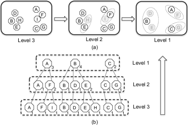
Figure 5: An illustration of the hierarchical clustering. There are 9 objects A-I, in decreasing order of importance. Each octagon is a cluster, with the representative object inside it. (a): Three zoom levels constructed. A dashed ellipse indicates the merging of the lighter cluster into the darker one. (b): A tree representation of the hierarchical clusters. The number next to a cluster is the number of objects this cluster represents. These numbers, along with other possible aggregation information, are computed when clusters merge.

Hierarchical clustering. The key part of the algorithm is a bottom-up hierarchical clustering process. Suppose there are $\eta$ zoom levels. We start with a fake bottom level $\eta+1$ where every object is in its own cluster. Each cluster’s aggregation information (e.g. aggregated stats and cluster boundaries) is initialized using the only object in it, which we call the “representative object” of a cluster in the following.

Then we build the clusters level by level. For each zoom level $i\in[1,\eta]$, we construct a new set of clusters by merging the clusters on level $i+1$. Zoom consistency (G3-c) is then guaranteed because each zoom level merges clusters from the one level down. By mathematical induction, we can show that if an object is visible on level $i$, it is visible on any level $j>i$.

Specifically, we iterate over all clusters on level $i+1$ in the order of the importance of their representative objects, which is a greedy strategy to make important objects more visible (G3-d). For each cluster $\alpha$ on level $i+1$, we search for a cluster $\beta$ on the current level $i$ with the closest $ncd$. If this $ncd$ is smaller than $\theta$, we merge $\alpha$ into $\beta$; otherwise we add $\alpha$ to level $i$. By merging a cluster into its nearest neighbor (measured in $ncd$), within-cluster variances can be reduced (G3-d). Figure 5 shows an example with 9 objects and 3 zoom levels.

Identifying outliers. The single-node algorithm preserves an outlier if it is not within $\theta$ $ncd$ of any other object. To identify less isolated outliers, one would need to assign to each object a score (i.e. the importance field) indicating how distant an object is from other objects. Kernel density estimations would be an example of such type of score.

Optimizations and complexity analysis. Let $n$ be the total number of objects. When constructing clusters for level $i$, sorting the clusters on level $i+1$ takes $O(n\log n)$. We maintain a spatial search tree (e.g. R-tree) of the clusters on level $i$ so that nearest neighbor searches can be done in $O(\log n)$. Inserting a new cluster into the tree also takes $O(\log n)$. Therefore, the overall time complexity of this algorithm is $O(n\log n)$ if we see the number of zoom levels as a constant.

6.3 A Multi-node Distributed Layout Algorithm

The algorithm presented in Section 6.2 only works on a single machine which has limited memory. Here, we extend it to work with a multi-node database system.

Given the sequential nature of the single-node algorithm, one major challenge here is how to utilize the parallelism offered by the multi-node database. Our idea is to spatially partition a zoom level, perform clustering in each partition independently in parallel and then merge the partitions. Figure 6 shows an illustration of the three steps. We detail them in the following, assuming the context of constructing clusters on zoom level $i$ from the clusters on level $i+1$.

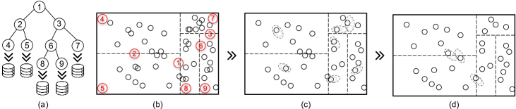
Figure 6: An illustration of the distributed clustering algorithm for zoom level $i$. (a), (b): clusters on zoom level $i+1$ are spatially partitioned and stored on multiple database nodes. KD-tree is used for skew-resilient partitioning. In (a), non-leaf tree nodes (1, 2, 3 and 6) represent KD-tree splits, while leaf tree nodes (4, 5, 7, 8 and 9) correspond to actual partitions. Each circle in (b) is a mark/cluster; (c): the single-node algorithm is run for each partition in parallel, merging clusters that have an $ncd$ smaller than $\theta$; (d): merging clusters close to partition boundaries.

Step 1: skew-resilient spatial partitioning. We use a KD-tree[8] to spatially partition the 2D plane so that each resulting partition has similar number of clusters from zoom level $i+1$. Note that each cluster belongs to exactly one partition according to its centroid. A KD-tree is a binary tree (Figure 6a) where every non-leaf tree node represents a split of a subplane, and every leaf tree node is a final partition stored as a table in one database node. KD-tree splits are axis-aligned and alternate between horizontal and vertical as one goes down the hierarchy. For each split, the median value of the corresponding axis is used as the split point. We stop splitting when the number of clusters in a partition can fit into the memory of one database node.

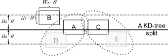
Figure 7: An example of merging clusters along a KD-tree split.

Step 2: processing partitions in parallel. Since each partition fits in the memory of one database node, we can efficiently run the single-node clustering algorithm on each partition in parallel. As a result, a new set of clusters is produced in each partition where no two clusters have an $ncd$ smaller than $\theta$ (Figure 6c).

Step 3: merging clusters on partition boundaries. After Step 2, some clusters close to partition boundaries may have an $ncd$ smaller than $\theta$. Step 3 resolves these border cases by merging clusters along KD-tree splits. We “process” (i.e. merging clusters along) KD-tree splits in a bottom-up fashion, starting with splits that connect two leaf partitions. After the KD-tree root is processed, we finish the layout generation for level $i$.

When processing a given split, we make use of the fact that only clusters whose centroid is within a certain distance to the split ($W_{B}\cdot\theta$ or $H_{B}\cdot\theta$ depending on the orientation of the split) need to be considered. Consider the horizontal split in Figure 7. The two horizontal dashed lines indicate the range of cluster centroids that we need to consider. Any cluster whose centroid is outside this range is at least $\theta$ away (in $ncd$) from any cluster on the other side of the split.

We use a greedy algorithm to process a KD-tree split. We iterate over all clusters in the aforementioned range in the order of their $x$ coordinates ($y$ if the split is vertical). We keep track of the last added/merged cluster $\alpha$. Let $\beta$ be the currently considered cluster. If $ncd(\alpha,\beta)\geq\theta$, we add $\beta$ and set $\alpha$ to $\beta$; otherwise we merge $\alpha$ and $\beta$. The one with the less important representative object is merged into the other (g3-d). Then we update $\alpha$ accordingly.

Consider again Figure 7. There are five clusters A-E in decreasing importance order. The boxes around clusters are their bounding boxes scaled by a factor of $\theta$. So if two boxes overlap, two corresponding clusters have an $ncd$ smaller than $\theta$ (see Figure 4). The above algorithm iterates over the clusters in the following order: $B,D,A,C,E$. When $\beta=A$, $\alpha=D$. $D$ is then merged into $A$ because $ncd(A,D)<\theta$ and $D$ has a less important representative object. For the same reason, $E$ is merged into $C$.

Optimizations and complexity analysis. Let $M$ be the upper bound on the number of clusters that can fit in memory. Hence there are roughly $T=\frac{n}{M}$ partitions, which means there are $O(T)$ KD-tree nodes. Determining the splitting point can be done in $O(\log n)$, thus constructing the spatial partitions takes $O(T\cdot\log n)$. Step 1 also involves distributing the clusters to the correct database node, which is often an expensive I/O bound process. So we do spatial partitioning only once based on the bottom level, and reuse the same partition scheme for other levels to avoid moving data around database nodes. Step 2 runs in $O(M\log M)$ because the single node algorithm is run in parallel across partitions. Step 3 takes $O(n\log T)$ because there are $\log T$ KD-tree levels in total, and we need to consider for each KD-tree level $n$ clusters in the worst case. However, Step 3 is expected to run very fast in practice because most clusters are out of the range in Figure 7.

Other partitioning strategies. One could partition the data using fields other than $x$ and $y$ and then in a similar fashion, run the single-node algorithm on the resulting partitions in parallel. However, since the two spatial attributes are not involved in partitioning, objects in each partition would span the whole 2D space. So even though overlap and density constraints are satisfied within each partition, when merged together, they will very likely be violated unless extra spatial postprocessing are in place. We therefore choose to perform spatial partitioning throughout to guarantee G3-a and G3-b.

6.4 Data Fetching

The data fetcher’s job is to efficiently fetch data in the user’s viewport (G4-b). We make use of multi-node spatial indexes, which can help fetch objects in a viewport-sized region with interactive response times.

Creating multi-node spatial indexes. Suppose the $j$-th ($1\leq j\leq T$) partition on zoom level $i$ is stored in the database table $t_{i,j}$, which has roughly $M$ clusters. We augment all such $t_{i,j}$ with a box-typed column bbox, which stores the bounding box of cluster marks. We then build a spatial index on column bbox, by issuing the following query:

⬇

CREATE INDEX sp_idx ON $t_{i,j}$ using gist(bbox);

where gist is the spatial index based on the generalized search tree[2]. In practice, these CREATE INDEX statements can be run in parallel by the multi-node database.

Fetching data from relevant partitions. Given a user viewport $V$ on zoom level $i$, clusters from partition $t_{i,j}$ that are inside $V$ can be fetched by a query like the following:

⬇

SELECT * FROM $t_{i,j}$ WHERE bbox && $V$;

where && is the intersection operator. The spatial index on bbox ensures that this query runs fast. We traverse the KD-tree to find out partitions that intersect $V$, run the above query on these partitions and union the results. Note that for top zoom levels that are small in size, there can be too many partitions that intersect with the viewport, which can be harmful for data fetching performance because we need to wait for sequential network trips to many database nodes. Therefore, we merge all partitions on each of the top $L$ levels into one database table. $L$ is an empirically determined constant based on the relative size of the zoom levels to the viewport size.

7 Implementation

We implement Kyrix-S as an extension to Kyrix[49], a general pan/zoom system we have built. This enables the developer to both rapidly author SSVs and reuse features of a general pan/zoom system in one integrated system. For example, Kyrix supports multiple coordinated views. Without switching tools, the developer can construct a multi-view visualization in which one or more views are SSVs authored with Kyrix-S. As another example, the developer can augment SSVs with the semantic zooming functionality provided by Kyrix, where the user can click on a visual mark and zoom into another SSV. Furthermore, Kyrix provides APIs for integrating a pan/zoom visualization into a web application, which are highly desired by the SSV developers we collaborate with. Examples include programmatic pan/zoom control, notifications of pan/zoom events, getting current visible data items.

Specification compilation. Kyrix-S uses a Node.js module to validate the JSON-based SSV specification. Validated specifications are compiled into low-level Kyrix specifications so that part of Kyrix’s frontend code can be reused to handle rendering and pan/zoom interactions.

Layout generator and data fetcher. Kyrix-S’s layout generator and data fetcher override respectively Kyrix’s index generator and data fetcher. Both components are written in the same Java application, using the Java Database Connectivity (JDBC) to talk to Citus, an open-source multi-node database built on top of PostgreSQL. The layout generator uses PLV8, a PostgreSQL extension that enables implementation of algorithms in Section 6 in Javascript functions, along with parallel execution of those functions directly inside each Citus database node.

Database deployment and orchestration. Kyrix-S provides useful scripts for one-command deployment of Kyrix-S and database dependencies (G1). We use Kubernetes to orchestrate a group of nodes running containerized Citus and Kyrix-S built with Docker.

Table 1: Online serving time (95-th percentile, in milliseconds).

	Reddit Text (Figure 1e, 1B objects)	Reddit Circle (Figure Kyrix-S: Authoring Scalable Scatterplot Visualizations of Big Data, 1B objects)	Taxi Heatmap (Figure 1a, 178.3M objects)	Taxi Contour (Figure 1b, 178.3M objects)	Liquor (Figure 1d, 17.3M objects)
Data Fetching	14	17	32	32	14
Network	1	1	223	254	1

Table 2: Offline indexing time (in minutes).

	Reddit Text (Figure 1e, 1B objects)	Reddit Circle (Figure Kyrix-S: Authoring Scalable Scatterplot Visualizations of Big Data, 1B objects)	Taxi Heatmap (Figure 1a, 178.3M objects)	Taxi Contour (Figure 1b, 178.3M objects)	Liquor (Figure 1d, 17.3M objects)
Building KD-tree (Step 1)	11.8	10.5	2.7	2.4	0.7
Redistributing data (Step 1)	94.3	100.0	8.5	8.4	1.3
Parallel clustering (Step 2)	9.9	3.7	6.9	9.0	4.7
Merge partitions (Step 3)	61.3	18.2	1.1	0.8	0.1
Creating Spatial Indexes	2.4	1.3	1.2	1.2	1.3
Total	179.7	133.8	20.3	21.8	8.2

8 Evaluation

We conducted extensive experiments to evaluate two aspects of Kyrix-S: 1) performance and 2) authoring effort.

8.1 Performance

We conducted performance experiments to evaluate the online serving and indexing performance of Kyrix-S. We used both example SSVs in Figures Kyrix-S: Authoring Scalable Scatterplot Visualizations of Big Data and 1 and a synthetic circle-based SSV Syn that visualizes a skewed dataset where 80% of the objects are in 20% of the 2D plane, and the rest of the 20% are uniformly distributed across the 2D plane. For database partitioning, we set $M=2$ million, i.e., each partition has roughly 2 million objects. So for a dataset with $N$ objects, there are $K=\left\lceil{\frac{N}{M}}\right\rceil$ partitions. Based on the number of partitions, we provision a Google Cloud Kubernetes cluster with $\left\lceil{\frac{K}{8}}\right\rceil$ n1-standard-8 PostgreSQL nodes (8 vCPUs, 30GB memory), each serving 8 partitions.

8.1.1 Online Serving Performance

To measure the online response times, we used a user trace where one pans around to find the most skewed region on a zoom level, zooms in, repeats until reaching the bottom level and then zooms all the way back to the top level. We measured the 95-th percentile of all data fetching time and network time.

Table 1 shows the results on five SSVs. The 95-percentile data fetching times were all below 32ms. The reason was because we only fetched data from the partitions that intersect with the viewport and the spatial indexes sped up the spatial queries. Network times were mostly negligible except for Taxi Heatmap and Taxi Contour, where many more data items were fetched due to smaller $\theta$ values.

Figure 8 shows the response times on different sizes of the synthetic SSV Syn. We can see that the response times remained stably under 20ms for data sizes from 32 million to 1 billion.

8.1.2 Offline Indexing Performance

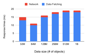
Figure 8: Serving scalability on the synthetic SSV Syn.

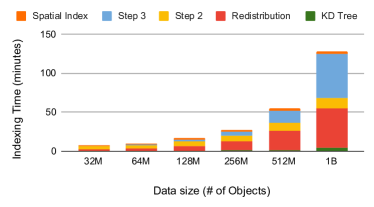
Figure 9: Indexing scalability on the synthetic SSV Syn.

Table 2 shows the indexing performance of the layout generator on five example SSVs. We make the following observations. First, the indexing phase finished in reasonable time: every example finished in less than 3 hours. Second, redistributing the data to the correct spatial partition was the most time consuming part since it was an I/O bound process. Fortunately, the same spatial partitions can be reused for updatable data if the spatial distribution does not change drastically. Third, parallel clustering and spatial index creation took the least time because they could be run in parallel across partitions. Fourth, merging clusters along KD-tree splits was mostly a cheap process. In fact, the largest number of clusters along a KD-tree split was 16,647. The reason that this step took longer on Reddit Text than on Reddit Circle was because it had more zoom levels (20 vs. 15) due to larger mark size (text vs. circle). Moreover, iterating through objects along KD-tree splits were much more time-consuming on the bottom five levels.

Figure 9 shows how indexing time changed for different sizes of Syn. We can see that the indexing time scaled well as the data size grew: as data size doubled, indexing time roughly doubled as well.

8.2 Authoring Effort

To evaluate the accessibility of our grammar, we compared the authoring effort of Kyrix-S with Kyrix[49], a state-of-the-art general pan/zoom system. To our best knowledge, Kyrix is the only system that offers declarative primitives for general pan/zoom visualizations, and has been shown to be accessible to visualization developers in a user study[49]. Former systems/languages such as D3[10], Pad++[5], Jazz[6] and ZVTM[45] require procedural programming which generally takes more authoring effort[49]. We measured lines of specifications using both systems for the two examples SSVs in Figures 1d and 1f. We used a code formatter to standardize the specifications, and only counted non-blank and non-comment lines.

Table 3: Comparison of lines of specifications when using Kyrix-S and Kyrix to author the two example SSVs in Figure 1d and Figure 1f.

	Kyrix-S	Kyrix	Kyrix-S’s saving over Kyrix
Figure 1d	62 lines	568 lines	$9.2\times$
Figure 1f w/ custom renderer	164 lines	610 lines	$3.7\times$
Figure 1f w/o custom renderer	68 lines	514 lines	$7.6\times$

Table 3 shows the results. We can see that when authoring the two example SSVs, Kyrix-S achieved respectively $9.2\times$ and $3.7\times$ saving in specifications compared to Kyrix. In the second example, when we excluded the custom renderer for soccer players (which has 96 lines), the amount of savings was $7.6\times$. These savings came from Kyrix-S abstracting away low-level details such as rendering of visual marks, configuring zoom levels, etc.

The above comparison did not include the code for layout generation. To enable the comparison, we stored the layouts generated by Kyrix-S as database tables so that Kyrix could directly use them. However, programming the layout was in fact a challenging task, as indicated by the total lines of code of Kyrix-S’s layout generator (1,439). Therefore, we conclude that Kyrix-S greatly reduced the user’s effort in authoring SSVs compared to general pan/zoom systems.

9 Limitations and Future Work

Other layout strategies. Kyrix-S’s assumes that the location of a mark comes from an object. This can be relaxed to diversify our layout generator. For example, supporting inexact placement of marks such as binned aggregation[24] in SSVs is one future direction. We also plan to investigate layout strategies that concern multi-class scatterplots, e.g. how to preserve relative density orders among multiple classes[11, 13].

More built-in templates. Our declarative grammar is designed to enable rapid extension of the system with custom marks. This motivates us to engage more with the open-source community and enrich our built-in mark gallery with templates commonly required/authored by developers.

Incremental updates. Currently, Kyrix-S assumes that data is static and pre-materialize mark layouts. To interactively debug, the developer needs to either use a sample of the data or reduce the number of zoom levels. It is our future work to identify ways to incrementally update our mark layout upon frequent changes of developer specifications, as well as when the data itself is updated dynamically.

Animated transitions. A discrete-zoom-level model simplifies layout generation, but can potentially lead to abrupt visual effect upon level switching, especially for KDE-based renderers such as heatmaps. As future work, we will use animated transitions to counter this limitation.

Raster Images-based SSVs. The visual density constraint, partly due to limited processing capabilities of the frontend and the database, forbids the creation of dense visualizations such as point clouds[44]. We envision the use of raster images to remove this constraint for these visualizations where interaction with objects is not required.

10 Conclusion

In this paper, we presented the design of Kyrix-S, a system for easy authoring of SSVs at scale. Kyrix-S contributed a declarative grammar that enabled concise specification of a wide range of SSVs and rapid authoring of custom marks. Behind the scenes, Kyrix-S automatically generated layout of visual marks on zoom levels using a range of usability guidelines such as maintaining a visual density budget and high data abstraction quality. To scale to big datasets, Kyrix-S worked with a multi-node parallel database system to implement the layout algorithm in a distributed setting. Multi-node spatial indexes were built to achieve interactive response times. We demonstrated the expressivity of Kyrix-S with a gallery of example SSVs. Experiments on real and synthetic datasets showed that Kyrix-S scaled to big datasets with billions of objects and reduced the authoring effort significantly compared to a state-of-the-art authoring system.

11 Acknowledgement

We thank the anonymous reviewers for their thoughtful feedback. This work was in part supported by NSF OAC-1940175, OAC-1939945, IIS-1452977, DGE-1855886, IIS-1850115, DARPA FA8750-17-2-0107 and the Data Systems and AI Lab initiative under Grant 3882825.

References

- [1] Leaflet markercluster plugin. https://github.com/Leaflet/Leaflet.markercluster. accessed: 2019/11.
- [2] Postgresql generalized search tree. https://www.postgresql.org/docs/12/textsearch-indexes.html. accessed: 2020/07.
- [3] Vega-lite javascript api. https://observablehq.com/@vega/vega-lite-api. accessed: 2019/11.
- [4] L. Battle, R. Chang, and M. Stonebraker. Dynamic Prefetching of Data Tiles for Interactive Visualization. In Proceedings of the 2016 International Conference on Management of Data, SIGMOD ’16, pp. 1363–1375. ACM, New York, NY, USA, 2016. doi: 10 . 1145/2882903 . 2882919
- [5] B. Bederson and J. Hollan. Pad++: a zooming graphical interface for exploring alternate interface physics. In Proceedings of the 7th annual ACM symposium on User interface software and technology, pp. 17–26. ACM, 1994.
- [6] B. Bederson, J. Meyer, and L. Good. Jazz: an extensible zoomable user interface graphics toolkit in java. In The Craft of Information Visualization, pp. 95–104. Elsevier, 2003.
- [7] C. Beilschmidt, T. Fober, M. Mattig, and B. Seeger. A linear-time algorithm for the aggregation and visualization of big spatial point data. In Proceedings of the 25th ACM SIGSPATIAL International Conference on Advances in Geographic Information Systems, p. 73. ACM, 2017.
- [8] J. L. Bentley. K-d trees for semidynamic point sets. In Proceedings of the sixth annual symposium on Computational geometry, pp. 187–197. ACM, 1990.
- [9] M. Bostock and J. Heer. Protovis: A graphical toolkit for visualization. IEEE Trans. Visualization & Comp. Graphics (Proc. InfoVis), 2009.
- [10] M. Bostock, V. Ogievetsky, and J. Heer. D3 data-driven documents. IEEE transactions on visualization and computer graphics, 17(12):2301–2309, 2011.
- [11] H. Chen, W. Chen, H. Mei, Z. Liu, K. Zhou, W. Chen, W. Gu, and K.-L. Ma. Visual abstraction and exploration of multi-class scatterplots. IEEE Transactions on Visualization and Computer Graphics, 20(12):1683–1692, 2014.
- [12] H. Chen, S. Engle, A. Joshi, E. D. Ragan, B. F. Yuksel, and L. Harrison. Using animation to alleviate overdraw in multiclass scatterplot matrices. In Proceedings of the 2018 CHI Conference on Human Factors in Computing Systems, p. 417. ACM, 2018.
- [13] X. Chen, T. Ge, J. Zhang, B. Chen, C.-W. Fu, O. Deussen, and Y. Wang. A recursive subdivision technique for sampling multi-class scatterplots. IEEE transactions on visualization and computer graphics, 2019.
- [14] Q. Cui, M. Ward, E. Rundensteiner, and J. Yang. Measuring data abstraction quality in multiresolution visualizations. IEEE Transactions on Visualization and Computer Graphics, 12(5):709–716, 2006.
- [15] A. Das Sarma, H. Lee, H. Gonzalez, J. Madhavan, and A. Halevy. Efficient spatial sampling of large geographical tables. In Proceedings of the 2012 ACM SIGMOD International Conference on Management of Data, pp. 193–204. ACM, 2012.
- [16] J.-Y. Delort. Vizualizing large spatial datasets in interactive maps. In 2010 Second International Conference on Advanced Geographic Information Systems, Applications, and Services, pp. 33–38. IEEE, 2010.
- [17] M. Derthick, M. G. Christel, A. G. Hauptmann, and H. D. Wactlar. Constant density displays using diversity sampling. In IEEE Symposium on Information Visualization 2003 (IEEE Cat. No. 03TH8714), pp. 137–144. IEEE, 2003.
- [18] A. Dix and G. Ellis. By chance enhancing interaction with large data sets through statistical sampling. In Proceedings of the Working Conference on Advanced Visual Interfaces, pp. 167–176. ACM, 2002.
- [19] M. Drosou and E. Pitoura. Disc diversity: result diversification based on dissimilarity and coverage. Proceedings of the VLDB Endowment, 6(1):13–24, 2012.
- [20] G. Ellis and A. Dix. A taxonomy of clutter reduction for information visualisation. IEEE transactions on visualization and computer graphics, 13(6):1216–1223, 2007.
- [21] N. Elmqvist and J.-D. Fekete. Hierarchical aggregation for information visualization: Overview, techniques, and design guidelines. IEEE Transactions on Visualization and Computer Graphics, 16(3):439–454, 2009.
- [22] J.-D. Fekete and C. Plaisant. Interactive information visualization of a million items. In IEEE Symposium on Information Visualization, 2002. INFOVIS 2002., pp. 117–124. IEEE, 2002.
- [23] T. Guo, K. Feng, G. Cong, and Z. Bao. Efficient selection of geospatial data on maps for interactive and visualized exploration. In Proceedings of the 2018 International Conference on Management of Data, pp. 567–582. ACM, 2018.
- [24] F. Heimerl, C.-C. Chang, A. Sarikaya, and M. Gleicher. Visual designs for binned aggregation of multi-class scatterplots. arXiv preprint arXiv:1810.02445, 2018.
- [25] J. Jo, F. Vernier, P. Dragicevic, and J.-D. Fekete. A declarative rendering model for multiclass density maps. IEEE Transactions on Visualization and Computer Graphics, 25(1):470–480, 2018.
- [26] S. Jul and G. W. Furnas. Critical zones in desert fog: aids to multiscale navigation. In Proceedings of the 11th annual ACM symposium on User interface software and technology, pp. 97–106. ACM, 1998.
- [27] P. K. Kefaloukos, M. V. Salles, and M. Zachariasen. Declarative cartography: In-database map generalization of geospatial datasets. In 2014 IEEE 30th International Conference on Data Engineering, pp. 1024–1035. IEEE, 2014.
- [28] D. A. Keim and A. Herrmann. The gridfit algorithm: An efficient and effective approach to visualizing large amounts of spatial data. IEEE, 1998.
- [29] D. E. Knuth. Backus normal form vs. backus naur form. Communications of the ACM, 7(12):735–736, 1964.
- [30] R. Kosara, S. Miksch, and H. Hauser. Focus+ context taken literally. IEEE Computer Graphics and Applications, 22(1):22–29, 2002.
- [31] F. Lekschas, M. Behrisch, B. Bach, P. Kerpedjiev, N. Gehlenborg, and H. Pfister. Pattern-driven navigation in 2d multiscale visualizations with scalable insets. IEEE transactions on visualization and computer graphics, 2019.
- [32] H. Liao, Y. Wu, L. Chen, and W. Chen. Cluster-based visual abstraction for multivariate scatterplots. IEEE transactions on visualization and computer graphics, 24(9):2531–2545, 2017.
- [33] L. Lins, J. T. Klosowski, and C. Scheidegger. Nanocubes for real-time exploration of spatiotemporal datasets. IEEE Transactions on Visualization and Computer Graphics, 19(12):2456–2465, 2013.
- [34] C. Liu, C. Wu, H. Shao, and X. Yuan. Smartcube: An adaptive data management architecture for the real-time visualization of spatiotemporal datasets. IEEE transactions on visualization and computer graphics, 2019.
- [35] Z. Liu and J. Heer. The effects of interactive latency on exploratory visual analysis. IEEE transactions on visualization and computer graphics, 20(12):2122–2131, 2014.
- [36] Z. Liu, B. Jiang, and J. Heer. immens: Real-time visual querying of big data. In Computer Graphics Forum, vol. 32, pp. 421–430. Wiley Online Library, 2013.
- [37] A. Mayorga and M. Gleicher. Splatterplots: Overcoming overdraw in scatter plots. IEEE transactions on visualization and computer graphics, 19(9):1526–1538, 2013.
- [38] F. Miranda, L. Lins, J. T. Klosowski, and C. T. Silva. Topkube: a rank-aware data cube for real-time exploration of spatiotemporal data. IEEE Transactions on visualization and computer graphics, 24(3):1394–1407, 2017.
- [39] D. Moritz, B. Howe, and J. Heer. Falcon: Balancing interactive latency and resolution sensitivity for scalable linked visualizations. In Proceedings of the 2019 CHI Conference on Human Factors in Computing Systems, p. 694. ACM, 2019.
- [40] S. Nutanong, M. D. Adelfio, and H. Samet. Multiresolution select-distinct queries on large geographic point sets. In Proceedings of the 20th International Conference on Advances in Geographic Information Systems, pp. 159–168. ACM, 2012.
- [41] C. A. Pahins, S. A. Stephens, C. Scheidegger, and J. L. Comba. Hashedcubes: Simple, low memory, real-time visual exploration of big data. IEEE transactions on visualization and computer graphics, 23(1):671–680, 2016.
- [42] D. Park, S. M. Drucker, R. Fernandez, and N. Elmqvist. Atom: A grammar for unit visualizations. IEEE transactions on visualization and computer graphics, 24(12):3032–3043, 2017.
- [43] A. Perrot, R. Bourqui, N. Hanusse, F. Lalanne, and D. Auber. Large interactive visualization of density functions on big data infrastructure. In 2015 IEEE 5th Symposium on large Data Analysis and Visualization (lDAV), pp. 99–106. IEEE, 2015.
- [44] C. Philippe, R. Jonas, F. Jean-Daniel, L. Anne-Catherine, and S. Michèle. Cartolabe: A web-based scalable visualization of large document collections. arXiv preprint arXiv:2003.00975, 2020.
- [45] E. Pietriga. A toolkit for addressing hci issues in visual language environments. In null, pp. 145–152. IEEE, 2005.
- [46] A. Sarikaya and M. Gleicher. Scatterplots: Tasks, data, and designs. IEEE transactions on visualization and computer graphics, 24(1):402–412, 2017.
- [47] A. Satyanarayan, D. Moritz, K. Wongsuphasawat, and J. Heer. Vega-lite: A grammar of interactive graphics. IEEE Trans. Visualization & Comp. Graphics (Proc. InfoVis), 2017.
- [48] A. Satyanarayan, K. Wongsuphasawat, and J. Heer. Declarative interaction design for data visualization. In ACM User Interface Software & Technology (UIST), 2014.
- [49] W. Tao, X. Liu, Y. Wang, L. Battle, Ç. Demiralp, R. Chang, and M. Stonebraker. Kyrix: Interactive pan/zoom visualizations at scale. In Computer Graphics Forum, vol. 38, pp. 529–540. Wiley Online Library, 2019.
- [50] M. Trutschl, G. Grinstein, and U. Cvek. Intelligently resolving point occlusion. In IEEE Symposium on Information Visualization 2003 (IEEE Cat. No. 03TH8714), pp. 131–136. IEEE, 2003.
- [51] C. Waldeck and D. Balfanz. Mobile liquid 2d scatter space (ml2dss). In Proceedings. Eighth International Conference on Information Visualisation, 2004. IV 2004., pp. 494–498. IEEE, 2004.
- [52] H. Wickham. ggplot2: Elegant Graphics for Data Analysis. Springer-Verlag New York, 2009.
- [53] H. Wickham. A layered grammar of graphics. Journal of Computational and Graphical Statistics, 19(1):3–28, 2010.
- [54] J. Yang, M. O. Ward, and E. A. Rundensteiner. Interactive hierarchical displays: a general framework for visualization and exploration of large multivariate data sets. Computers & Graphics, 27(2):265–283, 2003.