Three identical bosons: Properties in non-integer dimensions and in external fields

Abstract

Three-body systems that are continuously squeezed from a three-dimensional (3D) space into a two-dimensional (2D) space are investigated. Such a squeezing can be obtained by means of an external confining potential acting along a single axis. However, this procedure can be numerically demanding, or even undoable, especially for large squeezed scenarios. An alternative is provided by use of the dimension $d$ as a parameter that changes continuously within the range $2\leq d\leq 3$. The simplicity of the $d$-calculations is exploited to investigate the evolution of three-body states after progressive confinement. The case of three identical spinless bosons with relative $s$-waves in 3D, and a harmonic oscillator squeezing potential is considered. We compare results from the two methods and provide a translation between them, relating dimension, squeezing length, and wave functions from both methods. All calculations are then possible entirely within the simpler $d$-method, but simultaneously providing the equivalent geometry with the external potential.

I Introduction

Specific cold atomic or molecular gases can be controlled by external fields to previously unprecedented accuracy blo08 ; den16 . This manipulation consists of two relevant ingredients, i.e., (i) the two-body effective interactions can be varied continuously between strong attraction and strong repulsion, still while the system is confined by an external trap, and (ii) the geometric space allowed by the particles can be designed at will and restricted to large volumes in three dimensions (3D), flat or curved surfaces (2D), linear (1D), or anything between these geometries. The properties of the systems differ substantially depending on the confinement, which in practice can be varied by use of an external deformed potential, where one or more dimensions can be squeezed down to vanishing size.

Together with the dimension, $d$, the properties depend as well on the number of particles arm15 . However, so far only the $d$-dependence of the relative motion of the simplest systems has been studied by various methods yam15 ; san18 ; moe19 . Two particles squeezed between integer dimensions are obviously the simplest case, but beside its inherent interest, it is also necessary in investigations of three particles. One advantage is that the two masses only enter in the relative motion as the reduced mass, and only as a factor in the overall scale parameter. This is reported in previous papers using both momentum-space coordinates san18 ; ros18 and ordinary space coordinates lev14 ; gar19a ; gar19b .

Recently, a $d$-dependent formulation has been presented and applied to two-body systems gar19a ; gar19b . The basic assumption is to use $d$ as a parameter that can take non-integer values, in such a way that the external squeezing potential does not appear at all, but is instead substituted by the correspondingly modified Schrödinger equation depending on $d$ and particle number, $N$ nie01 ; jen04 . The required numerical effort is similar to a standard calculation for an integer dimension, but where the external potential has disappeared. In these works, gar19a ; gar19b , the equivalence between the $d$-dependent method and the more direct procedure working in three dimensions including explicitly the external squeezing potential was investigated. For the case of a squeezing harmonic oscillator potential a connection between the oscillator length and the equivalent dimension $d$ was found.

In this work we extend the method presented in gar19a ; gar19b to three-body systems. First, we describe in Section II how the hyperspherical adiabatic expansion method can be implemented to study three-body systems in a $d$-dimensional space. In Section III we then describe how the adiabatic expansion can be used as well to treat the same problem in a direct way, i.e., describing the system in 3D, but introducing explicitly the external squeezing potential. This procedure, although formally not very complicated, often leads to calculations that, specially for large squeezing, are out of numerical reach. The connection between the dimension and the external field, and the interpretation of the $d$-dimensional wave function are described in Sections IV and V, respectively.

The two methods are applied to systems made of three identical spinless bosons and relative $s$-waves in 3D. In Section VI we specify the applied two-body potentials giving rise to different three-body scenarios. In Sections VII and VIII the evolution of the three-body bound states after progressive squeezing is investigated for each of the two methods. A translation between the parameter, $d$, and the squeezing potential is investigated in Section IX, where the wave function in $d$ dimensions is interpreted as a deformed wave function in the ordinary 3D-space. We close in Section X with the summary and the conclusions.

II Three bosons in $d$-dimensions

From a general perspective, the description of a given $N$-body system requires solving the Schrödinger equation

$$\bigg{[}-\sum_{i=1}^{N}\frac{\hbar^{2}}{2m_{i}}\Delta_{\bm{r_{i}}}+\frac{\hbar^{2}}{2M}\Delta_{\bm{R}_{cm}}+\sum_{i<j}V_{k}(\bm{r}_{ij})-E_{Nb}\bigg{]}\Psi=0\;,$$ (1)

where $m_{i}$ and $\bm{r}_{i}$ are mass and position vector of particle $i$, respectively, $M=\sum m_{i}$ is the total mass, and $\bm{R}_{cm}$ is the $N$-body center-of-mass coordinate. The kinetic energy due to the center-of-mass motion is then explicitly removed. The potential $V_{k}(\bm{r}_{ij})$ is the interaction between particles $i$ and $j$, which is assumed to depend on the relative vector, $\bm{r}_{ij}$, between the two particles. Finally, $E_{Nb}$ is the total $N$-body energy.

The one-body kinetic energy operator for $N$ particles can be expressed in terms of the hyperradius, $\rho$, and all the remaining necessary angles, the hyperangles, related to the relative degrees of freedom jen04 . The square, $\rho^{2}$, of the hyperradius is defined in terms of the particle coordinates and the arbitrary normalization mass, $m$, as:

$$\rho^{2}=\frac{1}{m}\sum_{i=1}^{N}m_{i}\left(\bm{r}_{i}-\bm{R}_{cm}\right)^{2}=\sum_{i<j}\frac{m_{i}m_{j}}{mM}(\bm{r}_{i}-\bm{r}_{j})^{2},$$ (2)

which can be separated into the Cartesian coordinate contributions, i.e.

$$\rho^{2}=\rho_{x}^{2}+\rho_{y}^{2}+\rho_{z}^{2}.$$ (3)

The hyperradial part of the reduced equation of motion has the usual second derivative operator and a centrifugal term, $(f-1)(f-3)/(4\rho^{2})$, where $f$ is the number of relative degrees of freedom. For a given $N$-body system in a general $d$-dimensional space it is then clear that $f=d(N-1)$, which results in the equation of motion in $d$ dimensions given in jen04 , i.e.

$$\bigg{[}-\frac{\partial^{2}}{\partial\rho^{2}} + \frac{\ell_{d,N}(\ell_{d,N}+1)+\hat{\Lambda}_{d,N}^{2}(\Omega_{d,N})}{\rho^{2}}+$$

$$+ \frac{2m}{\hbar^{2}}\sum_{i<j}V_{k}(\bm{r}_{ij})-\frac{2mE_{d,N}}{\hbar^{2}}\bigg{]}\psi_{d,N}=0\;,$$

where the generalized angular momentum quantum number, $\ell_{d,N}$, is given by

$$\ell_{d,N}=\frac{f-3}{2}=\frac{1}{2}(d(N-1)-3),$$ (5)

and where $\hat{\Lambda}_{d,N}^{2}$, which depends on the hyperangles $\Omega_{d,N}$, is the generalization to $N$ particles and $d$ dimensions of the usual hypermomentum operator nie01 . The energy $E_{Nb}$ in Eq.(1) is denoted now as $E_{d,N}$, making explicit the dependence on the dimension. Finally, the phase space reduced wave function, $\psi_{d,N}$, is expressed in terms of the total wave function $\Psi_{d,N}$ as

$$\psi_{d,N}=\rho^{\ell_{d,N}+1}\Psi_{d,N}\;.$$ (6)

Once the two-body interaction potentials, $V_{k}$, are defined, different procedures can be used to reduce Eq.(II) to a set of equations depending only on the hyperradius gar18 . The key in all of them consists in expanding the wave function in a certain basis set that contains the whole dependence on the hyperangles (for instance the eigenfunctions of the $\hat{\Lambda}_{d,N}^{2}$-operator), in such a way that projection of Eq.(II) on the different basis terms immediately leads to a couple set of differential equations for the radial function coefficients.

II.1 The three-body case

Being more specific, and focusing on three-body systems, $N=3$, the total three-body wave function in $d$ dimensions will be obtained in this work by solving the Faddeev equations leading to the Schrödinger equation (II). In particular, the wave function is written as:

$$\Psi_{d}=\frac{\psi_{d}}{\rho^{\frac{2d-1}{2}}}=\frac{1}{\rho^{\frac{2d-1}{2}}}\sum_{n}f_{n}^{(d)}(\rho)\sum_{i=1}^{3}\Phi_{n}^{(d,i)}(\Omega_{d}),$$ (7)

where $\Psi_{d}\equiv\Psi_{d,3}$, and where the angular functions, $\Phi_{n}^{(d,i)}$, which form a complete basis set, are the eigenfunctions, with eigenvalue $\lambda^{(d)}_{n}(\rho)$, of the $d$-dependent angular part of the Faddeev equations (see nie01 for details).

Once the angular part has been solved, projection of Eq.(II) on these angular functions leads to the following coupled set of differential equations from which the radial wave functions $f_{n}^{(d)}$ in the expansion (7) can be obtained:

$$\left[-\frac{\partial^{2}}{\partial\rho^{2}}+\frac{1}{\rho^{2}}\left(\lambda_{n}^{(d)}(\rho)+\frac{(2d-3)(2d-1)}{4}\right)-\frac{2mE_{d}}{\hbar^{2}}\right]f_{n}^{(d)}(\rho)$$ (8)

$$=\sum_{n^{\prime}}\left(2P_{nn^{\prime}}(\rho)\frac{\partial}{\partial\rho}+Q_{nn^{\prime}}(\rho)\right)f_{n^{\prime}}^{(d)}(\rho),$$

where the angular eigenvalues $\lambda_{n}^{(d)}(\rho)$ enter as effective potentials, the explicit form of the coupling terms $P_{nn^{\prime}}$ and $Q_{nn^{\prime}}$ can be found in nie01 , and where $E_{d}$ is the energy of the three-body system moving in the $d$-dimensional space ($E_{d}\equiv E_{d,3}$).

The method used is just the hyperspherical adiabatic expansion method, derived in detail in Ref.nie01 for any arbitrary dimension $d$. The generalization of the spherical harmonics to $d$ dimensions can be found for instance in Appendix B of Ref.nie01 . They depend on the $d-1$ angles needed to specify the direction of a given vector coordinate in $d$ dimensions. This of course makes sense for integer values of $d$, which leads to an integer number of well-defined angles (for instance two angles for $d=3$ or one angle for $d=2$). However, when $d$ is allowed to take non-integer values, the definition of the angles and therefore the definition of the spherical harmonics is not obvious.

To overcome this problem we shall restrict ourselves to $s$-waves, i.e. zero relative orbital angular momenta between the particles. In this way the angular dependence of the spherical harmonics disappears (see Appendix A).

III Harmonic Confinement

The method presented in the previous section appears as an alternative to the natural way of confining an $N$-particle system, which is to put it under the effect of an external potential that forces the particles to move in a limited region of space. Therefore, from the theoretical point of view, the problem to be solved is just the one given in Eq.(1) applied in 3D, but where both the interaction between particles, $\sum_{i<j}V_{k}$, and the trap potential, $V_{trap}$, have to be included.

An important point to keep in mind is that the energy $E_{Nb}$ in Eq.(1) is now the total $N$-body energy, in such a way that the energy of the squeezed system requires subtraction of the (diverging for $d\rightarrow 2$) zero-point energy of an $N$-body system trapped by the potential $V_{trap}$.

In this work we shall consider an external harmonic oscillator potential acting along the $z$-direction. The frequency of the potential will be written as:

$$\omega=\frac{\hbar}{m_{\omega}b_{ho}^{2}},$$ (9)

where $m_{\omega}$ is some arbitrary mass, and $b_{ho}$ will be referred to as the harmonic oscillator length parameter. Obviously, the smaller $b_{ho}$ the more confined the particles, and, eventually, for $b_{ho}=0$ the particles can move only in a 2D-space.

The relative trap potential (the center-of-mass part is separated and omitted) can therefore be written as

$$V_{trap}=\frac{1}{2}\omega^{2}\sum_{i=1}^{N}m_{i}\left(z_{i}-Z_{cm}\right)^{2},$$ (10)

where $z_{i}$ and $Z_{cm}$ are the $z$-components of $\bm{r}_{i}$ and $\bm{R}_{cm}$, respectively, and where $Z_{cm}$, together with the kinetic energy term $\hbar^{2}\Delta_{\bm{R}_{cm}}/2M$ in Eq.(1), is introduced to remove the contribution from the center-of-mass motion.

The squeezing potential can be written in a more compact way as

$$V_{trap}=\frac{1}{2}m\omega^{2}\rho_{z}^{2},$$ (11)

where $m$ is the arbitrary normalization mass introduced in Eq.(2), and $\rho_{z}^{2}$ refers to the $z$-contribution of the square of the generalized hyperradius vector size defined in Eqs.(2) and (3).

For this particular case, and making more specific the discussion above, the energy of the squeezed system is given by $E_{ext}=E_{Nb}-E_{ho}$, where $E_{ho}=(N-1)\hbar\omega/2$ is the zero-point energy in the one dimensional squeezed oscillator for the $N-1$ relative degrees of freedom.

III.1 The three-body case

Let us focus now on the three-body case, and let us assume an external harmonic oscillator one-body squeezing potential which, as in Eqs.(10) and (11), acts along the $z$-axis. From the definition of the $\bm{x}$ and $\bm{y}$ Jacobi coordinates nie01 , it is not difficult to see that the trap potential felt by the three particles can be written as:

$$\frac{1}{2}\omega^{2}\sum_{i=1}^{3}m_{i}r_{i}^{2}\cos^{2}\theta_{i}=\frac{1}{2}m\omega^{2}x^{2}\cos^{2}\theta_{x}+$$

$$+\frac{1}{2}m\omega^{2}y^{2}\cos^{2}\theta_{y}+\frac{1}{2}M\omega^{2}R_{cm}^{2}\cos^{2}\theta_{cm},$$

where $\theta_{x}$ and $\theta_{y}$ are the polar angles associated to the $\bm{x}$ and $\bm{y}$ Jacobi coordinates, respectively.

Therefore, after removal of the three-body center of mass motion the total trap potential takes the form:

$$V_{trap}(x,y,\theta_{x},\theta_{y})=\frac{1}{2}m\omega^{2}x^{2}\cos^{2}\theta_{x}+\frac{1}{2}m\omega^{2}y^{2}\cos^{2}\theta_{y},$$ (13)

which is nothing but the particularization to three particles of Eq.(11).

A more convenient way of writing the trap potential can be obtained by working from the beginning in the three-body center-of-mass. This means that all coordinates are measured relative to the center-of-mass, $\bm{R}_{cm}$. In turn, this implies that the coordinate $\bm{r}_{i}-\bm{R}_{cm}$ corresponding to particle $i$ is proportional to the $\bm{y}$-Jacobi coordinate in the Jacobi set $i$. Formally, we can then insert $\bm{R}_{cm}=0$, and in the center-of-mass system arrive at, see nie01

$$\bm{r}_{i}=\sqrt{\frac{m}{m_{i}}}\sqrt{\frac{m_{j}+m_{k}}{m_{i}+m_{j}+m_{k}}}\bm{y}_{i},$$ (14)

from which the potential in Eq.(III.1), or Eq.(13), can also be written as:

$$V_{trap}=\sum_{i=1}^{3}V_{trap}^{(i)}=\frac{1}{2}m\omega^{2}\sum_{i=1}^{3}\frac{m_{j}+m_{k}}{m_{i}+m_{j}+m_{k}}y_{i}^{2}\cos^{2}\theta_{y_{i}}.$$ (15)

This last form of the squeezing potential is particularly useful when, instead of solving directly the Schrödinger equation (1), the equation is split into its three Faddeev components.

The numerical procedure will be the same as the one shown in the previous section, i.e., we solve the Faddeev equations in coordinate space by means of the hyperspherical adiabatic expansion method described in nie01 . The full calculation is now performed in 3D, and therefore the three-body wave function will be written as in Eq.(7) but with $d=3$, that is:

$$\Psi_{ext}=\frac{1}{\rho^{5/2}}\sum_{n}f_{n}(\rho)\sum_{i=1}^{3}\Phi_{n}^{(i)}(\rho,\Omega_{i}),$$ (16)

where $\rho$ is the hyperradius and $\Omega_{i}$ collects the five hyperangles associated to the Jacobi coordinates $\{\bm{x}_{i},\bm{y}_{i}\}$, where $i$ runs over the three possible Jacobi sets nie01 .

Again, the angular functions $\Phi_{n}^{(i)}$ are obtained as the eigenfunctions of the angular part of the Faddeev equations, and, as in the previous section, the radial wave functions $f_{n}(\rho)$ in the expansion Eq.(16) are obtained after solving the coupled set of radial equations (8), but now particularized for $d=3$. The energy obtained in this way, $E_{3b}$, is the total energy, system plus external field, in such a way that the energy of the confined system will be obtained after subtraction of the harmonic oscillator energy, i.e., $E_{ext}=E_{3b}-E_{ho}$, which in our case of squeezing two coordinates along one direction, see Eq.(13), means $E_{ext}=E_{3b}-\hbar\omega$.

As shown in nie01 , the angular functions $\Phi_{n}^{(i)}$ are obtained after expanding them in terms of the hyperspherical harmonics. Calculation of the $\rho$-dependent coefficients in this expansion requires calculation of the matrix elements of the full potential in between all the hyperspherical harmonics included in the basis set. Due to the presence of the squeezing term (15), the calculation of these matrix elements involves calculation of the integral

$$W_{\ell_{x}\ell_{y}LM}^{\ell^{\prime}_{x}\ell^{\prime}_{y}L^{\prime}M^{\prime}}=\int d\Omega_{x}d\Omega_{y}\left[Y^{*}_{\ell_{x}}(\Omega_{x})\otimes Y^{*}_{\ell_{y}}(\Omega_{y})\right]^{LM}$$ (17)

$$\times\cos^{2}\theta_{y}\left[Y_{\ell^{\prime}_{x}}(\Omega_{x})\otimes Y_{\ell^{\prime}_{y}}(\Omega_{y})\right]^{L^{\prime}M^{\prime}},$$

where $\ell_{x}$ and $\ell_{y}$ are the orbital angular momenta associated to the Jacobi coordinates $\bm{x}$ and $\bm{y}$, respectively, which couple to the total angular momentum $L$. For simplicity in the notation, we have assumed spinless particles, although the generalization to particles with non-zero spin is straightforward.

The integral in Eq.(17) is analytical, and it takes the form:

$$W_{\ell_{x}\ell_{y}LM}^{\ell^{\prime}_{x}\ell^{\prime}_{y}L^{\prime}M^{\prime}}=$$ (27)

$$\delta_{\ell_{x}\ell^{\prime}_{x}}\delta_{MM^{\prime}}\sum_{\tilde{L}}(-1)^{\ell_{x}+M}(2\tilde{L}+1)\hat{L}\hat{L^{\prime}}\hat{\ell_{y}}\hat{\ell^{\prime}_{y}}\left(\begin{array}[]{ccc}1&1&\tilde{L}\\ 0&0&0\end{array}\right)^{2}$$

$$\times\left(\begin{array}[]{ccc}\ell_{y}&\tilde{L}&\ell^{\prime}_{y}\\ 0&0&0\end{array}\right)\left(\begin{array}[]{ccc}L&\tilde{L}&L^{\prime}\\ -M&0&M\end{array}\right)\left\{\begin{array}[]{ccc}L&\tilde{L}&L^{\prime}\\ \ell^{\prime}_{y}&\ell_{x}&\ell_{y}\end{array}\right\},$$

where $\hat{\ell}$ means $\sqrt{2\ell+1}$.

Therefore, the integral Eq.(17), or, in other words, the trap potential Eq.(15), mixes the relative angular momenta $\ell_{y}$ and $\ell^{\prime}_{y}$, and the total angular momenta $L$ and $L^{\prime}$, which is then not a good quantum number (unless the trap potential is equal to zero). The projections $M$ and $M^{\prime}$ are not mixed, and its conserved value determines the 2D angular momentum after an infinite squeezing of the particles along the $z$-axis.

In this work we shall consider the case of three identical spinless bosons, and for the case of no squeezing only $s$-waves will be considered. In other words, in 3D the system will have quantum numbers $L=0$ and $M=0$, which implies that, all along the squeezing process, the conserved quantum number $M$ will be equal to 0.

IV Trap versus $d$-parameter

The practical use of the $d$-formalism described in Section II depends on how to relate to parameters used in the laboratory setup. A universal connection was established for any two-body system squeezed from three to two dimensions by an external one-body oscillator field gar19a ; gar19b . The provided relationship then allows to use the parameter $d$ in the calculation and uniquely relate to an oscillator frequency or length parameter, or in principle vice versa.

We would like to generalize to three-body systems, but the degrees of freedom and related structures are now much larger. To begin this search we start with the very general formulation of $N$ two-body interacting particles. As described in the previous two sections, the controlling equations are described in terms of hyperspherical coordinates, where the hyperradius is the most important coordinate in a widely applicable expression. The reason is that, if the hyperangles were important, the internal $N$-body structure would influence the connection. This in turn can only appear through a complicated interpretation of the “spherical” wave function in the $d$-calculation.

To understand the relation between $d$ and $b_{ho}$ a little better, we use a simple model with an oscillator as the internal two-body interaction. Therefore, the sum of the two-body interactions entering in Eqs.(1) and (II) takes the form:

$$\sum_{i<j}V_{k}(\bm{r}_{ij}) = \frac{\omega_{pp}^{2}}{2M}\sum_{i<j}m_{i}m_{j}(\bm{r}_{i}-\bm{r}_{j})^{2}\;$$

$$= \frac{1}{2}m\omega_{pp}^{2}\rho^{2}\;,$$

where Eq.(2) has been used, and where $\omega_{pp}$ describes the strength of the given particle-particle interaction.

Eqs.(1) and (II) are then pure harmonic oscillator equations, and the corresponding energy solutions for the $d$-calculation and the calculation with external field, respectively, are arm15

$$E_{d}=\hbar\omega_{pp}(\ell_{d,N}+3/2)=\frac{1}{2}d(N-1)\hbar\omega_{pp}$$ (29)

where Eq.(5) has been used, and

$$E_{ext} = \hbar\omega_{pp}(N-1)$$

$$+ \frac{(N-1)}{2}\hbar\sqrt{\omega_{pp}^{2}+\omega^{2}}-\hbar\omega\frac{(N-1)}{2}\;,$$

where the first term is from the two non-squeezed perpendicular directions, the second term is from the squeezed direction, and the last term removes the diverging zero-point energy. The factor $N-1$ on all terms refer to the number of relative degrees of freedom for $N$ particles. The two limits of $\omega=0$ and $\omega=\infty$ produce the oscillator results corresponding to $d=3$ and $d=2$.

If the two procedures are assumed to be equivalent, we then must have that the expressions in Eqs.(29) and (IV) have to be equal, which after division throughout by $\hbar\omega_{pp}$ results in

$$d=2+\sqrt{1+\omega^{2}/\omega_{pp}^{2}}-\omega/\omega_{pp}\;,$$ (31)

and

$$\frac{\omega}{\omega_{pp}}=\frac{b_{pp}^{2}}{b_{ho}^{2}}=-\frac{(d-1)(d-3)}{2(d-2)}\;,$$ (32)

where $b_{pp}^{2}=\hbar/(m\omega_{pp})$ and $m_{\omega}$ in Eq.(9) is taken $m_{\omega}=m$. This relation is independent of the number of particles, $N$, and it is only an average estimate where all structure is absent. This observation is perhaps enhanced by having three identical bosons in the ground state.

The relation given in Eq.(32) reveals the correct limit at the initial and final dimensions, that means the squeezing length $b_{ho}$ approaches infinity or zero, respectively, for the cases of no squeezing ($d=3$) or infinite squeezing ($d=2$). Also these results and conclusions could be achieved from working directly with the special cases of the present interest $N=2$ and $3$.

When using the harmonic oscillator two-body potentials in Eq.(IV), beside the energies Eqs.(29) and (IV), the wave functions, solutions of Eqs.(1) and (II), are also available for the two methods. They are very different in structure, since one is spherical but in $d$ dimensions, and the other is deformed in three dimensions. The ground states are Gaussians in both cases corresponding to oscillators.

In particular, for the $d$-calculation, the $N$-body ground state oscillator wave function, $\Psi_{N,d}$, is a Gaussian, which is

$$\Psi_{d,N}\propto\exp{\left(-\frac{\rho^{2}}{2b_{pp}^{2}}\right)},$$ (33)

where $b_{pp}$, as defined below Eq.(32), is the oscillator length associated to the two-body interaction (IV).

Similarly, for the case of confinement with an external field, the ground state oscillator wave function, $\Psi_{ext}$, is also a Gaussian:

$$\Psi_{ext}\propto\exp{\left(-\frac{\rho_{\perp}^{2}}{2b_{\perp}^{2}}\right)}\exp{\left(-\frac{\rho_{z}^{2}}{2b_{z}^{2}}\right)},$$ (34)

where the oscillator lengths are

$$b_{z}^{2}=\frac{\hbar}{m\sqrt{\omega_{pp}^{2}+\omega^{2}}},$$ (35)

coming from the combination of the two-body and the squeezing oscillators acting along the $z$-axis, and

$$b_{\perp}^{2}=b_{pp}^{2}=\frac{\hbar}{m\omega_{pp}},$$ (36)

which results from the two-body oscillator acting on the plane perpendicular to the $z$-axis, and where $\rho_{\perp}$ and $\rho_{z}$ are defined as:

$$\rho_{\perp}^{2}=x_{\perp}^{2}+y_{\perp}^{2};\hskip 28.45274pt\rho_{z}^{2}=x_{z}^{2}+y_{z}^{2},$$ (37)

with $\{x_{z},y_{z}\}$ and $\{x_{\perp},y_{\perp}\}$ being, respectively, the $z$ and perpendicular components of the Jacobi coordinates $\{\bm{x},\bm{y}\}$.

Assuming equality between the wave functions in Eqs.(33) and (34) from the two methods we infer that the perpendicular length scale should remain unchanged, while the $z$-direction should change from $b_{pp}$ to $b_{z}$. This results in a deformation along the $z$-axis of the $d$-wave function that reproduces the one of the external field. The deformation obviously depends on $d$ or confinement as expressed through Eq.(31) and Eqs.(35) and (36).

These ground state wave functions are exact for oscillators, and the large-distance is asymptotically correct as soon as an oscillator confining trap is used. On the other hand, with the $d$-method the asymptotic wave function for a bound state is falling off exponentially outside the determining short-range potential.

A more appropriate short-range interaction than the oscillator could clearly be found, e.g. a gaussian of finite range. Instead we shall in the next section elaborate and improve on the above approximations.

V The $d$-dimensional wave function

Let us now compare the two three-body wave functions, $\Psi_{d}$ in Eq.(7), and $\Psi_{ext}$ in Eq.(16), each obtained with their corresponding methods. The values of the dimension, $d$, and the external field parameter, $b_{ho}$, will be such that the ground state energy is the same in both calculations.

The comparison between the two wave functions will be done following closely the procedure used in Ref.gar19b for two-body systems. The main idea, as suggested in the previous section when making equal Eqs.(33) and (34), is to interpret the $d$-dimensional wave function, $\Psi_{d}$, as a deformed wave function in the ordinary 3D-coordinate space. The Jacobi coordinates, $\bm{x}$ and $\bm{y}$, in $d$ dimensions are then redefined in the 3D-space as $\tilde{\bm{x}}$ and $\tilde{\bm{y}}$, with ordinary 3D Cartesian components. However, since the squeezing is assumed to take place along the $z$-axis the deformation will take place along that axis, and the $z$-components of the 3D vectors $\tilde{\bm{x}}$ and $\tilde{\bm{y}}$ will be deformed. Both Jacobi coordinates will be deformed in the same way, which amounts to assume that all the particles feel equally the squeezing.

More precisely, the modulus of the Jacobi coordinates is redefined as

$$x\rightarrow\tilde{x}=\sqrt{x_{\perp}^{2}+(x_{z}/s)^{2}},$$ (38)

$$y\rightarrow\tilde{y}=\sqrt{y_{\perp}^{2}+(y_{z}/s)^{2}},$$ (39)

from which it is possible to construct the usual hyperspherical coordinates in 3D, i.e., $\tilde{\rho}=(\tilde{x}^{2}+\tilde{y}^{2})^{1/2}$, $\tilde{\alpha}=\arctan(\tilde{x}/\tilde{y})$, and $\tilde{\Omega}_{\tilde{x}}$ and $\tilde{\Omega}_{\tilde{y}}$ which are the polar and azimuthal angles giving the directions of $\bm{\tilde{x}}$ and $\bm{\tilde{y}}$.

The scale parameter, $s$, controls the deformation of the wave function, in such a way that for $s=1$ the wave function is not deformed, and for $s=0$ only $x_{z}=0$ and $y_{z}=0$ are possible, and the system is therefore fully squeezed into a 2D-space. The introduction of the parameter, $s$, and the interpretation of $\Psi_{d}$ as a deformed wave function in 3D makes it necessary to renormalize the wave function to $\tilde{\Psi}_{d}=\Psi_{d}/C(s)$, where $C(s)$ is given by:

$$C^{2}(s)=\int d^{3}xd^{3}y|\Psi_{d}(x_{\perp},x_{z},y_{\perp},y_{z},s)|^{2}.$$ (40)

As in Ref.gar19b , the wave functions, $\Psi_{ext}$ and $\tilde{\Psi}_{d}$, are compared through their overlap, i.e.,

$${\cal O}(s)=\int d^{3}xd^{3}y\Psi_{ext}^{*}(\bm{x},\bm{y})\tilde{\Psi}_{d}(x_{\perp},x_{z},y_{\perp},y_{z},s),$$ (41)

which can be used as a measure of the accuracy of the scaling interpretation of the initially spherical $d$-dimensional wave function. The scale parameter could temptingly be extracted as the value of $s$ maximizing ${\cal O}(s)$.

The deformation choice described by Eqs.(38) and (39) is just an estimate of the actual wave function deformation, where the scale factor is taken to be constant. Other different choices are certainly possible, like for instance considering the scale factor, $s$, a function of $x_{z}$ and $y_{z}$. In any case the overlap described in Eq.(41) must be smaller than 1. As a general rule, the smaller the squeezing the closer to 1 the overlap, or, in other words, the better the deformation interpretation as expressed in Eqs.(38) and (39).

It is worth emphasizing that the overlap must be unity in both limits of 3D (no squeezing) and 2D (infinite squeezing). In 3D it is obvious, since both wave functions are solution of the same equation, Eq.(II), for $N=3$ and $d=3$. The maximum overlap between the two solutions will then obviously be equal to 1, and no deformation of the $d$-wave function will be necessary (i.e., $s=1$). In 2D the wave functions from the two methods must also be identical, since they are solutions to the same problem in two dimensions no matter how they are obtained. The maximum overlap is then again equal to 1 but now corresponding to $s=0$. As it will be shown, the problem in this case is the difficulty in reaching this limit with the external squeezing potential.

The similarity between the two wave functions, $\Psi_{ext}$ and $\tilde{\Psi}_{d}$, can be visualized by expanding $\tilde{\Psi}_{d}$ in terms of the angular eigenfunctions, $\Phi_{n}^{(i)}(\rho,\Omega)$, used to expand $\Psi_{ext}$ in Eq.(16), i.e.,

$$\tilde{\Psi}_{d}(x_{\perp},x_{z},y_{\perp},y_{z},s)=\frac{1}{\rho^{5/2}}\sum_{n}\tilde{f}^{(d)}_{n}(\rho,s)\sum_{i=1}^{3}\Phi_{n}^{(i)}(\rho,\Omega_{i}),$$ (42)

which, due to the orthogonality of the angular functions, leads to:

$$\tilde{f}_{n}^{(d)}(\rho,s)=\rho^{5/2}\int d\Omega\Phi_{n}^{*}(\rho,\Omega)\tilde{\Psi}_{d}(x_{\perp},x_{z},y_{\perp},y_{z},s),$$ (43)

where $\Phi_{n}=\sum_{i}\Phi_{n}^{(i)}$ and $d\Omega$ is the usual phase-space associated to the hyperangles for three particles in three dimensions. The difference between the $\Psi_{ext}$ and $\tilde{\Psi}_{d}$ is then due exclusively to the different behavior of the radial wave functions $f_{n}(\rho)$ and $\tilde{f}_{n}^{(d)}(\rho)$.

After this interpretation of the $d$-dimensional wave function, based on Eqs.(38) and (39), we have that the wave function Eq.(33), obtained for the harmonic oscillator two-body interaction Eq.(IV), can be understood as an ordinary 3D wave function, which has the large-distance asymptotic behavior:

$$\tilde{\Psi}_{d,N}\propto\exp{\left(-\frac{\tilde{\rho}^{2}}{2b_{pp}^{2}}\right)}=\exp{\left(-\frac{\rho_{\perp}^{2}}{2b_{pp}^{2}}\right)}\exp{\left(-\frac{\rho_{z}^{2}}{2s^{2}b_{pp}^{2}}\right)},$$ (44)

where $\rho_{\perp}$ and $\rho_{z}$ are given in Eq.(37).

For this wave function to equal that of Eq.(34), obtained with an external field, and keeping in mind that $b_{pp}=b_{\perp}$, it is simple to see that we must have:

$$\frac{1}{s^{2}}=\frac{b_{pp}^{2}}{b_{z}^{2}}=\sqrt{1+\frac{\omega^{2}}{\omega_{pp}^{2}}},$$ (45)

where Eqs.(35) and (36) have been used.

Making now use of Eq.(32), we finally obtain a crude estimate of the relation between the scale parameter, $s$, the squeezing harmonic oscillator parameter, $b_{ho}$, and the dimension $d$:

$$\frac{1}{s^{2}}=\frac{b_{pp}^{2}}{b_{z}^{2}}=\sqrt{1+\frac{b_{pp}^{4}}{b_{ho}^{4}}}=\sqrt{1+\left(\frac{(d-1)(d-3)}{2(d-2)}\right)^{2}}.$$ (46)

This estimate is clearly very simple but at the same time independent of any details referring to the squeezing process. Thus it must necessarily be an approximation when applied to large squeezing corresponding to distances influenced by the short-range interaction.

VI Results: Two-body potentials

In this work we shall consider three identical spinless bosons. This is a particularly simple case, since the three terms of the confining potential Eq.(15) are then identical. This fact has the advantage that with the proper choice of the energy and length units the equations of motion become independent of the mass of the particles. For three different masses the dependence of the squeezing potential on the mass ratios becomes unavoidable.

In particular, we shall take $m_{\omega}$ in Eq.(9) and the normalization mass, $m$, used to construct the Jacobi coordinates equal to each other, and equal to the mass of each of the particles. The length unit will be some length characterizing the boson-boson potential, which in our case will be the range, $b$, of the short-range interaction acting between them. The energy unit will be taken equal to $\hbar^{2}/mb^{2}$. When this is done, the dependence on $m$ of Eqs.(1) and (II), or equivalently, of Eq.(8), disappears.

In this work we shall consider two different shapes for the two-body potentials, a Gaussian potential and a Morse-like potential. After choosing the range of the interaction as length unit, these two potentials can be written as $Se^{-r^{2}}$ and $S(e^{-2r}-2e^{-r})$, respectively. For each shape we have taken two different potentials, whose corresponding strengths are given in the second column of Table 1. These potentials give rise to a series of bound two-body states in 2D and 3D, whose corresponding binding energies, $E_{2D}^{(2bd)}$ and $E_{3D}^{(2bd)}$, are given in third and fifth columns of the Table, respectively. In the fourth and sixth columns we give for each potential the scattering length in 2D, $a_{2D}$, and in 3D, $a_{3D}$, see ref.nie01 for definitions.

Pot.	$S$	$E_{2D}^{(2bd)}$	$a_{2D}$	$E_{3D}^{(2bd)}$	$a_{3D}$
Ag	$-2.86$	$-0.538$	$1.883$	$-3.301\cdot 10^{-3}$	$18.122$
Bg	$-14.50$	$-7.918$	$3.916$	$-5.075$	$-0.201$
		$-0.134$
Am	$0.95$	$-0.148$	$3.536$	$-3.751\cdot 10^{-3}$	$18.122$
Bm	$3.34$	$-1.327$	$19.783$	$-0.665$	$-0.201$
		$-3.971\cdot 10^{-3}$

Table 1: Strengths, $S$, of the Gaussian (A_g and B_g) and Morse (A_m and B_m) two-body potentials used in this work. For each of them we give the binding energy of the existing two-body bound states in 2D, $E_{2D}^{(2bd)}$, and in 3D, $E_{3D}^{(2bd)}$, as well as the corresponding 2D and 3D scattering lengths, $a_{2D}$ and $a_{3D}$. The energies and lengths are given in units of $\hbar^{2}/mb^{2}$ and $b$, respectively, where $m$ is the mass of each particle, and $b$ is the range of the interaction.

The Gaussian and Morse potentials will be called potentials A_g, B_g, and A_m, B_m, respectively. The main difference between them is the number of two-body bound states in two and three dimensions. Potentials A have the same number of bound states, one, in 2D and 3D, whereas potentials B have one bound state in 3D, but two in 2D. Note that potentials A_g and A_m, and B_g and B_m, have the same value of the three-dimensional scattering length $a_{3D}$. Potentials A have a large value of $a_{3D}$, which is reflected in the small binding of the 3D ground state. Potentials B have a quite modest and negative value of $a_{3D}$, which indicates that the first excited state, although unbound, is not very far from the threshold. Potential B_m has a positive large value of $a_{2D}$, responsible for the little binding of the first excited two-body state. Potentials A are the ones called Potentials II in Ref.gar19b , although in this work the length unit is a factor of two smaller than the one used in gar19b .

VII Results: External field case

As mentioned several times already, the most direct way to investigate particle confinement consists in including the external potential into the problem to be solved. In our case this means to solve the three-body problem as described in Sect. III.1, where the squeezing potential enters explicitly.

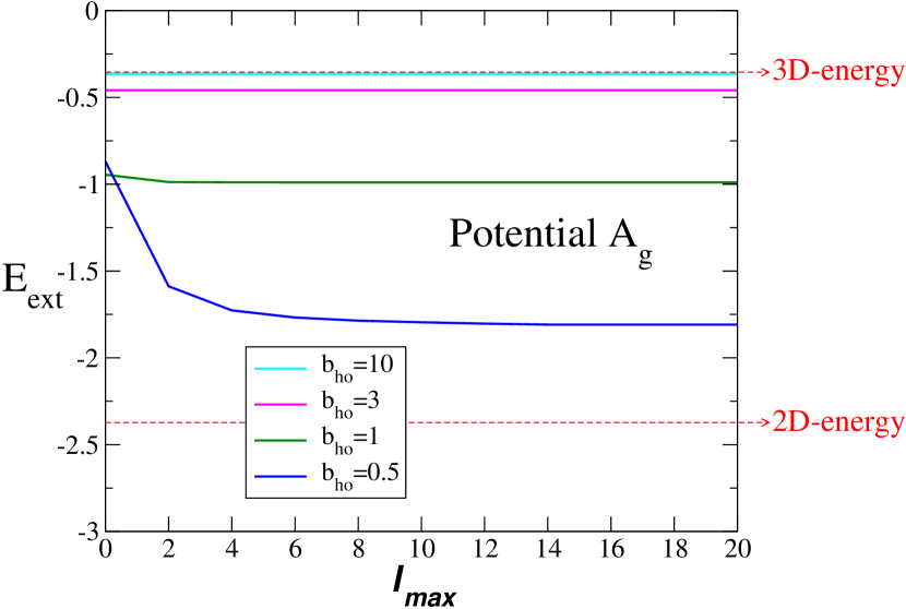
Figure 1: For the Gaussian potential A_g and an external squeezing harmonic oscillator field, we show the three-body ground state binding energy, $E_{ext}=E_{3b}-E_{ho}$, as a function of the maximum $\ell_{y}$-value, $\ell_{max}$, used on each Jacobi set. The results with different values of the squeezing parameter $b_{ho}$ are shown. The lower and higher horizontal dashed lines indicate the 2D and 3D energies, respectively. The energy is in units of $\hbar^{2}/mb^{2}$, where $m$ is the mass of each particle and $b$ is the range of the interaction.

However, this method presents two main problems. The first one refers to the fact that, as seen in Eq.(27), although $\ell_{x}$ (taken equal to zero in this work) is conserved all along the squeezing process, the orbital angular momentum $\ell_{y}$, and therefore $L$ as well, are not good quantum numbers anymore. This mixing of partial waves is introduced by the squeezing potential, and in fact, the larger the squeezing of the particles the more partial waves are needed.

This is illustrated in Fig.1, where we show for the Gaussian potential A_g in Table 1 how the ground state energy, $E_{ext}=E_{3b}-E_{ho}$, of the confined three-body system converges as a function of $\ell_{max}$, where $\ell_{max}$ refers to the maximum value of $\ell_{y}=L$ included on each of the Faddeev components. The lower and higher horizontal dashed lines in the figure indicate the ground state energy after a pure 2D and a pure 3D calculation, respectively. The results are shown for different values of the squeezing parameter $b_{ho}$.

As we can see, for sufficiently large values of $b_{ho}$ the convergence is very fast and just a few $\ell_{y}$ components, very often only one, are enough. Eventually, for very large $b_{ho}$ the 3D energy is recovered. With decreasing $b_{ho}$ we observe that higher and higher values of $\ell_{max}$ are needed. For instance, for $b_{ho}=0.5$ the components with $\ell_{y}$ up to at least 14 are necessary to get convergence. For a sufficiently small value of $b_{ho}$ the converged energy should eventually match the 2D-energy indicated by the lower dashed straight line in the figure.

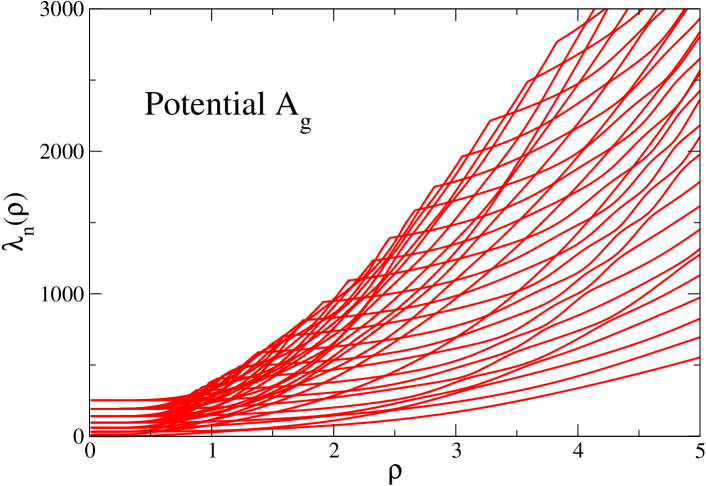
Figure 2: Thirty lowest $\lambda_{n}$-functions for potential A_g, squeezing external harmonic oscillator field with oscillator length $b_{ho}=0.2$, and $\ell_{max}=14$.

However, to get the same kind of curve for smaller values of $b_{ho}$ is not simple. This is due to the second problem to be faced when solving the three-body equations with an external potential, which refers to the convergence of the expansion in Eq.(16). The number of terms needed for convergence increases with the confinement of the particles. This should not be a big problem in itself, except for the fact that when the squeezing of the particles increases (small $b_{ho}$-values), the number of crossings between the different $\lambda_{n}$-functions entering in Eq.(8) becomes eventually too high, which increases dramatically the computing time. This problem is actually enhanced by the fact that, as explained above, the number of required partial waves increases as well with the confinement.

As an illustration we show in Fig. 2 the 30 lowest $\lambda_{n}(\rho)$ functions for potential A_g, $b_{ho}=0.2$, and $\ell_{max}=14$. To deal with such a huge number of crossings is very much time consuming, and makes this method rather inefficient close to 2D. Towards this limit the method of correlated gaussians moe19 might for example be used, although the advantage of very similar basis functions would then also disappear. The choice is then between using different methods in the two limits or the same method with inherent loss of efficiency in one of the limits.

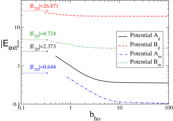
Figure 3: For the case of squeezing with an external harmonic oscillator field, absolute value of the converged three-body ground state energies (in units of $\hbar^{2}/mb^{2}$) for the Gaussian potentials A_g (solid) and B_g (dashed), and the Morse potentials A_m (dot-dashed) and B_m (dot), as a function of $b_{ho}$ (in units of the range of the interaction). The arrows indicate the 2D energy that should be reached for $b_{ho}=0$.

The conclusion is therefore that to include explicitly the external potential as described in Section III.1 is not very convenient in the case of large squeezing. To reach convergence for low values of the squeezing parameter becomes at some point too troublesome. In Fig.3 we show the computed converged energies of the three-body ground state for the four potentials given in Table 1 as a function of $b_{ho}$. In the limit of $b_{ho}=0$ the 2D energies indicated by the arrows in the figure should be reached.

VIII Results: The $d$-calculation

Pot.	$E_{2D}$	$r_{2D}$	$E_{3D}$	$r_{3D}$
Ag	$-2.373$	0.591	$-0.354$	1.081
	$-0.556$	3.339	$-6.109\cdot 10^{-3}$	10.280
Bg	$-26.871$	0.304	$-19.426$	0.390
	$-14.622$	0.518	$-9.050$	0.632
	$-7.990$	1.678
Am	$-0.644$	1.145	$-0.104$	2.201
	$-0.160$	4.695	$-4.808\cdot 10^{-3}$	15.744
Bm	$-4.724$	0.613	$-2.834$	0.848
	$-2.202$	1.220	$-1.087$	1.628

Table 2: For $d=2$ and $d=3$, we give the three-body energies and root-mean square radii, $r=\langle\rho^{2}/3\rangle^{1/2}$, for all the bound states obtained with the potentials given in Table 1. The subscripts $2D$ and $3D$ refer to the results obtained for $d=2$ and $d=3$, respectively. As done all along the text, the energies are given in units of $\hbar^{2}/mb^{2}$, where $m$ is the mass of each of the particles (and the normalization mass used to construct the Jacobi coordinates), and $b$ is the range of the two-body interaction, which is taken as length unit.

To perform the three-body calculations as described in Section II, where the external potential does not enter and the dimension $d$ is treated as a parameter, is certainly much simpler than the calculations shown in the previous section. In Table 2 we give the computed energies and root-mean-square (rms) radii in two and three dimensions for all the three-body bound states obtained after solving the coupled Eqs.(8) with the two-body potentials given in Table 1. The energies, $E_{2D}$ and $E_{3D}$, and the rms values, $r_{2D}$ and $r_{3D}$, refer to the results obtained with $d=2$ and $d=3$, respectively. As we can see, whereas potentials A_g, A_m, and B_m have the same number, two, of bound three-body states in 3D as in 2D, potential B_g has one bound state less in 3D, two, than in 2D, three.

In Fig. 4 we show the absolute value of the bound three-body energies obtained with potentials A_g, B_g, A_m, and B_m (panels (a), (b), (c), and (d), respectively) as a function of $(d-2)/(3-d)$, where $d$ is the dimension running within the range $2\leq d\leq 3$. The choice of the abscissa coordinate as $(d-2)/(3-d)$ has been made to facilitate the comparison with Fig. 3, since in both figures values of the abscissa coordinate equal to zero and infinity correspond, respectively, to maximum squeezing of the system into 2D and no squeezing (3D). In the figure the dotted (blue) curve shows, for each of the potentials and also as a function of $(d-2)/(3-d)$, the absolute value of the lowest two-body bound state energy.

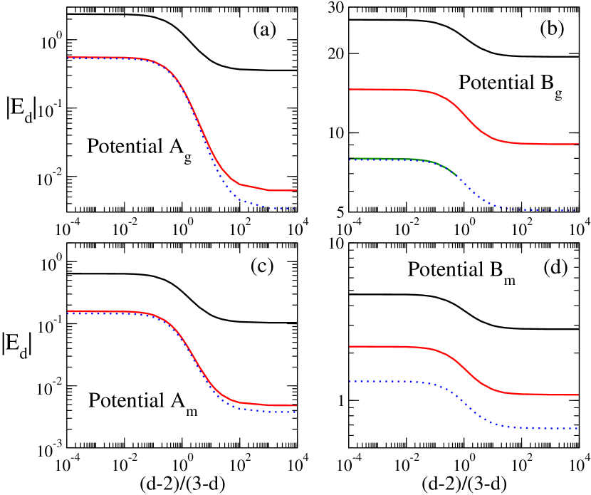
Figure 4: With the $d$-method, absolute value of the bound state three-body energies obtained with potentials A_g, B_g, A_m, and B_m in Table 1 (panels (a), (b), (c), and (d), respectively) as a function of $(d-2)/(3-d)$ where $d$ runs within the range $2\leq d\leq 3$. For each of the potentials, the dotted blue curve is the absolute value of the lowest bound two-body state energy.

As a general rule, when squeezing from $d=3$ to $d=2$ the three-body system becomes progressively more and more bound. This is clearly seen for all the potentials when moving from the right part on each panel ($d=3$) to the left part ($d=2$). This is a reflection of the lower centrifugal barrier in 2D than in 3D.

In the case of potentials A_g and A_m, Figs. 4a and 4c, the curve corresponding to the excited three-body bound state (red curve) approaches the dotted curve representing the bound two-body energy. In fact, very soon the three-body excited state is just slightly more bound than the two-body state, representing therefore a boson very weakly bound with respect to the two-body bound state.

For potential B_g, Fig. 4b, a new bound state shows up for $d\approx 2.4$. It appears from the threshold corresponding to the bound two-body state and the third boson. From that point and up to $d=2$ the third three-body bound state follows closely the two-body binding energy (dotted curve). Thus, as for potentials A, the last excited state corresponds to a very weakly bound boson with respect to the two-body bound state.

For potential B_m the situation seems to be different compared to the other potentials, since in this case there is no three-body bound state approaching the two-body bound state curve (dotted curve). However, the behavior of the three-body spectrum for this potential is actually very similar to the one of potential B_g in Fig. 4b. The only difference is that the dimension at which the third bound state appears from the two-body threshold is $d\approx 1.9$, lying therefore out of the graph limits. It would certainly be possible to extend the investigation to confinement scenarios up to dimensions smaller than 2, eventually up to $d=1$ or even smaller, but this is left for a future work.

IX Wave functions

In Section IV the relation between the harmonic oscillator parameter, $b_{ho}$, and the dimension, $d$, was discussed. In particular, the relation in Eq.(32) was found for the simple case where the particle-particle interaction is assumed to be a harmonic oscillator potential with length parameter $b_{pp}$. This length, $b_{pp}$, is also the root-mean-square radius of the three-body system in 3D, whereas in 2D the root-mean-square radius is $r_{2D}=b_{pp}\sqrt{2/3}$, which permits to rewrite Eq.(32) as:

$$\frac{b_{ho}}{r_{2D}}=\sqrt{\frac{3(d-2)}{(d-1)(3-d)}}.$$ (47)

Instead of this simple expression, the full numerical solution from the Gaussian and Morse short-range interactions can be found, and the energies compared. In the same way that Eq.(32) has been obtained by making equal $E_{d}$ and $E_{ext}$ in Eqs.(29) and (IV), we can use Fig. 3 and Fig. 4 to obtain numerically the relation between $d$ and $b_{ho}$, at least for the $b_{ho}$-values for which, as shown in Fig. 3, the energy $E_{ext}$ can be obtained.

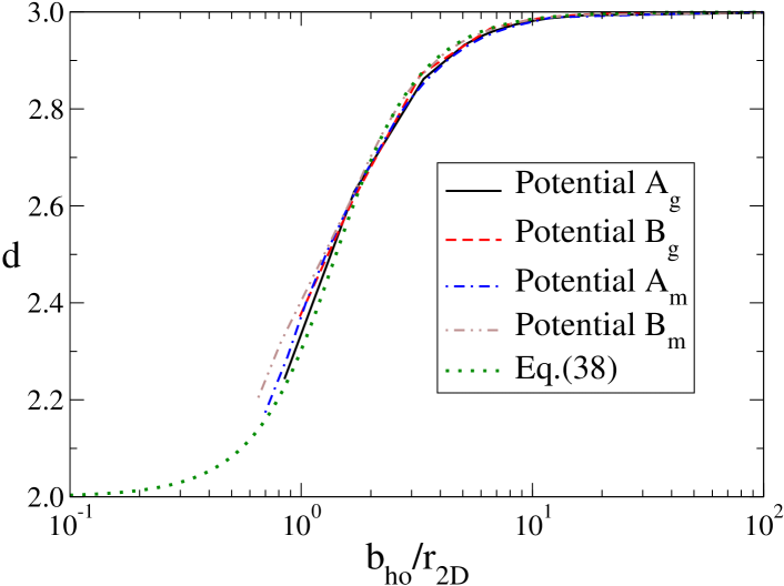
Figure 5: Numerical relation between the dimension $d$ and the harmonic oscillator parameter $b_{ho}$ obtained after making equal $E_{ext}$ in Fig. 3 and the ground state energy $E_{d}$ in Fig. 4. The oscillator parameter $b_{ho}$ is normalized to the root-mean-square radius of the 2D three-body calculation. The cases of potentials A_g, B_g, A_m, and B_m are shown by the solid, dashed, dot-dashed, and dot-dot-dashed curves ,respectively. These results are compared with the estimate given in Eq.(47), which is shown by the dotted curve.

The results are shown in Fig. 5 by the solid, dashed, dot-dashed, and dot-dot-dashed curves for potentials A_g, B_g, A_m, and B_m, respectively. They have been obtained using the energies of the three-body ground state. The numerical curves are compared with the analytical expression given by Eq.(47), which is shown by the dotted curve.

As we can see, the estimate in Eq.(47) agrees reasonably well with the calculations in those regions where the numerical calculation with the external potential has been possible. This is especially true for potentials A_g, B_g, and A_m, whereas for potential B_m a somewhat bigger discrepancy is observed for large squeezing. In any case, for those small values of the squeezing parameter, $b_{ho}$, the complications inherent to the numerical calculations with the external potential can be a source of inaccuracy for $E_{ext}$. Furthermore, since $b_{ho}=0$ must necessarily correspond to $d=2$, we can consider the expression (47) a reliable translation to the parameter, $d$, in relatively easy calculations from a given small value of the squeezing parameter, $b_{ho}$.

As shown in Section V, the equivalence between the three-body wave functions with the two calculations can be directly compared through the overlap in Eq.(41), where $\Psi_{ext}$ is the wave function obtained with the external squeezing potential, and $\tilde{\Psi}_{d}$ is the one obtained with the $d$ calculation after the transformation in Eqs.(38) and (39), and the subsequent renormalization. Obviously, the values of $b_{ho}$ and $d$ have to be such that they both give rise to the same ground state three-body energy. As discussed in Section V, this overlap permits to extract the scale parameter, $s$, in the transformation in Eqs.(38) and (39) as the value that maximizes the overlap.

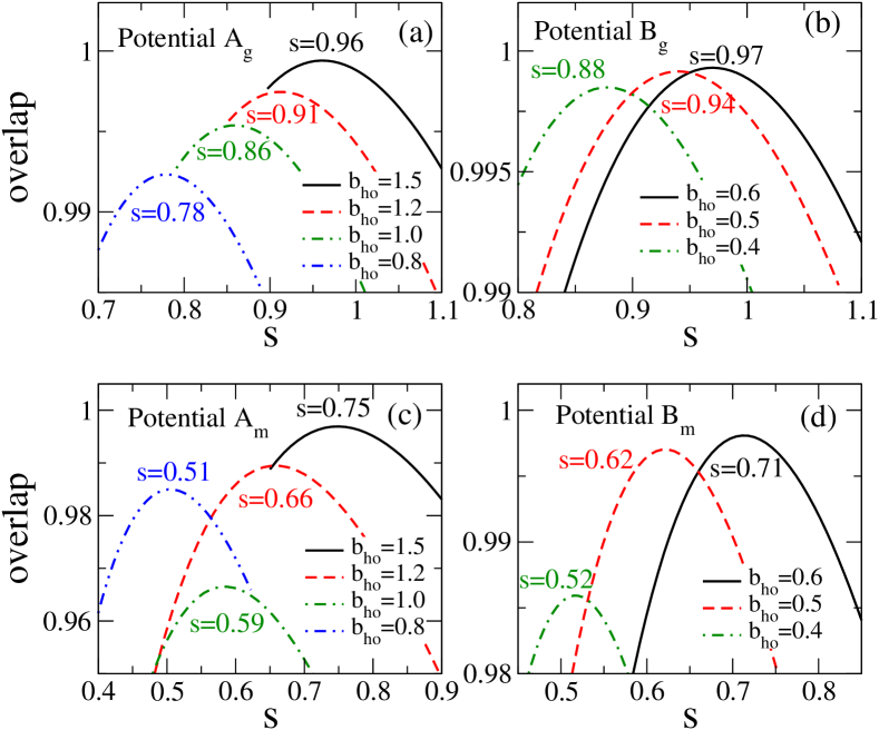
Figure 6: Overlap ${\cal O}(s)$ as a function of the scale parameter $s$ for potentials A_g, B_g, A_m, and B_m (panels (a), (b), (c), and (d), respectively) and different values of the external potential parameter $b_{ho}$. For each $b_{ho}$ the dimension $d$ is the one giving rise to the same ground state binding energy. For each case we indicate the value of $s$ corresponding to the maximum overlap.

In Fig. 6 we show the overlap ${\cal O}(s)$ as a function of the scale parameter, $s$, for the the four potentials considered in this work. Several different values of the squeezing parameter, $b_{ho}$, have been chosen, and for each of them we determine, according to Fig. 5, the value of the dimension, $d$, giving rise to the same ground state binding energy. As seen in Fig. 6, in all the cases the curves show a well defined maximum, which determine the value of the scale parameter, $s$, to be used in the $d$-function $\tilde{\Psi}_{d}$.

$b_{ho}$	Pot. Ag		Pot. Bg		Pot. Am		Pot. Bm
	$s$	$d$	$s$	$d$	$s$	$d$	$s$	$d$
0.4			0.88	2.489			0.52	2.205
0.5			0.94	2.604			0.62	2.318
0.6			0.97	2.694			0.71	2.383
0.8	0.78	2.523			0.51	2.173
1.0	0.86	2.628			0.59	2.289
1.2	0.91	2.704			0.66	2.400
1.5	0.96	2.783			0.75	2.511

Table 3: For each of the potentials and each of the selected values of $b_{ho}$ shown in Fig.6, we give the corresponding values of the scale parameter $s$ that maximizes the overlap in Eq.(41) and the dimension $d$ giving rise to the same ground state binding energy.

Fig. 6a shows the results for potential A_g. As we can see, for $b_{ho}=1.5$, which corresponds to $d=2.783$, we obtain a scale parameter of $s=0.96$, which indicates that the deformation of the $d$-calculated wave function produced by the squeezing is in this case rather modest. For larger squeezing (smaller values of $b_{ho}$), the scale parameter starts decreasing, reaching the values of $s=0.91$, $s=0.86$, and $s=0.78$ for $b_{ho}=1.2$ ($d=2.704$), $b_{ho}=1.0$ ($d=2.628)$, and $b_{ho}=0.8$ ($d=2.523$), respectively. These results are collected in the second column of Table 3.

The deformation of the $d$-calculated wave function produced by a given squeezing is very sensitive to the size of the three-body system. For instance, as seen in Table 2, for potential B_g the ground state in 3D is about three times smaller than the one for potential A_g. For this reason one can intuitively think that a larger squeezing (smaller $b_{ho}$) will be necessary in order to get a similar deformation of the wave function. This is actually seen in Fig. 6b, where the overlap ${\cal O}(s)$ for potential B_g is shown (the corresponding $s$ and $d$ values are given in the third column of Table 3). As we can see, even for a squeezing parameter $b_{ho}=0.6$ ($d=2.694$) the scale parameter is still not too far from 1, whereas for $b_{ho}=0.5$ ($d=2.604$) and $b_{ho}=0.4$ ($d=2.489$) the corresponding values of $s$ are similar to the ones obtained for potential A_g (Fig.6a) when $b_{ho}=1.2$ and $b_{ho}=1.0$, respectively.

In Figs. 6c and 6d we show the same results for the Morse-like potentials A_m and B_m, respectively, and the values of $s$ and $d$ are also given in the fourth and fifth columns of Table 3. The general behavior is similar to the one found for the Gaussian potentials. The three-body system is again about three times bigger in 3D with potential A_m than with potential B_m. The result is therefore that similar deformation, i.e. similar values of the scale parameter $s$, requires less squeezing, larger value of $b_{ho}$, with potential A_m than with potential B_m. The same happens when comparing potentials A_m with A_g, and B_m with B_g. Since the Morse 3D states are clearly bigger than the corresponding Gaussian counterparts, we again find that for equal values of $b_{ho}$ the bigger systems, the ones obtained with potentials A_m and B_m, are more deformed (smaller value of $s$) than with potentials A_g and B_g, respectively.

The maximum overlap shown in Fig. 6 is always very close to 1, always above 0.96, but typically around 0.98 or even higher. This indicates that the deformation described by Eqs.(38) and (39) works in general very well, although for some of the cases, like for instance potential A_m with $b_{ho}=1.0$ (where the maximum overlap is about 0.96), a correction could probably be introduced.

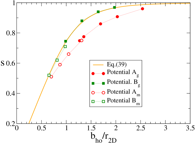
Figure 7: Scale parameter $s$ as a function of $b_{ho}/r_{2D}$ for the four potentials used in this work. The solid curve shows the estimate given in Eq.(48).

The values of the computed scale parameters are shown in Fig. 7 as a function of $b_{ho}/r_{2D}$. Together with them we show the estimate given in Eq.(46). More precisely, exploiting again the fact that in the case of the harmonic oscillator two-body potential we have that $b_{pp}=r_{2D}\sqrt{3/2}$, we can then rewrite Eq.(46) as:

$$\frac{1}{s^{2}}=\sqrt{1+\frac{9}{4}\left(\frac{r_{2D}}{b_{ho}}\right)^{4}},$$ (48)

which is shown in Fig. 7 by the solid curve. As we can see, the estimate given above works very well for potentials B_g and B_m (squares in the figure), which correspond to the cases of well bound three-body states in 3D (Table 2). In fact, for potential B_g, for which $|E_{3D}|$ is pretty large, the agreement is excellent. For the cases when the system is clearly less bound in 3D, potentials A_g and A_m (circles in the figure), the computed results disagree with the estimate in Eq.(48) in the region of intermediate squeezing. However, it is interesting to see how, for large squeezing, the computed curve for potentials A_g and A_m and the solid curve clearly converge. Therefore the estimate (48) appears as a very good way of determining the equivalence between $s$ and $b_{ho}$ also for potentials A_g and A_m in the cases of large squeezing, which, on the other hand, are the cases where the calculations with the external potential are more problematic.

Finally, let us directly compare the wave functions $\Psi_{ext}$ and $\tilde{\Psi}_{d}$. This can be done by simple comparison of the radial wave functions contained in the expansions Eqs.(16) and (42). Since the angular functions are the same in the two cases, the difference between the two wave functions will be necessarily contained in the radial functions $f_{n}(\rho)$ and $\tilde{f}_{n}^{(d)}(\rho,s)$.

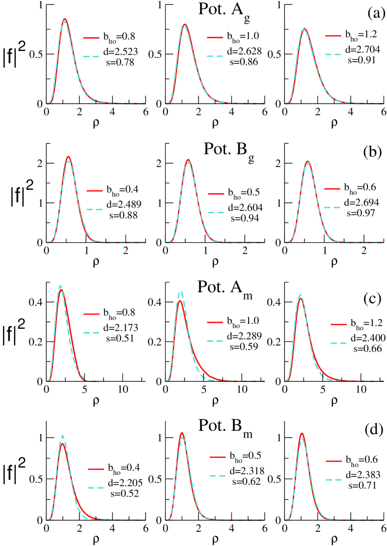
Figure 8: The solid curves show, as a function of $\rho$, the square of the dominating radial wave functions, $f_{n}(\rho)$ in Eq.(16), for the potentials and external field parameters $b_{ho}$ shown in Fig. 6 (except the cases with $b_{ho}=1.5$, which, for simplicity in the figure, have been omitted). Panels (a), (b), (c), and (d) correspond to potentials A_g, B_g, A_m, and B_m, respectively. For each case, the dashed curve gives, also as a function of $\rho$, the square of the radial wave function $\tilde{f}_{n}^{(d)}(\rho,s)$ shown in Eq.(43), where the dimension $d$ provides the same ground state energy as the calculation with the external field, and the scale parameter $s$, given in Fig. 6, maximizes the overlap ${\cal O}(s)$ in Eq.(41). The length unit is the range of the two-body interaction.

In Fig. 8 we show the squares of the dominating radial wave functions, $f_{n}(\rho)$ (solid curves) and $\tilde{f}_{n}^{(d)}(\rho,s)$ (dashed curves), for some of the cases shown in Fig. 6 (in order to make the figure simpler the cases with $b_{ho}=1.5$ have been omitted). In all of them, the dominating term provides more than 98% of the total norm. Panels (a), (b),(c), and (d) correspond to the results with potentials A_g, B_g, A_m, and B_m, respectively. The values of the dimension, $d$, and the scale parameter, $s$, are as indicated in Table 3, i.e. the dimension, $d$, is such that the $d$-calculation gives the same ground state energy as in the calculation with the external squeezing potential, and the scale parameter, $s$, is such that the overlap, ${\cal O}(s)$, in Eq.(41), is maximum.

As we can see in the figure the agreement is very good basically for all the cases shown. The largest discrepancy is observed for Morse potential A_m with $b_{ho}=1.0$, which, as seen in Fig. 6, is the case with the smallest value of the maximum overlap, below 0.97, between the two wave functions. In any case, the good agreement between the two radial wave functions illustrates how the wave function resulting from the $d$-calculation, after the appropriate reinterpretation in the ordinary 3D space, provides a very good description of the system squeezed by an external potential.

X Summary and conclusions

In this work the continuous squeezing of three-body systems from 3 to 2 dimensions has been investigated by means of two different procedures: First, a method where the external confining potential is explicitly included, and second, a method where the external potential does not enter, but instead, the dimension $d$ is allowed to take any intermediate value between $d=3$ and $d=2$.

The case of three identical spinless bosons with relative $s$-waves between all the particles is considered. For the two-body potentials we have used Gaussian and Morse radial forms whose scattering length vary from small, with a few fairly well bound states, to rather large.

For the three-body calculations with an external field we have chosen the squeezing potential to be a one-body deformed harmonic oscillator acting on each of the three particles. The oscillator length in one of the dimensions is varied from infinity (no squeezing) to a very small value corresponding to a fraction of the two-body interaction range. The deformation produced by the squeezing breaks orbital angular momentum conservation, and the calculations must account for the resulting mixing of these quantum numbers. The consequence is that the adiabatic hyperspherical expansion must employ a large number of partial wave components in the limit where the dimension $2$ is approached.

The method with the non-integer dimension, $d$, as parameter is formulated in terms of hyperspherical coordinates with spherical potentials and $s$-waves. The phase space and centrifugal barrier potentials both correspond to the specified value of $d$. This method is technically precisely as simple as the ordinary three-body three-dimensional computations without external field.

With the two methods we have investigated how the ground state energies vary when squeezing from three to two dimensions. Both methods show the same qualitative behavior although the connection between the 2D and 3D limits must be different in the two cases, since the oscillator length of the external potential and the dimension, $d$, vary in infinite and finite intervals, respectively. The three-body bound states do not necessarily have counterparts in the 3D and the 2D limits.

Comparison of the results from the two methods allows extraction of the function translating between $d$ and the oscillator length of the external squeezing potential. The knowledge of this function provides a subsequent prediction of which external field corresponds to a given $d$-value. To give us some insight, we have used a simplified system where harmonic oscillators (different to the external field) are used for the two-body interactions. We have in this way obtained an analytic expression relating the dimension $d$ and the oscillator length of the external field. This estimate is then compared to the results arising from the numerical computations. By choosing the root-mean-square radius of the three-body system in two dimensions as length unit, we have found that the translational functions are remarkably similar to each other, as well as to the analytic function derived for the two-body oscillator potential.

To be able to predict any observable property entirely from $d$-calculations, we must also find a translation or interpretation providing the wave function corresponding to a three dimensional calculation with an external field. We naturally search for a deformed solution obtained from the spherical wave function in the $d$-method. This is achieved by scaling the squeezing coordinate relative to the two other coordinates. The scaling factor must depend on $d$, and it is defined such that the overlap between the two wave functions of equal energy from the two methods is maximum, preferentially unity.

This interpretation of the $d$-calculated wave function is suggested by the exact solution available when using oscillator interactions between the particles as well as for the external field. This analytic approximation is compared to the scaling parameter extracted numerically. The computed values are surprisingly close to the analytic curve for the potentials with well bound three-body states in 3D, whereas they deviate when the three-body system is weakly bound in three dimensions. Comparing directly the wave functions from the two methods we find a remarkable agreement between them.

In summary, we have in details investigated a new method to deal with three-body problems in non-integer dimensions between $2$ and $3$. The basis is a $d$-dimensional phase space, a corresponding $d$-dependent generalized centrifugal barrier, and a spherical computation. The calculations are precisely as simple as the same three-body calculations in integer dimensions. We validate the method by comparing to the brute force method in the ordinary three-dimensional space. The non-integer dimension is simulated by a deformed external field, which effectively reduces movement in one coordinate from being free (in 3D) to zero space (in 2D).

The equivalence of the two methods is shown for identical bosons by numerical calculations, where we provide a relatively accurate translation between the parameter $d$ and the external field length. This connection includes a prescription to obtain the complete deformed wave function from the $d$-calculation. Since the translation correctly reproduces the two limits of 2D and 3D, any prediction occurring for some $d$-value is bound to happen for some external field strength, which in turn is relatively precisely given by an analytic expression.

The presented $d$-method can be extended to asymmetric three-body systems with different mass ratios, to dimensions smaller than 2 and larger than 3, and perhaps to fermions and particle numbers larger than three.

Appendix A $s$-wave spherical and hyperspherical harmonics in $d$ dimensions

The angle independent $s$-wave spherical harmonic in $d$ dimensions, $Y_{0}$, can be obtained by taking into account that the phase volume in $d$ dimensions is given by hay01 :

$$\int d\Omega_{d}=\frac{2\pi^{d/2}}{\Gamma\left(\frac{d}{2}\right)},$$ (49)

from which, since $\int Y_{0}^{*}Y_{0}d\Omega_{d}=1$, one immediately gets:

$$Y_{0}=\left[\frac{\Gamma\left(\frac{d}{2}\right)}{2\pi^{d/2}}\right]^{1/2}.$$ (50)

Thus, the angular functions, $\Phi_{n}^{(d,i)}$, in Eq.(7) depend only on the hyperangle $\alpha=\arctan(x/y)$, where $\bm{x}$ and $\bm{y}$ are the usual Jacobi coordinates nie01 . Typically, these angular functions are obtained as an expansion in terms of the hyperspherical harmonics, which for $d$ dimensions and relative $s$-waves, take the form nie01 :

$${\cal Y}_{K}^{(d)}(\alpha)=N_{\nu}P_{\nu}^{\left(\frac{d-2}{2},\frac{d-2}{2}\right)}(\cos 2\alpha)Y_{0}Y_{0},$$ (51)

where $K=2\nu$ is the hypermomentum, $N_{\nu}$ is the normalization constant, and $P_{\nu}^{\left(\frac{d-2}{2},\frac{d-2}{2}\right)}$ is a Jacobi polynomial.

Finally, when solving the three-body problem it is always necessary at some point to rotate the hyperspherical harmonics (51) from one Jacobi set $i$ into a different set $j$. This is done by means of the Raynal-Revai coefficients, which for $s$-waves and $d$ dimensions are given by nie01 :

$$\langle{\cal Y}_{K}(i)|{\cal Y}_{K^{\prime}}(j)\rangle=\delta_{KK^{\prime}}\frac{P_{\nu}^{\left(\frac{d-2}{2},\frac{d-2}{2}\right)}(\cos 2\gamma_{ij})}{P_{\nu}^{\left(\frac{d-2}{2},\frac{d-2}{2}\right)}(1)},$$ (52)

where the angle $\gamma_{ij}$ is given for instance in Ref.nie01 .

References

- (1) I. Bloch, J. Dalibard, and W. Zwerger, Rev. Mod. Phys. 80, 885 (2008).
- (2) S. Deng, Z.-Y. Shi, P. Diao, Q. Yu, H. Zhai, R. Qi, and H. Wu, Science 353, 371 (2016).
- (3) J.R. Armstrong, A.G. Volosniev, D.V. Fedorov, A.S. Jensen, and N.T. Zinner, J. Phys. A: Math. Theor. 48, 085301 (2015).
- (4) F. S. Møller, D. V. Fedorov, A. S. Jensen, N. T. Zinner, J. Phys. B: At. Mol. Opt. Phys. 52, 145102 (2019).
- (5) M.T. Yamashita, F.F. Bellotti, T. Frederico, D.V. Fedorov, A.S. Jensen, N. T. Zinner, J. Phys. B: At. Mol. Opt. Phys. 48, 025302 (2015).
- (6) J.H. Sandoval, F.F. Bellotti, A.S. Jensen, and M.T. Yamashita, J. Phys. B: At. Mol. Opt. Phys. 51, 065004 (2018).
- (7) D.S. Rosa, T. Frederico, G. Krein, and M.T. Yamashita, Phys. Rev. A 97, 050701(R) (2018).
- (8) J. Levinsen, P. Massignan, and M.M. Parish, Phys. Rev. X 4, 031020 (2014).
- (9) E. Garrido, A.S. Jensen, and R. Álvarez-Rodríguez, Phys. Lett. A 383, 2021 (2019).
- (10) E. Garrido and A.S. Jensen, Phys. Rev. Research 1, 023009 (2019).
- (11) E. Nielsen, D.V. Fedorov, A.S. Jensen, and E. Garrido, Phys. Rep. 347, 373 (2001).
- (12) A.S. Jensen, K. Riisager, D.V. Fedorov, and E. Garrido, Rev. Mod. Phys. 76, 215 (2004).
- (13) E. Garrido, Few-Body Syst. 59, 17 (2018).
- (14) S.I. Hayek, Advanced Mathematical Methods in Science and Engineering, Marcel Dekker Inc., (2001) p.645.