Proof of Laugwitz Conjecture and Landsberg Unicorn Conjecture for Minkowski norms with $SO(k)\times SO(n-k)$-symmetry.

Abstract.

For a smooth strongly convex Minkowski norm $F:\mathbb{R}^{n}\to\mathbb{R}_{\geq 0}$, we study isometries of the Hessian metric corresponding to the function $E=\tfrac{1}{2}F^{2}$. Under the additional assumption that $F$ is invariant with respect to the standard action of $SO(k)\times SO(n-k)$, we prove a conjecture of Laugwitz stated in 1965. Further, we describe all isometries between such Hessian metrics, and prove Landsberg Unicorn Conjecture for Finsler manifolds of dimension $n\geq 3$ such that at every point the corresponding Minkowski norm has a linear $SO(k)\times SO(n-k)$-symmetry.

Mathematics Subject Classification (2010): 52A20, 53C21, 53C30, 53B40.

Key words: Minkowski norm, Hessian isometry, Laugwitz Conjecture, Landsberg Unicorn Conjecture, Legendre transformation

1. Introduction

1.1. Definitions and state of the art

For a (smooth) function $E(x_{1},...,x_{n})$, the Hessian ${\rm d}^{2}E=\left(\frac{\partial^{2}E}{\partial x_{i}\partial x_{j}}\right)$ is a symmetric bilinear form. If it is positive definite, it defines a Riemannian metric called the Hessian metric. Though the construction strongly depends on the coordinate system, Hessian metrics naturally appear in many subjects of mathematics.

For example, for toric Kähler manifolds, the metrics on the quotient space are (locally) Hessian metrics. Metrics admitting nontrivial geodesic equivalence are also Hessian metrics, see e.g. [12, §4.2]. There is a strong relation between Hessian metrics and the Hamiltonian construction in the theory of infinite-dimensional integrable system of hydrodynamic type, see e.g. [23]. Hessian metrics naturally come in many geometric constructions of Riemannian metrics inside convex domains (see e.g. [15]), in affine geometry of hypersurfaces (see e.g. [29, 30]) and in information geometry (see e.g. [42]). We refer to [41] for a comprehensive study of differential geometry of Hessian metrics and their applications.

We are interested in Hessian metrics that naturally appear in convex and Finsler geometry. They are defined on $\mathbb{R}^{n}\setminus{\{0\}}$ and the function $E$ satisfies the following restriction: it is positively 2-homogeneous, that is, for any $\lambda{\geq 0}$ we have $E(\lambda y)=\lambda^{2}E(y)$.

Under this assumption, the property that ${\rm d}^{2}E$ is positive definite is equivalent to the condition that $E$ is positive on $\mathbb{R}^{n}\setminus\{0\}$ and that $F:=\sqrt{2E}$ satisfies the following properties: it is positively 1-homogeneous (i.e., $F(\lambda y)=\lambda F(y)$ for $\lambda\geq 0$), convex (i.e. $F(y_{1}+y_{2})\leq F(y_{1})+F(y_{2})$) and strongly convex (i.e., the second fundamental form of the indicatrix $S_{F}:=\{y\in\mathbb{R}^{n}\mid F(y)=1\}$ is positive definite). Functions $F$ with such properties are called Minkowski norms. All Minkowki norms we consider below are smooth and strongly convex.

It is known that the indicatrix $S_{F}$ determines the Minkowski norm $F$ and (as we recall below) that the Hessian metric of $E=\tfrac{1}{2}F^{2}$ determines the function $E$. So the study of strongly convex bodies with smooth boundary can be reduced to the study of Hessian metrics for $E=\tfrac{1}{2}F^{2}$ and in particular apply methods and results of Riemannian geometry. We refer to [29, 40] for more details on the interrelation between Hessian geometry and convex geometry. In later discussion, we will reserve the notation $F$ for the Minkowski norm and $E=\frac{1}{2}F^{2}$ for the function we use to build a Hessian metric.

The appearance of Hessian metrics in Finsler geometry is related to that in the convex geometry. Recall that a Finsler metric on a smooth manifold $M$ with $\operatorname{dim}M>1$ is a continuous function $F$ on $TM$ such that it is smooth on the slit tangent bundle $TM\setminus\{0\}$ and such that its restriction to each tangent space $T_{p}M$ is a Minkowski norm. The corresponding Hessian metric $g$ is then a Riemannian metric on the slit tangent space $T_{p}M\setminus\{0\}$. It was called the fundamental tensor by L. Berwald [9] and it naturally comes to many geometric constructions in Finsler geometry.

In this paper we study isometries between the Hessian metrics of Minkowski norms. We call the diffeomorphism $\Phi:\mathbb{R}^{n}\backslash\{0\}\rightarrow\mathbb{R}^{n}\backslash\{0\}$ a Hessian isometry from $F_{1}$ to $F_{2}$, if it is an isometry between the Hessian metrics $g_{1}={\rm d}^{2}E_{1}=\tfrac{1}{2}{\rm d}^{2}(F_{1}^{2})$ and $g_{2}={\rm d}^{2}E_{2}=\tfrac{1}{2}{\rm d}^{2}(F_{2}^{2})$. By local Hessian isometry we understand a positively 1-homogeneous diffeomorphism between two conic domains that is isometry with respect to the restriction of the Hessian metrics to these domains. Here the positive 1-homogeneity for the local Hassian isometry $\Phi$ is the property that $\Phi(\lambda x)=\lambda\Phi(x)$ for any $\lambda>0$ and any $x\in\mathbb{R}^{n}\backslash\{0\}$ where $\Phi$ is defined. By conic domain we understand

$$C(U):=\{\lambda y\ \mid\ y\in U\ ,\ \lambda>0\},\textrm{\ where $U\subset\mathbb{R}^{n}\backslash\{0\}$}.$$

Let us recall some known facts (e.g. [8, 29]) that follow from the positive 1-homogeneity of $F$.

• The Hessian metric determines geometrically the “radial” rays, i.e., the sets of the form $\{ty\mid t\in\mathbb{R}_{>0}\}$, with nonzero $y$. Indeed, these rays are geodesics for the Hessian metrics, and are precisely those which are not complete.

• The Hessian metric $g=\tfrac{1}{2}{\rm d}^{2}E$ determines the functions $E$ and $F$ by $F(y)^{2}=g(y,y)$ for every $y\in\mathbb{R}^{n}\backslash\{0\}$.

• The Hessian metric $g$ is the cone metric over its restriction to the indicatrix $S_{F}$, i.e., $g=({\rm d}F)^{2}+F^{2}g_{|S_{F}}$. That is, in any local coordinate system $(r,\xi_{2},...,\xi_{n})$ such that $F(r,\xi_{2},...,\xi_{n})=r$, we have $g=dr^{2}+r^{2}\sum_{i,j=2}^{n}h_{ij}d\xi_{i}d\xi_{j}$, where the components $h_{ij}$ do not depend on $r$.

These three observations imply that any Hessian isometry $\Phi$ from $F_{1}$ to $F_{2}$ satisfies the positive 1-homogeneity and diffeomorphically maps the indicatrix $S_{F_{1}}$ to $S_{F_{2}}$. Any local Hessian isometry $\Phi:C(U_{1})\to C(U_{2})$ is 1-homogeneous by definition and diffeomorphically maps $S_{F_{1}}\cap C(U_{1})$ to $S_{F_{2}}\cap C(U_{2})$.

Moreover, a positively 1-homogeneous mapping $\Phi$ which maps $S_{F_{1}}$ to $S_{F_{2}}$ is a Hessian isometry if an only if its restriction to $S_{F_{1}}$ an isometry between ${g_{i}}_{|S_{F_{i}}}$.

Let us now recall some known examples of Hessian isometries.

If $\Phi:\mathbb{R}^{n}\to\mathbb{R}^{n}$ is a linear isomorphism and $\phi^{*}F_{2}=F_{2}\circ\Phi=F_{1}$, then $\Phi$ is trivially a Hessian isometry from $F_{1}$ to $F_{2}$. Indeed, for any linear coordinate change, the Hessian metric $g=\tfrac{1}{2}{\rm d}^{2}(F^{2})$ is covariant by the Leibnitz formula. Such isometries will be called linear isometries.

Suppose dimension $n=2$. This case is completely understood and there are many examples of nonlinear Hessian isometries. To see this, let us consider the so-called generalised polar coordinates on $\mathbb{R}^{2}\setminus\{0\}$. This coordinate system is a special case of the cone coordinate system discussed above. It is constructed as follows: the first coordinate is simply $F$, so the indicatrix of $F$ is the coordinate line corresponding to the value $1$. Next, on the indicatrix (which is a closed convex simple curve) we denote by $\theta$ the arc-length parameter corresponding to the Hessian metrics $g$. For each $y=(x_{1},x_{2})\in\mathbb{R}^{2}\setminus\{0\}$, its $\theta$-coordinate is that for $\tfrac{1}{F(y)}y\in S_{F}$. See Fig. 1.

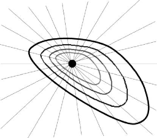
Figure 1. Generalised polar coordinates $(F,\theta)$: First coordinate lines are $\{F=\operatorname{const}\}$, second coordinate lines are rays from zero. The second coordinate is chosen such that on $\{F=1\}$ it corresponds to the $g$-arclength parameter.

If $E=\tfrac{1}{2}(x_{1}^{2}+x_{2}^{2})$ (so that $g=dx_{1}^{2}+dx_{2}^{2}$), generalised polar coordinates are the usual polar coordinates. In the general case, $\theta$ is still periodic and is defined up to addition of a constant to $\theta$ and the change of the sign, but the period is not necessary $2\pi$.

In the generalised polar coordinates, the Hessian metric $g=\tfrac{1}{2}{\rm d}^{2}(F^{2})={\rm d}F^{2}+F^{2}d\theta^{2}$ is flat. So we see that any two 2-dimensional Minkowski norms are locally Hessian-isometric, and are Hessian-isometric if and only if their indicatrices have the same length in the corresponding Hessian metrics.

Let us now consider $n\geq 3$. This case is almost completely open: in the literature we found one nonlinear example of Hessian isometry, which we will recall and generalise later, and one negative result, which is the following Theorem:

Theorem 1.1 ([13], for alternative proof see [39]).

Let $F$ be a Minkowski norm on $\mathbb{R}^{n}$, $n\geq 3$. Assume it is absolutely homogeneous, that is $F(\lambda y)=|\lambda|\cdot F(y)$ for every $\lambda\in\mathbb{R}$ and $y\in\mathbb{R}^{n}$.

Then, if the Hessian metric $g=\tfrac{1}{2}{\rm d}^{2}(F^{2})$ on $\mathbb{R}^{n}\backslash\{0\}$ has zero curvature, $F$ is Euclidean, that is, $F={\sqrt{\sum_{i,j}\alpha_{ij}x_{i}x_{j}}}$ for a positive definite symmetric matrix $(\alpha_{ij})\in\mathbb{R}^{n\times n}$. In this case, every Hessian isometry is linear.

The proofs in [13, 39] are different, but the assumption that $F$ is absolutely homogeneous is essential for both.

Let us now recall and slightly generalise the only known example of nonlinear Hessian isometry in dimension $n\geq 3$. We start with any Minkowski norm $F$ on the space $\mathbb{R}^{n}$ of column vectors, set $E=\tfrac{1}{2}F^{2}$ and consider the corresponding Legendre transformation:

$$\Phi:\mathbb{R}^{n}\setminus\{0\}\to\mathbb{R}^{n}\setminus\{0\}\ ,\ \ y=(x_{1},...,x_{n})^{T}\mapsto\left(\tfrac{\partial}{\partial x_{1}}E(y),...,\tfrac{\partial}{\partial x_{n}}E(y)\right)^{T}.$$ (1.1)

For the Euclidean Minkowski norm $F=\sqrt{x_{1}^{2}+...+x_{n}^{2}}$, the Legendre transformation $\Phi=\textrm{id}$.

Obviously the function $\hat{E}=\Phi_{*}(E)$ on $\mathbb{R}^{n}\backslash\{0\}$ is a positive smooth function satisfying the positive 2-homogeneity. As we explain below in Remark 1.2 (see also [8, §4.8]), the Hessian of $\hat{E}$ is given by the matrix inverse to that for $g$ and is therefore positive definite. Then, $\hat{F}=\sqrt{2\hat{E}}$ is a Minkowski norm.

In [40] it was proved that the Legendre transformation $\Phi$ in (1.1) is a Hessian isometry from $F$ to $\hat{F}$. Clearly, it is linear if and only if $F$ is Euclidean.

Remark 1.2.

R. Schneider’s observation that the Legendre transformation $\Phi$ in (1.1) is a Hessian isometry is important for our paper, so let us sketch a proof. Using $g_{ij}=\tfrac{\partial^{2}E}{\partial x_{i}\partial x_{j}}$ for the Hessian metric of $F$ and the explained above formula $E=\tfrac{1}{2}\sum_{i,j}g_{ij}x_{i}x_{j}$, the Legendre transformation $\Phi$ in (1.1) can be presented at $y=(x_{1},\cdots,x_{n})^{T}\in\mathbb{R}^{n}\backslash\{0\}$ as (see e.g. [8, Eq. (14.8.1)])

$$\Phi(y)=\left(\tfrac{\partial}{\partial x_{j}}\tfrac{1}{2}\sum_{i,k}g_{ik}x_{i}x_{k}\right)_{1\leq j\leq n}=\left(\sum_{i}g_{ij}x_{i}+\tfrac{1}{2}\sum_{i,k}\tfrac{\partial g_{ik}}{\partial x_{j}}x_{i}x_{k}\right)_{1\leq j\leq n}=\left(\sum_{i}g_{ij}x_{i}\right)_{1\leq j\leq n}.$$

Here we have used $\sum_{i}\tfrac{\partial g_{ik}}{\partial x_{j}}x_{i}x_{k}=x_{k}\left(\sum_{i}\tfrac{\partial g_{ik}}{\partial x_{j}}x_{i}\right)=0$ by the positive $2$-homogeneity of $E$. Then, its differential $d\Phi$ at $y$ has the Jacobi matrix

$$\left(d\Phi\right)_{1\leq i,j\leq n}=\left(g_{ij}+\sum_{k}\tfrac{\partial g_{ik}}{\partial x_{j}}x_{k}\right)_{1\leq i,j\leq n}=\left(g_{ij}\right)_{1\leq i,j\leq n}.$$

Since the Legendre transformation is an involution, $\Phi^{-1}$ is the Legendre transformation in (1.1) with $F=\hat{\hat{F}}$ and $\hat{F}$ exchanged, the Hessian metric $\hat{g}$ for $\hat{F}$ at $\Phi(x)$ is represented by the inverse matrix $(g^{ij})_{1\leq i,j\leq n}$ for $F$ at $x$ (see [8, Proposition 14.8.1] for more details). So the pullback $\Phi^{*}\hat{g}$ is given by the matrix

$$\left(\sum_{s,r}g^{sr}g_{si}g_{rj}\right)_{1\leq i,j\leq n}=\left(g_{ij}\right)_{1\leq i,j\leq n},$$

which is the matrix of the Hessian metric $g$ for $F$.

Let us now modify the above example. We start with the Euclidean Minkowski norm $F_{0}=\sqrt{x_{1}^{2}+\cdots+x_{n}^{2}}$, and slightly deform it on two conic open subsets $C(U_{1})$ and $C(U_{2})$ of $\mathbb{R}^{n}\backslash\{0\}$, where $U_{1}$ and $U_{2}$ are two open subsets of $S_{F_{0}}$ with disjoint closures. We obtain a new Minkowski norm $F_{1}$. Denote by $\Phi$ the Legendre transformation and by $\hat{F}_{1}$ the push-forward of $F_{1}$. See Fig. 2. The second new Minkowski norm $F_{2}$ is constructed as follows: it coincides with $\hat{F}_{1}$ on $C(U_{2})$ and with $F_{1}$ on $\mathbb{R}^{n}\backslash C(U_{2})$. It is still a smooth strictly convex Minkowski norm. Next, we consider the mapping $\tilde{\Phi}$ such that it is identity on $C(U_{1})$ and $\Phi$ on $\mathbb{R}^{n}\backslash C(U_{1})$. It is a Hessian isometry from $F_{1}$ to $F_{2}$. If $F_{1}$ is different from $F_{0}$ on both $C(U_{1})$ and $C(U_{2})$, $\tilde{\Phi}$ is neither a linear isometry nor a Legendre transform.

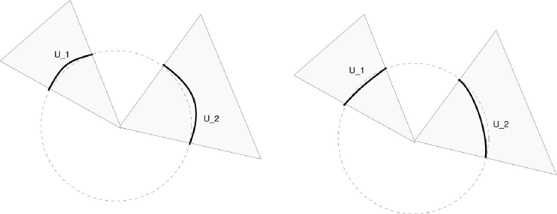
Figure 2. Construction of nonlinear and nonlegendre Hessian isometry: the functions $E_{1}=E$ is different from $x_{1}^{2}+...+x_{n}^{2}$ in cones over $U_{1}$ and $U_{2}$ (grey triangles). The function $\hat{E}$ (second picture) is the Legendre-transform of $E=E_{1}$. The function $E_{2}$ coincides with $E_{1}$ everywhere but in $C(U_{2})$ and in $C(U_{2})$ it coincides with $\hat{E}$

One can build this example such that $F_{1}$ and $F_{2}$ are preserved by the standard blockdiagonal action of $O(k)\times O(n-k)$ (of course in this case the conic open sets $C(U_{i})$ must be $O(k)\times O(n-k)$-invariant). One can impose additional symmetries on the construction so the resulting metric $F_{2}$ has, in addition to this linear $O(k)\times O(n-k)$-symmetry, a nonlinear Hessian self-isometry. One can further generalise this example by starting with $F_{0}$ which is not Euclidean but still has ‘Euclidean pieces’ and by deforming $F_{0}$ in more than two (even infinitely many) open subsets.

1.2. Results

We consider a Minkowski norm $F$ on $\mathbb{R}^{n}$ with $n\geq 3$ which has a linear $SO(k)\times SO(n-k)$-symmetry, and study connected isometry group (i.e., the identity component of the group of all isometries) of the Hessian metric of $F$. We prove:

Theorem 1.3.

Suppose $F$ is a Minkowski norm on $\mathbb{R}^{n}$ with $n\geq 3$, which is invariant with respect to the standard block diagonal action of the group $SO(k)\times SO(n-k)$ with $1\leq k\leq n-1$. Let $G_{0}$ be the connected isometry group for the Hessian metric $g=\tfrac{1}{2}{\rm d}^{2}F^{2}$ on $\mathbb{R}^{n}\backslash\{0\}$.

Then, every element $\Phi\in G_{0}$ is linear. Moreover, if $F$ is not Euclidean, then $G_{0}$ together with its action coincides with $SO(k)\times SO(n-k)$.

In Theorem 1.3, the standard block diagonal $SO(k)\times SO(n-k)$-action is the left multiplication on column vectors by all block diagonal matrices $\mathrm{diag}(A^{\prime},A^{\prime\prime})$ with $A^{\prime}\in SO(k)$ and $A^{\prime\prime}\in SO(n-k)$.

Theorem 1.3 is sharp in the following sense:

• By an $SO(k)\times SO(n-k)$-equivariant modification for the Legendre transformation we have discussed at the end of Section 1.1, we can construct some nonlinear Hessian isometry $\tilde{\Phi}$. So $G_{0}$ in Theorem 1.3 can not be changed to the full group $G$ of all Hessian isometries on $(\mathbb{R}^{n},F)$.

• If $F$ is Euclidean, i.e., $F=\sqrt{\sum_{i,j}\alpha_{ij}x_{i}x_{j}}$ for some positive definite symmetric matrix $(\alpha_{ij})$, its Hessian metric $g$ on $\mathbb{R}^{n}\backslash\{0\}$ is the restriction of a flat metric on $\mathbb{R}^{n}$. In this case the group of all Hessian isometries is $O(n)$ and the connected isometry group $G_{0}$ is $SO(n)$.

• Theorem 1.3 is not true locally. In Remark 2.5 we will show the existence of (smooth positively 1-homogeneous strongly convex $SO(2)$-invariant) functions $F$ defined on a conic open subset of $\mathbb{R}^{3}\backslash\{0\}$ such that it is not Euclidean but the corresponding Hessian metric is flat. See also discussion in Section 1.5.

• Theorem 1.3 and also other results of our paper trivially hold when $k=0$ or $k=n$, since in this case the Minkowski norm is automatically Euclidean. In the proofs we assume without loss of generality $1\leq k\leq n/2$.

Theorem 1.3 implies that for any two non-Euclidean Minkowski norms $F_{1}$ and $F_{2}$ which are invariant with respect to the standard blockdiagonal action of the group $SO(k)\times SO(n-k)$, with $n\geq 3$ and $1\leq k\leq n-1$, a Hessian isometry $\Phi$ from $F_{1}$ to $F_{2}$ must map orbits to orbits (i.e., $\Phi$ maps each $SO(k)\times SO(n-k)$-orbit to an $SO(k)\times SO(n-k)$-orbit).

Next, we consider two Minkowski norms $F_{1}$ and $F_{2}$ on $\mathbb{R}^{n}$ which are invariant for the standard block diagonal action of $SO(k)\times SO(n-k)$, and study local Hessian isometry which maps orbits to orbits. That means the local Hessian isometry $\Phi$ from $F_{1}$ to $F_{2}$ is defined between two $SO(k)\times SO(n-k)$-invariant conic open sets, $C(U_{1})$ and $C(U_{2})$, under the additional assumption that $\Phi$ maps each $SO(k)\times SO(n-k)$-orbit in $C(U_{1})$ to that in $C(U_{2})$.

Theorem 1.4.

Let $F_{1}$ be a Minkowski norm on $\mathbb{R}^{n}$ which is invariant for the standard block diagonal $SO(k)\times SO(n-k)$-action, with $n\geq 3$ and $1\leq k\leq n-1$. Assume $C(U_{1})$ is an $SO(k)\times SO(n-k)$-invariant connected conic open subset of $\mathbb{R}^{n}\backslash\{0\}$, such that every $y\in C(U_{1})$ satisfies

$$g_{1}(v^{\prime},v^{\prime\prime})\neq 0,\quad\mbox{for some }v^{\prime}\in V^{\prime}\mbox{ and }v^{\prime\prime}\in V^{\prime\prime}.$$ (1.2)

Here $g_{1}=g_{1}(\cdot,\cdot)$ is the Hessian metric of $F_{1}$, and $\mathbb{R}^{n}=V^{\prime}\oplus V^{\prime\prime}$ is an $SO(k)\times SO(n-k)$-invariant decomposition with $\dim V^{\prime}=k$ and $\dim V^{\prime\prime}=n-k$.

Then, for any $SO(k)\times SO(n-k)$-invariant Minkowski norm $F_{2}$, and any local Hessian isometry $\Phi$ from $F_{1}$ to $F_{2}$ which is defined on $C(U_{1})$ and maps orbits to orbits, $\Phi$ either coincides with the restriction of a linear isometry, or it coincides with the restriction of the composition of the $F_{1}$-Legendre transformation and a linear isometry.

Let us emphasize that near the points such that (1.2) holds the Minkowski norm $F$ is not Euclidean so the $F_{1}$-Legendre transformation is not linear. In particular, $\Phi$ can not be simultaneously linear and the composition of the the $F_{1}$-Legendre transformation and a linear isometry.

The condition (1.2) in Theorem 1.4 characterizes one class of generic points on $S_{F_{1}}$ where $S_{F_{1}}$ does not touch any $O(k)\times O(n-k)$-invariant ellipsoid with an order bigger than one. Of course, (1.2) is an open condition. But still the set of the points such that (1.2) is not fulfilled (for all $v^{\prime}$ and $v^{\prime\prime}$) may contain nonempty open subset. We discuss such open domains in the following Theorem:

Theorem 1.5.

Let $F_{1}$ be a Minkowski norm on $\mathbb{R}^{n}$ which is invariant for the standard block diagonal $SO(k)\times SO(n-k)$-action, with $n\geq 3$ and $1\leq k\leq n-1$. Assume $C(U_{1})$ is an $SO(k)\times SO(n-k)$-invariant connected conic open subset of $(\mathbb{R}^{n}\backslash\{0\},g_{1})$ such that at every $y\in C(U_{1})$

$$g_{1}(v^{\prime},v^{\prime\prime})=0,\quad\mbox{for all }v^{\prime}\in V^{\prime}\mbox{ and }v^{\prime\prime}\in V^{\prime\prime}.$$ (1.3)

Here $g_{1}=g_{1}(\cdot,\cdot)$ is the Hessian metric of $F_{1}$, and $\mathbb{R}^{n}=V^{\prime}\oplus V^{\prime\prime}$ is an $SO(k)\times SO(n-k)$-invariant decomposition with $\dim V^{\prime}=k$ and $\dim V^{\prime\prime}=n-k$.

Then the restriction of $F_{1}$ to $C(U_{1})$ is Euclidean. Moreover, for any $SO(k)\times SO(n-k)$-invariant Minkowski norm $F_{2}$, and any local Hessian isometry $\Phi$ from $F_{1}$ to $F_{2}$ which is defined on $C(U_{1})$ and maps orbits to orbits, we have that $\Phi$ coincides with the restriction of a linear isometry and that the restriction of $F_{2}$ to $C(U_{2})=\Phi(C(U_{1}))$ is Euclidean.

The example discussed in Remark 2.5 shows that the condition that $\Phi$ maps orbits to orbits is necessary for Theorem 1.5.

Theorem 1.4 and Theorem 1.5 provide the precise and explicit description for a local (or global) Hessian isometry $\Phi$ almost everywhere in its domain. We can find two $SO(k)\times SO(n-k)$-invariant conic open subsets $C({U}^{\prime})$ and $C({U}^{\prime\prime})$ in $\mathbb{R}^{n}\backslash\{0\}$, such that $C({U}^{\prime})\cup C({U}^{\prime\prime})$ is dense in the domain of $\Phi$, (1.2) is satisfied on $C({U}^{\prime})$, and (1.3) is satisfied on $C({U}^{\prime\prime})$. Then by these two theorems, when restricted to each connected component $C(U^{\prime}_{1})$ of $C(U^{\prime})$, $\Phi$ is a linear isometry or the composition of the Legendre transformation of $F_{1}$ which we denote by $\Psi$ and a linear isometry. Restricted to each connected component of $C(U^{\prime\prime})$, $\Phi$ is a linear isometry. This implies that every such $\Phi$ can be constructed along the lines discussed at the end of Section 1.1.

1.3. Applications in convex geometry: a special case of Laugwitz Conjecture.

It was conjectured by D. Laugwitz [29, page 70] that Theorem 1.1 remains true without the assumption of absolute homogeneity:

Conjecture 1.6 (Laugwitz Conjecture).

If the Hessian metric $g=\tfrac{1}{2}{\rm d}^{2}F^{2}$ for a Minkowski norm $F$ is flat on $\mathbb{R}^{n}\backslash\{0\}$ with $n\geq 3$, then $F$ is Euclidean.

For a discussion from the viewpoint of Finsler geometry see e.g. [8, Remark (b) on page 416]. Using Theorem 1.3, we prove the following special case of Laugwitz Conjecture.

Corollary 1.7.

Laugwitz conjecture is true for the class of Minkowski norms which are invariant with respect to the standard block diagonal $SO(n-1)$-action.

Indeed, if the Hessian metric of $F$ is flat on $\mathbb{R}^{n}\backslash\{0\}$, then the identity component $G_{0}$ of all Hessian isometries for $F$ has the dimension $\tfrac{n(n-1)}{2}$. As a Lie group, $G_{0}$ is isomorphic to $SO(n)$, but its action on $\mathbb{R}^{n}$ is linear iff $F$ is Euclidean. Since we have assumed here that $F$ is invariant with respect to the standard block diagonal action of $SO(n-1)=SO(1)\times SO(n-1)$ with $n\geq 3$, and obviously $G_{0}=SO(n)$ has a bigger dimension than $SO(n-1)$, the last statement in Theorem 1.3 for $k=1$ or $k=n-1$ guarantees that the $G_{0}$-action is linear in this case.

By similar argument, it follows from Theorem 1.3 that the Laugwitz conjecture is true for Minkowski norms which are invariant for the standard block diagonal $SO(k)\times SO(n-k)$-action with $2\leq k\leq n-2$. Notice that it has already been covered by Theorem 1.1, because the norms are absolutely homogeneous in this case.

1.4. Application in Finsler geometry: a special case of Landsberg Unicorn Conjecture

Historically Finsler geometry appeared as an attempt of generalising results and methods from Riemannian geometry to the optimal transport and calculus of variation, see e.g. [9, 11, 14, 24, 28, 38]. Generalisation of Riemannian results to the Finslerian setup is still one of the most popular research directions in Finsler geometry, and one of the main sources for interesting problems and methods.

The analogs of Riemannian objects in Finsler geometry are in many cases more complicated than Riemannian originals [43]. The connection (actually, there are three main natural candidates for the generalisation of the Levi-Civita connection) is generically not linear. It results in the nonlinearity for the Berwald parallel transport, which will be addressed later. The analogs of the Riemannian curvatures are also more complicated and in fact there exist two main different types of the curvature: the Riemannian type and the non-Riemannian type. For example, the flag curvature, which generalizes the sectional curvature in Riemannian geometry, is of the Riemannian type. On the other hand, the Landsberg curvature is of the non-Riemannian type, because it vanishes identically for Riemannian metrics and has no analogs in Riemannian geometry.

It is known that the Landsberg curvature vanishes identically for a relatively small class of Finsler metrics called Berwald metrics, which are characterized by the property that the Berwald parallel transport is linear, see e.g. [16, Proposition 4.3.2] or [8, §10]. Berwald metrics are completely understood, see e.g. [16, Theorem 4.3.4], [35, §§8,9] or [46].

A non-Berwald Finsler metric with vanishing Landsberg curvature is called a unicorn metric. Many experts believe that smooth unicorn metrics do not exist. This statement is called the Landsberg Unicorn Conjecture.

Conjecture 1.8 (Landsberg Unicorn Conjecture).

A Finsler metric with vanishing Landsberg curvature must be Berwald.

The origin of this conjecture can be traced back to [10] (or even to [28]). It is definitely one of the most popular open problems in Finsler geometry and was explicitly asked in e.g. [1, 6, 7, 21, 32, 44]. Its proof was reported a few times in preprints and even published in reasonable journals, but later crucial mistakes were found, see e.g. [33].

The definition of the Landsberg curvature and the properties of Finsler metrics with vanishing Landsberg curvature can be found elsewhere, e.g. in [16, §2.1 and §4.4]. For our paper, we only need the following known statement:

Fact 1.9 (e.g. Proposition 4.4.1 of [16] or [27]).

If Landsberg curvature vanishes, then the Berwald parallel transport is isometric with respect to the Hessian metric (corresponding to $E=\tfrac{1}{2}F^{2}$ in each tangent space).

Recall that the Berwald parallel transport is a Finslerian analog of the parallel transport in Riemannian geometry. For every smooth curve $c:[0,1]\to M$ on $(M,F)$, the Berwald parallel transport along $c$ provides a smooth family of diffeomorphisms $\Phi_{s}:T_{c(0)}M\backslash\{0\}\to T_{c(s)}M\backslash\{0\}$. Similarly to the Riemannian case, the mapping is defined via certain system of ODEs along the curve $c$. Differently from the Riemannian case, these ODEs are not linear, so for a generic Finsler metric the Berwald parallel transport is not linear as well. In fact, as recalled above, it is linear if and only if the metric is Berwald.

In Section 4 we explain that Theorems 1.3, 1.4 and 1.5 easily imply the following important special case of Conjecture 1.8.

Corollary 1.10.

Let $(M,F)$ be a Finsler manifold of dimension $n\geq 3$. Assume that for every point $p\in M$, there exist linear coordinates in $T_{p}M$ such that the restriction $F_{|T_{p}M}$ is invariant with respect to the standard block diagonal action of the group $SO(k)\times SO(n-k)$ with $1\leq k\leq n-1$.

Then, if the Landsberg curvature vanishes, $F$ is Berwald.

Many special cases of Corollary 1.10 appeared in the literature before. Let us give some examples with the dimension $n\geq 3$: [31] (see also [26]) proved that every Randers metric such that its Landsberg curvature is zero is Berwald. [45] proved that every $(\alpha,\beta)$ metric with zero Landsberg curvature is Berwald. [49] proved that every general $(\alpha,\beta)$ metric with zero Landsberg curvature is Berwald. All these results follow from Corollary 1.10 with $k=1$, since for every $p\in M$ the restriction of a Randers, $(\alpha,\beta)$ or general $(\alpha,\beta)$ metric to $T_{p}M$ is invariant with respect to a block diagonal action of $SO(n-1)$ [19]. Indeed, general $(\alpha,\beta)$ is defined as follows: one takes a Riemannian metric $\alpha=(a_{ij})$, a $1$-form $\beta=(\beta_{i})$, a function $\varphi$ of two varables, and defines $F$ by the formula

$$F(p,y)=\varphi\left(|\beta|_{\alpha},\frac{\beta(y)}{\sqrt{\alpha(y,y)}}\right)\sqrt{\alpha(y,y)},$$ (1.4)

where $|\beta|_{\alpha}=\sqrt{\alpha^{ij}\beta_{i}\beta_{j}}$ is the point-wise norm of $\beta$ in $\alpha$ and $\alpha(y,y)=\alpha_{ij}y^{i}y^{j}=\left(|y|_{\alpha}\right)^{2}$. The function $\varphi$ is chosen such that (1.4) is a Finsler metric. For certain $\varphi$, additional restrictions on $|\beta|_{\alpha}$ must be assumed to insure the result is a Finsler metric. chosen such that (1.4) is a Finsler metric. For certain $\varphi$, additional restrictions on $|\beta|_{\alpha}$ must be assumed to insure the result is a Finsler metric.

$(\alpha,\beta)$ metrics are general $(\alpha,\beta)$ metrics such that the function $\varphi$ does not depend on $|\beta|_{\alpha}$ (so it is a function of one variable). Randers metrics are $(\alpha,\beta)$ metrics for the function $\varphi(t)=1+\tfrac{1}{t}$. In the last case the restriction insuring that this $\varphi$ determines a Finsler metric is $|\beta|_{\alpha}<1$.

Note that the proofs from [31, 45, 49] essentially use that the function $\varphi(t,s)$ is the same at all points of the manifold, so the dependence of Randers, $(\alpha,\beta)$ and general $(\alpha,\beta)$ metrics on the position $p\in M$ essentially goes through the dependence of $\alpha$ and $\beta$ on $p$ only. In our proof we need only that in each tangent space $F$ has a linear $SO(n-1)$-symmetry. In other words, the function $\varphi$ may arbitrary depend on the point $p$ of the manifold.

Another example of such type is [20, 47]: there, the so-called $(\alpha_{1},\alpha_{2})$ metrics are considered, their definition which we do not recall here is similar to that of $(\alpha,\beta)$ metrics. In this case, the restriction of the metric to each tangent space is invariant with respect to the $SO(k)\times SO(n-k)$-action. The analog of the function $\varphi$ is the same at all points of the manifold so the dependence of the metric on position goes through $\alpha_{1}$ and $\alpha_{2}$ only. By our result, the function $\varphi$ may arbitrarily depend on the position.

A slightly different result which also follows from Corollary 1.10 is in [36], where nonexistence of non-Berwaldian Finsler manifolds with vanishing Landsberg curvature was shown in the class of spherically symmetric metrics. By definition, Finlser metric on $\mathbb{R}^{n}\setminus\{0\}$ is spherically symmetric, if it is invariant with respect to the standard action of $SO(n)$. This condition implies that the restriction of $F$ to every tangent space has $SO(n-1)$-symmetry and Corollary 1.10 is applicable.

Alternative geometric approach that was successfully used for the proof of Landsberg Unicorn Conjecture for certain generalisations of $(\alpha,\beta)$ metrics is based on semi-C-reducibility [18, 22, 34]. The results of these papers related to the Landsberg Unicorn Conjecture also easily follow from our Corollary 1.10. Notice that generic $(\alpha_{1},\alpha_{2})$ metrics do not satisfy the semi-C-reducibility.

1.5. Smoothness assumption is necessary.

G. Asanov constructed some singular norms $F$ on $\mathbb{R}^{3}$ with the standard $SO(2)$-symmetry [2, 3] His examples can be generalised to any dimension $n\geq 3$ and give singular norms on $\mathbb{R}^{n}$ with linear $SO(n-1)$-symmetry, see e.g. [49]. They lead to the construction of first singular unicorn metrics [4, 5] and were actively discussed in the literature (e.g. [17]).

The Minkowski norms in all these examples are not smooth at the line which is fixed by the $SO(n-1)$-action, but they are smooth and even real analytic elsewhere. Their isometry group is $O(n-1)$ but locally the algebra of Killing vector fields is isomorphic to $so(n)$ and has the dimension $\tfrac{(n-1)n}{2}$.

Within this paper we assume that all objects we consider are sufficiently smooth. Asanov’s examples and their generalisations show that this smoothness assumption is necessary. It also shows (complimentary to Remark 2.5) that Theorem 1.3 is not a local statement.

2. Hessian isometry on a Minkowski space with $SO(k)\times SO(n-k)$-symmetry

2.1. Setup.

Within the whole section we work in a Minkowski space $(\mathbb{R}^{n},F)$ with $n\geq 3$. We denote $S_{F}=\{y\in\mathbb{R}^{n}\mid F(y)=1\}$ the indicatrix of $F$, and $g$ the Hessian metric $\tfrac{1}{2}{\rm d}^{2}F^{2}$ of $F$ on $\mathbb{R}^{n}\backslash\{0\}$ or its restriction to $S_{F}$ (and other submanifolds). We assume that $F$ is invariant with respect to the standard block diagonal action of $SO(k)\times SO(n-k)$, with $1\leq k\leq n/2$.

We start with the following simple observation:

Lemma 2.1.

Suppose $F$ is a Minkowski norm on $\mathbb{R}^{n}$ which is invariant with respect to the standard block diagonal action of $SO(k)\times SO(n-k)$ with $n\geq 3$ and $1\leq k\leq n/2$. Then $F$ is invariant with respect to the standard block diagonal action of $O(n-1)$ or $O(k)\times O(n-k)$ when $k=1$ or $k>1$ respectively.

Note that $SO(1)=\{e\}$ so the action of $O(n-1)=SO(1)\times O(n-1)$ is just that by the orthogonal matrices of the form $\mathrm{diag}(1,A)$ with $A\in O(n-1)$.

Proof. Clearly, when $k\neq 1$, the orbits of the action of $SO(k)\times\{e\}$ coincide with that of $O(k)\times\{e\}$, so the function $F$, which is invariant with respect to the action of $SO(k)\times\{e\}$, is also invariant with respect to the action of $O(k)\times\{e\}$. Similarly, by $k\leq n/2\leq n-2$, $F$ is invariant with respect to the action of $\{e\}\times O(n-k)$.   

2.2. Proof of Theorem 1.3 for $k=1$.

We consider the indicatrix $S_{F}$ with the restriction of the Hessian metric $g$. Let $G_{0}$ be the connected isometry group for $(\mathbb{R}^{n}\backslash\{0\},g)$, then it is also the connected isometry group for $(S_{F},g)$. We assume that $F$ is invariant with respect to the standard block diagonal action of $SO(n-1)$. It implies that $G_{0}$ naturally contains the group $SO(n-1)$ as a subgroup.

If $G_{0}$ coincides with $SO(n-1)$, there is nothing to prove. The next Lemma shows that if $G_{0}$ does not coincide with $SO(n-1)$ then $(S_{F},g)$ is isometric to the standard unit sphere.

Lemma 2.2.

In the notation above, assume $G_{0}$ does not coincide with $SO(n-1)$. Then $(\mathbb{R}^{n}\backslash\{0\},g)$ is flat, and $(S_{F},g)$ has constant sectional curvature 1.

Proof. Let us assume that $G_{0}$ does not coincide with $SO(n-1)$, i.e., $\dim G_{0}\geq\tfrac{(n-1)(n-2)}{2}+1$.

We first prove that $(S_{F},g)$ is a homogeneous Riemannian sphere. Here we apply a proof of this claim for all $n\geq 3$, which is similar to that of [48, Theorem 1], see also [25, §4]. Notice that when $n\neq 5$, [48, Theorem 1] provides an alternative approach. Indeed, we can also see that $(S_{F},g)$ has constant sectional curvature, by [37, Theorem 10] and [25, Theorem 5] when $n\neq 5$ and $n=5$ respectively, though it would not be needed in later argument.

Consider the “pole” $y_{0}=(a_{0},0,...,0)\in S_{F}$. It is a fixed point for the $SO(n-1)$-action. Consider its $G_{0}$-orbit

$$G_{0}\cdot y_{0}=\{\Phi(y_{0})\mid\Phi\in G_{0}\}.$$

Let $H\subset G_{0}$ be the stabilizer of $y_{0}$. It is known that the stabilizer of a point with respect to an isometric action on an $(n-1)$-dimensional manifold is at most $\tfrac{(n-1)(n-2)}{2}$-dimensional, so we have $\dim G_{0}>\tfrac{(n-1)(n-2)}{2}\geq\dim H$, i.e., there exists $y\in G_{0}\cdot y_{0}$ with $y\neq y_{0}$. The orbit $G_{0}\cdot y_{0}$ is connected, so we can find a curve $\gamma\subset G_{0}\cdot y_{0}$ connecting $y$ and $y_{0}$. Then $G_{0}\cdot y_{0}\supset SO(n-1)\cdot\gamma$ contains a $SO(n-1)$-invariant neighbourhood $U_{0}$ of $y_{0}$ in $S_{F}$. By its homogeneity, $G_{0}\cdot y_{0}$ is an open subset of $S_{F}$. On the other hand, it is closed because $G_{0}$ is a compact Lie group. So we must have $G_{0}\cdot y_{0}=S_{F}$, i.e., $(S_{F},g)$ is a homogeneous sphere.

Next, we prove that the Hessian metric $g$ on $\mathbb{R}^{n}\backslash\{0\}$ is flat, and its restriction to $S_{F}$ has constant curvature 1.

The Cartan tensor at $y=(x_{1},\cdots,x_{n})\in\mathbb{R}^{n}\backslash\{0\}$ is defined as

$$C(u,v,w)=\tfrac{1}{4}\tfrac{\partial^{3}}{\partial s_{1}\partial s_{2}\partial s_{3}}_{|s_{1}=s_{2}=s_{3}=0}F(y+s_{1}u+s_{2}v+s_{3}w)^{2}.$$

for any $u,v,w\in\mathbb{R}^{n}=T_{y}\mathbb{R}^{n}$ (so its $(ijk)$-component is $C_{ijk}=\tfrac{1}{4}\tfrac{\partial^{3}(F^{2})}{\partial x_{i}\partial x_{j}\partial x_{k}}$).

Now we show the Cartan tensor vanishes at $y_{0}=(a_{0},0,\cdots,0)\in S_{F}$.

Clearly, it is multiple linear and totally symmetric. By the positive $1$-homogeneity of $F$, at every point $y\in\mathbb{R}^{n}\setminus\{0\}$ and for every vectors $u,v\in\mathbb{R}^{n}$, we have $C(y,u,v)=0$ at $y$. So we only need to show, for each vector $v$ with zero $x_{1}$-coordinate (i.e., $v\in T_{y_{0}}S_{F}$), we have $C(v,v,v)=0$ at $y_{0}$. Cartan’s trick can be applied to avoid direct calculation. The group $SO(n-1)$ acts transitively on the unit $g$-sphere in $T_{y_{0}}S_{F}$. So there exists $A\in SO(n-1)$ with $Av=-v$. That means, the linear isometry induced by $A$ fixes $y_{0}$ and has a tangent map at $y_{0}$ mapping $v$ to $-v$. It preserves the Cartan tensor as well, so we have

$$C(v,v,v)=C(-v,-v,-v)=-C(v,v,v)$$

at $y_{0}$, which implies $C=0$ there.

Now we use the following well-known fact in Hessian geometry:

Fact 2.3 (e.g. Proposition 3.2 of [41]).

Consider the Hessian metric generated by a (not necessary 2-homogeneous) function $E$, $g={\rm d}^{2}E$. Then, its curvature tensor $R_{ijk\ell}$ is given by

$$R_{ijk\ell}=\tfrac{1}{4}\sum_{s,r}\left(\frac{\partial^{3}E}{\partial x_{j}\partial x_{\ell}\partial x_{s}}g^{sr}\frac{\partial^{3}E}{\partial x_{k}\partial x_{i}\partial x_{r}}-\frac{\partial^{3}E}{\partial x_{i}\partial x_{\ell}\partial x_{s}}g^{sr}\frac{\partial^{3}E}{\partial x_{k}\partial x_{j}\partial x_{r}}\right),$$ (2.5)

where $g^{rs}$ denote the components of the matrix inverse to $(g_{rs})$.

If $E=\tfrac{1}{2}F^{2}$ for a Minkowski norm $F$, the curvature formula (2.5) is reduced to

$$R_{ijk\ell}=\sum_{s,r}\left(C_{i\ell s}g^{sr}C_{jkr}-C_{iks}g^{sr}C_{j\ell r}\right).$$ (2.6)

As we explained above, at $y_{0}$, every $C_{ijk}$ vanishes, so we have $R_{ijk\ell}=0$, $\forall i,j,k,\ell$. In particular, the sectional curvature of $(\mathbb{R}^{n}\backslash\{0\},g)$ vanishes at $y_{0}$.

As we recalled in Section 1.1, the Hessian metric $g=({\rm d}F)^{2}+F^{2}g_{|S_{F}}$ on $\mathbb{R}^{n}\backslash\{0\}$ is the cone metric over its restriction to $S_{F}$. Then by Gauss-Codazzi equation, the sectional curvature of $(S_{F},g)$ equals to $1$ at $y_{0}$. Since $(S_{F},g)$ is homogeneous by assumptions, $(S_{F},g_{S_{F}})$ has constant sectional curvature 1 at every point, i.e., it is isometric to the standard unit sphere. Then, the metric $g$ is flat as we claimed.   

The next Lemma finishes the proof of Theorem 1.3 for $k=1$.

Lemma 2.4.

Let $F$ be a Minkowski norm on $\mathbb{R}^{n}$ with $n\geq 3$, which is invariant with respect to the standard block diagonal action of $O(n-1)$. Assume the curvature of the Hessian metric $g=\tfrac{1}{2}{\rm d}^{2}(F^{2})$ on $\mathbb{R}^{n}\backslash\{0\}$ identically vanishes. Then $F$ is Euclidean.

Proof. We first prove Lemma 2.4 when $n=3$.

We consider the spherical coordinates $(r,\theta,\phi)\in\mathbb{R}_{>0}\times(0,\pi)\times(\mathbb{R}/(2\mathbb{Z}\pi))$ on $\mathbb{R}^{3}$ determined by

$$x_{1}=r\cos\theta,\ \ x_{2}=r\sin\theta\cos\phi,\ \ x_{3}=r\sin\theta\sin\phi.$$

The $SO(2)$-action is the left multiplication on column vectors by matrices of the form

$$\begin{pmatrix}1&0&0\\ 0&\cos s&\sin s\\ 0&-\sin s&\cos s\end{pmatrix},$$

i.e., it fixes the $r$- and $\theta$-coordinates and shifts the $\phi$-coordinate. By its $SO(2)$-invariancy and homogeneity, the function $E=\tfrac{1}{2}F^{2}$ can be presented as

$$E=r^{2}f(\theta).$$ (2.7)

By the symmetry $(x_{1},x_{2},x_{3})\mapsto(x_{1},-x_{2},-x_{3})$ for $E$, the function $f(\theta)$ on $(0,\pi)$ can be extended to and will be viewed as an even positive smooth function on $\mathbb{R}$ with the period $2\pi$, i.e., the restriction of $E$ to the circle $\{(x_{1},x_{2},0)\mid x_{1}=\cos s,x_{2}=\sin s,\forall s\in\mathbb{R}\}$.

Let us now calculate the Hessian metric $g$ and the Cartan tensor $C$ of $F$ in the spherical coordinates. We use subscripts and superscripts $r$, $\theta$ and $\phi$, for example, $g_{r\theta}=g(\tfrac{\partial}{\partial r},\tfrac{\partial}{\partial\theta})$, and $C_{\theta\theta\phi}=C(\tfrac{\partial}{\partial\theta},\tfrac{\partial}{\partial\theta},\tfrac{\partial}{\partial\phi})$.

By its definition, $g$ is the second covariant derivative of $E$ with respect to the Levi-Civita connection of the standard flat metric on $\mathbb{R}^{3}$, so we have

$$g(X,Y)=X(Y(E))-(\tilde{\nabla}_{X}Y)(E),$$ (2.8)

for any smooth tangent vector fields $X$ and $Y$ on $\mathbb{R}^{3}\backslash\{0\}$, where $\tilde{\nabla}$ is the Levi-Civita connection for the standard flat metric

$$\tilde{g}:={\rm d}x_{1}^{2}+{\rm d}x_{2}^{2}+{\rm d}x_{3}^{2}={\rm d}r^{2}+r^{2}{\rm d}\theta^{2}+r^{2}\sin^{2}\theta{\rm d}\phi^{2}.$$

Direct calculation gives

$$\begin{array}[]{ll}\tilde{\nabla}_{\tfrac{\partial}{\partial r}}{\tfrac{\partial}{\partial r}}=0,&\tilde{\nabla}_{\tfrac{\partial}{\partial\theta}}{\tfrac{\partial}{\partial r}}=\tilde{\nabla}_{\tfrac{\partial}{\partial r}}{\tfrac{\partial}{\partial\theta}}=\tfrac{1}{r}\tfrac{\partial}{\partial\theta},\\ \tilde{\nabla}_{\tfrac{\partial}{\partial\phi}}{\tfrac{\partial}{\partial r}}=\tilde{\nabla}_{\tfrac{\partial}{\partial r}}{\tfrac{\partial}{\partial\phi}}=\tfrac{1}{r}\tfrac{\partial}{\partial\phi},&\tilde{\nabla}_{\tfrac{\partial}{\partial\theta}}{\tfrac{\partial}{\partial\theta}}=-r\tfrac{\partial}{\partial\phi},\\ \tilde{\nabla}_{\tfrac{\partial}{\partial\theta}}{\tfrac{\partial}{\partial\phi}}=\tilde{\nabla}_{\tfrac{\partial}{\partial\phi}}{\tfrac{\partial}{\partial\theta}}=\tfrac{\cos\theta}{\sin\theta}\tfrac{\partial}{\partial\phi},&\tilde{\nabla}_{\tfrac{\partial}{\partial\phi}}{\tfrac{\partial}{\partial\phi}}=-r\sin^{2}\theta\tfrac{\partial}{\partial r}-\sin\theta\cos\theta\tfrac{\partial}{\partial\theta}.\end{array}$$ (2.9)

Combining (2.7) and (2.8), we obtain all components $g_{ab}$, $a,b\in\{r,\theta,\phi\}$, for $g={\rm d}^{2}E$. With the specified order $(r,\theta,\phi)$, they can be presented as the following matrix,

$$\left[\begin{array}[]{ccc}2f(\theta)&r{\frac{\rm d}{{\rm d}\theta}}f(\theta)&0\\ \vskip 6.0pt plus 2.0pt minus 2.0pt\cr r{\frac{\rm d}{{\rm d}\theta}}f(\theta)&2r^{2}f(\theta)+r^{2}\frac{{\rm d}^{2}}{{\rm d}\theta^{2}}f(\theta)&0\\ \vskip 6.0pt plus 2.0pt minus 2.0pt\cr 0&0&2r^{2}\sin^{2}\theta f(\theta)+r^{2}\sin\theta\cos\theta\frac{\rm d}{{\rm d}\theta}f(\theta)\end{array}\right].$$ (2.10)

For further use, let us observe that the matrix (2.10) is block diagonal, so its inverse matrix is block diagonal as well, i.e., $g^{r\phi}=g^{\theta\phi}=0$ and $g^{\theta\theta}>0$.

To calculate the Cartan tensor $C_{abc}$ with $a,b,c\in\{r,\theta,\phi\}$, we can proceed analogically:

$$C(X,Y,Z)=\tfrac{1}{2}\left(Z(g(X,Y))-g(\tilde{\nabla}_{Z}X,Y)-g(X,\tilde{\nabla}_{Z}Y)\right).$$ (2.11)

Using (2.9) and (2.10), we see that the only possibly nonzero components of the Cartan tensor are

$$\begin{array}[]{rcl}C_{\theta\theta\theta}&=&2r^{2}\tfrac{{\rm d}}{{\rm d}\theta}f(\theta)+\tfrac{1}{2}r^{2}\tfrac{{\rm d}^{3}}{{\rm d}\theta^{3}}f(\theta),\\ C_{\theta\phi\phi}&=&-\tfrac{1}{2}r^{2}\cos 2\theta\tfrac{{\rm d}}{{\rm d}\theta}f(\theta)+\tfrac{1}{4}r^{2}\sin 2\theta\tfrac{{\rm d}^{2}}{{\rm d}\theta^{2}}f(\theta)\end{array}$$ (2.12)

(of course $C_{\theta\phi\phi}=C_{\phi\theta\phi}=C_{\phi\phi\theta}$ because $C$ is symmetric). Note that it is clear in advance that every component of the form $C_{r\cdot\cdot}=C(\tfrac{\partial}{\partial r},\cdot,\cdot)$ is zero, since $\tfrac{\partial}{\partial r}$ is the Euler vector field annihilating $C$. It is also clear by Cartan’s trick that the component $C_{\theta\theta\phi}$ is zero since the mapping given by $\phi\mapsto-\phi+\textrm{const}$ is in fact a linear isometry which from one side changes the sign for $C_{\theta\theta\phi}$ and from the other side preserves it.

In the case $n=3$, the only curvature component we need to consider is

$$R_{\theta\phi\phi\theta}=g(R(\tfrac{\partial}{\partial\theta},\tfrac{\partial}{\partial\phi})\tfrac{\partial}{\partial\phi},\tfrac{\partial}{\partial\theta})=\sum_{a,b\in\{r,\theta,\phi\}}(C_{\theta\theta a}g^{ab}C_{\phi\phi b}-C_{\theta\phi a}g^{ab}C_{\phi\theta b}).$$ (2.13)

Plugging (2.10) and (2.12) into (2.13) and using the vanishing of $g^{\theta\phi}$, $C_{r\cdot\cdot}$ and $C_{\theta\theta\phi}$, we get

$$R_{\theta\phi\phi\theta}=C_{\theta\theta\theta}g^{\theta\theta}C_{\theta\phi\phi}-C_{\theta\phi\phi}g^{\phi\phi}C_{\theta\phi\phi}.$$

So the vanishing of the Riemann curvature implies

$$C_{\theta\theta\theta}g^{\theta\theta}C_{\theta\phi\phi}-C_{\theta\phi\phi}g^{\phi\phi}C_{\theta\phi\phi}=0.$$ (2.14)

Note that the $\theta$-derivative of $C_{\theta\phi\phi}$ is $\tfrac{1}{2}\sin 2\theta\ C_{\theta\theta\theta}$. Indeed,

$$\tfrac{{\rm d}}{{\rm d}\theta}(\tfrac{C_{\theta\phi\phi}}{r^{2}}) = \tfrac{{\rm d}}{{\rm d}\theta}\left(-\tfrac{1}{2}\cos 2\theta\tfrac{{\rm d}}{{\rm d}\theta}f(\theta)+\tfrac{1}{4}\sin 2\theta\tfrac{{\rm d}^{2}}{{\rm d}\theta^{2}}f(\theta)\right)$$

$$= \tfrac{1}{2}\sin 2\theta\left(2\tfrac{{\rm d}}{{\rm d}\theta}f(\theta)+\tfrac{1}{2}\tfrac{{\rm d}^{3}}{{\rm d}\theta^{3}}f(\theta)\right)=\tfrac{1}{2}\sin 2\theta\cdot\tfrac{C_{\theta\theta\theta}}{r^{2}}.$$

Thus, $h(\theta)=\left(\tfrac{C_{\theta\phi\phi}}{r^{2}}\right)^{2}$ is the solution of the following ODE:

$$\tfrac{{\rm d}}{{\rm d}\theta}h(\theta)=\tfrac{g^{\phi\phi}\sin 2\theta}{g^{\theta\theta}}\cdot h(\theta)=\tfrac{\cos\theta\left(4f(\theta)^{2}+2f(\theta)\tfrac{{\rm d}^{2}}{{\rm d}t^{2}}f(\theta)-(\tfrac{{\rm d}}{{\rm d}t}f(\theta))^{2}\right)}{f(\theta)\left(2\sin\theta f(\theta)+\cos\theta\tfrac{{\rm d}}{{\rm d}t}f(\theta)\right)}\cdot h(\theta)$$ (2.15)

on $(0,\pi)$.

From (2.10) we see that $g_{\phi\phi}$ at the points of $S_{F}$, i.e., when $r^{2}=\tfrac{1}{2f(\theta)}$, is given by

$$\sin^{2}\theta+\tfrac{\sin\theta\cos\theta}{2f(\theta)}\tfrac{{\rm d}}{{\rm d}\theta}f(\theta).$$

In particular, we have $g_{\phi\phi}=1$ at $x\in S_{F}$ with $\theta$-coordinate equal to $\pi/2$. So the $g$-arc length of the curve $\{\theta=\pi/2\}$ on $S_{F}$ is $2\pi$. When we identify $(S_{F},g)$ with a standard $S^{2}(1)$, the $SO(2)$-action which shifts the $\phi$-coordinates on $S_{F}$ coincides with a standard linear $SO(2)$-action on $S^{2}(1)$ which orbits are the latitude lines. The curve $\theta=\pi/2$ on $S_{F}$ corresponds to the equator which has the maximal length among all latitude lines. So we have

$$\tfrac{{\rm d}}{{\rm d}\theta}\left(g_{\phi\phi}{}_{|r=(2f(\theta))^{-1/2}}\right)_{|\theta=\pi/2} = \tfrac{{\rm d}}{{\rm d}\theta}\left(\sin^{2}+\tfrac{\sin\theta\cos\theta}{2f(\theta)}\tfrac{{\rm d}}{{\rm d}\theta}f(\theta)\right)_{|\theta=\pi/2}$$

$$= -\tfrac{1}{2f(\pi/2)}\tfrac{{\rm d}}{{\rm d}\theta}f(\theta)_{|\theta=\pi/2}=0,$$

i.e., $\tfrac{{\rm d}}{{\rm d}\theta}f(\theta)_{|\theta=\pi/2}=0$. Plugging it into the formula of $C_{\theta\phi\phi}$ in (2.12), we see $C_{\theta\phi\phi}=0$ when $\theta=\pi/2$ and then $h(\pi/2)=0$. Thus, $h(\theta)$ satisfies the ODE (2.15) with the initial condition $h(\pi/2)=0$ so it is identically zero. Hence the Cartan tensor of $F$ vanishes identically which implies that the third partial derivatives of $F^{2}$ with respect to linear coordinates vanish so $F$ is Euclidean. Lemma 2.4 is proved for $n=3$.

Remark 2.5.

The equality (2.14) follows from (and is fact is equivalent to)

$$C_{\theta\theta\theta}g^{\theta\theta}-C_{\theta\phi\phi}g^{\phi\phi}=0$$ (2.16)

everywhere on $\mathbb{R}^{3}\backslash\{0\}$. This is a 3rd order ODE for $f(\theta)$, and has a 3-parameter family of local solutions. Among these local solutions, $c_{1}+c_{2}\cos 2\theta$ with appropriate constants $c_{1}$ and $c_{2}$ corresponds to the Euclidean norms. So we may generically perturb it among local solutions of (2.16), and use the resulting $f(\theta)$ to construct a flat Hessian metric $g={\rm d}^{2}E$ for $E=r^{2}f(\theta)$ in some conic open subset of $\mathbb{R}^{3}\backslash\{0\}$. Local Hessian isometries can be constructed between $g$ and the Hessian metric for an Euclidean norm. These local Hessian isometries are not linear.

Let us now prove Lemma 2.4 when $n>3$. Let $y_{0}\neq 0$ be any point fixed by the action of $O(n-1)$, and $V_{0}$ any 3-dimensional vector subspace containing $y_{0}$. We can find an involution in $O(n-1)$, such that $V_{0}$ is its fixed point set. Indeed, we can find suitable orthonormal coordinates $(x_{1},\cdots,x_{n})$ on $\mathbb{R}^{n}$, such that $V_{0}$ consists of all vectors $(x_{1},x_{2},x_{3},0,\cdots,0)$ and $y_{0}$ is presented by $(a_{0},0,\cdots,0)$. Then $V_{0}$ is the fixed point set of the mapping $(x_{1},\cdots,x_{n})\mapsto(x_{1},x_{2},x_{3},-x_{4},\cdots,-x_{n})$ in $O(n-1)$.

The restriction $F_{0}=F_{|V_{0}}$ is invariant with respect to the standard block diagonal action of $O(2)=SO(1)\times O(2)$. Its Hessian metric $g_{0}=\tfrac{1}{2}{\rm d}^{2}F_{0}^{2}=g_{|V_{0}\backslash\{0\}}$ is flat because it is the restriction of the ambient metric $g$ which is flat to a automatically totally geodesic fixed points set. Then, $F_{0}$ is Euclidean. By the $O(n-1)$-invariancy of $F$, we see that $F$ is Euclidean as well.   

2.3. Proof of Theorem 1.3 for $2\leq k\leq n/2$.

Assume now the Minkowski norm $F$ on $\mathbb{R}^{n}$ is invariant with respect to the standard block diagonal action on $O(k)\times O(n-k)$ with $2\leq k\leq n/2$. We denote by $G_{0}$ the connected isometry group for $(\mathbb{R}^{n}\backslash\{0\},g)$ and for $(S_{F},g_{|S_{F}})$.

We first consider the case when $(S_{F},g_{|S_{F}})$ is a homogeneous Riemannian sphere. As in the previous section, let us apply Cartan’s trick to prove that the Cartan tensor vanishes at the point $y_{0}=(a_{0},0,...,0)\in S_{F}$. Let $v\in\mathbb{R}^{n}$ be any vector contained in the tangent space $T_{y_{0}}S_{F}$, then its $x_{1}$-coordinate vanishes. The linear isometry $(x_{1},...,x_{n})\mapsto(x_{1},-x_{2},-x_{3}....,-x_{n})$ in $O(k)\times O(n-k)$ fixes $y_{0}$ and its tangent map at $y_{0}$ sends $v\in T_{y_{0}}S_{F}$ to $-v$. It preserves the Cartan tensor, so we have

$$C(v,v,v)=C(-v,-v,-v)=-C(v,v,v)$$

at $y_{0}$ for each $v\in T_{y_{0}}S_{F}$, which implies $C=0$ there.

Using (2.6) and the same argument as for Lemma 2.2, we see $(S_{F},g_{|S_{F}})$ has constant curvature 1 and $(\mathbb{R}^{n}\backslash\{0\},g)$ is flat. By $2\leq k\leq n/2$, we have $n\geq 4$, and the absolute 1-homogeneity for the $SO(k)\times SO(n-k)$-invariant Minkowski norm $F$. By Theorem 1.1, we obtain that $F$ is an Euclidean norm, which ends the proof of Theorem 1.3 when $(S_{F},g_{|S_{F}})$ is a homogeneous Riemannian sphere.

Next, we consider the case when $(S_{F},g_{|S_{F}})$ is not a homogeneous Riemannian sphere. Since the $SO(k)\times SO(n-k)$-action on $S_{F}$ has cohomogeneity one, $G_{0}$ must preserve each $SO(k)\times SO(n-k)$-orbit. Then the $G_{0}$-action maps normal geodesics on $(S_{F},g_{|S_{F}})$ (i.e., geodesics on $(S_{F},g_{|S_{F}})$ which are orthogonal to all the $SO(k)\times SO(n-k)$-orbits) to normal geodesics on $(S_{F},g_{|S_{F}})$. So each $\Phi\in G_{0}$ is determined by its restriction to any principal orbit $\mathcal{O}=(SO(k)\times SO(n-k))\cdot x$, which results in an injective Lie group homomorphism from $G_{0}$ to the isometry group for $(\mathcal{O},g_{|\mathcal{O}})$.

The restriction of the Hessian metric $g$ to the principal orbit

$$\mathcal{O} = (SO(k)\times SO(n-k))\cdot x=(SO(k)\times SO(n-k))/(SO(k-1)\times SO(n-k-1))$$

$$= (SO(k)/SO(k-1))\times(SO(n-k)/SO(n-k-1))$$

is isometric to the Riemannian product of two standard spheres, with dimensions $k-1$ and $n-k-1$ respectively. The isometry group for $(\mathcal{O},g)$ has the Lie algebra $so(k)\oplus so(n-k)$, so we have $\dim G_{0}\leq\dim SO(k)\times SO(n-k)$. On the other hand $G_{0}$ contains all the linear $SO(k)\times SO(n-k)$-actions. Thus, we have $G_{0}=SO(k)\times SO(n-k)$ also in this case. Theorem 1.3 is proved.

3. Local Hessian isometry which maps orbits to orbits

3.1. Spherical coordinates presentation for local Hessian isometries

Assume the integers $k$ and $n$ satisfy $n\geq 3$ and $1\leq k\leq n/2$.

The subgroup $O(k)\times O(n-k)$ of $O(n)$, consisting of $\mathrm{diag}(A,B)$ for all $A\in O(k)$ and $B\in O(n-k)$, has the standard block diagonal action on the Euclidean $\mathbb{R}^{n}$ of column vectors, with respect to which we have the orthogonal linear decomposition $\mathbb{R}^{n}=V^{\prime}\oplus V^{\prime\prime}$, where $V^{\prime}$ and $V^{\prime\prime}$ are $k$- and $(n-k)$-dimensional $O(k)\times O(n-k)$-invariant subspaces respectively. For simplicity, if not otherwise specified, orbits are referred to $O(n-1)$-orbits (which are the same as $SO(1)\times O(n-1)$- and $SO(n-1)$-orbits) when $k=1$, and $O(k)\times O(n-k)$-orbits (which are the same as $SO(k)\times SO(n-k)$- and $SO(k)\times O(n-k)$-orbits) when $k>1$.

With the marking point $y\in\mathbb{R}^{n}\backslash\{0\}$ fixed, the orthonormal coordinates $(x_{1},\cdots,x_{n})^{T}$ can and will be chosen such that

1. $V^{\prime}$ and $V^{\prime\prime}$ are represented by $x_{k+1}=\cdots=x_{n}=0$ and $x_{1}=\cdots=x_{k}=0$ respectively;

2. The marking point $y$ has coordinates $(y_{1},0,\cdots,0,y_{k+1},0,\cdots,0)^{T}$ with $y_{1}\geq 0$ and $y_{k+1}\geq 0$.

Denote by

$$S^{\prime} = \{(x_{1},\cdots,x_{k})^{T}|x_{1}^{2}+\cdots+x_{k}^{2}=1\}\quad\mbox{and}$$

$$S^{\prime\prime} = \{(x_{k+1},\cdots,x_{n})^{T}|x_{k+1}^{2}+\cdots+x_{n}^{2}=1\}$$

the $(k-1)$- and $(n-k-1)$-dimensional standard unit spheres respectively. Then we set the spherical coordinates as following.

If $k=1$, the spherical coordinates $(r,\theta,\xi)\in\mathbb{R}_{>0}\times(0,\pi)\times S^{\prime\prime}$ are determined by

$$x_{1}=r\cos\theta\quad\mbox{and}\quad(x_{2},\cdots,x_{n})^{T}=r\sin\theta\cdot\xi,$$

which are well defined on $\mathbb{R}^{n}\backslash V^{\prime}$. The action of $A\in O(n-1)$ (i.e., $\mathrm{diag}(1,A)\in SO(1)\times O(n-1)\subset O(n)$) fixes $r$ and $\theta$ and changes $\xi$ to $A\xi$.

If $k>1$, the spherical coordinates $(r,\theta,\xi^{\prime},\xi^{\prime\prime})\in\mathbb{R}_{>0}\times(0,\pi/2)\times S^{\prime}\times S^{\prime\prime}$ are determined by

$$(x_{1},\cdots,x_{k})^{T}=r\cos\theta\cdot\xi^{\prime}\quad\mbox{and}\quad(x_{k+1},\cdots,x_{n})^{T}=r\sin\theta\cdot\xi^{\prime\prime},$$

which are well defined on $\mathbb{R}^{n}\backslash(V^{\prime}\cup V^{\prime\prime})$. The action of $\mathrm{diag}(A^{\prime},A^{\prime\prime})\in O(k)\times O(n-k)$ fixes $r$ and $\theta$, and changes $\xi^{\prime}$ and $\xi^{\prime\prime}$ to $A^{\prime}\xi^{\prime}$ and $A^{\prime\prime}\xi^{\prime\prime}$ respectively.

Let us now consider two $SO(k)\times SO(n-k)$-invariant Minkowski norms $F_{1}$ and $F_{2}$ on $\mathbb{R}^{n}$, and denote their Hessian metrics by $g_{1}=g_{1}(\cdot,\cdot)$ and $g_{1}=g_{2}(\cdot,\cdot)$ respectively. To distinguish the different norms or Hessian metrics, we use $t$ to denote the $\theta$-coordinate where $F_{1}$ or $g_{1}$ is concerned, but still call it the $\theta$-coordinate. By the homogeneity and $SO(k)\times O(n-k)$-invariancy, $E_{i}=\tfrac{1}{2}F_{i}^{2}$ can be presented by spherical coordinates as

$$E_{1}=r^{2}f(t)\quad\mbox{and}\quad E_{2}=r^{2}h(\theta)$$

respectively. Though $t$ and $\theta$ belongs to $(0,\pi)$ or $(0,\pi/2)$, $f(t)$ and $h(\theta)$ can be periodically extended to even positive smooth functions on $\mathbb{R}$, with the period $2\pi$ or $\pi$, when $k=1$ or $k>1$ respectively.

Without loss of generality, we will further assume $y\in S_{F_{1}}$. The $SO(k)\times O(n-k)$-action on $(S_{F_{i}},g_{i})$ is of cohomogeneity one. The normal geodesics on $(S_{F_{i}},g_{i})$ are those which intersect orbits orthogonally. Using fixed point set technique and similar Cartan’s trick as in the proof of Lemma 2.2, it is easy to see that around any principal orbit, normal geodesics are characterized by the following equations for spherical coordinates, $\xi\equiv\mathrm{const}$ when $k=1$, or $(\xi^{\prime},\xi^{\prime\prime})\equiv\mathrm{const}$ when $k>1$.

Now we assume $y$ satisfies (1.2) in Theorem 1.4, i.e.,

$$g_{1}(v^{\prime},v^{\prime\prime})\neq 0\mbox{ at }y,\quad\mbox{for some }v^{\prime}\in V^{\prime}\mbox{ and }v^{\prime\prime}\in V^{\prime\prime},$$

Applying Cartan’s trick to those $\mathrm{diag}(\pm 1,\cdots,\pm 1)\in O(k)\times O(n-k)$ which preserves $F_{1}$ and fix $y$, we see easily

1. When $k=1$, we have $y\notin V^{\prime}$, and when $k>1$, $y\notin V^{\prime}\cup V^{\prime\prime}$. So the spherical coordinates of $y$ are well defined.

2. The Hessian matrix $(a_{ij})=(g_{1}(\tfrac{\partial}{\partial x_{i}},\tfrac{\partial}{\partial x_{j}}))$ is blocked-diagonal. To be precise, we have at $y$

   $$g_{1}(\tfrac{\partial}{\partial x_{i}},\tfrac{\partial}{\partial x_{j}})=0,\quad\mbox{when }i\neq j\mbox{ and }\{i,j\}\neq\{1,k+1\}.$$ (3.17)

Using the spherical coordinates, the assumption (1.2) can be interpreted as following.

Lemma 3.1.

The following statements are equivalent (no matter $k=1$ or $k>1$):

1. The marking point $y\in\mathbb{R}^{n}\backslash\{0\}$ satisfies (1.2);

2. We have $g_{1}(\tfrac{\partial}{\partial x_{1}},\tfrac{\partial}{\partial x_{k+1}})\neq 0$ at $y$;

3. The $\theta$-coordinate of $y$ satisfies

   $$-\cos t\sin t\tfrac{{\rm d}^{2}}{{\rm d}t^{2}}f(t)+(\cos^{2}t-\sin^{2}t)\tfrac{{\rm d}}{{\rm d}t}f(t)\neq 0.$$ (3.18)

Furthermore, $F_{1}$ is not locally Euclidean around $y$ when $y$ satisfies (1.2).

Proof. Because of (3.17) at $y$, (1) and (2) in Lemma 3.1 are equivalent. Further discussion can be reduced to the 3-dimensional subspace $V$ given by $x_{2}=\cdots=x_{k}=x_{k+2}=\cdots=x_{n-1}=0$. By similar calculation as for (2.10), we get

$$g_{1}(\tfrac{\partial}{\partial x_{1}},\tfrac{\partial}{\partial x_{k+1}}) = \pm g_{1}(\cos t\tfrac{\partial}{\partial r}-\tfrac{1}{r}\sin t\tfrac{\partial}{\partial t},\sin t\tfrac{\partial}{\partial r}+\tfrac{\cos t}{r}\tfrac{\partial}{\partial t})$$

$$= \pm\left(-\cos t\sin t\tfrac{{\rm d}^{2}}{{\rm d}t^{2}}f(t)+(\cos^{2}t-\sin^{2}t)\tfrac{{\rm d}}{{\rm d}t}f(t)\right).$$

Then the equivalence between (2) and (3) in Lemma 3.1 follows immediately. Finally, we compare (3.18) with the formula for $C_{\theta\phi\phi}$ in (2.12), we see the Cartan tensor does not vanish at $y$ when (1.2) is satisfied. So $F_{1}$ is not locally Euclidean there.   

Let us consider a local Hessian isometry $\Phi$ from $F_{1}$ to $F_{2}$ which is defined on an $SO(k)\times O(n-k)$-invariant conic neighborhood of $y$, and maps orbits to orbits. Notice that $\Phi$ satisfies the positive 1-homogeneity and preserves the norm.

The following spherical coordinates presentations of $\Phi$ are crucial for proving Theorem 1.4 and Theorem 1.5.

Lemma 3.2.

When $k=1$, the local Hessian isometry $\Phi$ can be presented by spherical coordinates as

$$(r,t,\xi)\mapsto(\tfrac{f(t)^{1/2}}{h(\theta(t))^{1/2}}\cdot r,\theta(t),A\xi)$$ (3.19)

in some $O(n-1)$-invariant conic neighborhood of $y$, where $A\in O(n-1)$ and $\theta(t)$ is a smooth function with nonzero derivatives everywhere.

Proof. By the homogeneity of $\Phi$, to prove (3.19), we only need to discuss $\Phi(x)$ for $x\in S_{F_{1}}$. When $x$ is sufficiently close to $y\in S_{F_{1}}$, $x\notin V^{\prime}$, so its spherical coordinates $(r,t,\xi)=((2f(t))^{-1/2},t,\xi)$ are well defined. Since $\Phi$ maps principal orbits on $S_{F_{1}}$ to principal orbits on $S_{F_{2}}$, and each principal orbit is characterized by constant $\theta$-coordinates, we see that the $\theta$-coordinate of $\Phi(x)$ only depends on $t$. So we may denote it as $\theta(t)$, which smoothness is obvious. Since $F_{1}(x)=F_{2}(\Phi(x))=1$, the $r$-coordinate of $\Phi(x)$ is $(2h(\theta(t)))^{-1/2}=\tfrac{f(t)^{1/2}}{h(\theta(t))^{1/2}}\cdot r$.

Denote $\mathcal{O}_{1}=O(n-1)\cdot x$ the principal orbit in $S_{F_{1}}$ passing $x$. When endowed with the Hessian metric, it is a homogeneous Riemannian sphere $O(n-1)/O(n-2)$, which is isometric to a radius $R$ standard sphere (i.e., its perimeter is $2\pi R$ when $n=3$ or it has constant curvature $R^{-1}$ when $n>3$). For $\mathcal{O}_{2}=O(n-1)\cdot\Phi(x)$ in $S_{F_{2}}$, we have a similar claim. Since the local Hessian isometry $\Phi$ maps $\mathcal{O}_{1}$ onto $\mathcal{O}_{2}$, $(\mathcal{O}_{2},g_{2})$ is also isometric to a radius $R$ standard sphere. Denote $g_{\mathrm{st}}$ the standard unit sphere metric on $S^{\prime\prime}$, then the $O(n-1)$-equivariant diffeomorphism $\Phi_{1}:(\mathcal{O}_{1},g_{1})\rightarrow(S^{\prime\prime},R^{2}g_{\mathrm{st}})$, mapping $x^{\prime}\in\mathcal{O}_{1}$ to its $\xi$-coordinate, is an isometry. Similarly, we have another homothetic correspondence $\Phi_{2}:(\mathcal{O}_{2},g_{2})\rightarrow(S^{\prime\prime},R^{2}g_{\mathrm{st}})$. The composition

$$\Psi=\Phi_{2}\circ\Phi\circ\Phi_{1}^{-1}:(S^{\prime\prime},R^{2}g_{\mathrm{st}})\rightarrow(S^{\prime\prime},R^{2}g_{\mathrm{st}}),$$

which characterizes how the local Hessian isometry $\Phi$ changes the $\xi$-coordinates, is an isometry. So $\Psi$ must be of the form $\xi\mapsto A\xi$ for some $A\in O(n-1)$.

Since $\Phi$ maps orbits on $S_{F_{1}}$ to orbits on $S_{F_{2}}$, it also maps normal geodesics to normal geodesics. Normal geodesics have constant $\xi$-coordinates around each principal orbit. So the matrix $A\in O(n-1)$ in the presentation of $\Psi$ does not depend on $t$.

Above argument proves the spherical coordinates presentation of $\Phi$ in (3.19). Then we prove $\theta(t)$ has nonzero derivatives everywhere.

We use (3.19) to calculate the tangent map $\Phi_{*}$ at $x$, which can be presented as the following Jacobi matrix

$$\left(\begin{array}[]{ccc}\tfrac{f(t)^{1/2}}{h(\theta(t))^{1/2}}&\tfrac{h(\theta(t))-f(t)\tfrac{{\rm d}}{{\rm d}t}\theta(t)}{2f(t)(2h(\theta(t)))^{3/2}}&0\\ 0&\tfrac{{\rm d}}{{\rm d}t}\theta(t)&0\\ 0&0&A\\ \end{array}\right).$$

Since $\Phi$ is a local diffeomorphism, its Jacobi matrix must have nonzero determinant, which requires $\tfrac{{\rm d}}{{\rm d}t}\theta(t)\neq 0$.   

Lemma 3.3.

When $k>1$, the local Hessian isometry $\Phi$ can be presented by spherical coordinates either as

$$(r,t,\xi^{\prime},\xi^{\prime\prime})\mapsto(\tfrac{f(t)^{1/2}}{h(\theta(t))^{1/2}}\cdot r,\theta(t),A^{\prime}\xi^{\prime},A^{\prime\prime}\xi^{\prime\prime})$$ (3.20)

or as

$$(r,t,\xi^{\prime},\xi^{\prime\prime})\mapsto(\tfrac{f(t)^{1/2}}{h(\theta(t))^{1/2}}\cdot r,\theta(t),A^{\prime\prime}\xi^{\prime\prime},A^{\prime}\xi^{\prime})$$ (3.21)

in some $O(k)\times O(n-k)$-invariant conic neighborhood of $y$, where $A^{\prime}\in O(k)$, $A^{\prime\prime}\in O(n-k)$, $\theta(t)$ is a smooth function with nonzero derivatives everywhere, and (3.21) may happen only when $n=2k$.

Proof. We only need to discuss the spherical coordinates of $\Phi(x)$ for $x\in S_{F_{1}}$ sufficiently close to $y$. Denote the orbits

$$\mathcal{O}_{1}=(O(k)\times O(n-k))\cdot x,\ \mathcal{O}^{\prime}_{1}=(O(k)\times\{e\})\cdot x,\ \mathcal{O}^{\prime\prime}_{1}=(\{e\}\times O(n-k))\cdot x,$$

$$\mathcal{O}_{2}=(O(k)\times O(n-k))\cdot\Phi(x),\ \mathcal{O}^{\prime}_{2}=(O(k)\times\{e\})\cdot\Phi(x),\ \mathcal{O}^{\prime\prime}_{2}=(\{e\}\times O(n-k))\cdot\Phi(x).$$

When endowed with the restriction of $g_{1}$, $\mathcal{O}_{1}=(O(k)\times O(n-k))/(O(k-1)\times O(n-k-1))$ is the Riemannian product of the two homogeneous Riemannian spheres, i.e., $\mathcal{O}^{\prime}_{1}=O(k)/O(k-1)$, which is isometric to a radius $R^{\prime}_{1}$ standard sphere, and $\mathcal{O}^{\prime\prime}_{1}=O(n-k)/O(n-k-1)$, which is isometric to a radius $R^{\prime\prime}_{1}$ standard sphere. Denote $g^{\prime}_{\mathrm{st}}$ and $g^{\prime\prime}_{\mathrm{st}}$ the standard unit sphere metrics on $S^{\prime}$ and $S^{\prime\prime}$ respectively, and $g_{R^{\prime}_{1},R^{\prime\prime}_{1}}$ the product metric of ${R^{\prime}_{1}}^{2}g^{\prime}_{\mathrm{st}}$ and ${R^{\prime\prime}_{1}}^{2}g^{\prime\prime}_{\mathrm{st}}$ on $S^{\prime}\times S^{\prime\prime}$. Then the $O(k)\times O(n-k)$-equivariant diffeomorphism $\Phi_{1}:(\mathcal{O}_{1},g_{1})\rightarrow(S^{\prime}\times S^{\prime\prime},g_{R^{\prime}_{1},R^{\prime\prime}_{1}})$ is an isometry. Similarly, $(\mathcal{O}^{\prime}_{2},g_{2})$ and $(\mathcal{O}^{\prime\prime}_{2},g_{2})$ are isometric to standard spheres with radii $R^{\prime}_{2}$ and $R^{\prime\prime}_{2}$ respectively, and we have another isometry

$$\Phi_{2}:(\mathcal{O}_{2},g_{2})\rightarrow(S^{\prime}\times S^{\prime\prime},g_{R^{\prime}_{2},R^{\prime\prime}_{2}}).$$

Since the local Hessian isometry $\Phi$ maps $\mathcal{O}_{1}$ onto $\mathcal{O}_{2}$, the composition

$$\Psi=\Phi_{2}\circ\Phi\circ\Phi_{1}^{-1}:(S^{\prime}\times S^{\prime\prime},g_{R^{\prime}_{1},R^{\prime\prime}_{1}})\rightarrow(S^{\prime}\times S^{\prime\prime},g_{R^{\prime}_{2},R^{\prime\prime}_{2}}),$$

which characterizes how the local isometry $\Phi$ changes the $\xi^{\prime}$- and $\xi^{\prime\prime}$-coordinates, is an isometry. The isometries on the Riemannian product of two standard spheres are completely known. There are two possibilities:

1. $\Psi(\xi^{\prime},\xi^{\prime\prime})=(A^{\prime}\xi^{\prime},A^{\prime\prime}\xi^{\prime\prime})$ for some $A^{\prime}\in O(k)$ and $A^{\prime\prime}\in O(n-k)$, $R^{\prime}_{1}=R^{\prime}_{2}$ and $R^{\prime}_{2}=R^{\prime}_{1}$.

2. $n=2k$, $\Psi(\xi^{\prime},\xi^{\prime\prime})=(A^{\prime\prime}\xi^{\prime\prime},A^{\prime}\xi^{\prime})$ for some $A^{\prime},A^{\prime\prime}\in O(k)$, $R^{\prime}_{1}=R^{\prime\prime}_{2}$ and $R^{\prime}_{2}=R^{\prime\prime}_{1}$.

For each possibility, $\Psi$ represents a distinct homotopy class, which does not change when we move $x$ continuously. Further more, $A^{\prime}$ and $A^{\prime\prime}$ in the presentation of $\Psi$ are independent of $t$, because $\Phi$ maps normal geodesics on $S_{F_{1}}$ to those on $S_{F_{2}}$, and normal geodesics on $S_{F_{i}}$ have constant $\xi^{\prime}$- and $\xi^{\prime\prime}$-coordinates.

The remaining arguments are similar to those for Lemma 3.2, so we skip them.  

3.2. Equivariant Hessian isometries

Analyse the spherical coordinates presentations (3.19), (3.20) and (3.21) in Lemma 3.2 and Lemma 3.3, we see immediately that a local Hessian isometry $\Phi$ mapping orbits to orbits can be decomposed as $\Phi=\Phi_{1}\circ\Phi_{2}$, in which $\Phi_{1}$ is a linear isometry mapping orbits to orbits, and $\Phi_{2}$ is a local Hessian isometry fixing all $\xi$-coordinates when $k=1$, or fixing all $\xi^{\prime}$- and $\xi^{\prime\prime}$-coordinates when $k>1$. For example, when $n=2k$ and $\Phi$ is presented by spherical coordinates as in (3.21), i.e. $(r,t,\xi^{\prime},\xi^{\prime\prime})\mapsto(\tfrac{f(t)^{1/2}r}{h(\theta(t))^{1/2}},A^{\prime\prime}\xi^{\prime\prime},A^{\prime}\xi^{\prime})$, $\Phi_{1}$ is the action of $\left(\begin{array}[]{cc}0&A^{\prime\prime}\\ A^{\prime}&0\\ \end{array}\right)$ in $O(n)$. It maps orbits to orbits, exchanging the curvature constants of the two product factors in the orbit, and it induces a new $O(k)\times O(n-k)$ norm $F_{3}=F_{2}\circ\Phi_{1}$. The composition $\Phi_{2}=\Phi_{1}^{-1}\circ\Phi$ is local Hessian isometry between from $F_{1}$ to $F_{3}$ fixing $\xi^{\prime}$- and $\xi^{\prime\prime}$-coordinates.

For simplicity, we call $\Phi$ equivariant if it equivariant with respect to the $O(n-1)$-action or the $O(k)\times O(n-k)$-action when $k=1$ or $k>1$ respectively. Practically, we will only use those equivariant $\Phi$ which fix all $\xi$-coordinates or all $\xi^{\prime}$- and $\xi^{\prime\prime}$-coordinates.

Summarizing above observations, we have the following theorem.

Theorem 3.4.

Any local Hessian isometry $\Phi$ between two $SO(k)\times SO(n-k)$-invariant Minkowski norms with $n\geq 3$ and $1\leq k\leq n/2$ which maps orbits to orbits can be decomposed as $\Phi=\Phi_{1}\circ\Phi_{2}$, in which $\Phi_{1}$ is a linear isometry and $\Phi_{2}$ is an equivariant local Hessian isometry fixing all the $\xi$-coordinates or all the $\xi_{1}$- and $\xi_{2}$-coordinates.

The following examples of global equivariant Hessian isometries are crucial for the proofs of Theorem 1.4.

Example 3.5.

Let $F_{1}$ be any $SO(k)\times O(n-k)$-invariant Minkowski norm on $\mathbb{R}^{n}$, and $\Phi$ a linear map

$$(x_{1},\cdots,x_{k},x_{k+1},\cdots,x_{n})\mapsto(ax_{1},\cdots,ax_{k},bx_{k+1},\cdots,bx_{n}),$$ (3.22)

with the parameter pair $(a,b)\in\mathbb{R}_{\neq 0}\times\mathbb{R}_{>0}$ when $k=1$, or $(a,b)\in\mathbb{R}_{>0}\times\mathbb{R}_{>0}$ when $k>1$. Then $\Phi$ induces another $SO(k)\times O(n-k)$-invariant Minkowski norm $F_{2}=F_{1}\circ\Phi^{-1}$, such that $\Phi$ is an equivariant Hessian isometry from $F_{1}$ to $F_{2}$ which fixes all $\xi$- or all $\xi^{\prime}$- and $\xi^{\prime\prime}$-coordinates. We will simply call it the linear example with the parameter pair $(a,b)$.

If $k=1$, the function $\theta(t)$ in the spherical coordinates presentation for the linear example with the parameter pair $(a,b)$ is

$$\theta(t)=\arccos\left(\tfrac{a\cos t}{(a^{2}\cos^{2}t+b^{2}\sin^{2}t)^{1/2}}\right),$$ (3.23)

for $t\in(0,\pi)$. It satisfies

$$\tfrac{{\rm d}}{{\rm d}t}\theta(t)=\tfrac{\sin\theta(t)\cos\theta(t)}{\sin t\cos t},$$ (3.24)

when $t\neq\pi/2$.

If $k>1$, the function $\theta(t)$ satisfies (3.23) and (3.24) for $t\in(0,\pi/2)$.

Example 3.6.

Let $F_{1}$ be any $SO(k)\times O(n-k)$-invariant Minkowski norm on $\mathbb{R}^{n}$, and $\Phi:\mathbb{R}^{n}\backslash\{0\}\rightarrow\mathbb{R}^{n}\backslash\{0\}$ the diffeomorphism

$$(x_{1},\cdots,x_{k},x_{k+1},\cdots,x_{n})\mapsto(a\tfrac{\partial E_{1}}{\partial x_{1}},\cdots,a\tfrac{\partial E_{1}}{\partial x_{k}},b\tfrac{\partial E_{1}}{\partial x_{k+1}},\cdots,b\tfrac{\partial E_{1}}{\partial x_{n}}),$$ (3.25)

where $E_{1}=\tfrac{1}{2}F_{1}^{2}=r^{2}f(t)$ in spherical coordinates, and the requirement for the parameter pair $(a,b)$ is the same as in Example 3.5. Then $\Phi$ induces another $SO(k)\times O(n-k)$-invariant Minkowski norm $F_{2}=F_{1}\circ\Phi^{-1}$, such that $\Phi$ is an equivariant Hessian isometry from $F_{1}$ to $F_{2}$ which fixes $\xi$- or all $\xi^{\prime}$- and $\xi^{\prime\prime}$-coordinates. We will simply call it the Legendre example with the parameter pair $(a,b)$, because it is the composition between the Legendre transformation of $F_{1}$, from $F_{1}$ to $\hat{F}_{1}$, and a linear isometry from $\hat{F}_{1}$ to $F_{2}$.

If $k=1$, the function $\theta(t)$ in the spherical coordinates presentation for the Legendre example with the parameter pair $(a,b)$ is

$$\theta(t)=\arccos\left(\tfrac{2\cos tf(t)-\sin t\tfrac{{\rm d}}{{\rm d}t}f(t)}{\left[4(\cos^{2}t+\tfrac{b^{2}}{a^{2}}\sin^{2}t)f(t)^{2}+4(\tfrac{b^{2}}{a^{2}}-1)\cos t\sin tf(t)\tfrac{{\rm d}}{{\rm d}t}f(t)+(\sin^{2}t+\tfrac{b^{2}}{a^{2}}\cos^{2}t)\left(\tfrac{{\rm d}}{{\rm d}t}f(t)\right)^{2}\right]^{1/2}}\right),$$ (3.26)

for $t\in(0,\pi)$. It satisfies

$$\tfrac{{\rm d}}{{\rm d}t}\theta(t)=\tfrac{\left(2f(t)\tfrac{{\rm d}^{2}}{{\rm d}t^{2}}f(t)-\left(\tfrac{{\rm d}}{{\rm d}t}f(t)\right)^{2}+4f(t)^{2}\right)\sin\theta(t)\cos\theta(t)}{\left(\cos t\tfrac{{\rm d}}{{\rm d}t}f(t)+2\sin tf(t)\right)\left(-\sin t\tfrac{{\rm d}}{{\rm d}t}f(t)+2\cos tf(t)\right)},$$ (3.27)

when $\cos t\tfrac{{\rm d}}{{\rm d}t}f(t)+2\sin tf(t)\neq 0$ and $-\sin t\tfrac{{\rm d}}{{\rm d}t}f(t)+2\cos tf(t)\neq 0$.

By the strong convexity of $F_{1}$, non-vanishing of $\cos t\tfrac{{\rm d}}{{\rm d}t}f(t)+2\sin tf(t)\neq 0$ is always guaranteed for $t\in(0,\pi)$. In particular, when $n=3$, $\cos t\tfrac{{\rm d}}{{\rm d}t}f(t)+2\sin tf(t)\neq 0$ is a product factor in $g_{\phi\phi}$ (see (2.10)). Meanwhile, by the calculation

$$\tfrac{\partial E_{1}}{\partial x_{1}}=r\left(-\sin t\tfrac{{\rm d}}{{\rm d}t}f(t)+2\cos tf(t)\right),$$

we see that $-\sin t\tfrac{{\rm d}}{{\rm d}t}f(t)+2\cos tf(t)$ vanishes iff $\tfrac{\partial E_{1}}{\partial x_{1}}=0$. By the strong convexity and $O(n-1)$-invariancy of $F_{1}$, the equation $-\sin t\tfrac{{\rm d}}{{\rm d}t}f(t)+2\cos tf(t)=0$ has a unique solution $t^{\prime}$ in $(0,\pi)$. In particular, when $f(t)\equiv f(\pi-t)$ for $t\in(0,\pi)$, $t^{\prime}=\pi/2$.

If $k>1$, the corresponding function $\theta(t)$ satisfies (3.26) and (3.27) for all $t\in(0,\pi/2)$.

3.3. Proof of Theorem 1.4: reduction to $n=3$

In the following two subsections, we prove Theorem 1.4. In this subsection, we explain why and how we can reduce the proof to the case $n=3$. Then in the next subsection, we prove Theorem 1.4 when $n=3$.

Let $C(U_{1})$ be any $SO(k)\times SO(n-k)$-invariant connected conic open subset in $\mathbb{R}^{n}$ which satisfies (1.2) everywhere, and $\Phi$ a local Hessian isometry from $F_{1}$ to $F_{2}$ which is defined on $C(U_{1})$ and maps orbits to orbits. By Theorem 3.4, we only need to prove Theorem 1.4 assuming that $\Phi$ fixes all $\xi$- or all $\xi^{\prime}$- and $\xi^{\prime\prime}$-coordinates. Then $\Phi$ preserves the 3-dimensional subspace $V$ given by $x_{2}=\cdots=x_{k}=x_{k+2}=\cdots=x_{n-1}=0$. Furthermore, when $k>1$, $\Phi$ preserves the subset $V_{x_{1}>0}\subset V$ with positive $x_{1}$-coordinates. The restrictions ${F_{i}}_{|V}$ are Minkowski norms on $V$ which are invariant with respect to the subgroup $O(2)\subset O(n-1)$ fixing each point of $V^{\perp}$ given by $x_{1}=x_{k+1}=x_{n}=0$. Denote $C(U^{\prime}_{1})$ the following $SO(2)$-invariant connected conic open subset of $V$. When $k=1$, $C(U^{\prime}_{1})=C(U)\cap V$, and when $k>1$, $C(U^{\prime}_{1})=C(U_{1})\cap V_{x_{1}>0}$. The restrictions ${g_{i}}_{|V}$ coincide with the Hessian metrics for ${F_{i}}_{|V}$, so the restriction $\Phi_{|C(U^{\prime}_{1})}$ is a local Hessian isometry from ${F_{1}}_{|V}$ to ${F_{2}}_{|V}$. Each $SO(2)$-orbit in $C(U^{\prime}_{1})$ is the intersection of an $SO(k)\times O(n-k)$-orbit with $V$ or $V_{x_{1}>0}$. So $\Phi_{|C(U^{\prime}_{1})}$ maps $O(2)$-orbits to $O(2)$-orbits. By (3.17) and Lemma 3.1, we have

$$g_{1}(\tfrac{\partial}{\partial x_{k+1}},\tfrac{\partial}{\partial x_{n}})=g_{1}(\tfrac{\partial}{\partial x_{1}},\tfrac{\partial}{\partial x_{n}})=0\mbox{ and }g_{1}(\tfrac{\partial}{\partial x_{1}},\tfrac{\partial}{\partial x_{k}})\neq 0$$

at any $y=(y_{1},0,\cdots,0,y_{k+1},0,\cdots,0)\in C(U^{\prime}_{1})$. So to summarize, we have

Observation 1: $C(U^{\prime}_{1})$ and $\Phi_{|C(U^{\prime}_{1})}$ meet the requirements in Theorem 1.4 with $\mathbb{R}^{n}$ replaced by $V$, i.e., for the case $n=3$.

Restricting to $V$, the following spherical $(r,\theta,\phi)$-coordinates are more convenient for calculation,

$$x_{1}=r\cos\theta,\quad x_{k+1}=r\sin\theta\cos\phi,\quad x_{n}=r\sin\theta\sin\phi,$$ (3.28)

with $(r,\theta,\phi)\in\mathbb{R}_{>0}\times(0,\pi)\times(\mathbb{R}/(2\mathbb{Z}\pi))$. Similarly, we use $t$ to denote the $\theta$-coordinate where ${F_{1}}_{|V}$ or ${g_{1}}_{|V}$ is concerned. It is easy to check that $\Phi_{|C(U^{\prime}_{1})}$ fixes all $\phi$-coordinates.

When $k=1$, the $(r,\theta,\phi)$-coordinates are related to the $(r,\theta,\xi)$-coordinates in Section 3.1 by

$$(r,\theta,\phi)\leftrightarrow(r,\theta,\xi)=(r,\theta,(\cos\phi,0,\cdots,0,\sin\phi)^{T}).$$

The functions $f(t)$, $h(\theta)$ and $\theta(t)$ in the $(r,\theta,\xi)$-coordinates presentation are completely inherited by the $(r,\theta,\phi)$-coordinates presentation when restricted to $V$, i.e.,

$${E_{1}}_{|V}=r^{2}f(t),\quad{E_{2}}_{|V}=r^{2}h(\theta),\quad\Phi_{|C(U^{\prime}_{1})}:(r,t,\phi)\mapsto(\tfrac{f(t)^{1/2}r}{h({\theta(t)})^{1/2}},\theta(t),\phi).$$

When $k>1$, we can still use the spherical coordinates $(r,\theta,\phi)$ in (3.28) on $V$, which is related to the $(r,\theta,\xi^{\prime},\xi^{\prime\prime})$-coordinates by

$$(r,\theta,\phi)\leftrightarrow(r,\theta,(1,0,\cdots,0)^{T},(\cos\phi,0,\cdots,0,\sin\phi)^{T}),\quad\forall\theta\in(0,\pi/2),$$

$$(r,\theta,\phi)\leftrightarrow(r,\pi-\theta,(-1,0,\cdots,0)^{T},(\cos\phi,0,\cdots,0,\sin\phi)^{T}),\quad\forall\theta\in(\pi/2,\pi).$$

Since in this case $C(U^{\prime}_{1})\subset V_{x_{1}>0}$ has positive $x_{1}$-coordinates, i.e., its $\theta$-coordinates range in $(0,\pi/2)$, the functions $f(t)$, $h(\theta)$ and $\theta(t)$ in the $(r,\theta,\xi^{\prime},\xi^{\prime\prime})$-coordinates presentations, which are originally defined on $(0,\pi/2)$, can still be applied to the discussion for ${\Phi}_{|C(U^{\prime}_{1})}$. So to summarize, we have

Observation 2: No matter $k=1$ or $k>1$, the functions $f(t)$, $h(\theta)$ and $\theta(t)$ in the spherical coordinates presentations for the Minkowski norms $F_{i}$ and the local Hessian isometry $\Phi$ on $C(U_{1})$ can be used to discuss the restriction $\Phi_{|C(U^{\prime}_{1})}$.

We see from the next subsection, that the key steps in the proof, i.e., using the spherical $(r,\theta,\phi)$-coordinates to deduce and analyse the ODE system for $\theta(t)$ and $h(\theta)$, and calculating the fundamental tensor for the linear and Legendre examples, are only relevant to the $x_{1}$-, $x_{k+1}$- and $x_{n}$-coordinates. So they are all contained in the proof of Theorem 1.4 when $n=3$. The functions $\theta(t)$ in (3.23) and (3.26) for the linear example and Legendre example respectively are irrelevant to the dimension. So to summarize, we have

Conclusion: With some minor changes, the argument in the next subsection proves Theorem 1.4 generally.

3.4. Proof of Theorem 1.4 when $n=3$

Let $F_{1}$, $F_{2}$ be two Minkowski norms on $\mathbb{R}^{3}$ which are invariant with respect to (the same) standard block diagonal action of $O(2)$ generated by the matrices of the form $\mathrm{diag}(1,A)$ with $A\in O(2)$. Their Hessian metrics are denoted as $g_{1}=g_{1}(\cdot,\cdot)$ and $g_{2}=g_{2}(\cdot,\cdot)$ respectively.

We fix the orthonormal coordinates $(x_{1},x_{2},x_{3})$ such that the $SO(2)$-action fixes each point on the line $V^{\prime}$ presented by $x_{2}=x_{3}=0$ and rotates the plane $V^{\prime\prime}$ presented by $x_{1}=0$. We further require the marking point $y\in\mathbb{R}^{3}\backslash\{0\}$ has coordinates $(y_{1},y_{2},y_{3})$ with $y_{1}\geq 0$, $y_{2}\geq 0$ and $y_{3}=0$.

In this subsection, we will only use the spherical coordinates $(r,\theta,\phi)\in\mathbb{R}_{>0}\times(0,\pi)\times(\mathbb{R}/2\mathbb{Z}\pi)$ determined by

$$x_{1}=r\cos\theta,\quad x_{2}=r\sin\theta\cos\phi,\quad x_{3}=r\sin\theta\sin\phi.$$

Then the $SO(2)$-action fixes $r$ and $\theta$ and shifts $\phi$. We use $t$ to denote the $\theta$-coordinate and still call it the $\theta$-coordinate where $F_{1}$ or $g_{1}$ is concerned.

By the homogeneity and $SO(2)$-invariancy, $E_{i}=\tfrac{1}{2}F_{i}^{2}$ can be presented as

$$E_{1}=r^{2}{f(t)}\quad\mbox{and}\quad E_{2}=r^{2}{h(\theta)}$$

respectively, in which $f(t)$ and $h(\theta)$ are some even positive smooth functions on $\mathbb{R}$ with the period $2\pi$.

We have previously observed $y\notin V_{1}$, so we have $y_{1}\geq 0$ and $y_{2}>0$ for $y=(y_{1},y_{2},0)$, i.e., the $\theta$-coordinate of $y$ is contained in $(0,\pi/2]$, and the $\phi$-coordinate of $y$ is $0\in\mathbb{R}/(2\mathbb{Z}\pi)$. Without loss of generality, we assume $y\in S_{F_{1}}$. So its spherical coordinates can be presented as $(r_{0},t_{0},\phi_{0})=(f(t_{0})^{-1/2},t_{0},0)$. By (3.17) and Lemma 3.1, we have the following at $y$:

$$g_{1}(\tfrac{\partial}{\partial x_{1}},\tfrac{\partial}{\partial x_{3}})=g_{1}(\tfrac{\partial}{\partial x_{2}},\tfrac{\partial}{\partial x_{3}})=0,$$ (3.29)

$$g_{1}(\tfrac{\partial}{\partial x_{1}},\tfrac{\partial}{\partial x_{2}})\neq 0,\mbox{ and}$$ (3.30)

$$-\cos t_{0}\sin t_{0}\tfrac{{\rm d}^{2}}{{\rm d}t^{2}}f(t_{0})+(\cos^{2}t_{0}-\sin^{2}t_{0})\tfrac{{\rm d}}{{\rm d}t}f(t_{0})\neq 0.$$ (3.31)

Let $\Phi$ be the local Hessian isometry from $F_{1}$ to $F_{2}$, which is defined on some $SO(2)$-invariant conic neighborhood of $y$ and maps orbits to orbits. By Theorem 3.4 and Lemma 3.2, we only need to consider the situation that $\Phi$ fixes the $\phi$-coordinates and we can present it by spherical coordinates as

$$(r,t,\phi)\mapsto(\tfrac{f(t)^{1/2}}{h(\theta(t))^{1/2}}\cdot r,\theta(t),\phi).$$ (3.32)

We will first discuss the situation that $t_{0}\neq\pi/2,t^{\prime}$, where $t^{\prime}$ is the unique solution of $\sin t\tfrac{{\rm d}}{{\rm d}t}f(t)-2\cos tf(t)=0$ in $(0,\pi)$.

Let $y(t)$ be a normal geodesic on $(S_{F_{1}},g_{1})$ passing $y$, parametrized by the $\theta$-coordinate. Using spherical coordinates, $y(t)$ can be locally presented as $((2f(t))^{-1/2},t,0)$ around $y$, with its tangent vector field $\tfrac{{\rm d}}{{\rm d}t}y(t)=\tfrac{\partial}{\partial t}-\tfrac{1}{(2f(t))^{3/2}}\tfrac{{\rm d}}{{\rm d}t}f(t)\tfrac{\partial}{\partial r}$. By (2.10),

$$g_{1}(\tfrac{{\rm d}}{{\rm d}t}y(t),\tfrac{{\rm d}}{{\rm d}t}y(t))=\tfrac{1}{2f(t)}\tfrac{{\rm d}^{2}}{{\rm d}t^{2}}f(t)-\tfrac{1}{4f(t)^{2}}\left(\tfrac{{\rm d}}{{\rm d}t}f(t)\right)^{2}+1.$$ (3.33)

The $\Phi$-image $\gamma$ of the curve $y(t)$ is a curve on $S_{F_{2}}$ with constant $\phi$-coordinate $0$. When $\gamma=\gamma(\theta)$ is parametrized by the $\theta$-coordinate, we similarly have

$$g_{2}(\tfrac{{\rm d}}{{\rm d}\theta}\gamma(\theta),\tfrac{{\rm d}}{{\rm d}\theta}\gamma(\theta))=\tfrac{1}{2h(\theta)}\tfrac{{\rm d}^{2}}{{\rm d}\theta^{2}}h(\theta)-\tfrac{1}{4h(\theta)^{2}}\left(\tfrac{{\rm d}}{{\rm d}\theta}h(\theta)\right)^{2}+1.$$ (3.34)

Since $\Phi_{*}(\tfrac{{\rm d}}{{\rm d}t}y(t))=f^{\prime}(t)\tfrac{{\rm d}}{{\rm d}\theta}\gamma(\theta(t))$, and $\Phi$ is a local isometry around $y=y(t_{0})$, we have

$$\tfrac{1}{2f(t)}\tfrac{{\rm d}^{2}}{{\rm d}t^{2}}f(t)-\tfrac{1}{4f(t)^{2}}\left(\tfrac{{\rm d}}{{\rm d}t}f(t)\right)^{2}+1$$ (3.35)

$$= \left(\tfrac{{\rm d}}{{\rm d}t}\theta(t)\right)^{2}\cdot\left(\tfrac{1}{2h(\theta)}\tfrac{{\rm d}^{2}}{{\rm d}\theta^{2}}h(\theta(t))-\tfrac{1}{4h(\theta)^{2}}\left(\tfrac{{\rm d}}{{\rm d}\theta}h(\theta(t))\right)^{2}+1\right).$$

On the other hand, the equivariancy of $\Phi$ implies that $\Phi_{*}(\tfrac{\partial}{\partial\phi})=\tfrac{\partial}{\partial\phi}$, so by the isometric property of $\Phi$ and (2.10), we get

$$\sin^{2}t+\tfrac{\cos t\sin t}{2f(t)}\tfrac{{\rm d}}{{\rm d}t}f(t)=\sin^{2}\theta(t)+\tfrac{\cos\theta(t)\sin\theta(t)}{2h(\theta(t))}\tfrac{{\rm d}}{{\rm d}\theta}h(\theta(t)).$$ (3.36)

We view (3.35) and (3.36) as an ODE system for the functions $\theta(t)$ and $h(\theta)$. We first determine $\theta(t)$. Rewrite (3.36) as

$$\tfrac{1}{h(\theta(t))}\tfrac{{\rm d}}{{\rm d}\theta}h(\theta(t))=\left({2\sin^{2}t+\tfrac{\cos t\sin t}{f(t)}\tfrac{{\rm d}}{{\rm d}t}f(t)}\right){\csc\theta(t)\sec\theta(t)}-2\tan\theta(t),$$ (3.37)

and differentiate (3.37) with respect to $t$, we get

$$\tfrac{{\rm d}}{{\rm d}t}\theta(t)\cdot\left(\tfrac{1}{h(\theta(t))}\tfrac{{\rm d}^{2}}{{\rm d}\theta^{2}}h(\theta(t))-\tfrac{1}{h(\theta(t))^{2}}\left(\tfrac{{\rm d}}{{\rm d}\theta}h(\theta(t))\right)^{2}\right)$$ (3.38)

$$= \tfrac{{\rm d}}{{\rm d}t}\theta(t)\cdot{\left(2\sin^{2}t+\tfrac{\cos t\sin t}{f(t)}\tfrac{{\rm d}}{{\rm d}t}f(t)\right)\left(\sec^{2}\theta(t)-\csc^{2}\theta(t)\right)}-2\tfrac{{\rm d}}{{\rm d}t}\theta(t)\cdot\sec^{2}\theta(t)$$

$$+\left({4\cos t\sin t+\tfrac{\cos^{2}t-\sin^{2}t}{f(t)}\tfrac{{\rm d}}{{\rm d}t}f(t)-\tfrac{\cos t\sin t}{f(t)^{2}}\left(\tfrac{{\rm d}}{{\rm d}t}f(t)\right)^{2}+\tfrac{\cos t\sin t}{f(t)}\tfrac{{\rm d}^{2}}{{\rm d}t^{2}}f(t)}\right)$$

$$\cdot{\csc\theta(t)\sec\theta(t)}.$$

We plug (3.37) and (3.38) into the right side of (3.35) to erase $h(\theta(t))$ and its derivatives, then we get a formal quadratic equation for $\tfrac{{\rm d}}{{\rm d}t}\theta(t)$,

$$A\left(\tfrac{{\rm d}}{{\rm d}t}\theta(t)\right)^{2}+B\left(\tfrac{{\rm d}}{{\rm d}t}\theta(t)\right)+C=0,$$ (3.39)

in which

$$A = \frac{\cos t\sin t\left(\cos t\tfrac{{\rm d}}{{\rm d}t}f(t)+2\sin tf(t)\right)\left(\sin t\tfrac{{\rm d}}{{\rm d}t}f(t)-2\cos tf(t)\right)}{2f(t)^{2}\cos^{2}\theta(t)\sin^{2}\theta(t)},$$

$$B = \frac{\tfrac{\cos t\sin t}{f(t)}\tfrac{{\rm d}^{2}}{{\rm d}t^{2}}f(t)-\tfrac{\cos t\sin t}{f(t)^{2}}\left(\tfrac{{\rm d}}{{\rm d}t}f(t)\right)^{2}+\tfrac{\cos^{2}t-\sin^{2}t}{f(t)}\tfrac{{\rm d}}{{\rm d}t}f(t)+4\cos t\sin t}{\cos\theta(t)\sin\theta(t)},$$

$$C = -\tfrac{1}{f(t)}\tfrac{{\rm d}^{2}}{{\rm d}t^{2}}f(t)+\tfrac{1}{2f(t)^{2}}\left(\tfrac{{\rm d}}{{\rm d}t}f(t)\right)^{2}-2.$$

By (3.36), $\theta_{0}=\theta(t_{0})\in(0,\pi)$ equals $\pi/2$ iff $t_{0}=\pi/2$ or $t^{\prime}$, which has been excluded. So the denominators in above calculation do not vanish. Meanwhile, we see the coefficient $A$ in (3.39) does not vanish for each value of $t$ (when it is sufficiently close to $t_{0}$).

Direct calculation shows that for each $t$, the two solutions of (3.39) are

$$\frac{\cos\theta(t)\sin\theta(t)}{\cos t\sin t}\quad\mbox{and}\quad\tfrac{\left(-2f(t)\tfrac{{\rm{\rm d}^{2}}}{{\rm d}t^{2}}f(t)+\left(\tfrac{{\rm d}}{{\rm d}t}f(t)\right)^{2}-4f(t)^{2}\right)\cos\theta(t)\sin\theta(t)}{\left(\cos t\tfrac{{\rm d}}{{\rm d}t}f(t)+2\sin tf(t)\right)\left(\sin t\tfrac{{\rm d}}{{\rm d}t}f(t)-2\cos tf(t)\right)}.$$ (3.40)

The discriminant of (3.39) is

$$B^{2}-4AC=\left(\frac{\cos t\sin t\tfrac{{\rm d}^{2}}{{\rm d}t^{2}}f(t)+(\sin^{2}t-\cos^{2}t)\tfrac{{\rm d}^{2}}{{\rm d}t}f(t)}{\cos\theta(t)\sin\theta(t)}\right)^{2}.$$ (3.41)

By the inequality (3.31), the discriminant is strictly positive when $t=t_{0}$. By continuity, we have immediately the following lemma.

Lemma 3.7.

Assume $t_{0}\in(0,\pi)\backslash\{\pi/2,t^{\prime}\}$ satisfies (3.31), then one of the following two cases must happen:

1. For all $t$ sufficiently close to $t_{0}$, we have

   $$\tfrac{{\rm d}}{{\rm d}t}\theta(t)=\tfrac{\cos\theta(t)\sin\theta(t)}{\cos t\sin t};$$ (3.42)

2. For all $t$ sufficiently close to $t_{0}$, we have

   $$\tfrac{{\rm d}}{{\rm d}t}\theta(t)=\tfrac{\left(-2f(t)\tfrac{{\rm{\rm d}^{2}}}{{\rm d}t^{2}}f(t)+\left(\tfrac{{\rm d}}{{\rm d}t}f(t)\right)^{2}-4f(t)^{2}\right)\cos\theta(t)\sin\theta(t)}{\left(\cos t\tfrac{{\rm d}}{{\rm d}t}f(t)+2\sin tf(t)\right)\left(\sin t\tfrac{{\rm d}}{{\rm d}t}f(t)-2\cos tf(t)\right)}.$$ (3.43)

Now we are ready to prove the following description for $\Phi$.

Lemma 3.8.

Keep all above assumptions and notations for the $SO(2)$-invariant Minkowski norms $F_{i}$, the marking point $y\in\mathbb{R}^{3}\backslash\{0\}$ satisfying (1.2), the local Hessian isometry $\Phi$ from $F_{1}$ to $F_{2}$ which is defined around $y$, maps orbits to orbits and fixes all $\phi$-coordinates. Then there exists a sufficiently small $SO(2)$-invariant conic open neighborhood $C(U_{1})$ of $y$, such that either $\Phi_{|C(U_{1})}$ coincides with the restriction of a linear example, or it coincides with that of a Legendre example.

Proof. We first prove Lemma 3.8 with the assumption that the $\theta$-coordinate $t_{0}$ of $y$ satisfies $t_{0}\in(0,\pi)\backslash\{\pi/2,t^{\prime}\}$.

In each case of Lemma 3.7, the local Hessian isometry $\Phi$ can be determined around $y$ for any given pair of $\theta_{0}=\theta(t_{0})\neq\pi/2$ and $h_{0}=h(\theta_{0})>0$. For example, in the case (1), we can use the ODE (3.42) and its initial value condition $\theta(t_{0})=\theta_{0}$ to uniquely determine the function $\theta(t)$, and then use the ODE (3.36) and its initial value condition $h(\theta_{0})=h_{0}$ to uniquely determine $h(\theta)$. Then $\Phi$ is determined by (3.32) around $y$. Meanwhile, we see the ODE (3.42) coincides with (3.24), i.e., it is satisfied by the linear examples in Example 3.5. With the parameter pair $(a,b)$ suitably chosen, both initial value conditions can be met. So in this case, $\Phi$ is a linear isometry in some $SO(2)$-invariant conic neighborhood of $y$. In the case (2), the ODE (3.43) coincides with (3.27), i.e., it is satisfied by the Legendre examples in Example 3.6. We can suitably choose the parameter pair $(a,b)$ to meet both initial value conditions. So in this case, $\Phi$ coincides with a Legendre example in some $SO(2)$-invariant conic neighborhood of $y$.

Let us now prove Lemma 3.8 when $t_{0}=\pi/2$ or $t^{\prime}$.

By (3.18), for $t\neq t_{0}$ sufficiently close to $t_{0}$, we have $t\neq\pi/2,t^{\prime}$ and

$$(\cos^{2}t-\sin^{2}t)\tfrac{{\rm d}}{{\rm d}t}f(t)-\cos t\sin t\tfrac{{\rm d}^{2}}{{\rm d}t^{2}}f(t)\neq 0.$$

Previous arguments indicate $\Phi$ is either a linear example or a Legendre example, when restricted to each side $t<t_{0}$ and $t>t_{0}$ respectively. When the restrictions of $\Phi$ to both sides are of the same type, by the smoothness of $\Phi$, the parameter pairs $(a,b)$ for both sides must coincide. The proof ends immediately in this case.

Finally, we prove that it can not happen that the restrictions of $\Phi$ to the two sides of $t_{0}$ have different types. Assume conversely that it happens. For example, when $t<t_{0}$ (or $t>t_{0}$) $\Phi$ is the linear example with the parameter pair $(a_{1},b_{1})$, and when $t>t_{0}$ (or $t<t_{0}$ respectively) $\Phi$ is the Legendre example with the parameter pair $(a_{2},b_{2})$. Besides $b_{1}>0$ and $b_{2}>0$, we also have $a_{1}^{-1}a_{2}>0$ because $a_{1}$ and $a_{2}$ have the same sign as $\tfrac{{\rm d}}{{\rm d}t}\theta(t_{0})$. Using the linear example to calculate the fundamental tensor $(b_{ij})=(g_{2}(\tfrac{\partial}{\partial x_{i}},\tfrac{\partial}{\partial x_{j}}))$ at $\Phi(y)$, we get

$$\left(\begin{array}[]{cc}b_{11}&b_{12}\\ b_{21}&b_{22}\\ \end{array}\right)=\left(\begin{array}[]{cc}a_{1}^{-1}&0\\ 0&b_{1}^{-1}\\ \end{array}\right)\left(\begin{array}[]{cc}a_{11}&a_{12}\\ a_{21}&a_{22}\\ \end{array}\right)\left(\begin{array}[]{cc}a_{1}^{-1}&0\\ 0&b_{1}^{-1}\\ \end{array}\right),$$ (3.44)

in which $(a_{ij})=(g_{1}(\tfrac{\partial}{\partial x_{i}},\tfrac{\partial}{\partial x_{j}}))$ is the fundamental tensor of $F_{1}$ at $y$. Using the Legendre example to calculate $(b_{ij})$ at $\Phi(y)$, we get

$$\left(\begin{array}[]{cc}b_{11}&b_{12}\\ b_{21}&b_{22}\\ \end{array}\right)=\left(\begin{array}[]{cc}a_{2}^{-1}&0\\ 0&b_{2}^{-1}\\ \end{array}\right)\left(\begin{array}[]{cc}a^{11}&a^{12}\\ a^{21}&a^{22}\\ \end{array}\right)\left(\begin{array}[]{cc}a_{2}^{-1}&0\\ 0&b_{2}^{-1}\\ \end{array}\right),$$ (3.45)

where $(a^{ij})_{1\leq i,j\leq 3}$ is the inverse matrix of $(a_{ij})_{1\leq i,j\leq 3}$. Notice that $(a_{ij})_{1\leq i,j\leq 3}$ is blocked-diagonal by (3.29), so

$$\left(\begin{array}[]{cc}a^{11}&a^{12}\\ a^{21}&a^{11}\\ \end{array}\right)=\left(\begin{array}[]{cc}a_{11}&a_{12}\\ a_{21}&a_{22}\\ \end{array}\right)^{-1}.$$ (3.46)

Summarizing (3.44), (3.45) and (3.46), we get

$$\left(\begin{array}[]{cc}a_{1}^{-2}a_{2}^{2}a_{11}^{2}+a_{1}^{-1}a_{2}b_{1}^{-1}b_{2}a_{12}a_{21}&a_{1}^{-2}a_{2}^{2}a_{11}a_{12}+a_{1}^{-1}a_{2}b_{1}^{-1}b_{2}a_{12}a_{22}\\ a_{1}^{-1}a_{2}b_{1}^{-1}b_{2}a_{11}a_{21}+b_{1}^{-2}b_{2}^{2}a_{21}a_{22}&a_{1}^{-1}a_{2}b_{1}^{-1}b_{2}a_{12}a_{21}+b_{1}^{2}b_{2}^{2}a_{22}^{2}\\ \end{array}\right)$$

$$= \left[\left(\begin{array}[]{cc}a_{1}^{-1}a_{2}&0\\ 0&b_{1}^{-1}b_{2}\\ \end{array}\right)\left(\begin{array}[]{cc}a_{11}&a_{12}\\ a_{21}&a_{22}\\ \end{array}\right)\right]^{2}=\left(\begin{array}[]{cc}1&0\\ 0&1\\ \end{array}\right),$$

from which we see

$$a_{1}^{-2}a_{2}a_{11}a_{12}+a_{1}^{-1}a_{2}b_{1}^{-1}b_{2}a_{12}a_{22}=a_{1}^{-1}a_{2}a_{12}(a_{1}^{-1}a_{2}a_{11}+b_{1}^{-1}b_{2}a_{22})=0.$$

Since $a_{1}^{-1}a_{2}>0$, $b_{1}>0$, $b_{2}>0$, $a_{11}>0$ and $a_{22}>0$, we get $a_{12}=g_{1}(\tfrac{\partial}{\partial x_{1}},\tfrac{\partial}{\partial x_{2}})=0$ at $y$. This is a contradiction to (3.30).   

Proof of Theorem 1.4 when $n=3$. Let $C(U_{1})$ be any $SO(2)$-invariant connected conic open subset of $\mathbb{R}^{3}$ in which (1.2) is always satisfied, and $\Phi$ a local Hessian isometry from $F_{1}$ to $F_{2}$ which is defined in $C(U_{1})$ and maps orbits to orbits. Without loss of generality, we assume $\Phi$ fixes all $\phi$-coordinates. Since by Lemma 3.1 $F_{1}$ is nowhere locally Euclidean in $C(U_{1})$, its Legendre transformation is nowhere locally linear in $C(U_{1})$ either. So when we glue the local descriptions for $\Phi$ everywhere in $C(U_{1})$, the two cases in Lemma 3.8 can not be glued together. By the connectedness of $C(U_{1})$ and the smoothness of $\Phi$, either $\Phi$ is uniformly locally modelled by the the same linear example everywhere in $C(U_{1})$, or it is uniformly locally modelled by the same Legendre example everywhere in $C(U_{1})$. In either case, Theorem 1.4 when $n=3$ is proved.   

3.5. Proof of Theorem 1.5.

If (1.3) is fulfilled at every point of $C(U_{1})$, then by Lemma 3.1, the following ODE is satisfied:

$$-\cos t\sin t\tfrac{{\rm d}^{2}}{{\rm d}t^{2}}f(t)+(\cos^{2}t-\sin^{2}t)\tfrac{{\rm d}}{{\rm d}t}f(t)=0.$$

Its solution is $f(t)=c_{1}+c_{2}\cos 2t$ and the corresponding Minkowski norms are Euclidean which proves the first statement of Theorem 1.5.

In order to prove the remaining statements, observe that by (1.3) and Lemma 3.1, the ODEs (3.42) and (3.43) in Lemma 3.7 coincide for almost all relevant values of $t$, i.e., the ODE ${\cos t\sin t}\tfrac{{\rm d}}{{\rm d}t}\theta(t)={\cos\theta(t)\sin\theta(t)}$ is satisfied in $C(U_{1})$. Then we can explicitly solve $\theta(t)$ from this ODE, then solve $h(\theta)$ from (3.36), and see that the corresponding isometry is linear as we claimed in Theorem 1.5.

4. Proof of Corollary 1.10.

Let $F$ be a Finsler metric on $M$ with $\dim M=n\geq 3$. Assume that for some $k$ with $1\leq k\leq n/2$ and for each tangent space $T_{p}M$, the Minkowski norm $F_{|T_{p}M}$ is $SO(k)\times SO(n-k)$-invariant and that the Landsberg curvature of $F$ vanishes.

We need to show that for every smooth curve $c:[0,1]\to M$ the Berwald parallel transport $\tau_{1}:T_{c(0)}M\to T_{c(1)}M$ is linear. As recalled in Section Theorem 1.5, for each $s\in[0,1]$, the Berwald parallel transport $\tau_{s}:T_{c(0)}M\to T_{c(s)}M$ along $c_{|[0,s]}$ is a Hessian isometry from $F_{|T_{c(0)}M}$ to $F_{|T_{c(s)}M}$.

At each tangent space $T_{p}M$ we consider the Hessian metric of $F_{|T_{p}M}$. If at the point $c(0)$ the connected isometry group $G_{0}$ of the Hessian metric is bigger than $SO(k)\times SO(n-k)$, then this is so at every point $p\in M$ (assumed connected) and by Theorem 1.3 the metric $F$ is Riemannian and therefore Berwald.

If the connected isometry group $G_{0}$ of the Hessian metric coincides with $SO(k)\times SO(n-k)$, then every isometry $\tau_{s}$ maps orbits to orbits so we can apply Theorems 1.4 and 1.5. Note that since $\tau_{1}$ is positive homogeneous, the condition that $\tau_{1}$ is linear is equivalent to the condition that the second partial derivativesof $\tau_{1}$ with respect to the linear variables in $T_{c(0)}M$ vanish. If this condition is fulfilled at almost every point of $T_{c(0)}M\setminus\{0\},$ it is fulfilled at every point.

Let us consider the conic open sets $C(U^{\prime})$ and $C(U^{\prime\prime})$ of $T_{c(0)}M\setminus\{0\}$ as in Section 1.2: the set $C(U^{\prime})$ contains all $y$ such that (1.2) is fulfilled, and the set $C(U^{\prime\prime})$ is the set of inner points of the compliment $T_{c(0)}M\setminus(\{0\}\cup C(U^{\prime}))$. The union $C(U^{\prime})\cup C(U^{\prime\prime})$ is dense in $T_{c(0)}M$.

By Theorem 1.5 the restriction of $\tau_{1}$ to each connected component of $C(U^{\prime\prime})$ is linear.

Let us show that the restriction of $\tau_{1}$ to each connected component of $C(U^{\prime})$ which we call $C(U^{\prime}_{1})$ is also linear. In order to do it, we consider the Legendre transformation $\Psi:T_{c(0)}M\to T_{c(0)}M$ corresponding to $F_{|T_{c(0)}M}$ and the following two subsets of the interval $[0,1]$:

$$T_{1}: = \{s\in[0,1]\mid{\tau_{s}}_{|C(U^{\prime}_{1})}\textrm{ is a linear transformation}\}\quad\mbox{and}$$

$$T_{2}: = \{s\in[0,1]\mid{\tau_{s}}_{|C(U^{\prime}_{1})}\textrm{ is the composition of a linear transformation and }\Psi\}.$$

The subsets are disjunkt since $\Psi$ is not Euclidean in $C(U_{1})$ (see also Lemma 3.1). They satisfy $T_{1}\cup T_{2}=[0,1]$ by Theorem 1.4. Notice that $\tau_{s}$ for $s\in[0,1]$ are a smooth family of Hessian isometries. $T_{1}$ can be defined by the condition that the second partial derivatives of $\tau_{s}$ vanish for all $y\in C(U_{1})$ and this is a finite system of equations. Similarly, $T_{2}$ can be defined by the condition that the second partial derivatives of $\tau_{s}\circ\Psi$ vanish for all $y\in C(U_{1})$. So both $T_{1}$ and $T_{2}$ are closed subsets of $[0,1]$. By the connectedness of $[0,1]$, one of the sets $T_{1}$, $T_{2}$ must be empty. But $T_{1}\neq\varnothing$, since $\tau_{0}$ is linear. Thus, $T_{1}=[0,1]$ which implies that ${\tau_{1}}_{|C(U^{\prime}_{1})}$ is linear.

Finally, we have proved that the restriction of $\tau_{1}$ to every connected component of an open everywhere dense subset of $T_{c(0)}M$ is linear; as explained above it implies that $\tau_{1}$ is linear. Corollary 1.10 is proved.

Acknowledgements.

The first author sincerely thanks Yantai University, Sichuan University, and Jena University for hospitality during the preparation of this paper. The first author is supported by National Natural Science Foundation of China (No. 11821101, No. 11771331), Beijing Natural Science Foundation (No. 00719210010001, No. 1182006), Research Cooperation Contract (No. Z180004), and Capacity Building for Sci-Tech Innovation – Fundamental Scientific Research Funds (No. KM201910028021). The second author thanks Capital Normal University for the hospitality, Thomas Wannerer for useful discussions and DFG for partial support via projects MA 2565/4 and MA 2565/6.

References

- [1] J. Alvarez Paiva, Some problems on Finsler geometry. Handbook of differential geometry. Vol. II, 1–33, Elsevier/North-Holland, Amsterdam, 2006.
- [2] G.S. Asanov, Finsler cases of GF-space, Aequationes Math. 49 (3) (1995), 234-251.
- [3] G.S. Asanov, Finslerian metric functions over the product and their potential applications, Rep. Math. Phys. 41 (1) (1998), 117-132.
- [4] G.S. Asanov, Finsleroid-Finsler space with Berwald and Landsberg conditions, Rep. Math. Phys. 58 (2006), 275-300.
- [5] G.S. Asanov, Finsleroid-Finsler space with geodesic spray coefficients, Publ. Math. Debrecen 71 (2007), 397-412.
- [6] D. Bao, On two curvature-driven problems in Riemann-Finsler geometry. Finsler geometry, Sapporo 2005 - in memory of Makoto Matsumoto, 19–71, Adv. Stud. Pure Math., 48(2007), Math. Soc. Japan, Tokyo.
- [7] D. Bao, S.S. Chern, Z. Shen, Rigidity issues on Finsler surfaces. Rev. Roumaine Math. Pures Appl. 42(1997) 707–735.
- [8] D. Bao, S.S. Chern, Z. Shen, An introduction to Riemann-Finsler geometry, Graduate Texts in Mathematics, 200. Springer-Verlag, New York, 2000.
- [9] L. Berwald, Ueber Finslersche und Cartansche Geometrie. I. Geometrische Erklärungen der Krümmung und des Hauptskalars eines zweidimensionalen Finslerschen Raumes, (German) Mathematica, Timisoara 17(1941), 34–58.
- [10] L. Berwald, Ueber Finslersche und Cartansche Geometrie. IV. Projektivkrümmung allgemeiner affiner Räume und Finslersche Räume skalarer Krümmung, Ann. of Math. (2) 48 (1947), 755–781.
- [11] G. A. Bliss, A generalization of the notion of angle, Trans. Amer. Math. Soc. 7(1906), no. 2, 184–196.
- [12] A.V. Bolsinov, V. S. Matveev, S. Rosemann, Local normal forms for c-projectively equivalent metrics and proof of the Yano-Obata conjecture in arbitrary signature. Proof of the projective Lichnerowicz conjecture for Lorentzian metrics, arXiv:1510.00275 .
- [13] F. Brickell, A theorem on homogeneous functions, J. London Math. Soc, 42 (1967), 325–329.
- [14] Él. Cartan, Sur les espaces de Finsler, C. R. Acad. Sci. Paris, 196(1933), 582–586.
- [15] S. Y. Cheng, S.-T. Yau, The real Monge-Ampere equation and affine flat structures, Proceedings of the 1980 Beijing Symposium on Differential Geometry and Differential Equations, Vol. 1, 2, 3 (Beijing, 1980), 339–370, Sci. Press Beijing, Beijing, 1982.
- [16] S.-S. Chern and Z. Shen, Riemann-Finsler Geometry, Nankai Tracts in Mathematics 6, World Scientific, 2005.
- [17] M. Crampin, On Landsberg spaces and the Landsberg-Berwald problem, Houston J. Math. 37(2011), no. 4, 1103–1124.
- [18] M. Crampin, Finsler spaces of type and semi-C-reducibility, preprint, (2020).
- [19] S. Deng and M. Xu, Left invariant Clifford-Wolf homogeneous -metrics on compact semisimple Lie groups, Transform. Groups 20 (2) (2015), 395–416.
- [20] S. Deng and M. Xu, -Metrics and Clifford-Wolf homogeneity, J. Geom. Anal. 26 (2016), 2282–2321.
- [21] C. Dodson, A short review on Landsberg spaces, Workshop on Finsler and semi-Riemannian geometry, 24–26 May 2006, San Luis Potosi, Mexico.
- [22] H. Feng, M. Li, An equivalence theorem for a class of Minkowski spaces, preprint, (2018), arXiv:1812.11938v1.
- [23] I. M. Gelfand, I. Ja. Dorfman, Hamiltonian operators and algebraic structures associated with them, (Russian) Funktsional. Anal. i Prilozhen. 13(1979), no. 4, 13–30, 96.
- [24] G. Hamel, Über die Geometrieen, in denen die Geraden die Kürzesten sind, (German) Math. Ann. 57(1903), no. 2, 231–264.
- [25] S. Ishihara, Homogeneous Riemannian spaces of four dimensions, J. Math. Soc. Japan 7(1955), 345–370.
- [26] M. Ji, Z. Shen, On strongly convex indicatrices in Minkowski geometry, Canad. Math. Bull. 45 (2002), no. 2, 232–246.
- [27] L. Kozma, On holonomy groups of Landsberg manifolds. Tensor (N.S.) 62(2000), 87–90.
- [28] G. Landsberg, Über die Krümmung in der Variationsrechnung, Math. Ann. 65(1908), 313–349.
- [29] D. Laugwitz, Differentialgeometrie in Vektorräumen, unter besonderer Berücksichtigung der unendlichdimensionalen Räume. Braunschweig 1965.
- [30] A. M. Li, U. Simon, G. S. Zhao, Global affine differential geometry of hypersurfaces. De Gruyter Expositions in Mathematics, 11. Walter de Gruyter & Co., Berlin, 1993.
- [31] M. Matsumoto, On Finsler spaces with Randers metric and special forms of important tensors. J. Math. Kyoto Univ. 14 (1974), 477–498.
- [32] M. Matsumoto, Remarks on Berwald and Landsberg spaces, Finsler geometry (Seattle, WA, 1995), 79–82, Contemp. Math. 196, Amer. Math. Soc., Providence, RI, 1996.
- [33] V. S. Matveev, On “All regular Landsberg metrics are always Berwald” by Z. I. Szabo, Balkan Journ. Geom. 14(2009), 50–52.
- [34] M. Matsumoto, C. Shibata, On semi-C-reducibility, T-tensor, and S4-likeness of Finsler spaces, J. Math. Kyoto Univ. 19 (2) (1979), 301-314.
- [35] V. S. Matveev, M. Troyanov, The Binet-Legendre metric in Finsler geometry, Geom. Topol. 16 (2012), 2135–2170.
- [36] X. Mo and L. Zhou, The curvatures of spherically symmetric Finsler metrics in , arXiv:1202.4543.
- [37] M. Obata, On dimensional homogeneous spaces of Lie groups of dimension greater than , J. Math. Soc. Japan 7(1955), 371–388.
- [38] H. Rund, The differential geometry of Finsler spaces, Die Grundlehren der Mathematischen Wissenschaften. 101(1959). Berlin-Göttingen-Heidelberg: Springer-Verlag.
- [39] R. Schneider, Über die Finslerräume mit , (German) Arch. Math. (Basel) 19(1968), 656–658.
- [40] R. Schneider, Convex Bodies: The Brunn-Minkowski Theory, 2nd ed., Cambridge University Press, 2013.
- [41] H. Shima, The Geometry of Hessian Structures, World Scientific, 2007.
- [42] H. Shima, Geometry of Hessian structures. Geometric science of information, 37–55, Lecture Notes in Comput. Sci., 8085, Springer, Heidelberg, 2013.
- [43] Z. Shen, Lectures on Finsler geometry, World Scientific, 2001.
-
[44]
Z. Shen, Some open problems in Finsler geometry,
https://www.math.iupui.edu/~zshen/Research/papers/Problem.pdf (Posted in 2009). - [45] Z. Shen, On a class of Landsberg metrics in Finsler geometry, Canad. J. Math. 61 (2009), 1357-1374.
- [46] Z. I. Szabó, Positive definite Berwald spaces (Structure theorems), Tensor N. S. 35(1981) 25–39.
- [47] M. Xu and S. Deng, The Landsberg equation of a Finsler space, Ann. Sc. Norm. Super. Pisa Cl. Sci. (2019), doi:10.2422/2036-2145.201809_015, arXiv:1404.3488.
- [48] K. Yano, On -dimensional Riemannian spaces admitting a group of motions of order , Trans. Amer. Math. Soc. 74(1953), 260–279.
- [49] S. Zhou, J. Wang and B. Li, On a class of almost regular Landsberg metrics, Sci. China Math. 62 (5) (2019), 935-960.