Date of publication xxxx 00, 0000, date of current version xxxx 00, 0000. 10.1109/ACCESS.2017.DOI
This research work was supported by the National Institute of General Medical Sciences of the National Institutes of Health under award number ”1SC2GM118266-01”.
Corresponding author: Adel Alaeddini (e-mail: adel.alaeddini@utsa.edu).
A Functional Model for Structure Learning and Parameter Estimation in Continuous Time Bayesian Network: An Application in Identifying Patterns of Multiple Chronic Conditions
Abstract
Bayesian networks are powerful statistical models to study the probabilistic relationships among sets of random variables with significant applications in disease modeling and prediction. Here, we propose a continuous time Bayesian network with conditional dependencies, represented as regularized Poisson regression, to model the impact of exogenous variables on the conditional intensities of the network. We also propose an adaptive group regularization method with an intuitive early stopping feature based on Gaussian mixture model clustering for efficient learning of the structure and parameters of the proposed network. Using a dataset of patients with multiple chronic conditions extracted from electronic health records of the Department of Veterans Affairs, we compare the performance of the proposed approach with some of the existing methods in the literature for both short-term (one-year ahead) and long-term (multi-year ahead) predictions. The proposed system provides a sparse intuitive representation of the complex functional relationships between multiple chronic conditions. It also provides the capability of analyzing multiple disease trajectories over time, given any combination of preexisting conditions.
Index Terms:
Continuous Time Bayesian Network, Poisson Regression, Adaptive Group Lasso, Gaussian Mixture Model, Multiple Chronic Conditions.=-15pt
I Introduction
Bayesian networks (BNs) are probabilistic graphical models that represent a set of random variables and their conditional dependencies via a directed acyclic graph (DAG) [1, 2, 3]. BNs offer valuable insights about the random variables and their interactions for complex data summarization and visualization, prediction and inference, and correlation and causation analysis by encoding the information uncertainty in their structure. BNs also have useful applications in medicine for predictive modeling of multiple chronic conditions (MCC) [4, 5].
Although BNs were originally designed for studying the relationships among static random variables, recently, it has been applied to study random variables with temporal behavior [6, 7, 5]. Multilevel temporal Bayesian networks (MTBNs) describe the temporal states of the network variables over a finite number of discretized times. [5, 4]. The set of edges within each discretized time present the regular conditional dependencies among random variables, while the edges between the (discretized) time points represent the temporal dependencies. Since MTBNs do not directly model the time and the dynamics of the random variables, classic structure learning algorithms can be used to learn the structure and parameters of the network. Dynamic Bayesian networks (DBNs) [8, 9, 10] are another extension to BNs, that represent the temporal dynamics of random variables over an infinite number of discretized times. Unlike MTBNs, DBNs generally duplicate the time slices to represent the temporal dynamics of the random variables over a fixed time range and do not allow for a change in the structure of the network over time[11]. Temporal Nodes Bayesian networks (TNBNs) are yet another alternative for modeling the dynamic processes of BNs random variables. The nodes of TNBNs represent the time of occurrence, and the edges represent the causal-temporal relationships. The temporal nodes allow for having time intervals of different durations to represent the possible delays between the occurrences of parent events (causes) and the corresponding child events [12].
MTBNs, DBNs, and TNBNs describe the states of temporal BNs over discrete time points but do not model time explicitly. This makes it very difficult to query MTBNs, DBNs, and TNBNs over the time at which the state of a random variable change or an event occurs (i.e., at an irregular time). Furthermore, MTBNs, DBNs, and TNBNs slice the time into fixed increments, but in reality, the random variables such as chronic conditions evolve at different time granularities. This makes the inference process very challenging, especially for large-scale networks. Choosing a large or small granularity may change the network structure and cause inaccurate model (for a large time granularity) and learning/inference inefficiencies (for a small-time granularity) [13, 14, 15].
Continuous time Bayesian networks (CTBNs) [16], on the other hand, explicitly model the time by defining a graphical structure over continuous time Markov processes (CTMPs)[17]. This allows explicit representation of the temporal dynamics and the probability distribution of the random variables over time, i.e., the emergence of a new chronic condition in MCC patients. However, CTBNs assume fixed conditional intensities for representing the relationships between random variables and, therefore, cannot model the impact of exogenous variables on the conditional dependencies of the network. Additionally, similar to DBNs, TNBNs and, MTBNs, learning the structure of CTBNs is challenging and typically carried out by heuristic greedy search algorithms [18]. This restricts the application of CTBNs to problems with multiple exogenous variables of different levels. An example of this problem is when modeling the temporal relationship between the emergence of different chronic medical conditions which is affected by individual patients’ gender, age, race, education, etc.
To address the above challenges, we propose to represent the conditional intensities (dependencies) of the CTBN as regularized Poisson regression to take into account the impact of various levels of exogenous variables on the network structure and parameters. We then transform the CTBN into a large-scale regularized regression estimation problem and propose an adaptive framework with early stopping features for structure and parameter learning. Using a large dataset of patients with multiple chronic conditions extracted from electronic health records of the Department of Veterans Affairs, we compare the predictive performance of the proposed functional CTBN model with some of the existing methods in the literature, including LRMCL [19] and unsupervised MTBN [4]. We also demonstrate the performance of the proposed functional CTBN for analyzing the trajectories of MCC emergence over time. Our paper has the following contributions:
-
1.
We propose to formulate the conditional intensities of the continuous-time Bayesian networks (CTBN) as a function of exogenous risk factors using regularized Poisson regression. Our case study enables the personalization of the proposed functional CTBN for individual patients according to their risk factors.
-
2.
We propose an adaptive group regularization-based framework to simultaneously learn the structure and conditional intensities of the functional CTBN. The information of the regularization path of the proposed learning algorithm helps the users, i.e., medical practitioners and patients, to achieve the desired level of sparsity.
-
3.
We propose a Gaussian mixture model (GMM) based approach for early stopping of the proposed learning algorithm without losing much information. The proposed approach uses clustering to expedite pushing insignificant parameters with very small values toward zero, which may take numerous additional iterations of the training algorithm.
The remainder of the paper is structured as follows. Section II provides the relevant literature to the proposed study. Section III presents the preliminaries and background for the CTBN. Section IV describes the details of the proposed functional CTBN and the regularized regression model for learning its structure and parameters. Section V presents the study population, the resulting model structure and parameters, predictive performance, and trajectory analysis. Section VI provides the summary and concluding remarks.
II Relevant Literature
CTBNs are graphical models whose nodes are associated with random variables with states continuously evolving over time. Consequently, the evolution of each variable depends on the state of its parents in the graph. Nodelman et al [16, 13] presented the framework of CTBN in their previous works. It was built on the framework of homogeneous Markov processes [20], which provided the model of evolution in continuous time and at the same time utilizing the ideas of Bayesian networks to provide a graphical representation for a system. CTBNs overcome the limitations of other temporal models (MTBNS, DBNs, TNBNs, etc.) by explicitly representing temporal dynamics of a system i.e. they can learn the probability distribution over time for systems (processes) that evolve at an irregular time interval [16]. CTBNs have been used for a variety of dynamic temporal systems like discovering the social network dynamics [21], intrusion in network computer system [22], modelling sensor networks [23], reliability analysis of dynamic systems [24], robot motion monitoring [25], and monitoring and predicting cardiogenic heart failure [26].
Nodelman et al. [13] derived a Bayesian scoring function to learn the structure of a CTBN model from fully observed data. However, in real life, we often obtain partially observable data. Thus later, they provided an extension to learn the structure of a CTBN from partially observable data based on the structural EM algorithm [27]. Codecasa et al. [28] extended the CTBN structure learning model presented by Nodelman et al [13] to a CTBN classifiers by constraining the class nodes (not dependent on time). Their model combines conditional log-likelihood scoring with Bayesian parameter learning, which outperformed the previous log-likelihood scoring function. Yang et al. [3] developed a non-parametric approach to learn a CTBN structure in relational domains, with varying numbers of objects and the relations among them.
Although a CTBN provides a compact representation over traditional CTMP, for a large or highly inter-dependent system, the complexity of learning a CTBN model grows exponentially with respect to a node’s parents. In the worst case, a node may depend on all other nodes in the network, resulting in a complexity equivalent to the original CTMP.
Perreault et al. [29] imposed additional structures on the model to reduce the complexity in learning the CTBN models. Cao [52] modeled a logical OR gate utilizing the CTBN nodes with deterministic transitions. Logan et al. [50] extended the Noisy-OR for CTBNs to reduce the required parameters. In this paper, to reduce the number of parameters to estimate, we assume the conditional effects of the parent’s nodes are multiplicative, which is on a par with the Noisy-OR [48, 51] and the CT-NOR [49]. The Noisy-OR model assumes the independence of the effects of parent nodes to reduce the model complexity. Natural parameterization of the NOR model is equivalent to the CT-NOR model in the limit, given the bin width approaches zero.
The inference process in CTBNs is different than inference in general BN models. Both the exact inference and approximate inference in CTBNs are NP-hard even if the initial state values are given [30]. The exact inference [13] in CTBNs utilizes the full joint intensity matrix and computes the exponential of the matrix, which is often intractable. This method of inference often ignores the factored nature of the CTBNs; thus, most research in CTBNs’ inference has focused on approximation algorithms [31]. Nodelman et al. [32] developed such an approximation inference method based on expectation propagation. Later, Saria et al. [33] extended the model to full belief propagation and provided an algorithm to adapt the approximation quality. A message-passing scheme has been employed in neighboring nodes for each interval of evidence provided. Messages are continually passed till a consistent distribution has been attained over the interval of evidence. Several sample based algorithms have also been developed. El-hay et al. [34] developed a Gibbs sampling based procedure to sample from the trajectories given a certain set of parent conditions while Fan et al. [35] developed an importance sampling algorithm that computes the expectations of any function of trajectory to perform the inference operation given a fixed set of constraints. Methods using variational techniques such as the belief propagation [36] and the mean-field approximation [37] have also been developed. These models utilize systems of ordinary differential equations to approximate the system distribution. To handle point evidence, Ng et al. [25] developed a continuous time particle filtering algorithm.
Aside from CTBNs, a significant amount of work has also been done to integrate Poisson processes with Bayes nets to represent events in continuous time. Rajaram et al. [55] developed the Poisson network model for representing multivariate structured Poisson processes. They modeled the waiting times of a process by an exponential distribution with a piecewise constant rate function that depends on the event counts of its parents. They also adopt a Bayesian approach for learning the network structure. Simma et al. [49] presented CT-NOR, a generative model for representing and reasoning about the relationships among events in continuous time. Using a parameterized function, the CT-NOR can incorporate specific domain knowledge about the expected shape of the distribution of the time delay between events. They used the expectation-maximization (EM) algorithm to fit the parameters of the CT-NOR model. Simma et al. [54] presented a framework for building a probabilistic model of discrete events over continuous time based on cascades of Poisson processes. Their Poisson cascades model can exploit a wide range of delays, transitions, and fertilities. They used the EM algorithm to inference from the Poisson Cascades model. Gunawardana et al. [53] described a set of graphical event models (GEMs) to approximate a board class smooth multivariate temporal point processes. They used BIC and ML for parameter and structure learning. They also provided theoretical results showing that the dependency structure of a universal family of point process models can be learned from data.
In this paper, we extend the earlier works in the literature by formulating the conditional intensities of the transitions between the states of the CTBN as a regularized Poisson regression of exogenous risk factors, while assuming the multiplicative effect of parent nodes to reduce the number parameters to estimate. We also propose using principal component analysis (PCA) or kernel PCA to extract few informative features of exogenous risk factors and reduce the dimensionality. We develop an adaptive group regularized regression-based framework to simultaneously learn the structure and parameters of the proposed functional CTBN model, where the information of the regularization path of the learning algorithm allows for achieving the desired level of sparsity. Additionally, we represent a Gaussian mixture model to enable early stopping of the estimation procedure.
III Relevant Background
In this section we review major components of a CTBN [16, 13]. A CTBN represents finite-state, continuous-time processes over a factored state, which explicitly represents the temporal dynamics and allows to extract the probability distribution overtime when a specific event occurs.
III-A Markov Process
Markov processes are an important class of random processes in which the future state of a random variable is independent of the past, given the present [17]. Let denotes the state space of the random variable . The stochastic behavior of can be modeled by an initial distribution and a time-invariant transition intensity matrix of size which can be written as
where represents the intensity of the transition from state to state , and . The probability density function () and the probability distribution function () for staying at the same state (say, ), which is exponentially distributed with parameter , are calculated as-
| (1) | |||||
| (2) |
After transitioning, which takes an expected transition time of , the variable shifts to state with probability . While a Markov process provides a straight forward framework for modeling the temporal behaviour of a random variable with finite states, it doesn’t scale up well for large state spaces i.e. the size of intensity matrix, grows exponentially with the number of variables. For example for a discrete random variable with states, it requires conditional intensities to be estimated. Thus to improve the scalability issue, the concept of conditional Markov process is introduced.
III-B Conditional Markov Process
To improve the scalability of Markov processes for large state spaces, Nodelman et al.[16] introduced the idea of the conditional Markov process, in which the transition intensity matrix changes over time, but not as a direct function of time, rather as a function of the state values of some parent variable which also evolves as a Markov process. Let, represent the state space of the parent variable, then the conditional intensity matrix (CIM) can be written as
Conditioning the transitions on parent conditions increase the sparsity of the intensity matrix considerably, which is especially helpful for modeling large state spaces. When no parent variable is present, the CIM will be the same as the classic intensity matrix. When a parent variable is present, there will be an intensity matrix associated with each state of the parent variable . When multiple parent variables are present, there will be an intensity matrix associated with each combination of the states of the parent variables, which can still be represented by u.
For our case study in Section V, we model the transition intensities between different states of multiple chronic conditions based on conditional Markov processes. The model formulates the probability of transition between the (discrete) states of the multiple chronic conditions as a continuous function of time, namely exponential distributing, with respect to the associate conditional intensities. Such formulation helps better to capture the actual progression of the multiple chronic conditions (Please also see Figure 5 in Section V-C ).
III-C Continuous Time Bayesian Network
A continuous time Bayesian network (CTBN) is built by putting together a set of CIMs under a graph structure [20, 16]. The two main components of a CTBN are:
-
1.
An initial distribution , which formulates the structure of the (conditional) relationship among the random variables and is specified as a Bayesian network.
-
2.
A state transition model , which describes the transient behavior of each variable given the state of parent variables u, and is specified based on CIMs.
Each node in the CTBN is a random variable with finite discrete states . Each edge in the graph implies the dynamics of variable evolution over time, which depends on the status of the parent variable . As the graph suggests (), the ’s evolution cannot simultaneously depend on the status of the [16]. CTBN explicitly represents the temporal dynamics of random variables, which enable the extraction of the probability distribution over time when a specific event occurs. Unlike traditional Bayesian networks, CTBN allows for cycles in graph, . This is an important property for modeling reinforcing loop between random variables, as we will show in the case study for modeling the relationship between multiple chronic conditions. Later, we will also use this property to develop a regularization based method for structure learning of the CTBN.
III-D Queries and Inference
A CTBN is a homogeneous Markov process with a joint intensity matrix that can be defined as
| (3) |
Thus, any query can be answered by an explicit representation of a Markov process. Once the joint intensity matrix is formed, it can be used to answer queries the same way as a Markov process. Given a joint intensity matrix , the distribution over the state of at any time can be calculated using Equation 4.
| (4) |
To calculate the joint distribution over any two points in time, Equation 4 can be modified as following-
| (5) |
The inference operation can be performed using either the exact or the approximate algorithm. The use of amalgamation methods [16] is an exact algorithm that involves large matrix representation. However, for systems with large state space, it becomes computationally inefficient (also, exact inference in CTBN is NP-Hard); thus, we tend to utilize the approximation methods [32, 38]. Sampling-based algorithms can also be used to perform the inference operation.
III-E Parameter Estimation
Having a dataset of observed transitions, where represents the time at which the transition has occurred, and is a Bayesian network defining the structure of the (conditional) relationship among variables, we can use maximum likelihood estimation (MLE) (Equation 6) to estimate the parameters of the CTBN model as defined in Nodelman et al [13]
| (6) | ||||
IV Proposed Methodology
We begin with formulating the conditional dependencies of the CTBN as a Poisson regression of some exogenous variables z. Next, we drive the likelihood function of the functional CTBN as a collection of Poisson regression likelihoods. Afterwards, we propose an adaptive group regularization method for structure and parameter learning of the functional CTBN. Finally, we present a post-processing an early stopping approach based on Gaussian mixture model clustering of the estimated parameters.
IV-A Functional Continuous Time Bayesian Network with Conditional Dependencies as Poisson Regression
In many real world problems, such as the progression of multiple chronic conditions, which is discussed in our case study, the evolution of the state variables (chronic conditions) not only depends on their immediate past state and the states of their parents variable (pre-existing conditions) but also (possibly) on some exogenous variables (socio-demographic factors).
We propose to formulate the conditional intensities of the CTBN as a function of exogenous risk factors using a Poisson regression, which utilizes a special set of generalized linear models. Let denote a set of exogenous variables, i.e., patient-level risk factors such as age, gender, race, education, marital status, etc. The rate of transition between any two-state variables, (say, chronic conditions) can be derived as:
| (9) |
| (10) |
where and are the coefficients of the Poisson regression. When the state space of the system and related conditions are binary (as in our case study on MCC transitions, where MCC states include having/not having each of the conditions), the conditional intensities in , can be estimated just using Equation 10 because for Markov processes with binary states . This feature considerably simplifies the estimation of the functional CTBN conditional intensity matrix based on Poisson regression.
IV-B Parameter Estimation
Having a dataset of state variables’ transition trajectories, , where represents the time at which the (MCC) transition of the subject has occurred, we can use maximum likelihood estimation (MLE) to estimate the parameters of the proposed functional CTBN. Assuming that all transitions are observed, the likelihood of can be decomposed as the product of the likelihood for individual transitions, . Let z represents a state transition for subject with risk factors z, and parent variables , which/who made transition to state after spending the amount of time in state . If the state space of the conditions is considered as binary, i.e. having/not having a chronic condition, the likelihood of the single transition can be written as in Equation 11
| (11) | ||||
By multiplying the likelihoods of all transitions for all subjects (patients) and taking the log, we obtain the overall log-likelihood function as in Equation 12
| (12) |
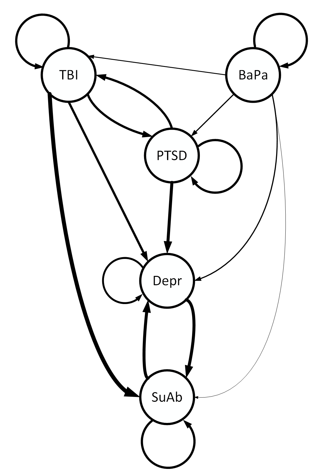
Equation 12 is a convex function in terms of and can be maximized using a convex optimization algorithms such as Newton-Raphson (See Figure 1).
Given the structure of the functional CTBN, i.e. the parent set for each variable, the maximum number of parameters to be estimated in Equation 12 will be , where is the number of state variables (conditions), is the number of exogenous variables (risk factors) presents in the system, and max() is the maximum number of parents considered (pre-existing diseases for each condition). Therefore, as in classical Bayesian networks, the number of parents has a direct and exponential influence on the computational efficiency of the estimation process and should be limited to a small number.
We propose to assume the conditional effect of parents is multiplicative, i.e. , to make the conditional effect of the risk factors additive given the set of parents, i.e. . This assumption , which is on a par with the Noisy-OR [48, 51] and the CT-NOR [49], reduces the maximum number of parameters to be estimated to ). However, in situations where the number of exogenous variables (risk factors for the multiple chronic conditions) are large, the estimation of the Poisson regression parameters can still be computationally challenging, even with the multiplicative assumption. To address this problem, we propose to consider principal component analysis (PCA) or kernel PCA (KPCA) to first extract a few informative features of z, and then use those features of the original covariates for building the Poisson regression model for each conditional intensity [39]. While reducing the interpretability of the estimated parameters (), using dimensionality reduction (PCA or KPCA) helps with efficient modeling of the non/linear relationship among the risk factors. Considering the PCA for our case study, while it is restricted to only linear correlation between (exogenous) variables, Our analysis shows the PCA captures a considerable portion of variation (>82%) in our dataset using only the first principal component, which is also evidenced in the proposed methodology performance as described in Section V.
IV-C Adaptive Group Regularization Framework for Structure Learning in Continuous Time Bayesian Network
The parameter estimation approach presented above requires the parent set of each condition to be known, which is equivalent to knowing the structure of the Bayesian network. Here, we propose an adaptive group regularization-based framework to simultaneously learn the structure () and conditional intensities of the functional Bayesian network model. Regularization-based structure learning is a recent approach that is gaining popularity for parameter estimation in graphical models[40, 41, 42]. However, since regularization can result in cycles in graphical models, it is not generally considered for directed graphs. Given that the proposed functional CTBN has a special structure based on a conditional intensity matrix that allows for cycles, this study proposes to extend the regularization-based structure learning to functional CTBN.
Considering the negative log likelihood of the fully connected functional CTBN, we propose to add an adaptive group regularization term to the negative log likelihood function to penalize groups of parameters pertaining to each specific conditional intensities as in Equation 13.
| (13) |
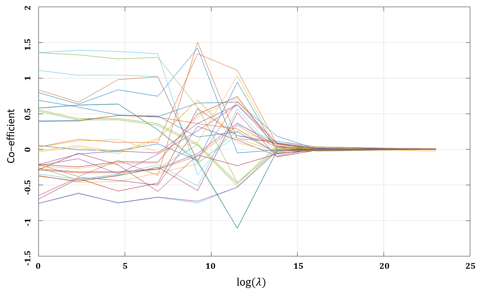
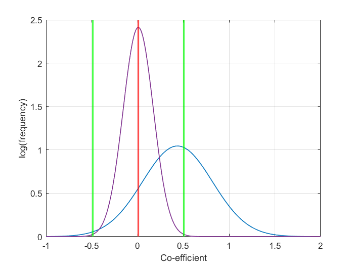
where, is the norm of the group of parameters associated with each conditional intensity, is the groups size which is based on the number of coefficients in the Poisson regression for each conditional intensity, is the tuning parameters of the adaptive group regularization that control the amount of shrinkage, where is inversely weighted based on the unpenalized estimated value of the regression coefficients [43]. The index implies the adaptive penalization applied to each grouped parameter. Fast-iterative shrinkage thresholding algorithm (FISTA) can be used for solving Equations 13 [44]. Figure 3 shows the regularization path of the tuning parameter for some of the parameters of the proposed model.
An interesting feature of the adaptive group-regularization based structure learning is that we can use the regularization path to control the level of sparsity in the proposed functional CTBN (See Figure 2).
IV-D Post Processing and Early Stopping
Each of the conditional dependencies (edges) in the proposed functional CTBN is consisted of a Poisson regressions with multiple exogenous variables. For cases where the number of parent variables and/or the exogenous variables are large, the process of structure and parameter learning requires substantial computation. However, the majority of changes in the estimated values of the (Poisson regression) parameters happen in the early iterations of the learning algorithm. The (numerous) remaining iterations of the learning algorithms make minor adjustments to the estimated values of the parameters, especially pushing parameters with a small value toward zero. These later steps to push insignificant parameters toward zero can take many iterations without significantly changing other (significant) parameter values.
Meanwhile, for a sufficiently large choice of the tuning parameter, some of the parameters will be zero. This is because for a general regression problem, setting the tuning parameter to infinity results in all coefficients except the intercept to be zero. On the other hand, a very small choice of the tuning parameter can result in all estimated parameters being non-zero. Additionally, having all the parameters in the proposed model as non-zero would be equivalent to having a fully connected functional CTBN network, which is not expected in most cases. Therefore, it is plausible to have some zero parameters to be discovered by an appropriate regularization method, such as the adaptive group regularization framework as described in section IV-C.
To reduce the number of (additional) iterations for zeroing non-significant parameters, we propose to use Gaussian mixture models (GMM). For this purpose, we stop the learning algorithm when there is no significant change in the estimated parameters. Next, we use a GMM to model the estimated parameters [45]. The GMM is expected to have one cluster with a mean around zero (representing the insignificant parameters to be pushed toward zero) and one or more clusters with non-zero means (representing significant parameters). Once the clusters and their parameters are identified, we choose the cluster with (around) zero mean and assign a value of zero to all parameters within (standard deviation) around the mean . We run an additional iteration of the learning algorithm with the zerod́ parameters to ensure convergence.
| Sl No. | Race | Gender | Marital Status | Age Group | Education | ||||||||||
|---|---|---|---|---|---|---|---|---|---|---|---|---|---|---|---|
| Male | Female | Married | Un-Married | 18-30 | 31-40 | 41-50 | 51- Rest | Unknown | High School | High School | Some College | College Graduate | Post College | ||
| 1 | White | 148355 | 19183 | 74487 | 93051 | 96799 | 36003 | 26167 | 8569 | 2334 | 2037 | 129921 | 16743 | 12024 | 4479 |
| 57.58% | 7.45% | 28.91% | 36.12% | 37.57% | 13.97% | 10.16% | 3.33% | 0.91% | 0.79% | 50.43% | 6.50% | 4.67% | 1.74% | ||
| 2 | Black | 35758 | 11828 | 23308 | 24278 | 20047 | 12468 | 12710 | 2361 | 658 | 504 | 37506 | 4819 | 3160 | 939 |
| 13.88% | 4.59% | 9.05% | 9.42% | 7.78% | 4.84% | 4.93% | 0.92% | 0.26% | 0.20% | 14.56% | 1.87% | 1.23% | 0.36% | ||
| 3 | Hispanic | 25373 | 4232 | 14523 | 15082 | 17016 | 6606 | 4758 | 1225 | 386 | 360 | 23592 | 2933 | 1893 | 441 |
| 9.85% | 1.64% | 5.64% | 5.85% | 6.60% | 2.56% | 1.85% | 0.48% | 0.15% | 0.14% | 9.16% | 1.14% | 0.73% | 0.17% | ||
| 4 | Asian | 5639 | 981 | 3067 | 3553 | 3235 | 1361 | 1564 | 460 | 131 | 60 | 4732 | 598 | 879 | 220 |
| 2.19% | 0.38% | 1.19% | 1.38% | 1.26% | 0.53% | 0.61% | 0.18% | 0.05% | 0.02% | 1.84% | 0.23% | 0.34% | 0.09% | ||
| 5 | Native | 3081 | 707 | 1747 | 2041 | 2115 | 925 | 564 | 184 | 60 | 60 | 3004 | 376 | 217 | 71 |
| 1.20% | 0.27% | 0.68% | 0.79% | 0.82% | 0.36% | 0.22% | 0.07% | 0.02% | 0.02% | 1.17% | 0.15% | 0.08% | 0.03% | ||
| 6 | Unknown | 2135 | 361 | 1346 | 1150 | 1062 | 625 | 673 | 136 | 51 | 22 | 1808 | 287 | 223 | 105 |
| 0.83% | 0.14% | 0.52% | 0.45% | 0.41% | 0.24% | 0.26% | 0.05% | 0.02% | 0.01% | 0.70% | 0.11% | 0.09% | 0.04% | ||
V Case Study: Identifying Patterns of Multiple Chronic Conditions
Long-lasting diseases, otherwise known as chronic conditions, can be considered a staple example of degradation processes that progress over time and contribute to the development of other new chronic conditions. The presence of two or more chronic medical conditions in an individual is commonly defined as multimorbidity, or multiple chronic conditions (MCC) [46]. Here, we use the proposed functional CTBN to find the impact of patient level risk factors on the conditional dependencies of MCC and the evolution of different chronic conditions over time.
V-A Study Population and Demographics
The proposed case study dataset includes 608,503 patients with two or more MCC (including Traumatic Brain Injury (TBI), Post Traumatic Stress Disorder (PTSD), Depression (Depr), Substance Abuse (SuAb), and Back pain (BaPa)) who received medical care from the Department of Veteran Affairs for at least three years between 2002-2015. For meaningful prediction, we have removed the data for patients whose data was not maintained over three years. The dropout of patient information may be caused by but not limited to death, not requiring care or receiving care, etc. After dropping such data, the number of patients considered for the analysis is 257,633. The dataset includes the ICD-9-CM diagnosis codes documented during the course of VA care, during each inpatient or outpatient encounter. The risk factors (exogenous variables) considered in the dataset include age at VA entry, sex, race/ethnicity (White, African American, Hispanic, Asian/Pacific Islander, Native American, unknown), and education (less than high school, high school graduate, some college, college graduate, post-college education). Table I shows the summary of the collected data based on patients’ demographics. In this study, in order to reduce the computational complexity of the algorithm and to show the application of the dimensionality reduction technique, we use PCA to reduce the number of risk factors into one.
V-B Diagnosed Health Conditions
We used ICD-9-CM codes from the inpatient and outpatient data (excluding ancillary and telephone care) to identify Traumatic brain injury (TBI), Post Traumatic Disorder (PTSD), Depression (Depr), substance abuse (SuAb), Back pain (BaPa) using validated published algorithms [47]. PTSD, SuAb, and BaPa required two diagnoses at least seven days apart, while TBI, which is an acute injury, required only a single diagnosis. Each condition was coded as “0” or “1” for each year of care, with 1 indicating a diagnosis for that condition regardless of the number of instances for which each condition was diagnosed (Additional information on ICD-9 codes for the considered conditions can be found on appendix B).

V-C Structure and Parameter Learning
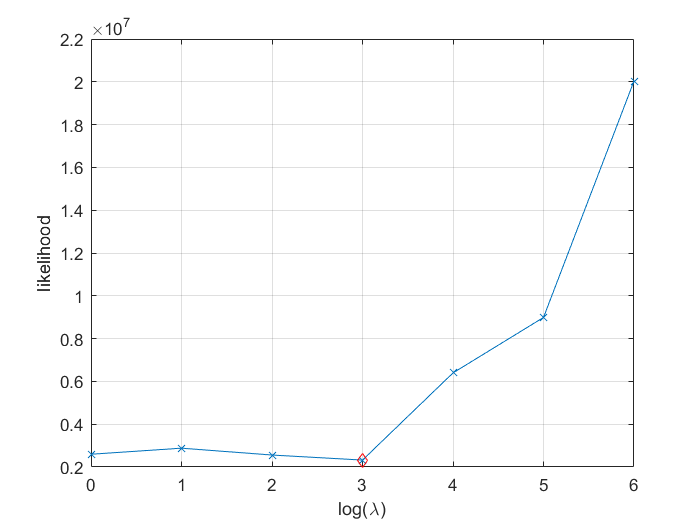
To identify the optimal value of the tuning parameter () of the group regularization method for structure and parameter learning, we use cross-validation error based on several values (). Figure 4a shows the cross-validation error for different values.
We attain the structure of the functional CTBN and the conditional intensities based on the parameters estimated using the optimal value of . Figure 4c illustrates the heatmap of the estimated parameters () of the proposed CTBN based on . As shown in figure 4a and 4c, setting not only provides considerably low (cross validation) error, but also significantly reduces the number of (non zero) parameters (a sparsity ratio of 64.75%).
Figure 4c provides the heatmap of the estimated parameters of the learned functional CTBN model, which is equivalent to the graphical model presented in figure 1. To identify the final structure of the functional CTBN, considering the sparse learned parameter matrix in figure 4c, if all parameters (coefficients) of the Poisson regression connecting a parent node to a child node are zero, there exists no edge between them. On the other hand, if there exists a non zero parameter for the Poisson regression model connecting a parent node to a child node, there exists an edge between the two nodes, where the strength of the connection is represented by the conditional intensity value.
Meanwhile, to reduce the number of training iterations for obtaining the spare matrix in Figure 4c, we use GMM as explained in section IV-D. Figure 4b shows the Gaussian densities fitted to the estimated parameters at iteration 30,000 of the learning algorithm, which shows two clusters including one with zero mean and small variation (non significant parameters), and the other with non zero mean and high variance (significant parameters). We assign a value of zero to all parameters within (standard deviation) of the cluster with the mean around zero. We have verified this result by running the learning algorithm for an additional 20,000 iterations.
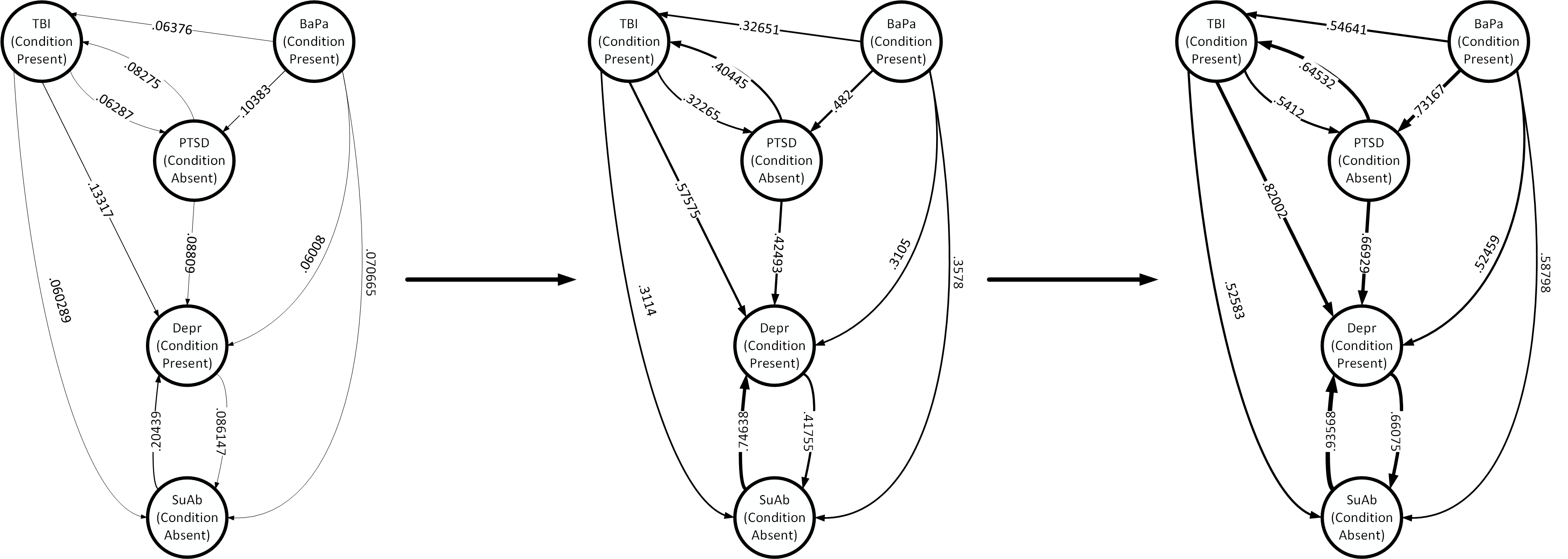
Additionally, the functional CTBN allows for loop in the structure (as shown in figure 1). This is an important feature in studying MCC, because an MCC condition can simultaneously be the cause and/or the effect (result) of another MCC condition, i.e., depression and substance abuse. The functional CTBN also allows for the self-loops to represent staying in the same MCC state (existing/parent conditions) over (fixed amount of) time [19].
Figure 5 illustrates the dynamics of the transition probabilities of MCC, namely the risk of acquiring a new condition over a period of three years for a sample patient with preexisting conditions TBI, BaPa, and Depression. As shown in the figure, the transition probabilities change as a function of time, which is intuitive in the presence of the preexisting conditions TBI, BaPa, and Depression. In particular, having the preexisting conditions TBI, BaPa, and Depression increases the likelihood of acquiring the new disorders PTSD and SuAb over time. It also increases the reinforcing loop between the existing conditions, which is also intuitive. This can help health practitioners and patients to better the short- and long-term (negative) impact of MCC on acquiring new conditions.
| Depression | Substance Abuse | PTSD | Back Pain | TBI | |||||||||||
| FCTBN | MTBN | LRMCL | FCTBN | MTBN | LRMCL | FCTBN | MTBN | LRMCL | FCTBN | MTBN | LRMCL | FCTBN | MTBN | LRMCL | |
| Year 2 | 75.89% | 66.92% | 67.34% | 76.61% | 72.09% | 71.91% | 79.72% | 78.31% | 67.02% | 73.53% | 64.28% | 66.35% | 65.72% | 72.11% | 67.59% |
| Year 3 | 70.98% | 65.96% | 56.12% | 72.34% | 69.09% | 59.54% | 75.75% | 74.95% | 63.88% | 69.65% | 62.16% | 56.48% | 63.36% | 70.08% | 57.03% |
| Year 4 | 68.92% | 64.70% | 49.61% | 70.75% | 68.02% | 53.00% | 73.76% | 73.36% | 62.25% | 67.79% | 55.32% | 50.18% | 63.33% | 69.19% | 51.02% |
| Year 5 | 67.40% | 64.11% | 46.44% | 69.54% | 59.41% | 42.87% | 72.38% | 71.92% | 61.18% | 66.57% | 62.66% | 48.08% | 62.92% | 69.56% | 49.21% |
V-D Performance Evaluation: Predictive Power
We utilize the validation set method based on 250 000 patients for training and 7 633 patients for validation, along with the Area Under the Curve (AUC) of the receiver Operatic Characteristic (ROC) function to evaluate the performance of the proposed FCTBN model. We also compare the performance of the FCTBN with two existing methods from the literature including unsupervised MTBN [4] and LRMCL[19]. The step-by-step procedure of training and testing of the comparing algorithms is provided in appendix A. For the comparisons, considering the patients’ existing MCC in the base year, which can be any combination of the 5 MCC including no condition, we use each of the comparing methods to predict the future combination of conditions for the next 5 years.
Table II illustrates the AUC performance of the comparing methods for each of the five conditions (presented in the columns) for 2 to 5 years from the baseline (presented in the rows). As can be seen from the table, the proposed functional CTBN generally provides better accuracy compared to MTBN and LRMCL for 4 out or the 5 conditions (Depression, Substance Abuse, PTSD, and Backpain) over both short and long term predictions (2-5 years). However, it shows less predictive power compared to MTBN for forecasting TBI. One justification for the lower prediction accuracy for TBI may be the distinct temporal behavior of TBI occurrences. At the patient level, TBI occurrence is generally a more singular event with chronic clinical ramifications that are coded separately in the electronic medical record. Meanwhile, the performance gap improves for the longer predictions, i.e., years 4 and 5, as it captures the temporal pattern of staying in the TBI state more effectively.
It may also be worth noting that the predictive performance of the functional CTBN as shown in Table II is based on the model trained on risk factors with reduced dimension (1st principal component of the risk factors) to improve the computational time, while the MTBN and LRMCL take advantage of the original risk factors. Therefore, we believe training the functional CTBN model with the complete risk factors may further enhance its predictive performance (with the trade-off of increasing the computational time).
We believe the improved performance of the functional CTBN is partly because of the proposed adaptive group regularization-based learning framework for structure and parameter learning. Specifically, we believe the use of group regularization, in the way proposed in the manuscript, results in fewer yet more informative connections, which improve the training and querying (inference) process. We have shown this concept in one of our related research works [66]. We also believe allowing the model to contain loops (bidirectional connections) helps better capturing the (reinforcing) dynamics of the multiple chronic conditions. Additionally, we think explicit capturing of the time can positively affect the learning of parameters of the model, even though the prediction task is actually on discrete time stamps, i.e., years.
V-E Trajectory Analysis
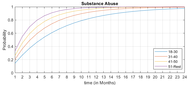
An interesting feature of the proposed functional CTBN is the trajectory analysis of state variables (MCC conditions). Here, we demonstrate two cases of MCC trajectory analyses for different preexisting (parent) conditions and age groups (exogenous variables). In the first case, we investigate the effect of age (groups) on the trajectory of Substance Abuse given TBI and PTSD as the preexisting conditions. Figure 6 shows the most probable trajectory for the emergence of substance abuse for different age groups for the next 24 months given TBI and PTSD in the base month. It can be seen that the above 51 age group is more prone to be diagnosed with substance abuse than younger age groups, with the probability of developing substance abuse for this age group goes above 80% just after four months. Whereas, the 18-30 age group reaches 80% after 10 months, the 31-40 age group passes 80% mark after 7 months, and the 41-50 group meets the 80% mark after 5 months.
This is on par with findings in the medical literature. In a study with service members with mild TBI Miller et al. [59] found an increased risk for addiction-related disorders including alcohol and nicotine. In a separate study with 6,824 military personnel, Adams et al. [60] conducted a path based analysis to examine the association of binge alcohol drinking with TBI and PTSD. They found almost 70% of the total effect of TBI on binge drinking was from the direct path effect, and only 30% represented the indirect effect through PTSD. Graham et al. [65] found a decrease in substance abuse post-TBI in a younger age group, likely motivated by significant influences on lifestyle choices and functional status given proper support from VA.
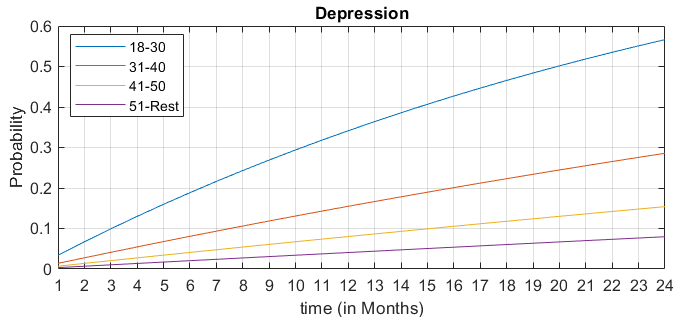
In the second case, we investigate the effect of age (groups) on the trajectory of depression given PTSD as the existing (prior) conditions. Figure 7 shows the most probable trajectory for the emergence of depression for different age groups for the next 24 months given PTSD in the base month. As can be seen from figure 7 the probability of developing depression after PTSD increases (almost) linearly over time, but with a different slope for different age groups. Unlike the first case, here, the younger patients, i.e., 18-30 age group, are more like to develop depression compared to the other age groups. As the (blue) trajectory line in figure 7 shows, the 18-30 age group trajectory has a considerably high slope reaching a risk of 50% after 20 months. Meanwhile, the slope of the trajectory line reduces for older age groups, i.e., the purple line in the figure shows a marginal increase in the risk of depression for patients aged 51 and older. These differences in age group findings may reflect variability in clinical screening approaches, provider biases, and differences in clinical priorities by these patient populations, resulting in increased or decreased likelihood of getting diagnosed with these conditions. For example, younger age group veterans have been undergoing a widespread national screening program to identify PTSD and to establish treatment and follow-up, which would likely lead to the additional diagnosis of depression, a known comorbid condition.
The medical literature also supports this result. Lippa et al. [61] used factor analysis to identify patterns of comorbidity in a sample of 255 previously deployed Post-9/11 service members and veterans who participated in a structured clinical interview. They found that over 90% of the patients had psychiatric conditions, and approximately half had three or more conditions. They also identified four clinically relevant psychiatric and behavioral factors, including deployment trauma factor, somatic factor, anxiety factor, and substance abuse factor, which account for 76.9% of the variance in the data. They concluded that depression, PTSD, and a history of military mild TBI could comprise a harmful combination associated with a high risk for substantial disability. In a separate study, Duncan et al. [62] found 36% of depressed patients screened positive for PTSD. Kobayashi et al. [63] found that younger and middle‐aged VA primary care patients had more severe PTSD symptoms compared to older patients; however, it was impossible to disentangle the effects of age from a passage of time, limiting interpretation of the findings. On a separate study, on average, women reported age of onset of the depression of 23 –24 years. About half the women were experiencing a mild-to-moderate depressive episode, with 47% experiencing a severe depressive episode [64]. Such information can help the medical practitioners develop more individualized plans to prevent the emergence of new chronic conditions according to the patient’s specific risk factors and prior conditions.
VI Conclusion
In this paper, we propose a functional continuous time Bayesian network with conditional dependencies represented by regularized Poisson Regression that can be used to learn both the structure and parameters of the network by solving a non-smooth convex optimization problem. While most Bayesian model structures are sensitive to time granularity since the proposed functional CTBN model can model finite-state continuous time Markov processes over a set of factored states at various time granularity. The model incorporates the functional dependencies among random variables in the Bayesian network structure. It allows for extracting the probability distribution of various combinations of events at different times with respect to any predetermined values of exogenous variables. The model also utilizes an adaptive group regularization method to learn a sparse representation of the system. For the case study, we have used the proposed CTBN to model the complex temporal relationship among multiple chronic conditions with respect to patient-level risk factors based on a dataset from the Department of Veterans Affairs.
The proposed model provides a considerable improvement in prediction performance in comparison to Multilevel Temporal Bayesian networks and Latent Regression Markov Mixture Clustering (LRMCL). It also effectively characterizes the trajectory of a medical condition over time when given a different set of starting conditions and risk factors. This approach allows for the personalization of the predictive model and therefore has both population and patient-level applications. This modeling approach will inform the clinician about the emergence trajectory of MCC over time and the significant risk factors affecting the trajectory and help guide clinical care to prevent or delay the onset of new chronic conditions.
References
- [1] J. Pearl and T. S. Verma, “A theory of inferred causation,” in Studies in Logic and the Foundations of Mathematics, ser. Logic, Methodology and Philosophy of Science IX, D. Prawitz, B. Skyrms, and D. Westerståhl, Eds. Elsevier, Jan. 1995, vol. 134, pp. 789–811. [Online]. Available: http://www.sciencedirect.com/science/article/pii/S0049237X06800741
- [2] D. Heckerman, “A Tutorial on Learning with Bayesian Networks,” in Learning in Graphical Models, ser. NATO ASI Series, M. I. Jordan, Ed. Dordrecht: Springer Netherlands, 1998, pp. 301–354. [Online]. Available: https://doi.org/10.1007/978-94-011-5014-9_11
- [3] S. Yang, T. Khot, K. Kersting, and S. Natarajan, “Learning continuous-time bayesian networks in relational domains: A non-parametric approach,” in Thirtieth AAAI Conference on Artificial Intelligence, 2016.
- [4] S. H. A. Faruqui, A. Alaeddini, C. A. Jaramillo, J. S. Potter, and M. J. Pugh, “Mining patterns of comorbidity evolution in patients with multiple chronic conditions using unsupervised multi-level temporal Bayesian network,” PLOS ONE, vol. 13, no. 7, p. e0199768, Jul. 2018. [Online]. Available: https://journals.plos.org/plosone/article?id=10.1371/journal.pone.0199768
- [5] M. Lappenschaar, A. Hommersom, P. J. Lucas, J. Lagro, S. Visscher, J. C. Korevaar, and F. G. Schellevis, “Multilevel temporal bayesian networks can model longitudinal change in multimorbidity,” Journal of clinical epidemiology, vol. 66, no. 12, pp. 1405–1416, 2013.
- [6] K. Kanazawa, “A logic and time nets for probabilistic inference.” in AAAI, 1991, pp. 360–365.
- [7] C. F. Aliferis and G. F. Cooper, “A structurally and temporally extended bayesian belief network model: definitions, properties, and modeling techniques,” in Proceedings of the Twelfth international conference on Uncertainty in artificial intelligence. Morgan Kaufmann Publishers Inc., 1996, pp. 28–39.
- [8] P. KEVIN, “Dynamic Bayesian Networks : Representation, Inference and Learning,” PhD thesis, University of California, 2002. [Online]. Available: https://ci.nii.ac.jp/naid/10014940570/
- [9] T. Dean and K. Kanazawa, “A model for reasoning about persistence and causation,” Computational Intelligence, vol. 5, no. 2, pp. 142–150, 1989. [Online]. Available: https://onlinelibrary.wiley.com/doi/abs/10.1111/j.1467-8640.1989.tb00324.x
- [10] P. Dagum, A. Galper, and E. Horvitz, “Dynamic network models for forecasting,” in Proceedings of the eighth international conference on uncertainty in artificial intelligence. Morgan Kaufmann Publishers Inc., 1992, pp. 41–48.
- [11] G. Arroyo-Figueroa and L. E. Sucar, “A temporal bayesian network for diagnosis and prediction,” in Proceedings of the Fifteenth conference on Uncertainty in artificial intelligence. Morgan Kaufmann Publishers Inc., 1999, pp. 13–20.
- [12] G. ArroyoFigueroa and L. E. Sucar, “Temporal bayesian network of events for diagnosis and prediction in dynamic domains,” Applied Intelligence, vol. 23, no. 2, pp. 77–86, 2005.
- [13] U. Nodelman, C. R. Shelton, and D. Koller, “Learning continuous time bayesian networks,” in Proceedings of the Nineteenth conference on Uncertainty in Artificial Intelligence. Morgan Kaufmann Publishers Inc., 2002, pp. 451–458.
- [14] C. Shaunak and R. Stuart, “Why are DBNs sparse?,” Proceedings of the Thirteenth International Conference on Artificial Intelligence and Statistics, pp. 81–88, 2010
- [15] C. Wang, D. Blei and D. Heckerman, “Continuous time dynamic topic models,” arXiv preprint arXiv:1206.3298, 2012
- [16] U. Nodelman C. R. Shelton, and D. Koller “Continuous Time Bayesian Networks,” in Proceedings of the Eighteenth Conference on Uncertainty in Artificial Intelligence, ser. UAI’02. San Francisco, CA, USA: Morgan Kaufmann Publishers Inc., 2002, pp. 378–387. [Online]. Available: http://dl.acm.org/citation.cfm?id=2073876.2073921
- [17] T. El-Hay, N. Friedman, D. Koller, and R. Kupferman, “Continuous time markov networks,” arXiv preprint arXiv:1206.6838, 2012.
- [18] D. M. Chickering, D. Heckerman, and C. Meek, “Large-sample learning of bayesian networks is np-hard,” Journal of Machine Learning Research, vol. 5, no. Oct, pp. 1287–1330, 2004.
- [19] A. Alaeddini, C. A. Jaramillo, S. H. A. Faruqui, and M. J. Pugh, “Mining Major Transitions of Chronic Conditions in Patients with Multiple Chronic Conditions,” Methods Inf Med, vol. 56, no. 5, pp. 391–400, 2017. [Online]. Available: http://www.thieme-connect.de/DOI/DOI?10.3414/ME16-01-0135
- [20] J. R. Norris, Markov chains. Cambridge university press, 1998, no. 2.
- [21] Y. Fan and C. R. Shelton, “Learning continuous-time social network dynamics,” arXiv preprint arXiv:1205.2648, 2012.
- [22] J. Xu and C. R. Shelton, “Intrusion detection using continuous time bayesian networks,” Journal of Artificial Intelligence Research, vol. 39, pp. 745–774, 2010.
- [23] D. Shi, X. Tang, and J. You, “An intelligent system based on adaptive ctbn for uncertainty reasoning in sensor networks,” Intelligent Automation & Soft Computing, vol. 16, no. 3, pp. 337–351, 2010.
- [24] H. Boudali and J. B. Dugan, “A continuous-time bayesian network reliability modeling, and analysis framework,” IEEE transactions on reliability, vol. 55, no. 1, pp. 86–97, 2006.
- [25] B. Ng, A. Pfeffer, and R. Dearden, “Continuous time particle filtering,” in International joint conference on artificial intelligence, vol. 19. Citeseer, 2005, p. 1360.
- [26] E. Gatti, D. Luciani, and F. Stella, “A continuous time bayesian network model for cardiogenic heart failure,” Flexible Services and Manufacturing Journal, vol. 24, no. 4, pp. 496–515, 2012.
- [27] U. Nodelman, C. R. Shelton, and D. Koller, “Expectation maximization and complex duration distributions for continuous time bayesian networks,” arXiv preprint arXiv:1207.1402, 2012.
- [28] D. Codecasa and F. Stella, “Conditional log-likelihood for continuous time bayesian network classifiers,” in International workshop NFMCP held at ECML-PKDD, vol. 2013, 2013.
- [29] L. Perreault and J. Sheppard, “Compact structures for continuous time bayesian networks,” International Journal of Approximate Reasoning, vol. 109, pp. 19–41, 2019.
- [30] L. Sturlaugson and J. W. Sheppard, “Inference complexity in continuous time bayesian networks.” in UAI. Citeseer, 2014, pp. 772–779.
- [31] Y. Fan, J. Xu, and C. R. Shelton, “Importance sampling for continuous time bayesian networks,” Journal of Machine Learning Research, vol. 11, no. Aug, pp. 2115–2140, 2010.
- [32] U. Nodelman, D. Koller, and C. R. Shelton, “Expectation propagation for continuous time bayesian networks,” arXiv preprint arXiv:1207.1401, 2012.
- [33] S. Saria, U. Nodelman, and D. Koller, “Reasoning at the right time granularity,” arXiv preprint arXiv:1206.5260, 2012.
- [34] T. El-Hay, N. Friedman, and R. Kupferman, “Gibbs sampling in factorized continuous-time markov processes,” arXiv preprint arXiv:1206.3251, 2012.
- [35] Y. Fan and C. R. Shelton, “Sampling for approximate inference in continuous time bayesian networks.” in ISAIM, 2008.
- [36] T. El-Hay, I. Cohn, N. Friedman, and R. Kupferman, “Continuous-time belief propagation.” in ICML, 2010, pp. 343–350.
- [37] I. Cohn, T. El-Hay, N. Friedman, and R. Kupferman, “Mean field variational approximation for continuous-time bayesian networks,” Journal of Machine Learning Research, vol. 11, no. Oct, pp. 2745–2783, 2010.
- [38] C. R. Shelton, Y. Fan, W. Lam, J. Lee, and J. Xu, “Continuous time bayesian network reasoning and learning engine,” Journal of Machine Learning Research, vol. 11, no. Mar, pp. 1137–1140, 2010.
- [39] A. Alaeddini, D. J. E. Helm, D. P. Shi, and S. H. A. Faruqui, “An integrated framework for reducing hospital readmissions using risk trajectories characterization and discharge timing optimization,” IISE Transactions on Healthcare Systems Engineering, no. just-accepted, pp. 1–26, 2019.
- [40] S.-I. Lee, V. Ganapathi, and D. Koller, “Efficient structure learning of markov networks using -regularization,” in Advances in neural Information processing systems, 2007, pp. 817–824.
- [41] M. J. Wainwright, J. D. Lafferty, and P. K. Ravikumar, “High-dimensional graphical model selection using -regularized logistic regression,” in Advances in neural information processing systems, 2007, pp. 1465–1472.
- [42] M. Schmidt, A. Niculescu-Mizil, K. Murphy et al., “Learning graphical model structure using l1-regularization paths,” in AAAI, vol. 7, 2007, pp. 1278–1283.
- [43] H. Wang and C. Leng, ”A note on adaptive group lasso,” Computational Statistics & Data Analysis, vol. 52, pp. 5277–5286, 2008.
- [44] A. Alaeddini and S. H. Hong, “A multi-way multi-task learning approach for multinomial logistic regression,” Methods of information in medicine, vol. 56, no. 04, pp. 294–307, 2017.
- [45] G. McLachlan and D. Peel, “Finite mixture models john wiley & sons,” Inc. Hoboken, New Jersey, 2000.
- [46] E. Wallace, C. Salisbury, B. Guthrie, C. Lewis, T. Fahey, and S. M. Smith, “Managing patients with multimorbidity in primary care,” BMJ, vol. 350, p. h176, Jan. 2015. [Online]. Available: https://www.bmj.com/content/350/bmj.h176
- [47] AJ. Selim, B.G. Fincke, X.S. Ren, A. Lee, W.H. Lee, H. William, D.R. Miller, M. Katherine, M. Linzer and L. Kazis, “Comorbidity assessments based on patient report: results from the Veterans Health Study”, The Journal of ambulatory care management, vol. 27, no. 03, pp. 281–295, 2004.
- [48] J. Pearl, “Probabilistic Reasoning in Intelligent Systems: Networks of Plausible Inference,” Morgan Kaufmann, 1988
- [49] A. Simma, M. Goldszmidt, J. MacCormick, P. Barham, R. Black, R. Isaacs, and R. Mortier, “CT-NOR: representing and reasoning about events in continuous time”. In Proceedings of the Twenty-Fourth Conference on Uncertainty in Artificial Intelligence, (UAI’08). AUAI Press, Arlington, Virginia, USA, 484–493.
- [50] L. Perreault, S. Strasser, M. Thornton, and J. Sheppard, “A noisy-or model for continuous time Bayesian networks”,In The Twenty-Ninth International Flairs Conference, 2016.
- [51] A. Onisko, M.J. Druzdzel, and H. Wasyluk, “Learning Bayesian network parameters from small data sets: Application of noisy-or gates,” International Journal of Approximate Reasoning, 27(2):165–182, 2001.
- [52] D. Cao, “Novel models and algorithms for systems reliability modeling and optimization”, Ph.D. Dissertation, Wayne State University, 2011.
- [53] A. Gunawardana and C. Meek, “Universal models of multivariate temporal point processes,” In Artificial Intelligence and Statistics, pp. 556-563. PMLR, 2016.
- [54] A. Simma and M. I. Jordan, “Modeling events with cascades of Poisson processes,” arXiv preprint arXiv:1203.3516.
- [55] S. Rajaram, T. Graepel and R. Herbrich, “Poisson-networks: A model for structured point processes,” In Proceedings of the 10th international workshop on artificial intelligence and statistics, pp. 277-284. 2005.
- [56] W. Truccolo, U.T. Eden, M.R. Fellows, J.P. Donoghue, and E. N. Brown, “A point process framework for relating neural spiking activity to spiking history, neural ensemble, and extrinsic covariate effects,” Journal of neurophysiology, 93(2), 1074-1089, 2005.
- [57] S. Srinivas, “A generalization of the noisy-or model,” In Uncertainty in artificial intelligence, pp. 208-215. Morgan Kaufmann, 1993.
- [58] M. Henrion, “Practical issues in constructing belief networks,” In Proceedings of the Third Conference on Uncertainty in Artificial Intelligence, Corvallis, OR: AUAI Press, 1989.
- [59] SC. Miller, SH. Baktash, TS. Webb, CR. Whitehead, C. Maynard, TS. Wells, “Risk for Addiction-Related Disorders Following Mild Traumatic brain injury in a Large Cohort of Active-Duty U.S. Airmen,” American Journal of Psychiatry, Apr 1;170(4):383–90, 2013.
- [60] RS. Adams, MJ. Larson, JD. Corrigan, GA. Ritter, CM. Horgan, RM. Bray, TV. Williams, “Combat acquired traumatic brain injury, posttraumatic stress disorder, and their relative associations with postdeployment binge drinking,” Journal of Head Trauma Rehabilitation, 31(1):13–22, 2016
- [61] SM. Lippa, JR. Fonda, CB. Fortier, MA. Amick, A. Kenna, WP. Milberg, “Deployment Related Psychiatric and Behavioral Conditions and Their Association with Functional Disability in OEF/OIF/OND Veterans,” Journal of traumatic stress, 28(1):25, 2015.
- [62] DG. Campbell, BL. Felker, CF. Liu, EM. Yano, JE. Kirchner, D. Chan, LV. Rubenstein, EF. Chaney, “Prevalence of depression–PTSD comorbidity: Implications for clinical practice guidelines and primary care-based interventions,” Journal of general internal medicine, Jun 1;22(6):711-8, 2007.
- [63] I. Kobayashi, J.M. Boarts,, D.L. Delahanty “Polysomnographically measured sleep abnormalities in PTSD: A meta‐analytic review,” Psychophysiology, 44(4), 660-669, 2007.
- [64] B.K. Green, J.L. krupnick, J. Chung, J. Siddique, E.D. Krause, D. Revicki, L. Frank, J. Miranda, “Impact of PTSD comorbidity on one‐year outcomes in a depression trial,” Journal of clinical psychology, 62(7), 815-835, 2006.
- [65] D.P. Graham, A.L. Cardon, “An update on substance use and treatment following traumatic brain injury,” Annals of the New York Academy of Sciences, 1141(1), 148-162, 2008.
- [66] S.H.A. Faruqui. A. Alaeddini, M. Chang, S. Shirinkam, C. Jaramillo, P. Najafirad, J. Wang, M.J. Pugh, “Summarizing Complex Graphical Models of Multiple Chronic Conditions Using the Second Eigenvalue of Graph Laplacian: Algorithm Development and Validation,” JMIR medical informatics, 8(6), e16372, 2020.