Deep direct likelihood knockoffs

Abstract

Predictive modeling often uses black box machine learning methods, such as deep neural networks, to achieve state-of-the-art performance. In scientific domains, the scientist often wishes to discover which features are actually important for making the predictions. These discoveries may lead to costly follow-up experiments and as such it is important that the error rate on discoveries is not too high. Model-X knockoffs [2] enable important features to be discovered with control of the false discovery rate (fdr). However, knockoffs require rich generative models capable of accurately modeling the knockoff features while ensuring they obey the so-called “swap” property. We develop Deep Direct Likelihood Knockoffs (ddlk), which directly minimizes the ${\mathrm{KL}}$ divergence implied by the knockoff swap property. ddlk consists of two stages: it first maximizes the explicit likelihood of the features, then minimizes the ${\mathrm{KL}}$ divergence between the joint distribution of features and knockoffs and any swap between them. To ensure that the generated knockoffs are valid under any possible swap, ddlk uses the Gumbel-Softmax trick to optimize the knockoff generator under the worst-case swap. We find ddlk has higher power than baselines while controlling the false discovery rate on a variety of synthetic and real benchmarks including a task involving a large dataset from one of the epicenters of COVID-19.

1 Introduction

High dimensional multivariate datasets pervade many disciplines including biology, neuroscience, and medicine. In these disciplines, a core question is which variables are important to predict the phenomenon being observed. Finite data and noisy observations make finding informative variables impossible without some error rate. Scientists therefore seek to find informative variables subject to a specific tolerance on an error rate such as the false discovery rate (fdr).

Traditional methods to control to the fdr rely on assumptions on how the covariates of interest ${\mathbf{x}}$ may be related to the response ${\mathbf{y}}$. Model-X knockoffs [2] provide an alternative framework that controls the fdr by constructing synthetic variables ${\widetilde{\mathbf{x}}}$, called knockoffs, that look like the original covariates, but have no relationship with the response given the original covariates. Variables of this form can be used to test the conditional independence of each covariate in a collection, with the response given the rest of the covariates by comparing the association the original covariate has with the response with the association the knockoff has with the response.

The focus on modeling the covariates shifts the testing burden to building good generative models of the covariates. Knockoffs need to satisfy two properties: (i) they need to be independent of the response given the real covariates, (ii) they need to be equal in distribution when any subset of variables is swapped between knockoffs and real data. Satisfying the first property is trivial by generating the knockoffs without looking using the response. The second property requires building conditional generative models that are able to match the distribution of the covariates.

Related work.

Existing knockoff generation methods can be broadly classified as either model-specific or flexible. Model-specific methods such as hidden markov models (hmms) [22] or Auto-Encoding Knockoffs [15] make assumptions about the covariate distribution, which can be problematic if the data does not satisfy these assumptions. Hmms assume the joint distribution of the covariates can be factorized into a markov chain. Auto-Encoding Knockoffs use variational auto-encoders (vaes) to model ${\mathbf{x}}$ and sample knockoffs ${\widetilde{\mathbf{x}}}$. Vaes assume ${\mathbf{x}}$ lies near a low dimensional manifold, whose dimension is controlled by a latent variable. Covariates that violate this low-dimensional assumption can be better modeled by increasing the dimension of the latent variable, but risk retaining more information about ${\mathbf{x}}$, which can reduce the power to select important variables.

Flexible methods for generating knockoffs such as KnockoffGAN [10] or Deep Knockoffs [20] focus on likelihood-free generative models. KnockoffGAN uses generative adversarial network (gan)-based generative models, which can be difficult to estimate [18] and sensitive to hyperparameters [21, 8, 17]. Deep Knockoffs employ maximum mean discrepancys (mmds), the effectiveness of which often depends on the choice of a kernel which can involve selecting a bandwidth hyperparameter. Ramdas et al. [19] show that in several cases, across many choices of bandwidth, mmd approaches 0 as dimensionality increases while ${\mathrm{KL}}$ divergence remains non-zero, suggesting mmds may not reliably generate high-dimensional knockoffs. Deep Knockoffs also prevent the knockoff generator from memorizing the covariates by explicitly controlling the correlation between the knockoffs and covariates. This is specific to second order moments, and may ignore higher order ones present in the data.

We propose deep direct likelihood knockoffs (ddlk), a likelihood-based method for generating knockoffs without the use of latent variables. Ddlk is a two stage algorithm. The first stage uses maximum likelihood to estimate the distribution of the covariates from observed data. The second stage estimates the knockoff distribution with likelihoods by minimizing the Kullback–Leibler divergence (kl) between the joint distribution of the real covariates with knockoffs and the joint distribution of any swap of coordinates between covariates and knockoffs. Ddlk expresses the likelihoods for swaps in terms of the original joint distribution with real covariates swapped with knockoffs. Through the Gumbel-Softmax trick [9, 16], we optimize the knockoff distribution under the worst swaps. By ensuring that the knockoffs are valid in the worst cases, ddlk learns valid knockoffs in all cases. To prevent ddlk from memorizing covariates, we introduce a regularizer to encourage high conditional entropy for the knockoffs given the covariates. We study ddlk on synthetic, semi-synthetic, and real datasets. Across each study, ddlk controls the fdr while achieving higher power than competing gan-based, mmd-based, and autoencoder-based methods.

2 Knockoff filters

Model-X knockoffs [2] is a tool used to build variable selection methods. Specifically, it facilitates the control of the fdr, which is the proportion of selected variables that are not important. In this section, we review the requirements to build variable selection methods using Model-X knockoffs.

Consider a data generating distribution $q({\mathbf{x}})q({\mathbf{y}}\mid{\mathbf{x}})$ where variables ${\mathbf{x}}\in\mathbb{R}^{d}$, response ${\mathbf{y}}$ only depends on ${\mathbf{x}}_{S}$, $S\subseteq[d]$, and ${\mathbf{x}}_{S}$ is a subset of the variables. Let $\hat{S}$ be a set of indices identified by a variable selection algorithm. The goal of such algorithms is to return an $\hat{S}$ that maximizes the number of indices in $S$ while maintaining the fdr at some nominal level:

$$\text{\lx@glossaries@gls@link{acronym}{fdr}{\leavevmode{fdr}}}=\mathbb{E}\left[\frac{|\{j:j\in\hat{S}\setminus S\}|}{\max\left(|\{j:j\in\hat{S}\}|,1\right)}\right].$$

To control the fdr at the nominal level, Model-X knockoffs requires (a) knockoffs ${\widetilde{\mathbf{x}}}$, and (b) a knockoff statistic $w_{j}$ to assess the importance of each feature ${\mathbf{x}}_{j}$.

Knockoffs ${\widetilde{\mathbf{x}}}$ are random vectors that satisfy the following properties for any set of indices $H\subseteq[d]$:

$$[{\mathbf{x}},{\widetilde{\mathbf{x}}}] \overset{d}{=}[{\mathbf{x}},{\widetilde{\mathbf{x}}}]_{\text{swap}(H)}$$ (1)

$${\mathbf{y}} \perp{\widetilde{\mathbf{x}}}\mid{\mathbf{x}}.$$ (2)

The swap property eq. 1 ensures that the joint distribution of $[{\mathbf{x}},{\widetilde{\mathbf{x}}}]$ is invariant under any swap. A swap operation at position $j$ is defined as exchanging the entry of ${\mathbf{x}}_{j}$ and ${\widetilde{\mathbf{x}}}_{j}$. For example, when ${\mathbf{x}}=[{\mathbf{x}}_{1},{\mathbf{x}}_{2},{\mathbf{x}}_{3}]$, and $H=\{1,3\}$, $[{\mathbf{x}},{\widetilde{\mathbf{x}}}]_{\text{swap}(H)}=[{\widetilde{\mathbf{x}}}_{1},{\mathbf{x}}_{2},{\widetilde{\mathbf{x}}}_{3},{\mathbf{x}}_{1},{\widetilde{\mathbf{x}}}_{2},{\mathbf{x}}_{3}]$. Equation 2 ensures that the response ${\mathbf{y}}$ is independent of the knockoff ${\widetilde{\mathbf{x}}}$ given the original features ${\mathbf{x}}$.

A knockoff statistic $w_{j}$ must satisfy the flip-sign property. This means if ${\mathbf{x}}_{j}\in S$, $w_{j}$ must be positive. Otherwise, the sign of $w_{j}$ must be positive or negative with equal probability.

Given knockoff ${\widetilde{\mathbf{x}}}$ and knockoff statistics $\{w_{j}\}_{j=1}^{d}$, exact control of the fdr at level $p$ can be obtained by selecting variables in ${\mathbf{x}}$ such that $w_{j}>\tau_{p}$. The threshold $\tau_{p}$ is given by:

$$\tau_{p}=\underset{t>0}{\min}\left\{t:\frac{1+|\{j:w_{j}\leq-t\}|}{|\{j:w_{j}\geq t\}|}\leq p\right\}.$$ (3)

While knockoffs are a powerful tool to ensure that the fdr is controlled at the nominal level, the choice of method to generate knockoffs is left to the practitioner.

Existing methods for knockoffs include model-specific approaches that make specific assumptions about the covariate distribution, and flexible likelihood-free methods. If the joint distribution of ${\mathbf{x}}$ cannot be factorized into a markov chain [22] or if ${\mathbf{x}}$ does not lie near a low-dimensional manifold [15], model-specific generators will yield knockoffs that are not guaranteed to control the fdr. Likelihood-free generation methods that use gans [10] or mmds [20] make fewer assumptions about ${\widetilde{\mathbf{x}}}$, but can be difficult to estimate [18], sensitive to hyperparameters [21, 8, 17], or suffer from low power in high dimensions [19]. In realistic datasets, where ${\mathbf{x}}$ can come from an arbitrary distribution and dimensionality is high, it remains to be seen how to reliably generate knockoffs that satisfy eqs. 1 and 2.

3 Deep direct likelihood knockoffs

We motivate ddlk with the following observation. The swap property in eq. 1 is satisfied if the ${\mathrm{KL}}$ divergence between the original and swapped distributions is zero. Formally, let $H$ be a set of indices to swap, and ${\mathbf{z}}=[{\mathbf{x}},{\widetilde{\mathbf{x}}}]$, ${\mathbf{w}}=[{\mathbf{x}},{\widetilde{\mathbf{x}}}]_{\text{swap}(H)}$. Then under any such $H\subseteq[d]$:

$$\text{KL}(q_{\mathbf{z}}\parallel q_{\mathbf{w}})=\mathbb{E}_{q_{\mathbf{z}}({\mathbf{z}})}\left[\log\frac{q_{\mathbf{z}}({\mathbf{z}})}{q_{\mathbf{w}}({\mathbf{z}})}\right]=0.$$ (4)

A natural algorithm for generating valid knockoffs might be to parameterize each distribution above and solve for the parameters by minimizing the LHS of eq. 4. However, modeling $q_{\mathbf{w}}$ for every possible swap is difficult and computationally infeasible in high dimensions. Theorem 3.1 provides a useful solution to this problem.

Theorem 3.1.

Let $\mu$ be a probability measure defined on a measurable space. Let $f_{H}$ be a swap function using indices $H\subseteq[d]$. If ${\bm{v}}$ is a sample from $\mu$, the probability law of $f_{H}({\bm{v}})$ is $\mu\circ f_{H}$.

As an example, in the continuous case, where $q_{\mathbf{z}}$ and $q_{\mathbf{w}}$ are the densities of ${\mathbf{z}}$ and ${\mathbf{w}}$ respectively, $q_{\mathbf{w}}$ evaluated at a sample ${\bm{v}}$ is simply $q_{\mathbf{z}}$ evaluated at the swap of ${\bm{v}}$. We show the direct proof of this example and theorem 3.1 in appendix A. A useful consequence of theorem 3.1 is that ddlk needs to only model $q_{\mathbf{z}}$, instead of $q_{\mathbf{z}}$ and every possible swap distribution $q_{\mathbf{w}}$. To derive the ddlk algorithm, we first expand eq. 4:

$$\mathbb{E}_{q_{\mathbf{z}}({\mathbf{z}})}\left[\log\frac{q_{\mathbf{z}}({\mathbf{z}})}{q_{\mathbf{w}}({\mathbf{z}})}\right]=\mathbb{E}_{q({\mathbf{x}})}\mathbb{E}_{q({\widetilde{\mathbf{x}}}\mid{\mathbf{x}})}\left[\log\frac{q({\mathbf{x}})q({\widetilde{\mathbf{x}}}\mid{\mathbf{x}})}{q({\mathbf{u}})q({\widetilde{\mathbf{u}}}\mid{\mathbf{u}})}\right],$$ (5)

where $[{\mathbf{u}},{\widetilde{\mathbf{u}}}]=[{\mathbf{x}},{\widetilde{\mathbf{x}}}]_{\text{swap}(H)}$. Ddlk models the RHS by parameterizing $q({\mathbf{x}})$ and $q({\widetilde{\mathbf{x}}}\mid{\mathbf{x}})$ with $\hat{q}_{\text{joint}}({\mathbf{x}};\theta)$ and $\hat{q}_{\text{knockoff}}({\widetilde{\mathbf{x}}}\mid{\mathbf{x}};\phi)$ respectively. The parameters $\theta$ and $\phi$ can be optimized separately in two stages.

Stage 1: Covariate distribution estimation.

We model the distribution of ${\mathbf{x}}$ using $\hat{q}_{\text{joint}}({\mathbf{x}};\theta)$. The parameters of the model $\theta$ are learned by maximizing $\mathbb{E}_{{\bm{x}}\sim\mathcal{D}_{N}}\left[\log\hat{q}_{\text{joint}}({\bm{x}};\theta)\right]$ over a dataset $\mathcal{D}_{N}:=\{{\bm{x}}^{(i)}\}_{i=1}^{N}$ of $N$ samples.

Stage 2: Knockoff generation.

For any fixed swap $H$, minimizing the KL divergence between the following distributions ensures the swap property eq. 1 required of knockoffs:

$$\text{KL}(\hat{q}_{\text{joint}}({\mathbf{x}};\theta)\hat{q}_{\text{knockoff}}({\widetilde{\mathbf{x}}}\mid{\mathbf{x}};\phi)\parallel\hat{q}_{\text{joint}}({\mathbf{u}};\theta)\hat{q}_{\text{knockoff}}({\widetilde{\mathbf{u}}}\mid{\mathbf{u}};\phi)).$$ (6)

Fitting the knockoff generator $\hat{q}_{\text{knockoff}}({\widetilde{\mathbf{x}}}\mid{\mathbf{x}};\phi)$ involves minimizing this KL divergence for all possible swaps $H$. To make this problem tractable, we use several building blocks that help us (a) sample swaps with the highest values of this KL and (b) prevent $\hat{q}_{\text{knockoff}}$ from memorizing ${\mathbf{x}}$ to trivially satisfy the swap property in eq. 1.

3.1 Fitting ddlk

Knockoffs must satisfy the swap property eq. 1 for all potential sets of swap indices $H\subseteq[d]$. While this seems to imply that the KL objective in eq. 6 must be minimized under an exponential number of swaps, swapping every coordinate suffices [3]. More generally, showing the swap property for a collection of sets where every coordinate can be represented as the symmetric difference of members of the collection is sufficient. See section A.4 more more details.

Sampling swaps.

Swapping $d$ coordinates can be expensive in high dimensions, so existing methods resort to randomly sampling swaps [20, 10] during optimization. Rather than sample each coordinate uniformly at random, we propose parameterizing the sampling process for swap indices $H$ so that swaps sampled from this process yields large values of the KL objective in eq. 6. We do so because of the following property of swaps, which we prove in appendix A.

Lemma 3.2.

Worst case swaps: Let $q(H;\beta)$ be the worst case swap distribution. That is, the distribution over swap indices that maximizes

$$\mathbb{E}_{H\sim q(H;\beta)}\text{KL}(\hat{q}_{\text{joint}}({\mathbf{x}};\theta)\hat{q}_{\text{knockoff}}({\widetilde{\mathbf{x}}}\mid{\mathbf{x}};\phi)\parallel\hat{q}_{\text{joint}}({\mathbf{u}};\theta)\hat{q}_{\text{knockoff}}({\widetilde{\mathbf{u}}}\mid{\mathbf{u}};\phi))$$ (7)

with respect to $\beta$. If eq. 7 is minimized with respect to $\phi$, knockoffs sampled from $\hat{q}_{\text{knockoff}}$ will satisfy the swap property in eq. 1 for any swap $H$ in the power set of $[d]$.

Randomly sampling swaps can be thought of as sampling from $d$ Bernoulli random variables $\{{\mathbf{b}}_{j}\}_{j=1}^{d}$ with parameters $\beta=\{\beta_{j}\}_{j=1}^{d}$ respectively, where each ${\mathbf{b}}_{j}$ indicates whether the $j$th coordinate is to be swapped. A set of indices $H$ can be generated by letting $H=\{j:{\mathbf{b}}_{j}=1\}$. To learn a sampling process that helps maximize eq. 7, we optimize the values of $\beta$. However, since score function gradients for the parameters of Bernoulli random variables can have high variance, ddlk uses a continuous relaxation instead. For each coordinate $j\in d$, ddlk learns the parameters for a Gumbel-Softmax [9, 16] distribution $\hat{q}_{\text{gumbel}}(\beta_{j})$.

Algorithm 1 ddlk

Input: $\mathcal{D}_{N}:=\{{\bm{x}}^{(i)}\}_{i=1}^{N}$, dataset of covariates; $\lambda$, regularization parameter; $\alpha_{\phi}$, learning rate for $\hat{q}_{\text{knockoff}}$; $\alpha_{\beta}$, learning rate for $\hat{q}_{\text{gumbel}}$

Output: $\theta$, parameter for $\hat{q}_{\text{joint}}$, $\hat{q}_{\text{knockoff}}$, parameter for $\hat{q}_{\text{knockoff}}$

$\theta=\operatorname*{arg\,max}_{\theta}\frac{1}{N}\sum_{i=1}^{N}\log\hat{q}_{\text{joint}}({\bm{x}}^{(i)};\theta)$

while $\hat{q}_{\text{knockoff}}$ not converged do

       Sample $\{\widetilde{{\bm{x}}}^{(i)}\}_{i=1}^{N}$, where $\widetilde{{\bm{x}}}^{(i)}\sim\hat{q}_{\text{knockoff}}({\widetilde{\mathbf{x}}}\mid{\bm{x}}^{(i)};\phi)$  Sample swap $H\sim\hat{q}_{\text{gumbel}}(\beta)$  Create $\{({\bm{u}}^{(i)},\widetilde{{\bm{u}}}^{(i)})\}_{i=1}^{N}$, where $[{\bm{u}}^{(i)},\widetilde{{\bm{u}}}^{(i)}]=[{\bm{x}}^{(i)},\widetilde{{\bm{x}}}^{(i)}]_{\text{swap}(H)}$  Let $\mathcal{A}(\phi)=\frac{1}{N}\sum_{i=1}^{N}\log\hat{q}_{\text{joint}}({\bm{x}}^{(i)};\theta)+(1+\lambda)\log\hat{q}_{\text{knockoff}}(\widetilde{{\bm{x}}}^{(i)}\mid{\bm{x}}^{(i)};\phi)$  Let $\mathcal{B}(\phi,\beta)=\frac{1}{N}\sum_{i=1}^{N}\log\hat{q}_{\text{joint}}({\bm{u}}^{(i)};\theta)+\log\hat{q}_{\text{knockoff}}(\widetilde{{\bm{u}}}^{(i)}\mid{\bm{u}}^{(i)};\phi)$  $\phi\leftarrow\phi-\alpha_{\phi}\nabla_{\phi}(\mathcal{A}(\phi)-\mathcal{B}(\phi,\beta))$  $\beta\leftarrow\beta+\alpha_{\beta}\nabla_{\beta}(\mathcal{A}(\phi)-\mathcal{B}(\phi,\beta))$ 

end while

return $\theta$, $\phi$, $\beta$

Entropy regularization.

Minimizing the the KL objective in eq. 6 over the worst case swap distribution will generate knockoffs that satisfy the swap property eq. 1. However, a potential solution in the optimization of $\hat{q}_{\text{knockoff}}({\widetilde{\mathbf{x}}}\mid{\mathbf{x}})$ is to memorize the covariates ${\mathbf{x}}$, which reduces the power to select important variables.

To solve this problem, ddlk introduces a regularizer based on the conditional entropy, to push ${\widetilde{\mathbf{x}}}$ to not be a copy of ${\mathbf{x}}$. This regularizer takes the form $-\lambda\mathbb{E}[-\log\hat{q}_{\text{knockoff}}({\widetilde{\mathbf{x}}}\mid{\mathbf{x}};\phi)]$, where $\lambda$ is a hyperparameter.

Including the regularizer on conditional entropy, and Gumbel-Softmax sampling of swap indices, the final optimization objective for ddlk is:

$$\min\limits_{\phi}\max\limits_{\beta}\mathbb{E}_{H\sim\hat{q}_{\text{gumbel}}(\beta)}\mathbb{E}_{{\bm{x}}\sim\mathcal{D}_{N}}\mathbb{E}_{\widetilde{{\bm{x}}}\sim\hat{q}_{\text{knockoff}}({\widetilde{\mathbf{x}}}\mid{\bm{x}};\phi)}\log\frac{\hat{q}_{\text{joint}}({\bm{x}};\theta)\hat{q}_{\text{knockoff}}(\widetilde{{\bm{x}}}\mid{\bm{x}};\phi)^{1+\lambda}}{\hat{q}_{\text{joint}}({\bm{u}};\theta)\hat{q}_{\text{knockoff}}(\widetilde{{\bm{u}}}\mid{\bm{u}};\phi)}$$ (8)

where $[{\bm{u}},\widetilde{{\bm{u}}}]=[{\bm{x}},\widetilde{{\bm{x}}}]_{\text{swap}(H)}$. We show the full ddlk algorithm in algorithm 1. Ddlk fits $\hat{q}_{\text{joint}}$ by maximizing the likelihood of the data. It then fits $\hat{q}_{\text{knockoff}}$ by optimizing eq. 8 with noisy gradients. To do this, ddlk first samples knockoffs conditioned on the covariates and a set of swap coordinates, then computes Monte-Carlo gradients of the ddlk objective in eq. 8 with respect to parameters $\phi$ and $\beta$. In practice ddlk can use stochastic gradient estimates like the score function or reparameterization gradients for this step. The $\hat{q}_{\text{joint}}$ and $\hat{q}_{\text{knockoff}}$ models can be implemented with flexible models like MADE [7] or mixture density networks [1].

4 Experiments

We study the performance of ddlk on several synthetic, semi-synthetic, and real-world datasets. We compare ddlk with several non-Gaussian knockoff generation methods: Auto-Encoding Knockoffs (AEK) [15], KnockoffGAN [10], and Deep Knockoffs [20].

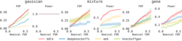
Figure 1: ddlk controls fdr at the nominal rate and achieves highest power on a variety of benchmarks. For each benchmark, we show the fdp and power of each knockoff method.

Each experiment involves three stages. First, we fit a knockoff generator using a dataset of covariates $\{{\bm{x}}^{(i)}\}_{i=1}^{N}$. Next, we fit a response model $\hat{q}_{\text{response}}({\mathbf{y}}\mid{\mathbf{x}};\gamma)$, and use its performance on a held-out set to create a knockoff statistic $w_{j}$ for each feature ${\mathbf{x}}_{j}$. We detail the construction of these test statistics in appendix E. Finally, we apply a knockoff filter to the statistics $\{w_{j}\}_{j=1}^{d}$ to select features at a nominal fdr level $p$, and measure the ability of each knockoff method to select relevant features while maintaining fdr at $p$. For the synthetic and semi-synthetic tasks, we repeat these three stages 30 times to obtain interval estimates of each performance metric.

In our experiments, we assume ${\mathbf{x}}$ to be real-valued with continuous support and decompose the models $\hat{q}_{\text{joint}}$ and $\hat{q}_{\text{knockoff}}$ via the chain rule: $q({\mathbf{x}}\mid\cdot)=q({\mathbf{x}}_{1}\mid\cdot)\prod_{j=2}^{d}q({\mathbf{x}}_{j}\mid\cdot,{\mathbf{x}}_{1},\dots,{\mathbf{x}}_{j-1}).$ For each conditional distribution, we fit a mixture density network [1] where the number of mixture components is a hyperparameter. In principle, any model that produces an explicit likelihood value can be used to model each conditional distribution.

Fitting $\hat{q}_{\text{joint}}$ involves using samples from a dataset, but fitting $\hat{q}_{\text{knockoff}}$ involves sampling from $\hat{q}_{\text{knockoff}}$. This is a potential issue because the gradient of the ddlk objective eq. 8 with respect to $\phi$ is difficult to compute as it involves integrating $\hat{q}_{\text{knockoff}}$, which depends on $\phi$. To solve this, we use an implicit reparameterization [5] of mixture densities. Further details of this formulation are presented in appendix B.

Across each benchmark involving ddlk, we vary only the $\lambda$ entropy regularization parameter based on the amount of dependence among covariates. The number of parameters, learning rate, and all other hyperparameters are kept constant. To sample swaps $H$, we sample using a straight-through Gumbel-Softmax estimator [9]. This allows us to sample binary values for each swap, but use gradients of a continuous approximation during optimization. For brevity, we present the exact hyperparameter details for ddlk in appendix C.

We run each experiment on a single CPU with 4GB of memory. Ddlk takes roughly 40 minutes in total to fit both $\hat{q}_{\text{joint}}$ and $\hat{q}_{\text{knockoff}}$ on a 100-dimensional dataset.

Synthetic benchmarks.

Our tests on synthetic data seek to highlight differences in power and fdr between each knockoff generation method. Each dataset in this section consists of $N=2000$ samples, 100 features, 20 of which are used to generate the response ${\mathbf{y}}$. We split the data into a training set ($70\%$) to fit each knockoff method, a validation set ($15\%$) used to tune the hyperparameters of each method, and a test set ($15\%$) for evaluating knockoff statistics.

[gaussian]: We first replicate the multivariate normal benchmark of Romano et al. [20]. We sample ${\mathbf{x}}\sim\mathcal{N}(0,\Sigma)$, where $\Sigma$ is a $d$-dimensional covariance matrix whose entries $\Sigma_{i,j}=\rho^{|i-j|}$. This autoregressive Gaussian data exhibits strong correlations between adjacent features, and lower correlations between features that are further apart. We generate ${\mathbf{y}}\mid{\mathbf{x}}\sim\mathcal{N}(\langle{\mathbf{x}},\alpha\rangle,1)$, where coefficients for the important features are drawn as $\alpha_{j}\sim\frac{100}{\sqrt{N}}\cdot\text{Rademacher}(0.5)$. In our experiments, we set $\rho=0.6$. We let the ddlk entropy regularization parameter $\lambda=0.1$. Our model $\hat{q}_{\text{response}}$ for ${\mathbf{y}}\mid{\mathbf{x}}$ is a $1$-layer neural network with $200$ parameters.

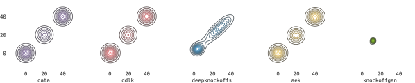
Figure 2: Ddlk closely models the modes, covariances, and mixture proportions of the mixture dataset. Auto-Encoding Knockoffs also capture every mode, but does so by overfitting to the covariates. Deep Knockoffs are able to match the first two moments, but fail to capture every mode. KnockoffGAN suffers from mode collapse and fails to capture every mode.

[mixture]: To compare each method on its ability to generate non-Gaussian knockoffs, we use a mixture of autoregressive Gaussians. This is a more challenging benchmark as each covariate is multi-modal, and highly correlated with others. We sample ${\mathbf{x}}\sim\sum_{k=1}^{K}\pi_{k}\mathcal{N}(\mu_{k},\Sigma_{k})$, where each $\Sigma_{k}$ is a $d$-dimensional covariance matrix whose $(i,j)$th entry is $\rho_{k}^{|i-j|}$. We generate ${\mathbf{y}}\mid{\mathbf{x}}\sim\mathcal{N}(\langle{\mathbf{x}},\alpha\rangle,1)$, where coefficients for the important features are drawn as $\alpha_{j}\sim\frac{100}{\sqrt{N}}\cdot\text{Rademacher}(0.5)$. In our experiments, we set $K=3$, and $(\rho_{1},\rho_{2},\rho_{3})=(0.6,0.4,0.2)$. Cluster centers are set to $(\mu_{1},\mu_{2},\mu_{3})=(0,20,40)$, and mixture proportions are set to $(\pi_{1},\pi_{2},\pi_{3})=(0.4,0.2,0.4)$. We let the ddlk entropy regularization parameter $\lambda=0.001$. Figure 2 visualizes two randomly selected dimensions of this data.

Results.

Figure 1 compares the average fdp and power (percentage of important features selected) of each knockoff generating method. The average fdp is an empirical estimate of the fdr. In the case of the gaussian dataset, all methods control fdr at or below the the nominal level, while achieving 100% power to select important features. The main difference between each method is in the calibration of null statistics. Recall that a knockoff filter assumes a null statistic to be positive or negative with equal probability, and features with negative statistics below a threshold are used to control the number of false discoveries when features with positive statistics above the same threshold are selected. Ddlk produces the most well calibrated null statistics as evidenced by the closeness of its fdp curve to the dotted diagonal line.

Figure 1 also demonstrates the effectiveness of ddlk in modeling non-Gaussian covariates. In the case of the mixture dataset, ddlk achieves significantly higher power than the baseline methods, while controlling the fdr at nominal levels. To understand why this may be the case, we plot the joint distribution of two randomly selected features in fig. 2. Ddlk and Auto-Encoding Knockoffs both seem to capture all three modes in the data. However, Auto-Encoding Knockoffs tend to produce knockoffs that are very similar to the original features, and yield lower power when selecting variables, shown in fig. 1. Deep Knockoffs manage to capture the first two moments of the data – likely due to an explicit second-order term in the objective function – but tend to over-smooth and fail to properly estimate the knockoff distribution. KnockoffGAN suffers from mode collapse, and fails to capture even the first two moments of the data. This yields knockoffs that not only have low power, but also fail to control fdr at nominal levels.

Robustness of ddlk to entropy regularization.

To provide guidance on how to set the entropy regularization parameter, we explore the effect of $\lambda$ on both fdr control and power. Intuitively, lower values of $\lambda$ will yield solutions of $\hat{q}_{\text{knockoff}}$ that may satisfy eq. 1 and control fdr well, but may also memorize the covariates and yield low power. Higher values of $\lambda$ may help improve power, but at the cost of fdr control. In this experiment, we again use the gaussian dataset, but vary $\lambda$ and the correlation parameter $\rho$. Figure 3 highlights the performance of ddlk over various settings of $\lambda$ and $\rho$. We show a heatmap where each cell represents the RMSE between the nominal fdr and mean fdp curves over 30 simulations. In each of these settings ddlk achieves a power of 1, so we only visualize fdp. We observe that the fdp of ddlk is very close to its expected value for most settings where $\lambda\leq 0.1$. This is true over a wide range of $\rho$ explored, demonstrating that ddlk is not very sensitive to the choice of this hyperparameter. We also notice that data with weaker correlations see a smaller increase in fdp with larger values of $\lambda$. In general, checking the fdp on synthetic responses generated conditional on real covariates can aid in selecting $\lambda$.

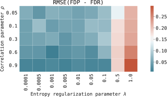
Figure 3: ddlk is robust to choices of entropy regularization parameter $\lambda$. For most choices of $\lambda\leq 0.1$, ddlk achieves fdp very close to that of the nominal fdr rate. This figure shows the RMSE between the expected and actual fdp curves.

Semi-synthetic benchmark.

[gene]: In order to evaluate the fdr and power of each knockoff method using covariates found in a genomics context, we create a semi-synthetic dataset. We use RNA expression data of 963 cancer cell lines from the Genomics of Drug Sensitivity in Cancer study [24]. Each cell line has expression levels for 20K genes, of which we sample 100 such that every feature is highly correlated with at least one other feature. We create 30 independent replications of this experiment by repeating the following process. We first sample a gene ${\mathbf{x}}_{1}$ uniformly at random, adding it to the set $\mathcal{X}$. For ${\mathbf{x}}_{j}$, $j>1$, we sample ${\mathbf{x}}_{k}$ uniformly at random from $\mathcal{X}$ and compute the set of $50$ genes not in $\mathcal{X}$ with the highest correlation with ${\mathbf{x}}_{k}$. From this set of $50$, we uniformly sample a gene ${\mathbf{x}}_{j}$ and add it to the feature set. We repeat this process for $j=2,\ldots,100$, yielding $100$ genes in total.

We generate ${\mathbf{y}}\mid{\mathbf{x}}$ using a nonlinear response function adapted from a study on feature selection in neural network models of gene-drug interactions [14]. The response consists of a nonlinear term, a second-order term, and a linear term. For brevity, appendix F contains the full simulation details. We let ddlk entropy regularization parameter $\lambda=0.001$.

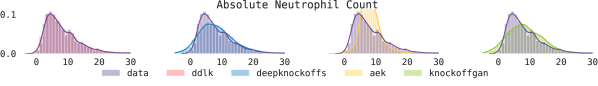
Figure 4: ddlk learns the marginals of COVID-19 data better than competing baselines. We plot the marginal distribution of a feature in a COVID-19 dataset, and the corresponding marginal of samples from each knockoff method.

Results.

Figure 1 (right) highlights the empirical fdp and power of each knockoff generating method in the context of gene. All methods control the fdr below the nominal level, but the average fdp of ddlk at fdr thresholds below 0.3 is closer to its expected value. This range of thresholds is especially important as nominal levels of fdr below 0.3 are most used in practice. In this range, ddlk achieves power on par with Deep Knockoffs at levels below 0.1, and higher power everywhere else. Auto-Encoding Knockoffs and KnockoffGAN achieve noticeably lower power across all thresholds. Deep Knockoffs perform well here likely due to a lack of strong third or higher moments of dependence between features. We attribute the success of ddlk and Deep Knockoffs to their ability to model highly correlated data.

COVID-19 adverse events.

[covid-19]: The widespread impact of COVID-19 has led to the deployment of machine learning models to guide triage. Data for COVID-19 is messy because of both the large volume of patients and the changing practice for patient care. Establishing trust in models for COVID-19 involves vetting the training data to ensure it does not contain artifacts that models can exploit. Conditional independence tests help achieve this goal in two ways: (a) they highlight which features are most important to the response, and (b) they prune the feature set for a deployed model, reducing the risk of overfitting to processes in a particular hospital. We apply each knockoff method to a large dataset from one of the epicenters of COVID-19 to understand the features most predictive of adverse events.

We use electronic health record data on COVID-positive patients from a large metropolitan health network. Our covariates include demographics, vitals, and lab test results from every complete blood count (cbc) taken for each patient. The response ${\mathbf{y}}\mid{\mathbf{x}}$ is a binary label indicating whether or not a patient had an adverse event (intubation, mortality, ICU transfer, hospice discharge, emergency department representation, O2 support in excess of nasal cannula at 6 L/min) within 96 hours of their cbc. There are 17K samples of 37 covariates in the training dataset, 5K in a validation set, and 6K in a held-out test set. We let the ddlk entropy regularization parameter $\lambda=0.1$. In this experiment, we use gradient boosted regression trees [6, 11] as our $\hat{q}_{\text{response}}({\mathbf{y}}\mid{\mathbf{x}};\gamma)$ model, and expected log-likelihood as a knockoff statistic. We also standardize the data in the case of Deep Knockoffs since mmds that use the radial basis function (rbf) kernel with a single bandwidth parameter work better when features are on the same scale.

Feature	DDLK	Deep Knockoffs	AEK	KnockoffGAN	Validated
Eosinophils count	✓	✗	✗	✗	✓
Eosinophils percent	✓	✓	✗	✗	✗
Blood urea nitrogen	✓	✗	✗	✗	✓
Ferritin	✓	✗	✗	✗	✗
O2 Saturation	✓	✗	✗	✗	✓
Heart rate	✓	✗	✗	✗	✓
Respiratory rate	✓	✓	✗	✗	✓
O2 Rate	✓	✓	✓	✓	✓
On room air	✓	✓	✓	✓	✓
High O2 support	✓	✓	✓	✓	✓
Age	✗	✗	✓	✓	✗

Table 1: Ddlk selects 10/37 features, 8 of which were found to be meaningful by doctors at a large metropolitan hospital. Here we show the union of covid-19 features selected by each knockoff method at a nominal fdr of 0.2. Deep Knockoffs, Auto-Encoding Knockoffs, and KnockoffGAN exhibit lower power to select important features.

Results.

As COVID-19 is a recently identified disease, there is no ground truth set of important features for this dataset. We therefore use each knockoff method to help discover a set of features at a nominal fdr threshold of $0.2$, and validate each feature by manual review with doctors at a large metropolitan hospital. Table 1 shows a list of features returned by each knockoff method, and indicates whether or not a team of doctors thought the feature should have clinical relevance.

We note that ddlk achieves highest power to select features, identifying 10 features, compared to 5 by DeepKnockoffs, and 4 each by Auto-Encoding Knockoffs and KnockoffGAN. To understand why, we visualize the marginal distributions of each covariate in, and the respective marginal distribution of samples from each knockoff method, in fig. 4.

We notice two main differences between ddlk and the baselines. First, ddlk is able to fit asymmetric distributions better than the baselines. Second, despite the fact that the implementation of ddlk using mixture density networks is misspecified for discrete variables, ddlk is able to model them better than existing baselines. This implementation uses continuous models for ${\mathbf{x}}$, but is still able approximate discrete distributions well. The components of each mixture appear centered around a discrete value, and have very low variance as shown in fig. 5. This yields a close approximation to the true discrete marginal. We show the marginals of every feature for each knockoff method in appendix G.

5 Conclusion

Ddlk is a generative model for sampling knockoffs that directly minimizes a ${\mathrm{KL}}$ divergence implied by the knockoff swap property. The optimization for ddlk involves first maximizing the explicit likelihood of the covariates, then minimizing the ${\mathrm{KL}}$ divergence between the joint distribution of covariates and knockoffs and any swap between them. To ensure ddlk satisfies the swap property under any swap indices, we use the Gumbel-Softmax trick to learn swaps that maximize the ${\mathrm{KL}}$ divergence. To generate knockoffs that satisfy the swap property while maintaining high power to select variables, ddlk includes a regularization term that encourages high conditional entropy of the knockoffs given the covariates. We find ddlk to outperform various baselines on several synthetic and real benchmarks including a task involving a large dataset from one of the epicenters of COVID-19.

Broader Impact

There are several benefits to using flexible methods for identifying conditional independence like ddlk. Practitioners that care about transparency have traditionally eschewed deep learning, but methods like ddlk can present a solution. By performing conditional independence tests with deep networks and by providing guarantees on the false discovery rate, scientists and practitioners can develop more trust in their models. This can lead to greater adoption of flexible models in basic sciences, resulting in new discoveries and better outcomes for the beneficiaries of a deployed model. Conditional independence can also help detect bias from data, by checking if an outcome like length of stay in a hospital was related to a sensitive variable like race or insurance type, even when conditioning on many other factors.

While we believe greater transparency can only be better for society, we note that interpretation methods for machine learning may not exactly provide transparency. These methods visualize only a narrow part of a model’s behavior, and may lead to gaps in understanding. Relying solely on these domain-agnostic methods could yield unexpected behavior from the model. As users of machine learning, we must be wary of too quickly dismissing the knowledge of domain experts. No interpretation technique is suitable for all scenarios, and different notions of transparency may be desired in different domains.

Appendix

Appendix A Proofs

A.1 Proof of theorem 3.1

Let $\mu$ be a probability measure defined on a measurable space. Let $f_{H}$ be a swap function using indices $H\subseteq[d]$. If ${\bm{v}}$ is a sample from $\mu$, the probability law of $f_{H}({\bm{v}})$ is $\mu\circ f_{H}$.

Proof.

The swap operation $f_{H}$ on $[{\mathbf{x}},{\widetilde{\mathbf{x}}}]$ swaps coordinates in the following manner: for each $j\in H$, the $j$th and $(j+d)$th coordinates are swapped. Let $(E,\mathcal{E})$ be a measurable space, where elements of $E$ are $2d$-dimensional vectors, and $\mathcal{E}$ is a $\sigma$-algebra on $E$. Let $(F,\mathcal{F})$ also be a measurable space where each element of $F$ is an element of $E$ but with the $j$th coordinate swapped with the $(j+d)$th coordinate for each $j\in H$. Similarly, let $\mathcal{F}$ be constructed by applying the same swap transformations to each element of $\mathcal{E}$. $\mathcal{F}$ is a $\sigma$-algebra as swaps are one-to-one transformations, and $\mathcal{E}$ is a $\sigma$-algebra.

We first show that $f_{H}$ is a measurable function with respect to $\mathcal{E}$ and $\mathcal{F}$. This is true by construction of the measurable space $(F,\mathcal{F})$. For every element $B\in\mathcal{F}$, $f_{H}^{-1}(B)\in\mathcal{E}$.

We can now construct a mapping $\mu\circ f_{H}^{-1}(B)$ for all $B\in\mathcal{F}$. This is the pushforward measure of $\mu$ under transformation $f_{H}$, and is well defined because $f_{H}$ is measurable.

Using the fact that a swap applied twice is the identity, we get $f_{H}=f_{H}^{-1}$. With this, we see that the probability measure on $(F,\mathcal{F})$ is $\mu\circ f_{H}^{-1}=\mu\circ f_{H}$. ∎

A.2 Alternative derivation of theorem 3.1 for continuous random variables

In this section we derive theorem 3.1 for continuous random variables in an alternative manner. Let ${\mathbf{x}}$ be a set of covariates, and ${\widetilde{\mathbf{x}}}$ be a set of knockoffs. Let ${\mathbf{z}}=[{\mathbf{x}},{\widetilde{\mathbf{x}}}]$, and ${\mathbf{w}}=[{\mathbf{x}},{\widetilde{\mathbf{x}}}]_{\text{swap}(H)}$ where $H$ is a set of coordinates in which we swap ${\mathbf{x}}$ and ${\widetilde{\mathbf{x}}}$. Recall that a swap operation on ${\mathbf{z}}$ is an affine transformation ${\mathbf{w}}=\mathbf{A}{\mathbf{z}}$, where $\mathbf{A}$ is a permutation matrix. Using this property, we get:

$$q_{\mathbf{w}}({\mathbf{z}})=\left|\text{det}\left(\frac{\partial\mathbf{A}^{-1}{\mathbf{w}}}{\partial{\mathbf{w}}}\right)\right|\cdot q_{{\mathbf{z}}}(\mathbf{A}^{-1}{\mathbf{z}})=q_{{\mathbf{z}}}(\mathbf{A}^{-1}{\mathbf{z}})=q_{{\mathbf{z}}}(\mathbf{A}{\mathbf{z}})=q_{{\mathbf{z}}}({\mathbf{w}}).$$

The first step is achieved by using a change of variables, noting that $\mathbf{A}$ is invertible, and ${\mathbf{z}}=\mathbf{A}^{-1}{\mathbf{w}}$. The determinant of the Jacobian here is just the determinant of $\mathbf{A}^{-1}$. $\mathbf{A}^{-1}$ is a permutation matrix whose parity is even, meaning its determinant is $1$, and that $\mathbf{A}^{-1}=\mathbf{A}$. I.e. the density of the swapped variables evaluated at ${\mathbf{z}}$ is equal to the original density evaluated at ${\mathbf{w}}$.

A.3 Proof of lemma 3.2

Recall lemma 3.2:

Worst case swaps: Let $q(H;\beta)$ be the worst case swap distribution. That is, the distribution over swap indices that maximizes

$$\mathbb{E}_{H\sim q(H;\beta)}\text{KL}(\hat{q}_{\text{joint}}({\mathbf{x}};\theta)\hat{q}_{\text{knockoff}}({\widetilde{\mathbf{x}}}\mid{\mathbf{x}};\phi)\parallel\hat{q}_{\text{joint}}({\mathbf{u}};\theta)\hat{q}_{\text{knockoff}}({\widetilde{\mathbf{u}}}\mid{\mathbf{u}};\phi))$$

with respect to $\beta$. If this quantity is minimized with respect to $\phi$, knockoffs sampled from $\hat{q}_{\text{knockoff}}$ will satisfy the swap property in eq. 1 for any swap $H$ in the power set of $[d]$.

Proof.

If

$$\mathbb{E}_{H\sim q(H;\beta)}\text{KL}(\hat{q}_{\text{joint}}({\mathbf{x}};\theta)\hat{q}_{\text{knockoff}}({\widetilde{\mathbf{x}}}\mid{\mathbf{x}};\phi)\parallel\hat{q}_{\text{joint}}({\mathbf{u}};\theta)\hat{q}_{\text{knockoff}}({\widetilde{\mathbf{u}}}\mid{\mathbf{u}};\phi))$$ (9)

is minimized with respect to $\phi$ but maximized with respect to $\beta$, then for any other distribution $q(H;\beta^{\prime})$, eq. 9 will be lesser. Minimizing eq. 9, which is non-negative, with respect to $\phi$ implies that for any swap $H$ sampled from $q(H;\beta)$ and for any knockoff ${\widetilde{\mathbf{x}}}$ sampled from $\hat{q}_{\text{knockoff}}$,

$$[{\mathbf{x}},{\widetilde{\mathbf{x}}}]\overset{d}{=}[{\mathbf{x}},{\widetilde{\mathbf{x}}}]_{\text{swap}(H)}.$$

As eq. 9 is also maximized with respect to $\beta$, swaps $H^{\prime}$ drawn from all other distributions $q(H^{\prime};\beta^{\prime})$ will only result in lower values of eq. 9. Therefore, the joint distribution $[{\mathbf{x}},{\widetilde{\mathbf{x}}}]$ will be invariant under any swap $H^{\prime}$ in the power set of $[d]$. ∎

A.4 Sufficient sets for swap condition expectation

Recall the swap property required of knockoffs highlighted in eq. 1:

$$[{\mathbf{x}},{\widetilde{\mathbf{x}}}] \overset{d}{=}[{\mathbf{x}},{\widetilde{\mathbf{x}}}]_{\text{swap}(H)}$$

where $H\subseteq[d]$ is a set of coordinates under which we swap the covariates and knockoffs. For valid knockoffs, this equality in distribution must hold for any such $H$. One approach to check if knockoffs are valid is to verify this equality in distribution for all singleton sets $\{j\}\subset[d]$ [20, 10]. To check if the swap property eq. 1 holds under any $H=\{j_{1},\dots,j_{k}\}$, it suffices to check if eq. 1 holds under each of $\{j_{1}\},\dots,\{j_{k}\}$.

We can generalize this approach to check the validity of knockoffs under other collections of indices besides singleton sets using the following property. Let $H_{1},H_{2}\subseteq[d]$ and

$$[{\mathbf{x}},{\widetilde{\mathbf{x}}}] \overset{d}{=}[{\mathbf{x}},{\widetilde{\mathbf{x}}}]_{\text{swap}(H_{1})}$$

$$[{\mathbf{x}},{\widetilde{\mathbf{x}}}] \overset{d}{=}[{\mathbf{x}},{\widetilde{\mathbf{x}}}]_{\text{swap}(H_{2})}.$$

Then,

$$[{\mathbf{x}},{\widetilde{\mathbf{x}}}]_{\text{swap}(H_{1}\Delta H_{2})}\overset{d}{=}\left[[{\mathbf{x}},{\widetilde{\mathbf{x}}}]_{\text{swap}(H_{1})}\right]_{\text{swap}(H_{2})}\overset{d}{=}\left[{\mathbf{x}},{\widetilde{\mathbf{x}}}\right]_{\text{swap}(H_{2})}\overset{d}{=}[{\mathbf{x}},{\widetilde{\mathbf{x}}}]$$

where $H_{1}\Delta H_{2}$ is the symmetric difference of $H_{1}$ and $H_{2}$. Swapping the indices in $H_{1}\Delta H_{2}$ is equivalent to swapping the indices in $H_{1}$, then the indices in $H_{2}$. If $\exists j\in H_{1}\wedge j\in H_{2}$, swapping $j$ twice will negate the effect of the swap.

We can extend this property to $K$ sets and define sufficient conditions to check if the swap property holds. Let $\{A_{k}\}_{k=1}^{K}$ be a sequence of sets where each $A_{k}\subseteq[d]$. Let

$$A_{1}^{*} =A_{1}$$

$$\forall k\in[K],A_{k}^{*} =A_{k}\Delta A_{k-1}^{*}$$

$$A_{K}^{*} =\{j\}.$$

Checking the swap property eq. 1 under a sequence of swaps $\{A_{k}\}_{k=1}^{K}$ is equivalent to checking eq. 1 under the singleton set $\{j\}$. Therefore, the swap property must also hold under the singleton set $\{j\}$.

If collection of sets of swap indices $A$ contains a sub-sequence $\{A_{k}\}_{k=1}^{K}$ such that their sequential symmetric difference is the singleton $\{j\}$ for each $j\in[d]$, then a set of knockoffs that satisfies the swap property under each $A_{k}\in A$, will also satisfy the swap property under each singleton set, which is sufficient to generate valid knockoffs.

Appendix B Implicit reparameterization of mixture density networks

In our experiments, we decompose both $\hat{q}_{\text{joint}}$ and $\hat{q}_{\text{knockoff}}$ via the chain rule:

$$q({\mathbf{x}}\mid\cdot)=q({\mathbf{x}}_{1}\mid\cdot)\prod_{j=2}^{d}q({\mathbf{x}}_{j}\mid\cdot,{\mathbf{x}}_{1},\cdots,{\mathbf{x}}_{j-1}).$$

We model each conditional $q({\mathbf{x}}_{j}\mid\cdot)$ using mixture density networks [1] which take the form

$$q({\mathbf{x}}_{j}\mid\cdot)=\sum_{k=1}^{K}\pi_{k}(\cdot;\psi_{k})\mathcal{N}(\mu_{k}(\cdot;\eta_{k}),\sigma_{k}^{2}(\cdot;\omega_{k}))$$

where functions $\{\pi_{k}\}_{k=1}^{K}$, $\{\mu_{k}\}_{k=1}^{K}$, and $\{\sigma_{k}\}_{k=1}^{K}$ characterize a univariate gaussian mixture. These parameters of these functions are $[\psi_{1},\dots,\psi_{K},\nu_{1},\dots,\nu_{K},\omega_{1},\dots,\omega_{K}]$.

Fitting $\hat{q}_{\text{joint}}$.

Let $\theta$, the parameters of $\hat{q}_{\text{joint}}$ contain parameters for every conditional $q({\mathbf{x}}_{j}\mid{\mathbf{x}}_{1},\dots,{\mathbf{x}}_{j-1})$. The optimization of $\theta$ is straightforward:

$$\theta=\operatorname*{arg\,max}_{\theta}\mathcal{L}(\theta)=\operatorname*{arg\,max}_{\theta}\frac{1}{N}\sum_{i=1}^{N}\log\hat{q}_{\text{joint}}({\bm{x}}^{(i)};\theta)$$

only requires taking the derivative of $\mathcal{L}(\theta)$.

Fitting $\hat{q}_{\text{knockoff}}$.

Let $\phi$, the parameters of $\hat{q}_{\text{knockoff}}$ contain parameters for every conditional $q({\widetilde{\mathbf{x}}}_{j}\mid{\mathbf{x}}_{1},\dots,{\mathbf{x}}_{d},{\widetilde{\mathbf{x}}}_{1},\dots,{\widetilde{\mathbf{x}}}_{j-1})$. Recall the loss function $\mathcal{L}(\phi,\beta)$

$$\mathcal{L}(\phi,\beta)=\mathbb{E}_{H\sim\hat{q}_{\text{gumbel}}(\beta)}\mathbb{E}_{{\bm{x}}\sim\mathcal{D}_{N}}\mathbb{E}_{\widetilde{{\bm{x}}}\sim\hat{q}_{\text{knockoff}}({\widetilde{\mathbf{x}}}\mid{\bm{x}};\phi)}\log\frac{\hat{q}_{\text{joint}}({\bm{x}};\theta)\hat{q}_{\text{knockoff}}(\widetilde{{\bm{x}}}\mid{\bm{x}};\phi)^{1+\lambda}}{\hat{q}_{\text{joint}}({\bm{u}};\theta)\hat{q}_{\text{knockoff}}(\widetilde{{\bm{u}}}\mid{\bm{u}};\phi)}.$$

The optimization of $\phi$ requires $\nabla_{\phi}\mathcal{L}(\phi,\beta)$, which involves the derivative of an expectation with respect to to $\hat{q}_{\text{knockoff}}({\widetilde{\mathbf{x}}}\mid{\mathbf{x}};\phi)$. We use implicit reparameterization [5]. The advantage of implicit reparameterization over explicit reparameterization [13] is that an inverse standardization function $S_{\phi}^{-1}$ – which transforms random noise into samples from a distribution parameterized by $\phi$ – is not needed. Using implicit reparameterization, gradients of some objective $\mathbb{E}_{q({\mathbf{z}};\phi)}[f({\mathbf{z}})]$ can be rewritten as

$$\mathbb{E}_{q({\mathbf{z}};\phi)}[\nabla_{\phi}f({\mathbf{z}})] =\mathbb{E}_{q({\mathbf{z}};\phi)}[\nabla_{\mathbf{z}}f({\mathbf{z}})\nabla_{\phi}{\mathbf{z}}]$$

$$=\mathbb{E}_{q({\mathbf{z}};\phi)}[-\nabla_{\mathbf{z}}f({\mathbf{z}})(\nabla_{\mathbf{z}}S_{\phi}({\mathbf{z}}))^{-1}\nabla_{\phi}S_{\phi}({\mathbf{z}})].$$

We use this useful property to reparameterize gaussian mixture models. Let $q({\mathbf{z}};\phi)$ be a gaussian mixture model:

$$q({\mathbf{z}};\phi)=\sum_{k=1}^{K}\pi_{k}\mathcal{N}({\mathbf{z}};\mu_{k},\sigma_{k}^{2})$$

where $\phi=[\pi_{1},\dots,\pi_{K},\mu_{1},\dots,\mu_{K},\sigma_{1},\dots,\sigma_{K}]$. Let the standardization function $S_{\phi}$ be the CDF of $q({\mathbf{z}};\phi)$:

$$S_{\phi}({\mathbf{z}})=\sum_{k=1}^{K}\pi_{k}\Phi\left(\frac{{\mathbf{z}}-\mu_{k}}{\sigma_{k}}\right)$$

where $\Phi$ is the standard normal gaussian CDF. We use this to compute the gradient of ${\mathbf{z}}$ with respect to each parameter:

$$\nabla_{\pi_{k}}{\mathbf{z}} =-\frac{\Phi(\frac{{\mathbf{z}}-\mu_{k}}{\sigma_{k}})}{q({\mathbf{z}};\phi)}$$

$$\nabla_{\mu_{k}}{\mathbf{z}} =\frac{\pi_{k}\cdot\mathcal{N}({\mathbf{z}};\mu_{k},\sigma_{k}^{2})}{q({\mathbf{z}};\phi)}$$

$$\nabla_{\sigma_{k}}{\mathbf{z}} =\frac{\pi_{k}\cdot\left(\frac{{\mathbf{z}}-\mu_{k}}{\sigma_{k}}\right)\cdot\mathcal{N}({\mathbf{z}};\mu_{k},\sigma_{k}^{2})}{q({\mathbf{z}};\phi)}.$$

Putting it all together, we use the implicit reparameterization trick to implement each conditional distribution in $\hat{q}_{\text{joint}}$ and $\hat{q}_{\text{knockoff}}$.

Appendix C Implementation details and hyperparameter settings for ddlk experiments

We decompose $\hat{q}_{\text{joint}}$ and $\hat{q}_{\text{knockoff}}$ into the product of univariate conditional distributions using the product rule. We use mixture density networks [1] to parameterize each conditional distribution. Each mixture density network is a 3-layer neural network with 50 parameters in each layer and a residual skip connection from the input to the last layer. Each network outputs the parameters for a univariate gaussian mixture with 5 components. We initialize the network such that the modes are evenly spaced within the support of training data.

Using $\hat{q}_{\text{gumbel}}$, we sample binary swap matrices of the same dimension as the data. As we require discrete samples from the Gumbel-Softmax distribution, we implement a straight-through estimator [9]. The straight-through estimator facilitates sampling discrete indices, but uses a continuous approximation during backpropagation.

The $\hat{q}_{\text{joint}}$ model is optimized using Adam [12], with a learning rate of $5\times 10^{-4}$ for a maximum of 50 epochs. The $\hat{q}_{\text{knockoff}}$ model is optimized using Adam, with a learning rate of $1\times 10^{-3}$ for $\phi$ and $1\times 10^{-2}$ for $\beta$ for a maximum of 250 epochs. We also implement early stopping using validation loss using the PyTorch Lightning framework [4].

Our code can be found online by installing:

pip install -i https://test.pypi.org/simple/ ddlk==0.2

Compute resources.

We run each experiment on a single CPU core using 4GB of memory. Fitting $\hat{q}_{\text{joint}}$ for a 100-dimensional dataset with 2000 samples requires fitting 100 conditional models, and takes roughly 10 minutes. Fitting $\hat{q}_{\text{knockoff}}$ for the same data takes roughly 30 minutes.

Fitting ddlk to our covid-19 dataset takes roughly 15 minutes in total.

Appendix D Baseline model settings

For Deep Knockoffs and KnockoffGAN, we use code from each respective repository:

https://github.com/msesia/deepknockoffs

https://bitbucket.org/mvdschaar/mlforhealthlabpub/

and use the recommended hyperparameter settings.

At the time of writing this paper, there was no publicly available implementation for Auto-Encoding Knockoffs. We implemented Auto-Encoding Knockoffs with a vae with a gaussian posterior $q({\mathbf{z}}\mid{\mathbf{x}})\approx\mathcal{N}({\mathbf{z}};\mu_{\mathbf{z}}({\mathbf{x}}),\sigma_{\mathbf{z}}({\mathbf{x}}))$ and likelihood $p({\mathbf{x}}\mid{\mathbf{z}})\approx\mathcal{N}({\mathbf{x}};\mu_{\mathbf{x}}({\mathbf{z}}),\sigma_{\mathbf{x}}({\mathbf{z}}))$. Each of $\mu_{\mathbf{z}},\sigma_{\mathbf{z}},\mu_{\mathbf{x}}.\sigma_{\mathbf{x}}$ is a 2-layer neural network with 400 units in the first hidden layer, 500 units in the second, and ReLU activations. The outputs of networks $\sigma_{\mathbf{z}},\sigma_{\mathbf{x}}$ are exponentiated to ensure variances are non-negative. The outputs of network $\mu_{\mathbf{z}}$ and $\sigma_{\mathbf{z}}$ are of dimension $d_{\mathbf{z}}$, and the outputs of $\mu_{\mathbf{x}}$ and $\sigma_{\mathbf{x}}$ are of dimension $d$, the covariate dimension. For each dataset, we choose the dimension $d_{\mathbf{z}}$ of latent variable ${\mathbf{z}}$ that maximizes the estimate of the ELBO on a validation dataset. In our experiments, we search for $d_{\mathbf{z}}$ over the set $\{d_{\mathbf{z}}:10\leq d_{\mathbf{z}}\leq 200,d_{\mathbf{z}}\mod 10=0\}$. For each dataset, we use the following $d_{\mathbf{z}}$:

1. gaussian: 20

2. mixture: 140

3. gene: 30

4. covid-19: 60.

The neural networks are trained using Adam [12], with a learning rate of $1\times 10^{-4}$ for a maximum of 150 epochs. To avoid very large gradients, we standardize the data using the mean and standard deviation of the training set. To generate knockoffs ${\widetilde{\mathbf{x}}}$, we use the same approach prescribed by Liu and Zheng [15]. We first sample the latent variable ${\mathbf{z}}$ conditioned on the covariates using the posterior distribution:

$${\mathbf{z}}\sim\mathcal{N}\left({\mathbf{z}};\mu_{\mathbf{z}}({\mathbf{x}}),\sigma_{\mathbf{z}}({\mathbf{x}})\right).$$

This sample of ${\mathbf{z}}$ is then used to sample a knockoff ${\widetilde{\mathbf{x}}}$ using the likelihood distribution:

$${\widetilde{\mathbf{x}}}\sim\mathcal{N}\left({\mathbf{x}};\mu_{\mathbf{x}}({\mathbf{z}}),\sigma_{\mathbf{x}}({\mathbf{z}})\right).$$

Since these ${\widetilde{\mathbf{x}}}$ are standardized, we re-scale them by the the training mean and standard deviation.

Appendix E Robust model-based statistics for fdr-control

The goal of any knockoff method is to help compute test statistics for a conditional independence test. We employ a variant of holdout randomization tests (hrts) [23] to compute test statistics $w_{j}$ for each feature ${\mathbf{x}}_{j}$. We split dataset $\mathcal{D}_{N}:=\{({\bm{x}}^{(i)},{\bm{y}}^{(i)})\}_{i=1}^{N}$ into train and test sets $\mathcal{D}_{N}^{\text{(tr)}}$, and $\mathcal{D}_{N}^{\text{(te)}}$ respectively, then sample knockoff datasets $\widetilde{\mathcal{D}}_{N}^{\text{(tr)}}$ and $\widetilde{\mathcal{D}}_{N}^{\text{(te)}}$ conditioned on each. Next, a model $\hat{q}_{\text{response}}$ is fit with $\mathcal{D}_{N}^{\text{(tr)}}$.

To compute knockoff statistics with $\hat{q}_{\text{response}}$, we use a measure of performance $\mathcal{W}(\hat{q}_{\text{response}},\mathcal{D}_{N}^{\text{(te)}})$ on the test set. For real-valued ${\mathbf{y}}$, $\mathcal{W}$ is the mean squared-error, and for categorical ${\mathbf{y}}$, $\mathcal{W}$ is expected log-probability of ${\mathbf{y}}\mid{\mathbf{x}}$. A knockoff statistic $w_{j}:=\mathcal{W}(\hat{q}_{\text{response}},\mathcal{D}_{N}^{\text{(te)}})-\mathcal{W}(\hat{q}_{\text{response}},\widetilde{\mathcal{D}}_{j,N}^{\text{(te)}})$ is recorded for each feature ${\mathbf{x}}_{j}$, where $\widetilde{\mathcal{D}}_{j,N}^{\text{(te)}}$ is $\mathcal{D}_{N}^{\text{(te)}}$ but with the $j$th feature swapped with $\widetilde{\mathcal{D}}_{N}^{\text{(te)}}$.

In practice, we use use flexible models like neural networks or boosted trees for $\hat{q}_{\text{response}}$. While the model-based statistic above will satisfy the properties detailed in section 2 and control fdr, its ability to do so is hindered by imperfect knockoffs. In such cases, we observe that knockoff statistics for null features are centered around some $\zeta>0$, violating a condition required for empirical fdr control. This happens because if the covariates and knockoffs are not equal in distribution, models trained on the covariates will fit the covariates better than the knockoffs and inflate the value of test statistic $w_{j}$. This can lead to an increase in the false discovery rate as conditionally independent features may be selected if their statistic is larger than the selection threshold. To combat this, we propose a mixture statistic that trades off power for fdr-control.

The mixture statistic involves fitting a $\hat{q}_{\text{response}}$ model for each feature ${\mathbf{x}}_{j}$ using an equal mixture of data in $\mathcal{D}_{N}^{\text{(tr)}}$ and $\widetilde{\mathcal{D}}_{j,N}^{\text{(tr)}}$, then computing $\mathcal{W}$ as above. Such a $\hat{q}_{\text{response}}$ achieves lower performance on $\mathcal{D}_{N}^{\text{(te)}}$, but higher performance on $\widetilde{\mathcal{D}}_{j,N}^{\text{(te)}}$, yielding values of $w_{j}$ with modes closer to $0$, enabling finite sample fdr control. However, this fdr-control comes at the cost of power as the method’s ability to identify conditionally dependent features is reduced.

Appendix F Nonlinear response for gene experiments

We simulate the response ${\mathbf{y}}\mid{\mathbf{x}}$ for the gene experiment using a nonlinear response function designed for genomics settings [14]. The response consists of two first-order terms, a second-order term, and an additional nonlinearity in the form of a $\tanh$:

$$k \in[m/4]$$

$$\varphi^{(1)}_{k},\varphi^{(2)}_{k} \sim\mathcal{N}(1,1)$$

$$\varphi^{(3)}_{k},\varphi^{(4)}_{k},\varphi^{(5)}_{k},\varphi^{(6)}_{k} \sim\mathcal{N}(2,1)$$

$${\mathbf{y}}\mid{\mathbf{x}} =\epsilon+\sum_{k=1}^{m/4}\varphi^{(1)}_{k}{\mathbf{x}}_{4k-3}+\varphi^{(3)}_{k}{\mathbf{x}}_{4k-2}+\varphi^{(4)}_{k}{\mathbf{x}}_{4k-3}{\mathbf{x}}_{4k-2}+\varphi^{(5)}_{k}\tanh(\varphi^{(2)}_{k}{\mathbf{x}}_{4k-1}+\varphi^{(6)}_{k}{\mathbf{x}}_{4k})$$

where $m$ is the number of important features. In our experiments, we set $m=20$. This means that the first $20$ features are important, while the remaining $80$ are unimportant.

Appendix G Generating knockoffs for COVID-19 data

In this section, we visualize the marginals of each feature in our covid-19 dataset, and the marginals of knockoffs sampled from each method. Figures 5, 6, 7 and 8 plot the marginals of samples from ddlk, KnockoffGAN, Deep Knockoffs, and Auto-Encoding Knockoffs respectively. These provide insight into why ddlk is able to select more features at the same nominal fdr threshold of 0.2. We first notice that knockoff samples from ddlk match the marginals of the data very well. Ddlk is the only method that models asymmetric distributions well.

Despite our experiment using mixture density networks to implement ddlk, discrete data is also modeled well. For example the values of O2_support_above_NC – a binary feature indicating whether a patient required oxygen support greater than nasal cannula – are also the modes of a mixture density learned by ddlk. Samples from Auto-Encoding Knockoffs, KnockoffGAN, and Deep Knockoffs tend to place mass spread across these values.

Figure 5: The marginal distributions of knockoff samples from ddlk look very similar to those from the data. Despite this implementation of ddlk using mixture density networks, the modes of each marginal line up with discrete values in the data.

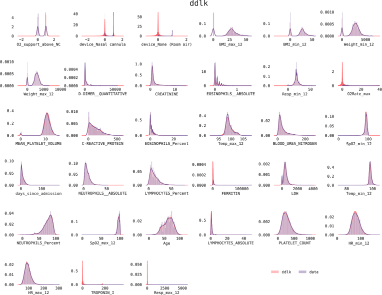
Figure 6: The marginals distributions of samples from KnockoffGAN match the data only when the feature ${\mathbf{x}}_{j}$ is univariate, and has roughly equal mass on either side of the mode.

Figure 7: The marginals distributions of samples from Deep Knockoffs match the data only when the feature ${\mathbf{x}}_{j}$ is univariate and has fat tails.

Figure 8: Auto-Encoding Knockoffs tend to learn underdispersed distributions for the covariates. Further, all of the marginal distributions learned are univariate and exhibit variance much smaller than that of the data.

References

- Bishop [1994] Christopher M Bishop. Mixture density networks. Technical report, Aston University, Birmingham, UK, 1994.
- Candes et al. [2016] E. Candes, Y. Fan, L. Janson, and J. Lv. Panning for Gold: Model-X Knockoffs for High-dimensional Controlled Variable Selection. ArXiv e-prints, October 2016.
- Candes et al. [2018] Emmanuel Candes, Yingying Fan, Lucas Janson, and Jinchi Lv. Panning for gold:‘model-x’knockoffs for high dimensional controlled variable selection. Journal of the Royal Statistical Society: Series B (Statistical Methodology), 80(3):551–577, 2018.
- Falcon [2019] WA Falcon. Pytorch lightning. GitHub. Note: https://github. com/williamFalcon/pytorch-lightning Cited by, 3, 2019.
- Figurnov et al. [2018] Mikhail Figurnov, Shakir Mohamed, and Andriy Mnih. Implicit reparameterization gradients. In Advances in Neural Information Processing Systems, pages 441–452, 2018.
- Friedman [2002] Jerome H Friedman. Stochastic gradient boosting. Computational statistics & data analysis, 38(4):367–378, 2002.
- Germain et al. [2015] Mathieu Germain, Karol Gregor, Iain Murray, and Hugo Larochelle. MADE: masked autoencoder for distribution estimation. CoRR, abs/1502.03509, 2015. URL http://arxiv.org/abs/1502.03509.
- Gulrajani et al. [2017] Ishaan Gulrajani, Faruk Ahmed, Martín Arjovsky, Vincent Dumoulin, and Aaron C. Courville. Improved training of wasserstein gans. CoRR, abs/1704.00028, 2017. URL http://arxiv.org/abs/1704.00028.
- Jang et al. [2016] Eric Jang, Shixiang Gu, and Ben Poole. Categorical reparameterization with gumbel-softmax. CoRR, abs/1611.01144, 2016. URL http://arxiv.org/abs/1611.01144.
- Jordon et al. [2019] James Jordon, Jinsung Yoon, and Mihaela van der Schaar. KnockoffGAN: Generating knockoffs for feature selection using generative adversarial networks. In International Conference on Learning Representations, 2019. URL https://openreview.net/forum?id=ByeZ5jC5YQ.
- Ke et al. [2017] Guolin Ke, Qi Meng, Thomas Finley, Taifeng Wang, Wei Chen, Weidong Ma, Qiwei Ye, and Tie-Yan Liu. Lightgbm: A highly efficient gradient boosting decision tree. In Advances in neural information processing systems, pages 3146–3154, 2017.
- Kingma and Ba [2014] Diederik P Kingma and Jimmy Ba. Adam: A method for stochastic optimization. arXiv preprint arXiv:1412.6980, 2014.
- Kingma et al. [2015] Durk P Kingma, Tim Salimans, and Max Welling. Variational dropout and the local reparameterization trick. In Advances in neural information processing systems, pages 2575–2583, 2015.
- Liang et al. [2018] Faming Liang, Qizhai Li, and Lei Zhou. Bayesian neural networks for selection of drug sensitive genes. Journal of the American Statistical Association, 113(523):955–972, 2018.
- Liu and Zheng [2018] Ying Liu and Cheng Zheng. Auto-encoding knockoff generator for fdr controlled variable selection. arXiv preprint arXiv:1809.10765, 2018.
- Maddison et al. [2016] Chris J. Maddison, Andriy Mnih, and Yee Whye Teh. The concrete distribution: A continuous relaxation of discrete random variables. CoRR, abs/1611.00712, 2016. URL http://arxiv.org/abs/1611.00712.
- Mescheder et al. [2017] Lars Mescheder, Sebastian Nowozin, and Andreas Geiger. The numerics of gans. In Advances in Neural Information Processing Systems, pages 1825–1835, 2017.
- Mescheder et al. [2018] Lars Mescheder, Andreas Geiger, and Sebastian Nowozin. Which training methods for gans do actually converge? arXiv preprint arXiv:1801.04406, 2018.
- Ramdas et al. [2015] Aaditya Ramdas, Sashank Jakkam Reddi, Barnabás Póczos, Aarti Singh, and Larry Wasserman. On the decreasing power of kernel and distance based nonparametric hypothesis tests in high dimensions. In Twenty-Ninth AAAI Conference on Artificial Intelligence, 2015.
- Romano et al. [2018] Yaniv Romano, Matteo Sesia, and Emmanuel J. Candès. Deep knockoffs, 2018.
- Salimans et al. [2016] Tim Salimans, Ian Goodfellow, Wojciech Zaremba, Vicki Cheung, Alec Radford, and Xi Chen. Improved techniques for training gans. In Advances in neural information processing systems, pages 2234–2242, 2016.
- Sesia et al. [2017] Matteo Sesia, Chiara Sabatti, and Emmanuel J Candès. Gene hunting with knockoffs for hidden markov models. arXiv preprint arXiv:1706.04677, 2017.
- Tansey et al. [2018] Wesley Tansey, Victor Veitch, Haoran Zhang, Raul Rabadan, and David M Blei. The holdout randomization test: Principled and easy black box feature selection. arXiv preprint arXiv:1811.00645, 2018.
- Yang et al. [2012] Wanjuan Yang, Jorge Soares, Patricia Greninger, Elena J Edelman, Howard Lightfoot, Simon Forbes, Nidhi Bindal, Dave Beare, James A Smith, I Richard Thompson, et al. Genomics of drug sensitivity in cancer (gdsc): a resource for therapeutic biomarker discovery in cancer cells. Nucleic acids research, 41(D1):D955–D961, 2012.