Ergodicity Bounds for the Markovian Queue With Time-Varying Transition Intensities, Batch Arrivals and One Queue Skipping Policy

Abstract. In this paper we revisit the Markovian queueing system with a single server, infinite capacity queue and one special queue skipping policy. Customers arrive in batches but are served one by one in any order. The size of the arriving batch becomes known upon its arrival and at any time instant the total number of customers in the system is also known. According to the adopted queue skipping policy if a batch, which size is greater than the current total number of customers in the system, arrives, all customers currently residing in the system are removed from it and the new batch is placed in the queue. Otherwise the new batch is lost and does not have effect on the system. The distribution of the total number of customers in the system is under consideration under assumption that the arrival intensity $\lambda(t)$ and/or the service intensity $\mu(t)$ are non-random functions of time. We provide the method for the computation of the upper bounds for the rate of convergence of system size to the limiting regime, whenever it exists, for any bounded $\lambda(t)$ and $\mu(t)$ (not necessarily periodic) and any distribution of the batch size. For periodic intensities $\lambda(t)$ and/or $\mu(t)$ and light-tailed distribution of the batch size it is shown how the obtained bounds can be used to numerically compute the limiting distribution of the queue size with the given error. Illustrating numerical examples are provided.

keywords: time-varying queueing system, queue skipping policy, rate of convergence bounds.

1 Introduction

The two most common viewpoints at a queueing system performance are the point of view of the system’s owner and of the system’s clients. Usually their goals are conflicting. While a client aims at minimizing one (or more) characteristic of the jobs, which he submits to the system (for example, job’s mean response time), the system’s owner seeks to maximize the utilization of the resources (for example, processor utilization). Both viewpoints have received attention from the operation research community in the last decades. But performance evaluation of queueing systems from the client’s perspective seems to have attracted more attention.

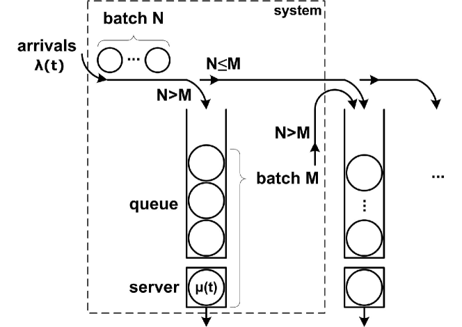
Figure 1: Model of the system with the queue skipping policy. It can be seen that the batches discarded from the system are (supposed not to be cleared but) offloaded to the next system with the same queue skipping policy and so on. This figure is the refinement of the figure 1 in [4].

If we limit ourselves only to single-server queues, then probably one of the best-known results here is the optimality of the SRPT (shortest remaining processing time) policy with respect to the job’s (or customer’s) mean response time. As is known, under the SRPT at all times the server is working on the “shortest” job. In [11] (based on the previous works [1, 13]) it was noticed that somewhat similar idea can be used to construct policies, which increase the utilization of all the servers in a system. One such policy, further referred to as the ”queue skipping” policy, works as follows (see Fig. 1). Assume that customers arrive to the system in batches, but are served one by one in any order. The size of the arriving batch becomes known upon its arrival and at any time the current system size (i.e. total number of customers in the system) is also known. According to the queue skipping policy if a batch, which size is greater than the current system size, arrives to the system, all current customers in the system are removed from it and the new batch is placed in the queue. Otherwise the new batch is lost and does not have affect on the system. In [11] the authors applied the time-reversed chains techniques (developed in [7, 8, 9, 10]), to study the performance of the $M/M/1$ system with such a queue skipping policy and generally distributed batch size, and, among other results, demonstrated the effect of the policy on the system utilization.

In this paper the effort is made to evaluate the performance of the same system, but with time-varying intensities i.e. when the arrival intensity $\lambda(t)$ and/or the service intensity $\mu(t)$ are non-random functions of time. Since the system is Markovian, the (time-varying) probability density function of the total number $X(t)$ of customers in the system evolves according to the system of ordinary differential equations (ODEs) – Kolmogorov forward equations. Except for very special cases, this system cannot be solved. Moreover if the batch size distribution has infinite support there are infinitely many ODEs in the system and the exact analytic solution is not possible. Here we adopt the approximation approach, which circumvents the difficulties by truncating the system of ODEs.

The contributions of this paper can be summarized as follows:

• We provide the method for the computation of the upper bounds for the rate of convergence of $X(t)$ to the limiting regime, whenever it exists, for any (not necessarily periodic) arrival intensity $\lambda(t)$ bounded from above by a constant, any locally integrable on $[0,\infty)$ service intensity $\mu(t)$, and any distribution of the batch size. This method uses the notion of the logarithmic norm of the linear operator and is based on the previous research [5, 19];

• For periodic intensities $\lambda(t)$ and/or $\mu(t)$ and light-tailed distribution of the batch size (which includes the geometric distribution and distributions with finite support) we show how one can compute the truncation threshold $t^{*}$, such that the probability distribution of $X(t)$ for $t>t^{*}$ “almost forgets” the distribution of $X(0)$. The latter means the all performance characteristics, which depend only on $X(t)$, can be considered as limiting characteristics for $t>t^{*}$ containing only a small error, which can be computed. Since under periodic intensities the solution of the system of ODEs governing the behaviour of $X(t)$ is also periodic, it is sufficient to compute numerically the solution only in the interval $[t^{*},t^{*}+T]$, where $T$ is chosen manually such that the interval $[t^{*},t^{*}+T]$ includes at least one period of the solution;

• Using the developed approximation approach, we numerically compare the utilization of the system with the queue skipping policy, periodic arrival intensity $\lambda(t)$, fixed service intensity $\mu$ and geometrically distributed batch size with mean $b$ with that of the classical $M_{t}/M/1/0$ queue with the same arrival intensity $\lambda(t)$ and service intensity $\mu/b$. This is intended to demonstrate the effect of the queue skipping policy on the system utilization.

Even though the obtained rate of convergence bounds do hold for any bounded arrival intensity $\lambda(t)$, locally integrable service intensity $\mu(t)$ and any distribution of the batch size, the proposed method for finding the truncation threshold $t^{*}$ has so far limited applicability. This is due to the fact that for long-tailed batch size distributions (i.e. those which have tails heavier than the geometric distribution) so far we were unable to find the condition, which guarantees the existence of the limiting regime of $X(t)$ (even for periodic intensities).

The paper is structured as follows. In Section 2 we repeat the description of the model. Section 3 contains the main result (see the Theorem and Corollaries 1–3). We demonstrate the method based on the logarithmic norm to bound (from above) the rate of convergence of $X(t)$ to the limiting regime (assuming that it exists). Here we also show that for geometrically distributed batch size the limiting regime always exists. In Section 4 the numerical example is given. Section 5 concludes the paper.

2 System description

Consider the $M_{t}/M_{t}/1$ queue with intensities being periodic functions of time and the queue skipping policy. Customers arrive to the system in batches according to the inhomogeneous Poisson process with intensity $\lambda(t)$. The size of an arriving batch becomes known upon its arrival and is the random variable with the given probability distribution $\{b_{n},n\geq 1\}$, having finite mean $\sum_{k=1}^{\infty}B_{k}$, $B_{k}=\sum_{n=k}^{\infty}b_{n}$. The adopted queue skipping policy implies that whenever a batch arrives to the system its size, say $\widehat{B}$, is compared with the current total number of customers in the system, say $\widetilde{B}$. If ${\widehat{B}}>{\widetilde{B}}$, then all customers, which are currently in the system, are instantly removed from it, and the whole batch ${\widehat{B}}$ is placed in the queue and the first customer in the batch enters server. If ${\widehat{B}}\leq{\widetilde{B}}$ the new batch leaves the system without having any effect on it. Whenever the server becomes free one customer from the queue (if there is any) enters server and gets served according to exponential distribution with intensity $\mu(t)$.

3 Main result

Let $X(t)$ be the total number of customers in the system at time $t$. From the system description it follows that $X(t)$ is the Markov chain with continuous time and discrete state space $\mathcal{X}=\{0,1,2,\dots,b^{*}\}$, where $b^{*}$ is the maximum possible batch size i.e. $b^{*}=\max_{n\geq 1}(b_{n}>0)$. If the batch size distribution has infinite support then the state space $\mathcal{X}$ is countable; otherwise it is finite.

Denote by $Q(t)$ the intensity matrix (infinitesimal generator) of $X(t)$. It is straightforward to see that $Q(t)$ has the form

$$Q(t)=\begin{pmatrix}-\lambda(t)&\lambda(t)b_{1}&\lambda(t)b_{2}&\dots\\ \mu(t)&-\left(\mu(t)+\lambda(t)B_{2}\right)&\lambda(t)b_{2}&\dots\\ 0&\mu(t)&-\left(\mu(t)+\lambda(t)B_{3}\right)&\dots\\ 0&0&\mu(t)&\dots\\ \vdots&\vdots&\vdots&\ddots\\ \end{pmatrix}.$$

We assume that $\lambda(t)$ and $\mu(t)$ are arbitrary non-random functions of $t$, locally integrable on $[0,\infty)$ and that the arrival intensity is bounded by a constant i.e. there exists $L>0$ such that $\lambda(t)\leq L<\infty$ for $t\geq 0$.

Denote by $p_{i}(t)=\mathbf{P}(X(t)=i)$ the probability that the Markov chain $X(t)$ is in state $i$ at time $t$. Let ${\mathbf{p}}(t)=(p_{0}(t),p_{1}(t),\dots)^{T}$ be the probability distribution vector at time $t$. Given any proper initial condition ${\mathbf{p}}(0)$, the probabilistic dynamics of the Markov chain $X\left(t\right)$ is described by the forward Kolmogorov system of differential equations

$$\frac{d}{dt}{\mathbf{p}}(t)=A(t){\mathbf{p}}(t),$$ (1)

where $A(t)=Q^{T}(t)$ is the transposed intensity matrix. Throughout the paper vectors are regarded as column vectors, ${\bf 0}$ denotes the vector consisting of zeros, $I$ denotes the identity matrix and $\cdot^{T}$ denotes the matrix transpose. The sizes of matrices will be clear from the context. The choice of vector norms will be the $l_{1}$-norm, that is, $\|{{\mathbf{p}}(t)}\|=\sum_{i\in\mathcal{X}}|p_{i}(t)|$; the operator norm will be the one induced by the $l_{1}$-norm on row vectors, that is, $\|A(t)\|=\sup_{j\in\mathcal{X}}\sum_{i\in\mathcal{X}}|a_{ij}(t)|$.

Recall that a Markov chain $X(t)$ is called weakly ergodic, if ${\|{\mathbf{p}}^{*}(t)-{\mathbf{p}}^{**}(t)\|\to 0}$ as $t\to\infty$ for any initial conditions ${\mathbf{p}}^{*}(0)$ and ${\mathbf{p}}^{**}(0)$, where ${\mathbf{p}}^{*}(t)$ and ${\mathbf{p}}^{**}(t)$ are the corresponding solutions of (1). The rate at which this difference tends to zero is called the rate of convergence. Below we present the method based on the logarithmic norm of a linear operator function, which allows one to bound from above this rate of convergence.

Using the normalization condition $p_{0}(t)=1-\sum_{i\geq 1,i\in\mathcal{X}}p_{i}(t)$ it can be checked that the system (1) can be rewritten as follows:

$$\frac{d}{dt}{{\mathbf{z}}}(t)=B(t){{\mathbf{z}}}(t)+{{\mathbf{f}}}(t),$$ (2)

where $B(t)=\left(b_{ij}(t)\right)_{i,j=1}^{\infty}$, $b_{ij}(t)=a_{ij}(t)-a_{i0}(t)$, and

$${{\mathbf{f}}}(t)=\left(\lambda(t)b_{1},\lambda(t)b_{2},\dots\right)^{T},$$

$${{\mathbf{z}}}(t)=\left(p_{1}(t),p_{2}(t),\dots\right)^{T},$$

$$B(t)={\footnotesize\left(\begin{array}[]{cccccccc}-\!\left(\mu(t)\!+\!\lambda(t)\right)&\mu(t)\!-\!\lambda(t)b_{1}&-\!\lambda(t)b_{1}&-\!\lambda(t)b_{1}&\cdots\\ 0&-\!\left(\mu(t)\!+\!\lambda(t)B_{2}\right)&\mu(t)\!-\!\lambda(t)b_{2}&-\!\lambda(t)b_{2}&\cdots\\ \vdots&\vdots&\vdots&\vdots&\ddots\\ \end{array}\right)\!.}$$

Note that the matrix $B(t)$ has no probabilistic meaning. Let ${{\mathbf{z}}}^{*}(t)$ and ${{\mathbf{z}}}^{**}(t)$ be the solutions of (2) corresponding to (different) initial conditions ${{\mathbf{z}}}^{*}(0)$ and ${{\mathbf{z}}}^{**}(0)$. Then for the vector ${{\mathbf{y}}}(t)={{\mathbf{z}}}^{*}(t)-{{\mathbf{z}}}^{**}(t)=\left({y}_{1}(t),{y}_{2}(t),\dots\right)^{T}$, which has coordinates of arbitrary signs, we have

$$\frac{d}{dt}{{\mathbf{y}}}(t)=B(t){{\mathbf{y}}}(t).$$ (3)

Thus all bounds on the rate of convergence to the limiting regime of $X(t)$ correspond to the same rate of convergence bounds of the solutions of the system (3). It is more convenient to study the rate of convergence using the transformed version $B^{*}(t)$ of $B(t)$ given by $B^{*}(t)=TB(t)T^{-1}$, where $T$ is the upper triangular matrix of the form

$$T=\left(\begin{array}[]{ccccccc}1&1&1&\cdots\\ 0&1&1&\cdots\\ 0&0&1&\cdots\\ \vdots&\vdots&\vdots&\ddots\\ \end{array}\right).$$

Let ${{\mathbf{u}}}(t)=T{{\mathbf{y}}}(t)=\left({u}_{1}(t),u_{2}(t),\dots\right)^{T}$. Then by multiplying (3) from the left by $T$ we obtain

$$\frac{d}{dt}{{\mathbf{u}}}(t)=B^{*}(t){{\mathbf{u}}}(t),$$ (4)

where ${{\mathbf{u}}}(t)$ is the vector with the coordinates of arbitrary signs and the matrix $B^{*}(t)$ has the following structure:

$$B^{*}(t)={\footnotesize\left(\begin{array}[]{ccccccc}-\!\mu(t)\!-\!\lambda(t)&\mu(t)&0&0&\cdots\\ 0&-\!\mu(t)\!-\!\lambda(t)B_{2}&\mu(t)&0&\cdots\\ 0&0&-\!\mu(t)\!-\!\lambda(t)B_{3}&\mu(t)&\cdots\\ \vdots&\vdots&\vdots&\vdots&\ddots\\ \end{array}\right)}.$$

The matrix $B^{*}(t)$ is essentially non-negative, i.e. all its off-diagonal elements are non-negative for any $t\geq 0$. From this fact it follows that, if the initial condition ${\mathbf{u}}(s)$ is non-negative, then any solution ${\mathbf{u}}(t)$ of (4) is non-negative for any $0\leq s\leq t$.

Now everything is ready to apply the method of logarithmic norm. Recall that the logarithmic norm $\gamma({B}(t))$ of the operator function $B(t)$ is defined as

$$\gamma({B}(t))=\lim_{h\to+0}h^{-1}\left(\|I+hB(t)\|-1\right).$$

Denote by $V(t,s)=V(t)V^{-1}(s)$ the Cauchy operator of the equation (3). Then $\|V(t,s)\|\leq e^{\,\int_{s}^{t}\gamma(B(u))\,du}$. For an operator function, which maps $l_{1}$-vectors into $l_{1}$-vectors and $B(t)$ is such an operator, $\gamma({B}(t))$ is expressed as:

$$\gamma({B}(t))=\sup_{j\in\mathcal{X}}\left(b_{jj}(t)+\sum_{i\in\mathcal{X},i\neq j}|b_{ij}(t)|\right).$$

If the matrix $B(t)$ is essentially non-negative then $\gamma({B}(t))=\sup_{j\in\mathcal{X}}\left(\sum_{i\in\mathcal{X}}b_{ij}(t)\right)$.

Let ${\{d_{i},\ i\geq 1\}}$ be a sequence of positive numbers such that $1=d_{1}\leq d_{2}\leq\dots$ and let $D=diag(d_{1},d_{2},\dots)$ be the diagonal matrix. By putting ${\bf w}(t)=D{\bf u}(t)$ in (4), we obtain the following equation

$$\frac{d}{dt}{\bf w}(t)=B^{**}(t){\bf w}(t),$$

where $B^{**}(t)=DB(t)^{*}D^{-1}=\left(b^{**}_{ij}(t)\right)_{i,j=1}^{\infty}$. Note that $B^{**}(t)$ is also nonnegative for any $t\geq 0$. Put

$$\alpha_{i}\left(t\right)=-\sum_{j=1}^{\infty}b_{ji}^{**}(t),\ i\geq 1,$$

and let $\alpha\left(t\right)=\inf_{i\geq 1}\alpha_{i}\left(t\right)$. We have that $\gamma({B^{**}}(t))=-\alpha\left(t\right)$ and

$$\|{\bf w}(t)\|\leq e^{-\int_{s}^{t}\alpha\left(u\right)\,du}\|{\bf w}(s)\|,$$

for any $s,t$ such that $0\leq s\leq t$.

Let $\delta<1$ be a positive number, and $d_{k+1}=\delta^{-k}$, $k\geq 1$. Then the values of $\alpha_{i}$ are equal to:

$$\alpha_{1}\left(t\right)=\lambda(t)+\mu(t),$$

$$\alpha_{k}\left(t\right)=\lambda(t)B_{k}+\mu(t)\left(1-\delta\right),\quad k\geq 2,$$

and therefore, we can bound $\alpha\left(t\right)$ by the following way:

$$\alpha\left(t\right)\geq\alpha^{*}\left(t\right)=\left(1-\delta\right)\mu(t).$$ (5)

So far we have assumed that the limiting regime of $X(t)$ exists. Its existence in the considered queue depends on the form of the batch size distribution $\{b_{n},n\geq 1\}$. Below we show that when the tail of the distribution is geometric or lighter then the limiting regime of $X(t)$ always exists, whereas for heavier tails the question remains open. We start with the analysis of (2). Let $V(t,s)$ be the Cauchy operator for (2). Then

$${\mathbf{z}}(t)=V(t){\mathbf{z}}(0)+\int_{0}^{t}{V}(t,\tau){\mathbf{f}}(\tau)\,d\tau.$$

Put ${\bf r}(t)=DT{\mathbf{z}}(t)$. Then instead of (2) we get:

$$\frac{d}{dt}{\bf r}(t)=B^{**}(t){\bf r}(t)+{\bf f^{**}}(t),$$ (6)

where ${\bf f^{**}}(t)=DT{\bf f}(t)$, and

$${\bf r}(t)=V^{**}(t){\bf r}(0)+\int_{0}^{t}{V}^{**}(t,\tau){\bf f^{**}}(\tau)\,d\tau,$$ (7)

where $\|V^{**}(t,s)\|\leq e^{-\int_{s}^{t}\alpha^{*}\left(u\right)\,du}$ due to (5). If there exist $N>0$ and $a>0$ such that

$$e^{-\int_{s}^{t}\alpha^{*}\left(u\right)\,du}\leq Ne^{-a(t-s)},$$ (8)

for any $0\leq s\leq t$, then we have exponential weak ergodicity in the corresponding norm.

Let there exist $0<q<1$ and $C>0$ such that $b_{k}\leq Cq^{k}$ for all $k\geq 1$. Then

$$\|{\bf r}(t)\|\leq\|V^{**}(t)\|\|{\bf r}(0)\|+$$

$$+\int_{0}^{t}\|{V}^{**}(t,\tau)\|\|{\bf f^{**}}(\tau)\|\,d\tau\leq Ne^{-at}\|{\bf r}(0)\|+$$

$$+\int_{0}^{t}Ne^{-a(t-\tau)}K\,d\tau\leq\frac{NK}{a}+o(1),$$ (9)

where

$$\|{\bf f^{**}}(t)\|=\|DT{\bf f}(t)\|=$$

$$=C\lambda(t)\left(\frac{d_{1}q}{1-q}+\frac{d_{2}q^{2}}{1-q}+\dots\right)\leq$$

$$\leq CL\left(\frac{q}{1-q}+\frac{\delta^{-1}q^{2}}{1-q}+\frac{\delta^{-2}q^{3}}{1-q}+\dots\right)=$$

$$=\frac{CL\delta q}{(\delta-q)(1-q)}=K,$$ (10)

for $\delta>q$.

Assume now that $b_{k}\to 0$ more slowly, say $b_{k}\geq k^{-s}$ for some $s>1$. Firstly note that essential non-negativity of $B^{**}(t)$ implies non-negativity of the matrix ${V}^{**}(t,s)$ for any $0\leq s\leq t$. Now if ${\bf r}(s)\geq{\bf 0}$ then ${\bf r}(t)\geq{\bf 0}$ for any $t\geq s$. This follows from non-negativity of ${\bf f^{**}}(t)$ and ${V}^{**}(t,s)$ in (7).

Put ${\bf r}(0)\geq{\bf 0}$. Then $\|{\bf r}(t)\|=\sum_{k\in\mathcal{X}}r_{k}(t)$, for any $t\geq 0$. From (6) for any $t\geq 0$ and for any $0<\delta<1$ we obtain

$$\frac{d}{dt}{\|\bf r}(t)\|=\sum_{k\in\mathcal{X}}\frac{d}{dt}{r_{k}}(t)\geq\|{\bf f^{**}}(t)\|=$$

$$=\lambda(t)\left(\left(b_{1}+b_{2}+b_{3}+\dots\right)+\delta^{-1}\left(b_{2}+b_{3}+\dots\right)+\right.$$

$$\left.+\delta^{-2}\left(b_{3}+\dots\right)+\dots\right)\geq\lambda(t)\sum_{k\geq 1}\delta^{-k}k^{-s}=\infty.$$

Hence the corresponding equation (6) does not have a limiting solution in the corresponding norm. Thus weak ergodicity and the existence of limiting characteristics is guaranteed only if the tail of the batch size distribution is geometric or lighter. We summarize the findings in the following

Theorem. Assume that exist $0<q<1$ and $C>0$ such that $b_{k}\leq Cq^{k}$ for all $k\geq 1$, and that

$$\int_{0}^{\infty}\mu(t)\,dt=+\infty.$$ (11)

Then the Markov chain $X(t)$ is weakly ergodic and for any initial condition ${\bf w}(0)$ and any $t\geq 0$ the following upper bound holds:

$$\|{\bf w}\left(t\right)\|\leq e^{-\int_{0}^{t}{\left(1-\delta\right)\mu\left(u\right)\,du}}\|{\bf w}(0)\|,$$

for any $\delta\in(q,1)$. If (8) holds for some $N>0$ and $a>0$, then $X(t)$ is exponentially weakly ergodic.

Now we can obtain the bounds in more natural norms. Firstly note that $\|{\mathbf{p}}^{*}(t)-{\mathbf{p}}^{**}(t)\|\leq 2\|{\mathbf{z}}^{*}(t)-{\mathbf{z}}^{**}(t)\|\leq 4\|{\bf w}(t)\|$ and $\|{\mathbf{z}}(t)\|_{1E}\leq W^{-1}\|\bf w(t)\|$ (see [19]), where $l_{1E}=$
$\left\{z(t)=(p_{1}(t),p_{2}(t),\ldots)^{T}:\|z(t)\|_{1E}\equiv\sum_{n\in\mathcal{X}}n|p_{n}(t)|<\infty\right\}$ and $W=\inf_{k\geq 1}\frac{d_{k}}{k}>0$.

Corollary 1. Under the assumptions of the Theorem the Markov chain $X(t)$ has a limiting mean, say $\phi(t)$, and the following rate of convergence bounds hold:

$$\|{\mathbf{p}}^{*}(t)-{\mathbf{p}}^{**}(t)\|\leq 4e^{-\int_{0}^{t}{\left(1-\delta\right)\mu\left(u\right)\,du}}\|{\bf w}(0)\|,$$ (12)

$$|E(t,k)-\phi(t)|\leq\frac{4}{W}e^{-\int_{0}^{t}{\left(1-\delta\right)\mu\left(u\right)\,du}}\|{\bf w}(0)\|,$$ (13)

where $E(t,k)=\sum_{n\in\mathcal{X}}np_{n}(t)$ is the mean number of customers in the system at time $t$, given that initially there where $k$ customers in the system i.e. $p_{k}(0)=1$.

Corollary 2. Let $X(t)$ be a homogeneous Markov chain i.e. $\lambda(t)=\lambda$ and $\mu(t)=\mu$. Then $X(t)$ is strongly ergodic and for any initial condition ${\bf w}(0)$ and any $t\geq 0$ the following upper bounds hold:

$$\|{\bf w}\left(t\right)\|\leq e^{-{\left(1-\delta\right)\mu t}}\|{\bf w}(0)\|,$$

$$\|{\mathbf{p}}^{*}(t)-{\mathbf{p}}^{**}(t)\|\leq 4e^{-{\left(1-\delta\right)\mu t}}\|{\bf w}(0)\|,$$

$$|E(t,k)-\phi(t)|\leq\frac{4}{W}e^{-{\left(1-\delta\right)\mu t}}\|{\bf w}(0)\|.$$

Corollary 3. Let the arrival intensity $\lambda(t)$ and the service intensity $\mu(t)$ be $1-$periodic. Then the assumptions of Theorem are equivalent to the inequality $\int_{0}^{1}\mu(t)\,dt>0$. Moreover the limiting probability distribution of the Markov chain $X(t)$ is $1-$periodic and the limiting mean is $1-$periodic as well.

From the Theorem and Corollaries 1–3 it follows that that the bounds on the rate of convergence hold for common intensity functions. If the latter are periodic in time then the limiting probability characteristics of the $X(t)$ (whenever they exists) are also periodic.

4 Numerical example

In all the examples presented below it is assumed that the batch size distribution $\{b_{k},\ k\geq 1\}$ is geometric i.e. $b_{k}=(1-q)q^{k-1}$, $k\geq 1$, $0<q<1$. It is also assumed that the arrival and/or transition intensities are periodic functions. Given that $\{b_{k},\ k\geq 1\}$ is geometric, irrespective of the parameter of the geometric distribution, periodic intensities guarantee the existence of the (periodic) limiting distribution of $X(t)$.

When the intensities are periodic but the batch size has a general distribution we were unable so far to find even sufficient conditions of the existence of the limiting distribution of $X(t)$.

Below we consider two examples: one is devoted to the discussion of the convergence bounds obtained and in the other the properties of the queue skipping policy are illustrated.

4.1 Example 1

In this example it is demonstrated how exactly the upper bound on the rate of convergence of $X(t)$ can be computed. Let both the arrival and service intensities be periodic and equal to $\lambda(t)=1+\sin(2\pi t)$ and $\mu(t)=1+\cos(2\pi t)$. Let $q=\frac{2}{3}$, i.e. the batch size distribution be $b_{k}=\frac{2^{k-1}}{3^{k}}$, $k\geq 1$, i.e. the mean batch size $\sum_{k=1}^{\infty}kb_{k}$ is $3$. From (9) it follows that in order to compute the upper bound on the rate of convergence, one needs to choose firstly $\delta\in(q,1)$ and secondly $\|{\bf w}(0)\|$. Namely, on the one hand, for the better rate of convergence we should choose smallest possible $\delta$ , and on the other hand, for better bounding of $\|{\bf w}(0)\|$ we should choose as much $\delta$ as possible. Put $\delta=\frac{5}{6}$. Thus $\alpha^{*}(u)=\frac{1}{6}\mu(t)$ and from (8) it follows that

$$e^{-\int_{s}^{t}\alpha^{*}(u)\,du}=e^{-\frac{1}{6}\int_{s}^{t}(1+\cos(2\pi u))\,du}\leq 2e^{-\frac{1}{6}(t-s)},$$

hence in the right part of (8) we can put $a=\frac{1}{6}$ and $N=2$. Now let us consider the choice of $\|{\bf w}(0)\|$.

Consider (10). We have $L=2$ and $C=\frac{1}{3}$. Thus $K=\frac{20}{3}$ in (10) and from (9) it follows that $\limsup_{t\to\infty}\|{\bf r}(t)\|\leq 80$. Since ${\bf w}(t)=DT{\bf y}(t)$, the inequality (9) guarantees that the $l_{1}$-norm of the limiting distribution of $X(t)$ does not exceed 80 i.e. $\|{\bf w}(0)\|\leq 80$. Thus (12) gives

$$\|{\mathbf{p}}^{*}(t)-{\mathbf{p}}^{**}(t)\|\leq 160e^{-\frac{t}{6}}$$ (14)

for any initial conditions ${\mathbf{p}}^{*}(0)$ and ${\mathbf{p}}^{**}(0)$. For example, if $t=80=t^{*}$ then the right part of (14) does not exceed $10^{-3}$ i.e. starting from $t>t^{*}$ the system “forgets” its initial state and the probability distribution $X(t)$ for $t>t^{*}$ can be regarded as the limiting distribution of $X(t)$. The error (in $l_{1}$-norm), which is thus made is not greater than $10^{-3}$. Moreover, since the limiting distribution of $X(t)$ is periodic, we are allowed to solve the system of ODEs only in the interval $[0,t^{*}+1]$. The probability distribution of $X(t)$ in the interval $[t^{*},t^{*}+1]$ is the estimate (with error not greater than $10^{-3}$ in $l_{1}$-norm) of the limiting probability distribution of $X(t)$. It must be noticed that since $b_{k}>0$ for all $k$, the system of ODEs contains infinite number of equations. Thus in order to solve it numerically one has to truncate the system. We perform this truncation according to the method in [20].

The upper bound on the rate of convergence of the mean number of customers in the system $E(t,k)$ to its limiting value $\phi(t)$ is computed in the same manner. Firstly recall that $d_{k+1}=\delta^{-k}$ and since $\delta=\frac{5}{6}$ has been fixed above, then $d_{k+1}=\delta^{-k}=\left(\frac{6}{5}\right)^{k}$. Thus $W=\inf_{k\geq 1}\frac{d_{k}}{k}=\frac{3}{4}$. Now consider (13). Thus $\|{\bf w}(0)\|\leq 80$ and from (13) it follows that

$$|E(t,k)-\phi(t)|\leq\frac{640}{3}e^{-\frac{t}{6}}$$ (15)

for any initial condition $X(0)=k$, $k\geq 0$. Thus for $t>t^{*}$ the value of $E(t,k)$ can be regarded as the limiting value of the mean number of customers and contains the error (in $l_{1}$-norm) not greater than $10^{-3}$.

In Fig. 2 and Fig. 3 one can see the graphs of $p_{0}(t)$ and $E(t,0)$ in the interval $[0,t^{*}=80]$. The ODEs are solved with the initial condition $X(0)=0$ i.e. the system is initially empty. It can be seen that the obtained upper bounds (14) and (15) are not tight: the systems enters periodic limiting regime before $t^{*}$.

4.2 Example 2

This example is devoted to the illustration of the properties of the queue skipping policy in the case when the transition intensities are time-dependent (purely Markov case is studied in [11]). For simplicity we assume that only the arrival intensity $\lambda(t)$ depends on time and the service intensity is constant i.e. $\mu(t)=\mu$, $t\geq 0$. Since the limiting regime always exists when the batch size distribution is geometric, no restrictions (additional to those required by the Theorem) are imposed on the arrival intensity $\lambda(t)$.

In Fig. 4, 5 and 6 one can see how the limiting probabilities $p_{0}(t)$, $p_{1}(t)$, $p_{2}(t)$ and $p_{3}(t)$ behave depending on the service intensity $\mu$. It is assumed that $\lambda(t)=0.8+0.1\sin(2\pi t)$, $b_{k}=2^{-k}$, $k\geq 1$, i.e. the mean batch size is $2$. Due to the low amplitude in the arrival intensity $\lambda(t)$, the amplitude of the limiting probabilities is also low and is dependent on the service intensity.

As in many other queueing systems, the idle probability $p_{0}(t)$ is one of the key performance indicators. In Fig. 7 and 8 one can see the behaviour of limiting value of $p_{0}(t)$, when the service intensity is fixed ($\mu(t)=\mu=1$). From the figures it can be seen that, as expected, the idle limiting probability tends to $0$ when the batch size or the arrival intensity increases.

Finally it is also of interest to compare the limiting idle probability $p_{0}(t)$ of the considered system with the queue skipping policy with the limiting idle probability in the pure blocking system i.e. $M_{t}/M/1/0$ queue under the same arrival intensity $\lambda(t)$. Since the arriving batch has mean size $(1-q)^{-1}$ we have to change the service intensity in the blocking system to $\mu(1-q)$. In Fig. 9 and 10 one can see the graphs of $p_{0}(t)$ in these two systems given that $\lambda(t)=0.8+0.1\sin(2\pi t)$ and $\mu=1$.

We observe that even the time-inhomogeneous system with the queue skipping policy (just like the homogeneous one studied in [11]) gives a much better utilisation than the pure blocking time-inhomogeneous system, when the mean batch size is large (i.e. $q$ is close to 1) and the arrival intensity is high.

5 Conclusion

Even though we have limited the discussion only to the geometric batch size, from Section 3 it can be seen that the method based on the logarithmic norm of a limiting operator allows us to upper bound the rate of convergence for any batch size distribution. The only open problem, which persists, is to find the conditions, which guarantee the existence of the limiting regime for any batch size distribution. So far we have not been able to do it but we believe that it is only the matter of the proper analytic point of view. This hope is supported by the fact that in time-homogeneous case such conditions are known (see [11]).

Although it is not mentioned above, being able to compute (approximately) the limiting mean of $X(t)$ allows one to use the time-varying Little’s law to compute the average sojourn time in the system (before a customer leaves the queue either due to an arrival or due to service completion).

The obtained results also show that in order to obtain the bounds on the rate of convergence one does not need to know the exact values of $\lambda(t)$ and $\mu(t)$. Instead it is sufficient to know the values of the integrals of type (11) i.e. the time-average intensities $\overline{\lambda}=\frac{1}{t}\lim_{t\to\infty}\int_{0}^{t}\lambda(u)du$ and $\overline{\mu}=\frac{1}{t}\lim_{t\to\infty}\int_{0}^{t}\mu(u)du$ (and not the exact values of $\lambda(t)$ and $\mu(t)$). In case of 1-periodic intensities $\lambda(t)$ and $\mu(t)$ the values $\overline{\lambda}$ and $\overline{\mu}$ are exactly the average arrival and service intensity over one period.

Acknowledgement. This research was supported by Russian Science Foundation under grant 19-11-00020.

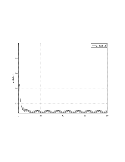
Figure 2: Rate of convergence of the empty system probability $p_{0}(t)$ in the interval $[0,80]$.

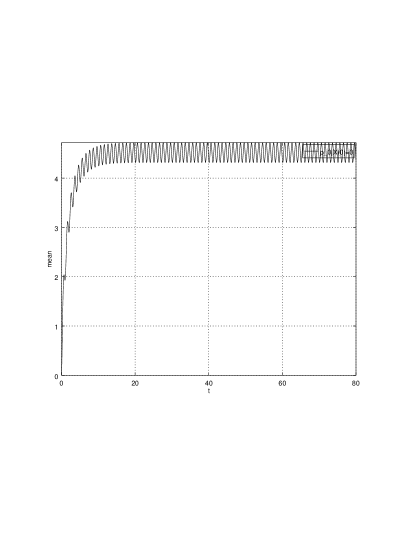
Figure 3: Rate of convergence of the mean number of customers $E(t,0)$ in the system in the interval $[0,80]$.

Figure 4: The limiting probabilities $p_{i}(t)$, $0\leq i\leq 3$, for $\mu=0.4$.

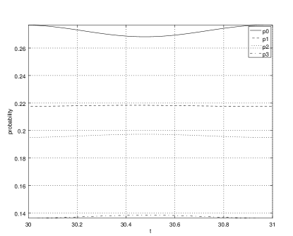
Figure 5: The limiting probabilities $p_{i}(t)$, $0\leq i\leq 3$, for $\mu=1$.

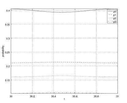
Figure 6: The limiting probabilities $p_{i}(t)$, $0\leq i\leq 3$, for $\mu=1.5$.

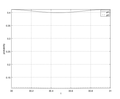
Figure 7: The limiting probability $p_{0}(t)$ for $q=0.7$ (dotted line) and for $q=0.3$ (solid line), $\lambda(t)=0.8+0.1\sin(2\pi t)$.

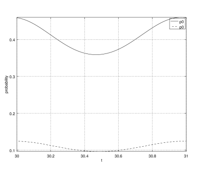
Figure 8: The limiting probability $p_{0}(t)$ for $q=0.7$ (dotted line) and for $q=0.3$ (solid line), $\lambda(t)=0.8+0.8\sin(2\pi t)$.

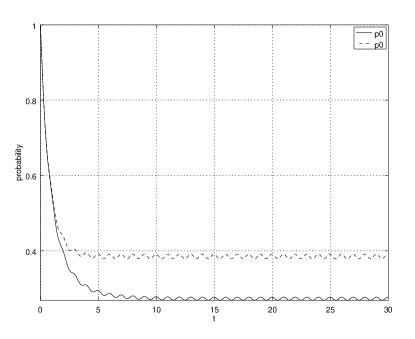
Figure 9: Rate of convergence of the empty system probability $p_{0}(t)$ for $q=0.5$, $\mu=1$ (solid line) and for $q=0$, $\mu=0.5$ (dotted line) in the interval $[0,30]$.

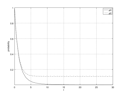
Figure 10: Rate of convergence of the empty system probability $p_{0}(t)$ for $q=0.9$, $\mu=1$ (solid line) and for $q=0$, $\mu=0.1$ (dotted line) in the interval $[0,30]$.

References

- [1] Balsamo, S., Harrison, P. G., Marin, A. (2010). A unifying approach to product-forms in networks with finite capacity constraints. ACM SIGMETRICS Performance Evaluation Review, 38(1), 25–36.
- [2] Burak, M. R., Korytkowski, P. (2020). Inhomogeneous CTMC Birth-and-Death Models Solved by Uniformization with Steady-State Detection. ACM Transactions on Modeling and Computer Simulation (TOMACS), 30(3), 1–S18.
- [3] Disney, R. L. (1962). Some multichannel queueing problems with ordered entry. Journal of Industrial Engineering, 13(1), 46–48.
- [4] Elsayed, E. A. (1983). Multichannel queueing systems with ordered entry and finite source. Computers & Operations Research, 10(3), 213–222.
- [5] Granovsky, B. L., Zeifman, A. (2004). Nonstationary queues: Estimation of the rate of convergence. Queueing Systems, 46(3-4), 363–388.
- [6] Grosof, I., Scully, Z., Harchol-Balter, M. (2018). SRPT for multiserver systems. Performance Evaluation, 127, 154–175.
- [7] Harrison, P. G. (2003). Turning back time in Markovian process algebra. Theor. Comput. Sci., 290(3), 1947–1986.
- [8] Harrison, P. G., Marin, A. (2014). Product-forms in multi-way synchronizations. The Computer Journal, 57(11), 1693–1710.
- [9] Kelly, F. P. (2011). Reversibility and stochastic networks. Cambridge University Press.
- [10] Marin, A., Balsamo, S., Fourneau, J. M. (2017). LB-networks: a model for dynamic load balancing in queueing networks. Performance Evaluation, 115, 38–53.
- [11] Marin, A., Rossi, S. (2020). A Queueing Model that Works Only on the Biggest Jobs. Lecture Notes in Computer Science book series (LNCS, volume 12039), 118–132.
- [12] Matsui, M. (2009). Manufacturing and service enterprise with risks. A Stochastic Management Approach. International Series in Operations Research & Management Science book series (ISOR, volume 125).
- [13] Pittel, B. (1979). Closed exponential networks of queues with saturation: the Jackson-type stationary distribution and its asymptotic analysis. Mathematics of Operations Research, 4(4), 357–378.
- [14] Razumchik, R., Zaryadov, I. (2016). Stationary blocking probability in multi-server finite queuing system with ordered entry and Poisson arrivals. Communications in Computer and Information Science book series (CCIS, volume 601), 344–357. Springer, Cham.
- [15] Schrage, L. (1968). A proof of the optimality of the shortest remaining processing time discipline. Operations Research, 16(3), 687–690.
- [16] Schwarz, J. A., Selinka, G., Stolletz, R. (2016). Performance analysis of time-dependent queueing systems: Survey and classification. Omega, 63, 170–189.
- [17] Whitt, W., You, W. (2019). Time-varying robust queueing. Operations Research, 67(6), 1766–1782.
- [18] Zeifman, A. I. (1989). Some properties of the loss system in the case of varying intensities. Autom. Remote Control, 1, 107–113.
- [19] Zeifman, A., Leorato, S., Orsingher, E., Satin, Y., Shilova, G. (2006). Some universal limits for nonhomogeneous birth and death processes. Queueing systems, 52(2), 139–151.
- [20] Zeifman, A. I., Korotysheva, A. V., Korolev, V. Y., Satin, Y. A. (2017). Truncation bounds for approximations of inhomogeneous continuous-time Markov chains. Theory of Probability & Its Applications, 61(3), 513–520.
- [21] Zeifman, A., Razumchik, R., Satin, Y., Kiseleva, K., Korotysheva, A., Korolev, V. (2018). Bounds on the rate of convergence for one class of inhomogeneous Markovian queueing models with possible batch arrivals and services. International Journal of Applied Mathematics and Computer Science, 28(1), 141–154.
- [22] Zeifman, A., Satin, Y., Kryukova, A., Razumchik, R., Kiseleva, K., Shilova, G. (2020). On Three Methods for Bounding the Rate of Convergence for Some Continuous–Time Markov Chains. International Journal of Applied Mathematics and Computer Science, 30(2), 251–266.