Sparse tree-based clustering of microbiome data to characterize microbiome heterogeneity in pancreatic cancer Accepted to Journal of the Royal Statistical Society: Series C

Abstract

There is a keen interest in characterizing variation in the microbiome across cancer patients, given increasing evidence of its important role in determining treatment outcomes. Here our goal is to discover subgroups of patients with similar microbiome profiles. We propose a novel unsupervised clustering approach in the Bayesian framework that innovates over existing model-based clustering approaches, such as the Dirichlet multinomial mixture model, in three key respects: we incorporate feature selection, learn the appropriate number of clusters from the data, and integrate information on the tree structure relating the observed features. We compare the performance of our proposed method to existing methods on simulated data designed to mimic real microbiome data. We then illustrate results obtained for our motivating data set, a clinical study aimed at characterizing the tumor microbiome of pancreatic cancer patients.

1 Introduction

Pancreatic cancer remains one of the hardest cancers to treat, with a 5 year survival rate of only 10% (Mizrahi et al., 2020). In recent years, increasing evidence has shown that the microbiome plays an important role in shaping both pancreatic cancer risk and treatment outcomes (Fan et al., 2018; Wei et al., 2019). We are motivated by a recent multi-site study examining microbiome composition in pancreatic cancer patients (Riquelme et al., 2019), and propose a novel Bayesian clustering approach to discover groups of subjects with similar microbiome profiles from this data. Our method offers key advantages over existing methods for clustering of microbiome data: 1) it identifies specific features that are relevant, 2) it allows the appropriate number of clusters to be learned from the data, and 3) it integrates information encoded in the phylogenetic tree structure relating the observed features. Importantly, our case study findings have implications for the development of future microbiome interventions aimed at improving pancreatic cancer outcomes.

We now briefly review microbiome data collection and existing statistical methods for clustering of microbiome samples. In the past decade, advances in next-generation sequencing have enabled researchers to cheaply and comprehensively analyze microbial communities across various sites in the human body (Knight et al., 2017). To date, most large scale microbiome studies rely on sequencing of the 16S ribosomal RNA marker gene. The observed sequences are grouped based on similarity into operational taxonomic units (OTUs) using specially-designed processing pipelines. These software pipelines also enable assignment to known taxonomic classifications based on similarity to sequences in a reference database, and the construction of a phylogenetic tree describing evolutionary relationships among the OTUs. After these preprocessing steps, the observed data from a microbiome study consist of an $N\times d$ matrix of counts, where $N$ is the number of observations and $d$ is the number of features (OTUs).

Microbiome data pose a number of challenges to downstream statistical analysis. First, the data are high-dimensional, with thousands of features quantified in each sample. This represents a challenge both in terms of identifying relevant features and ensuring that methods are computationally scalable. Second, the data are noisy, with wide variability in microbial abundances across subjects. This challenge necessitates the use of sparse modeling approaches to focus on the most informative features. Next, the data are compositional, which means that the counts within each sample have a fixed sum constraint, and can only be interpreted on a relative scale. Finally, there is a question of how to best leverage the information encoded in microbiome tree structures. Taxonomic trees reflect the traditional classification of microorganisms into a hierarchy with the levels kingdom, phylum, class, order, family, genus, and species. Phylogenetic trees reflect evolutionary history, with branch points corresponding to events that gave rise to differences in the genomic sequences. Phylogenetic trees are potentially useful in analysis because they encode rich information on sequence similarity, which drives phenotypic and functional similarity. Without accounting for phylogenetic tree structures, genetically distinct but functionally similar OTUs are treated as independent features, which can make inference more challenging.

Both machine learning and model-based approaches have been proposed for clustering of microbiome samples. Most machine learning methods require first determining pairwise distances between samples, using metrics such as Bray-Curtis dissimilarity (Bray and Curtis, 1957), unweighted UniFrac distance (Lozupone and Knight, 2005), or weighted UniFrac distance (Lozupone et al., 2007). The pairwise distances are then taken as input to an algorithm such as K-means (MacQueen, 1967) or PAM (Kaufman and Rousseeuw, 2008) to identify an appropriate partition of the samples into groups.

As an alternative to distance-based clustering methods, Holmes et al. (2012) proposed the model-based Dirichlet multinomial mixtures (DMM) approach. The DMM method can be applied to a few hundred variables, and may therefore be used to analyze counts grouped by genus. However, it does not perform feature selection, and therefore does not scale well to the thousands of features in data defined at the finer level of OTUs. Beyond the limited scalability of DMM, the machine-learning and model-based clustering methods listed above share a common limitation: the number of clusters needs to be either taken as known, or chosen based on post-hoc criteria. For example, to apply K-means or PAM when the number of clusters is not known a priori, one can calculate the silhouette width for a range of possible cluster numbers, and adopt the cluster number which achieves the highest value (Rousseeuw, 1987). Other commonly-used methods for determining the number of clusters, such as the gap statistic, can only be applied to Euclidean distances, and are therefore not suitable for microbiome data. For the DMM model, Holmes et al. (2012) proposed determining the number of clusters by calculating model evidence via the Laplace approximation over a range of possible values and choosing the maximum.

In this paper, we adopt a mixture of finite mixtures (MFM) model, which puts a prior on the number of clusters. To efficiently handle the high dimensionality of microbiome data, in the choice of mixture component distributions, we exploit the conjugacy between the Dirichlet and Dirichlet tree distributions and the multinomial distribution. Also, we hypothesize that microbiome datasets often contain “noise” OTUs that mask signal from informative OTUs and hinder successful clustering. We therefore select informative features during the clustering processes. We refer to our proposed modeling approaches based on the Dirichlet and Dirichlet tree distributions as MFM Dirichlet multinomial (MFMDM) and MFM Dirichlet tree multinomial (MFMDTM), respectively.

To illustrate the real-world utility of our proposed microbiome clustering approaches, we apply these methods to characterize tumor microbiome heterogeneity in a study of pancreatic ductal adenocarcinoma (PDAC) patients (Riquelme et al., 2019). This dataset consists of 68 tumor samples from PDAC patients collected at two hospitals, where each patient contributed one tumor sample. Of the patients included in the study, 36 survived longer than 5 years after surgery (long-term survivors), while the rest died within 5 years after surgery (short-term survivors). Riquelme et al. (2019) reported that higher microbiome diversity was associated with better outcomes in these patients and identified a microbiome signature based on differentially abundant microbiome features between the long- and short-term survivors. However, their results indicated that long-term survivors had more consistent tumor microbiome profiles than short-term survivors, which suggests that two-group comparisons might not appropriately capture the heterogeneity among short term survivors. Here, we provide further insight into this dataset, through the use of unsupervised clustering to characterize naturally occurring sample groups and identify relevant features.

The paper is structured as follows. In Section 2, we present the formulation of the clustering and feature selection methods. In Section 3, we describe the implementation of the proposed method. In Section 4, we provide an extensive comparison of the performance of our proposed method to competing methods on simulated data. Finally, we provide results from our proposed method on the motivating pancreatic cancer dataset in Section 5, and we conclude with a brief discussion in Section 6.

2 Formulation of the MFMDM and MFMDTM methods

In a model-based clustering approach, samples are assumed to come from various subpopulations. The observations within each subpopulation, or mixture component, are assumed to follow a parametric distribution with parameters specific to that mixture component. In the current work, we adopt this model-based framework. In this section, we first describe the likelihood of the data within each mixture component. We consider both the basic Dirichlet multinomial distribution, which underlies the existing DMM approach, as well as the Dirichlet tree multinomial, which allows us to integrate information on the taxonomic or phylogenetic tree structure. We then develop the Bayesian prior formulation that allows us to achieve both feature selection and clustering into a flexible number of mixture components, using an MFM model. We therefore refer to our method based on the Dirichlet multinomial as the MFMDM method and the approach based on the Dirichlet tree multinomial as the MFMDTM method.

2.1 Dirichlet multinomial and Dirichlet tree multinomial distributions

The simplest form of a microbiome dataset involves an $N\times d$ matrix $\mathbf{Y}$, where $N$ is the number of observations, and $d$ is the number of features. The entry $y_{i,j}$ represents the number of counts observed for the $j$th feature in the $i$th observation. Under the simplest model for count data, the vector of counts for the $i$th observation could be modeled as $\mathbf{y}_{i}\sim\mathrm{Multinomial}(q_{1},q_{2},\dots,q_{d}).$ In practice, microbiome data tend to have higher variation than captured by the multinomial distribution, which assumes fixed proportions $\boldsymbol{q}=q_{1},q_{2},\dots,q_{d}$. For this reason, it is helpful to treat the proportions $\boldsymbol{q}$ as random variables. If we assume $\boldsymbol{q}\sim\mathrm{Dirichlet}(\alpha,\alpha,\dots,\alpha)$, we can integrate out $\boldsymbol{q}$ to obtain the Dirichlet multinomial distribution:

$$P(\mathbf{y}_{i}|\alpha)=\frac{y_{i,.}!}{y_{i,1}!y_{i,2}!\dots y_{i,d}!}\frac{\Gamma(d\alpha)}{\Gamma(\alpha)^{d}}{\color[rgb]{0,0,0}\frac{\Gamma(y_{i,1}+\alpha)\Gamma(y_{i,2}+\alpha)\dots\Gamma(y_{i,d}+\alpha)}{\Gamma(y_{i,.}+d\alpha)}},$$ (1)

where $y_{i,.}$ is the summation of counts for the $i$th observation. The Dirichlet multinomial distribution is frequently used to model microbiome data because it better captures overdispersion than the simple multinomial likelihood (Holmes et al., 2012; Chen and Li, 2013). In particular, several regression models for microbiome data have been proposed that rely on the Dirichlet multinomial distribution (Chen and Li, 2013; Wadsworth et al., 2017).

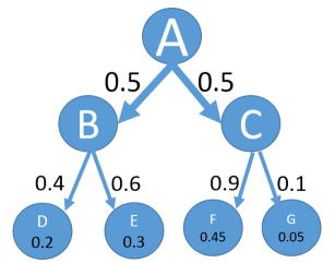
Figure 1: An example of the Dirichlet tree distribution.

Since microorganisms that are closely related often have similar functions, we can potentially better capture microbiome variation among samples by recognizing the structure among the observed features, which can be described using a taxonomic or phylogenetic tree structure. An extension of the Dirichlet distribution, the Dirichlet tree distribution (Dennis, 1991), can help us achieve this goal while maintaining conjugacy to the multinomial distribution. Figure 1 gives an example of the Dirichlet tree distribution, where the probability of a count being allocated to a leaf is the product of the branch probabilities leading to that leaf. When applied to model microbiome data, each tree node represents a taxonomy unit, and nodes closer to the top correspond to more generic or broad groupings. In the toy example shown in Figure 1, node A (the root node) could represent the kingdom Bacteria. We could then classify a random sequence as belonging to either phylum B or phylum C, each with 50% probability. If the sequence corresponds to phylum B, it could be further classified as belonging to class D with 40% probability or class E with 60% probability. Finer taxonomic or phylogenetic classification could be reflected by a tree with additional levels. While the Dirichlet multinomial distribution remains more commonly used to model microbiome data, the Dirichlet tree multinomial distribution has also been proposed in settings such as differential abundance testing and regression modeling (Wang and Zhao, 2017; Tang and Nicolae, 2017; Tang et al., 2018). To the best of our knowledge, we are the first to propose using the Dirichlet tree multinomial in the context of clustering.

We now describe some useful properties of the Dirichlet tree distribution in more detail. In particular, the Dirichlet tree distribution is conjugate to the multinomial distribution. To demonstrate this property, we can represent a multinomial sample as the outcome of a finite stochastic process. The probability of a count assigned to tree node $j$ being further classified to its child node $k$ is $b_{jk}$. Given the tree structure $T$ and the branch probabilities $B$ between nodes and their children, the probability of a single count $x$ can be written as $P(x|B,T)=\prod_{j\in J}\prod_{k\in K_{j}}b_{jk}^{\delta_{jk}(x)}$, where $J$ is the set of parent nodes, $K_{j}$ is the set of child nodes directly descending from node $j$ (not including any grandchildren or further descendants), and $\delta_{jk}(x)$ is the indicator of whether the count $x$ passes through the branch linking node $j$ and node $k$. For the branch probabilities $b_{jk}\in B,$ $b_{jk}>0$ for $j\in J,$ and $\sum_{k\in K_{j}}b_{jk}=1$. In this paper, we use $\mathbf{y}_{i}$ to denote the count vector for the $i$th observation, and $\mathbf{Y}$ to denote the corresponding count matrix for all the observations. Given the tree structure $T$ and the vector $\mathbf{y}_{i}$, one can compute the $|J|\times(|J|+d)$ matrix $X_{i}$ for the $i$th observation, where $|J|$ is the number of internal nodes of the tree and $d$ is the number of OTUs, i.e., leaf nodes of the tree. The matrix $X_{i}$ describes the number of counts traveling from parent nodes to children nodes. The collection of these matrices is denoted as $\mathbf{X}.$ The probability of the matrix of counts for the $i$th sample is:

$$P(X_{i}|B,T)=\prod_{j\in J}\frac{n_{j,.}(X_{i})!}{n_{j,1}(X_{i})!n_{j,2}(X_{i})!\dots n_{j,|K_{j}|}(X_{i})!}\prod_{k\in K_{j}}b_{jk}^{n_{j,k}(X_{i})},$$ (2)

where $n_{j,.}(X_{i})$ is the sum of the counts for all the nodes descending from node $j$ for the $i$th observation, $n_{j,k}(X_{i})$ is the number of counts descending from node $j$ to node $k$ for the $i$th observation, and $|K_{j}|$ is the number of children of node $j$.

A Dirichlet tree distribution can be expressed as a product of Dirichlet densities, $P(B)=\prod_{j\in J}p(\mathbf{b}_{j})$. If each $\mathbf{b}_{j}$ is given a Dirichlet prior, $P(\mathbf{b}_{j}|\alpha)=\mathrm{Dirichlet}(\alpha,\alpha,\dots,\alpha)$, one can obtain a Dirichlet tree multinomial distribution for observation $i$, after integrating out $B$:

$$\begin{split}P(X_{i}|T)=&\prod_{j\in J}\left[\frac{n_{j,.}(X_{i})!}{n_{j,1}(X_{i})!n_{j,2}(X_{i})!\dots n_{j,|K_{j}|}(X_{i})!}\cdot\right.\\ &\left.\prod_{k\in K_{j}}\frac{\Gamma(|K_{j}|\alpha)}{\{\Gamma(\alpha)\}^{|K_{j}|}}\frac{\{\prod_{k\in K_{j}}\Gamma(\alpha+n_{j,k}(X_{i}))\}}{\Gamma(|K_{j}|\alpha+\sum_{k\in K_{j}}n_{j,k}(X_{i}))}\right].\end{split}$$ (3)

2.2 Feature selection

In the current work, feature selection is achieved by identifying a parsimonious set of OTUs or tree nodes that exhibit differential abundance across groups. The rest of the features are not informative regarding the sample clustering, meaning that the corresponding parameters describing their relative abundance are not cluster-specific. To obtain a sparse model that selects informative OTUs or tree nodes, we introduce a binary vector $\boldsymbol{\gamma}$, whose entries indicate whether the corresponding features are useful in discriminating between sample groups, where $\gamma_{j}=1$ if $j$ is an informative feature and $0$ otherwise. For simplicity, we use a Bernoulli prior for $\boldsymbol{\gamma}$: $p(\boldsymbol{\gamma})\propto\prod_{j=1}^{d}w^{\gamma_{j}}(1-w)^{1-\gamma_{j}}$ (George and McCulloch, 1993; Madigan et al., 1995), where $d$ is the total number of features, and the prior probability of a feature being informative is $w$. In both the MFMDM and MFMDTM models, we select features that are relevant to clustering. We consider features not contributing to clustering as “noise” features, and features facilitating clustering as informative features.

2.2.1 Feature selection in the MFMDM model

In the proposed parsimonious model, the parameters describing the $i$th observation can be divided into a common part shared across all observations $p_{1},p_{2},...,p_{d-d_{\boldsymbol{\gamma}}}$, and a part specific to the cluster the $i$th observation belongs to, $w_{c_{i}}$, $q_{{c_{i}},1},q_{{c_{i}},2},...,q_{{c_{i}},d_{\boldsymbol{\gamma}}}$, where $c_{i}$ denotes the index of the cluster to which observation $i$ belongs, $d_{\boldsymbol{\gamma}}$ denotes the number of informative features, and $w_{c_{i}}$ controls the proportion of counts belonging to the informative features in cluster ${c_{i}}$. Each observation is modeled as a multinomial variable with parameters $\mathbf{y}_{i}\sim\mathrm{Multinomial}((1-w_{c_{i}})p_{1},(1-w_{c_{i}})p_{2},$ $\dots,$ $(1-w_{c_{i}})p_{d-d_{\boldsymbol{\gamma}}},w_{c_{i}}q_{{c_{i}},1},w_{c_{i}}q_{{c_{i}},2},\dots,$ $w_{c_{i}}q_{{c_{i}},d_{\boldsymbol{\gamma}}})$. In our notation, we reorder the elements of $\mathbf{y}_{i}$ such that the first $d-d_{\boldsymbol{\gamma}}$ elements are noisy and the remaining are informative, i.e., $\mathbf{y}_{i}=(\mathbf{y}_{ni},\mathbf{y}_{ei}).$

The length of the vectors $\boldsymbol{p}=(p_{1},p_{2},...,p_{d-d_{\boldsymbol{\gamma}}})$ and $\boldsymbol{q}_{c_{i}}=(q_{{c_{i}},1},q_{{c_{i}},2},...,q_{{c_{i}},d_{\boldsymbol{\gamma}}})$ will change with the number of OTUs selected as informative, but both $\boldsymbol{p}$ and $\boldsymbol{q}_{c_{i}}$ sum to $1$, thus guaranteeing the mean vector of the multinomial distribution will sum to $1$ as well. Finally, the likelihood for observation $i$ can be written as:

$$\begin{split}P(\mathbf{y}_{i}|c_{i},\boldsymbol{p},\boldsymbol{q}_{c_{i}},w_{c_{i}},\boldsymbol{\gamma})=&\frac{{\color[rgb]{0,0,0}y_{i,.}!}}{y_{n,i,1}!\dots y_{n,i,d-d_{\boldsymbol{\gamma}}}!y_{e,i,1}!\dots y_{e,i,d_{\boldsymbol{\gamma}}}!}\\ &{\color[rgb]{0,0,0}\times\{(1-w_{c_{i}})p_{1}\}^{y_{n,i,1}}\dots\{(1-w_{c_{i}})p_{d-d_{\boldsymbol{\gamma}}}\}^{y_{n,i,d-d_{\boldsymbol{\gamma}}}}}\\ &{\color[rgb]{0,0,0}\times(w_{c_{i}}q_{{c_{i}},1})^{y_{e,i,1}}\dots(w_{c_{i}}q_{{c_{i}},d_{\boldsymbol{\gamma}}})^{y_{e,i,d_{\boldsymbol{\gamma}}}}.}\end{split}$$ (4)

For observation $i$, $y_{n,i,j}$ is the number of counts of “noise” OTU $j$, $y_{e,i,l}$ is the number of counts of the informative OTU $l$, and $y_{i,.}=y_{n,i,.}+\ y_{e,i,.}$ is the total number of counts. The likelihood for all the observations is $P(\mathbf{Y}|\boldsymbol{p},\boldsymbol{q},\mathbf{w},\boldsymbol{\gamma},\mathbf{c})=\prod_{c\in C}\prod_{c_{i}=c}P(\mathbf{y}_{i}|c_{i},\boldsymbol{p},\boldsymbol{q}_{c_{i}},w_{c_{i}},\boldsymbol{\gamma})$, where $C$ denotes the set of distinct cluster indices.

In order to obtain a more tractable posterior distribution, we use the simplest conjugate priors by setting:

$$\begin{split}p_{1},p_{2},\dots,p_{d-d_{\boldsymbol{\gamma}}}&\sim\mathrm{Dirichlet}(\alpha,\alpha,\dots,\alpha)\\ q_{c,1},q_{c,2},\dots,q_{c,d_{\boldsymbol{\gamma}}}&\sim\mathrm{Dirichlet}(\alpha,\alpha,\dots,\alpha)\\ w_{c}&\sim\mathrm{Beta}(\beta_{1},\beta_{2}).\end{split}$$ (5)

For simplicity and objectivity, we assume all the parameters in the Dirichlet distribution are equal. Since our primary interest is in learning the cluster assignments and identifying discriminating features, we integrate out the remaining parameters to speed up computation. The resulting marginal likelihood is:

$$\begin{split}P(\mathbf{Y}|\boldsymbol{\gamma},\mathbf{c})=&\prod_{i=1}^{N}\frac{y_{i,.}!}{y_{n,i,1}!\dots y_{n,i,d-d_{\boldsymbol{\gamma}}}!y_{e,i,1}!\dots y_{e,i,d_{\boldsymbol{\gamma}}}{\color[rgb]{0,0,0}!}}\frac{\Gamma((d-d_{\boldsymbol{\gamma}})\alpha)}{\{\Gamma(\alpha)\}^{d-d_{\boldsymbol{\gamma}}}}\\ &\times\frac{\Gamma(\sum_{i=1}^{N}y_{n,i,1}+\alpha)\dots\Gamma(\sum_{i=1}^{N}y_{n,i,d-d_{\boldsymbol{\gamma}}}+\alpha)}{\Gamma(y_{n,.,.}+(d-d_{\boldsymbol{\gamma}})\alpha)}\\ &\times\prod_{c\in C}\frac{\Gamma(\beta_{1}+\beta_{2})}{\Gamma(\beta_{1})\Gamma(\beta_{2})}\frac{{\color[rgb]{0,0,0}\Gamma(\beta_{1}+\sum_{c_{i}=c}y_{e,i,.})\Gamma(\beta_{2}+\sum_{c_{i}=c}y_{n,i,.})}}{\Gamma(\beta_{1}+\beta_{2}+\sum_{c_{i}=c}y_{i,.})}\\ &\times\frac{\Gamma(d_{\boldsymbol{\gamma}}\alpha)}{\{\Gamma(\alpha)\}^{d_{\boldsymbol{\gamma}}}}\frac{\Gamma(\sum_{c_{i}=c}y_{e,i,1}+\alpha)\dots\Gamma(\sum_{c_{i}=c}y_{e,i,d_{\boldsymbol{\gamma}}}+\alpha)}{\Gamma(\sum_{c_{i}=c}y_{e,i,.}+d_{\boldsymbol{\gamma}}\alpha)}.\end{split}$$ (6)

2.2.2 Feature selection in the MFMDTM model

In the MFMDTM model, “noise” nodes’ allocation probabilities are the same across clusters. In contrast, informative nodes have cluster-specific allocation probabilities. We denote the set of informative parent nodes $J^{e}$, and the set of “noise” parent nodes $J^{n}$, with $J=J^{e}\cup J^{n}$. The MFMDTM method can therefore highlight the level within the tree structure where the sample composition begins to differentiate between clusters. This could be potentially advantageous when groups of microorganisms close together in the tree, which are typically functionally related, are up- or down-regulated in a coordinated manner.

We denote all the parameters associated with observation $i$ as $B_{i}$, with the part belonging to the “noise” nodes as $\mathbf{b}_{j}$, $j\in J^{n}$, and the part shared only by the observations in the same cluster $\mathbf{b}_{j}(c_{i})$, $j\in J^{e}$, $c_{i}\in\{1,2,\dots,C\}$. The likelihood of the vector of counts for the $i$th observation $X_{i}$ is:

$$\begin{split}P(X_{i}|B,T,\boldsymbol{\gamma},c_{i})=&\prod_{j}\frac{n_{j,.}(X_{i})!}{n_{j,1}(X_{i})!n_{j,2}(X_{i})!\dots n_{j,|K_{j}|}(X_{i})!}\\ &\prod_{j\in J^{n}}\prod_{k\in K_{j}}b_{jk}^{n_{j,k}(X_{i})}\prod_{j\in J^{e}}\prod_{k\in K_{j}}b_{jk}(c_{i})^{n_{j,k}(X_{i})}.\end{split}$$ (7)

The likelihood for the matrix of counts across all observations $\mathbf{X}$ is then:

$$\begin{split}P(\mathbf{X}|B,T,\boldsymbol{\gamma},C)=&\prod_{i}\left\{\prod_{j}\frac{n_{j,.}(X_{i})!}{n_{j,1}(X_{i})!n_{j,2}(X_{i})!\dots n_{j,|K_{j}|}(X_{i})!}\right\}\\ &\prod_{j\in J^{n}}\prod_{k\in K_{j}}b_{jk}^{n_{j,k}(\mathbf{X})}\prod_{c\in C}\prod_{j\in J^{e}}\prod_{k\in K_{j}}b_{jk}(c)^{n_{j,k}(\mathbf{X}^{c})}.\end{split}$$ (8)

Here $n_{j,k}(\mathbf{X})$ is the total number of counts descending from node $j$ to the $k$th child node for all the observations, $n_{j,k}(\mathbf{X}^{c})$ is the total number of counts descending from node $j$ to the $k$th child node for the observations in cluster $c$, $b_{j,k}$ is the probability of assigning count from non-informative node $j$ to its $k$th descending node, and $b_{j,k}(c)$ is the probability of assigning count from informative node $j$ to its $k$th descending node in cluster $c$.

Again, for simplicity of computation, we use the strategy of integrating out parameters. We consider the simplest conjugate prior $\mathbf{b}_{j}|\boldsymbol{\alpha}\sim\mathrm{Dirichlet}(\alpha,\alpha,\ldots,\alpha)$, and integrate out $B$. The marginal likelihood is:

$$\begin{split}P(\mathbf{X}|T,\boldsymbol{\gamma},\mathbf{c})=&\prod_{i}\left\{\prod_{j}\frac{n_{j,.}(X_{i})!}{n_{j,1}(X_{i})!n_{j,2}(X_{i})!\dots n_{j,|K_{j}|}(X_{i})!}\right\}\\ &\prod_{j\in J^{n}}\frac{\Gamma(|K_{j}|\alpha)}{\{\Gamma(\alpha)\}^{|K_{j}|}}\frac{(\prod_{k\in K_{j}}\Gamma(\alpha+n_{j,k}(\mathbf{X})))}{\Gamma(|K_{j}|\alpha+\sum_{k\in K_{j}}n_{j,k}(\mathbf{X}))}\\ &\prod_{c\in C}\prod_{j\in J^{e}}\frac{\Gamma(|K_{j}|\alpha)}{\{\Gamma(\alpha)\}^{|K_{j}|}}\frac{(\prod_{k\in K_{j}}\Gamma(\alpha+n_{j,k}(\mathbf{X}^{c})))}{\Gamma(|K_{j}|\alpha+\sum_{k\in K_{j}}n_{j,k}(\mathbf{X}^{c}))}.\end{split}$$ (9)

2.3 Mixture of finite mixtures

When the number of clusters is not prespecified, one can treat the data as arising from an infinite mixture of distributions, as in a Bayesian nonparametric approach such as the Dirichlet process mixture model. However, it has been shown that in a Dirichlet process mixture model, the number of clusters will grow with the number of observations (Miller and Harrison, 2014). Alternatively, one can treat the data as arising from a finite mixture of a given distribution and use methods such as reversible jump Markov chain Monte Carlo (RJMCMC) to learn the number of clusters from the data (Richardson and Green, 1997; Tadesse et al., 2005). Miller and Harrison (2018) proved that the MFM can consistently estimate the number of clusters, while the number of clusters in Dirichlet process mixtures will increase with sample size. They also demonstrated that efficient algorithms designed for the Dirichlet process mixture context can be applied for MFMs, avoiding the need for RJMCMC, which is notorious for being difficult to implement and computationally intensive. For this reason, we adopt the MFM in our modeling approach. The hierarchical formulation of our proposed model using the MFM framework is:

$$M \sim p_{m}, \text{where }p_{m}\text{ is a p.m.f on }\{1,2,\dots\},$$

$$(\pi_{1},\dots,\pi_{M})|M=m \sim\mathrm{Dirichlet}_{m}(\eta,\dots,\eta),$$

$$c_{1},\dots,c_{N}|\boldsymbol{\pi} \sim\mathrm{Categorical}(\boldsymbol{\pi}),$$

$$\boldsymbol{\gamma} \sim\prod_{j=1}^{d}\text{Bernoulli}(w),$$

$$\boldsymbol{\theta}\sim G_{00}, \quad\boldsymbol{\theta}_{1},\dots,\boldsymbol{\theta}_{M}\sim G_{0},$$

MFMDM model:

$$G_{0}|\boldsymbol{\gamma} =\text{Dirichlet}(\boldsymbol{\alpha}_{e}),$$

$$G_{00}|\boldsymbol{\gamma} =\text{Dirichlet}(\boldsymbol{\alpha}_{n}),$$

MFMDTM model:

$$G_{0}|\boldsymbol{\gamma} =\prod_{\gamma_{k}=1}\text{Dirichlet}(\boldsymbol{\alpha}_{k}),$$

$$G_{00}|\boldsymbol{\gamma} =\prod_{\gamma_{l}=0}\text{Dirichlet}(\boldsymbol{\alpha}_{l}),$$

$$\mathbf{X}_{i}|\boldsymbol{\theta}_{1:M},c_{1:N},\boldsymbol{\theta} \sim F(\boldsymbol{\theta}_{c_{i}},\boldsymbol{\theta}), \text{ for }i=1,\dots,N.$$

Here, $M$ is the underlying number of components in the population. The vector $\boldsymbol{\pi}=(\pi_{1},\dots,\pi_{M})$ is the probability of a random sample belonging to a component. $c_{1},\dots,c_{N}$ are the indices of the cluster to which each sample belongs. The vector $\boldsymbol{\gamma}$ is the feature selection indicator introduced in Section 2.2. $\boldsymbol{\theta}$ includes the parameters of the “noise” features, which are shared across all clusters, while $\boldsymbol{\theta}_{i}$ is the set of corresponding parameters for informative features of cluster $i$. For the MFMDM model, the distribution for $\boldsymbol{\theta}$ — $G_{00}$ and the base distribution for $\boldsymbol{\theta}_{m}$s — $G_{0}$, are two Dirichlet distributions, and the length of the parameter vectors correspond to the number of $0$ and $1$ elements in $\boldsymbol{\gamma}$ respectively. For the MFMDTM model, $G_{00}$ and $G_{0}$ are products of Dirichlet distributions, where the length of vector $\boldsymbol{\alpha}_{j}$ depends on the number of children nodes for node $j$. Without knowledge suggesting that informative features allocate counts more evenly (or less evenly) to their children than noisy features, we adopt the same prior for noisy features and informative features, with the purpose of facilitating a smooth transition between noisy and informative in the feature selection process. For simplicity, we let the parameter vectors of the Dirichlet distributions, including $\boldsymbol{\alpha}_{e}$, $\boldsymbol{\alpha}_{n}$ in the MFMDM model and $\boldsymbol{\alpha}_{j}$ in the MFMDTM model be vectors of $1$s for both $G_{0}$ and $G_{00}$. $F$ is the mixing kernel introduced in the above subsections, i.e., the multinomial distribution.

Similar to the Dirichlet process mixture model, the underlying discrete measure of the MFM model has a Pólya urn scheme representation, which enables sampling of the parameters for each observation sequentially. This close parallelism makes most sampling algorithms designed for the Dirichlet process mixture model directly applicable (Miller and Harrison, 2018). The parameter set for observation $i$, $\boldsymbol{\theta}_{i}$, will either take the identical value of an existing parameter, or a newly generated value from the base distribution $G_{0}$ with the following probability: $\boldsymbol{\theta}_{i}|\boldsymbol{\theta}_{-i}\sim\sum_{c\in C}(n_{c,-i}+\eta)\delta(\boldsymbol{\theta}_{c}^{*})+\frac{V_{N}(|C|+1)}{V_{N}(|C|)}\eta G_{0},$ where $\boldsymbol{\theta}_{-i}$ are the parameters for all the observations except for the $i$th observation; $\boldsymbol{\theta}_{c}^{*}$s are the distinct values of $\boldsymbol{\theta}_{-i}$, and $n_{c,-i}$s are the corresponding numbers of observations having the parameter $\boldsymbol{\theta}_{c}^{*}$, except for the $i$th observation. The function $V_{N}(R)$ is defined as $V_{N}(R)=\sum_{m=R}^{\infty}\frac{\Gamma(m+1)\Gamma(\eta m)}{\Gamma(m-R+1)\Gamma(\eta m+N)}p_{M}(m).$ This completes the specification of the MFMDM and MFMDTM models.

3 Method implementation

Obtaining a sample from the posterior distribution of either model requires the use of Markov chain Monte Carlo (MCMC). In each MCMC iteration, we first select OTUs or tree nodes by updating the latent indicator $\boldsymbol{\gamma}$ given the current cluster assignments, then fix $\boldsymbol{\gamma}$ and apply the split-and-merge algorithm to assign observations into clusters. Here we provide a high-level description of the algorithm, with additional details provided in the Supplementary Material.

3.1 Updates to feature selection indicators

The latent selection indicator $\boldsymbol{\gamma}$ is updated by repeating the following Metropolis step $t$ times, where $t=20$ following the suggestion of Kim et al. (2006). A new candidate $\boldsymbol{\gamma}^{new}$ is generated by randomly choosing one of the two transition moves:

1. add/delete by randomly picking one of the $d$ indices in $\boldsymbol{\gamma}^{old}$ and changing its value (from $0$ to $1$ or from $1$ to $0$);

2. swap by randomly drawing a 0 and a 1 in $\boldsymbol{\gamma}^{old}$ and switching their values.

The new candidate is accepted with probability $\min\left\{1,\frac{f(\boldsymbol{\gamma}^{new}|\mathbf{X},\mathbf{c})}{f(\boldsymbol{\gamma}^{old}|\mathbf{X},\mathbf{c})}\right\}$, where $\boldsymbol{c}$ is the cluster assignment vector. As $f(\boldsymbol{\gamma}|\mathbf{X},\boldsymbol{c})\propto f(\mathbf{X}|\boldsymbol{\gamma},\boldsymbol{c})\mathrm{P}(\boldsymbol{\gamma})$, the proposed acceptance probability can be calculated by:

$$\frac{f(\boldsymbol{\gamma}^{new}|\mathbf{X},\boldsymbol{c})}{f(\boldsymbol{\gamma}^{old}|\mathbf{X},\boldsymbol{c})}=\frac{f(\mathbf{X}|\boldsymbol{\gamma}^{new},\boldsymbol{c})\mathrm{P}(\boldsymbol{\gamma}^{new})}{f(\mathbf{X}|\boldsymbol{\gamma}^{old},\mathbf{c})\mathrm{P}(\boldsymbol{\gamma}^{old})}.$$ (10)

With the saved MCMC samples, one can calculate the marginal posterior inclusion probability vector $\boldsymbol{\pi}$ for all the features. For feature $i$, the posterior inclusion probability $\pi_{i}$ is the number of times feature $i$ was selected divided by the number of saved MCMC iterations. One could then rely on a pre-specified threshold as the cutoff for selection; a threshold of $0.5$ is a common choice, as it was shown to be optimal in the context of regression modeling (Barbieri and Berger, 2004). An alternative approach is to calculate the expected false discovery rate (FDR) from $\boldsymbol{\pi}$ and control the FDR to a target level. Further discussion is given in Section S4.1 of the Supplementary Material.

3.2 Updates to cluster assignments

We update the latent sample allocation vector $\boldsymbol{c}$ using Jain and Neal (2004)’s split-and-merge algorithm by first selecting two distinct observations, $i$ and $l$ uniformly at random. Let $\mathcal{C}$ denote the set of other observations that are in the same cluster with $i$ or $l$.

If $\mathcal{C}$ is empty, we use the simple random split-merge algorithm. Otherwise, we use the restricted Gibbs sampling split-merge algorithm. Both involve a Metropolis-Hastings sampling step, with acceptance probability:

$$a(\boldsymbol{c}^{merge},\mathbf{c})=\min\left\{1,\frac{q(\boldsymbol{c}|\boldsymbol{c}^{merge})\mathrm{P}(\boldsymbol{c}^{merge})L(\boldsymbol{c}^{merge}|\mathbf{X},\boldsymbol{\gamma})}{q(\boldsymbol{c}^{merge}|\boldsymbol{c})\boldsymbol{P}(\boldsymbol{c})L(\boldsymbol{c}|\mathbf{X},\boldsymbol{\gamma})}\right\}$$ (11)

if $c_{i}\neq c_{l}$, and

$$a(\mathbf{c}^{split}|\mathbf{c})=\min\left\{1,\frac{q(\boldsymbol{c}|\boldsymbol{c}^{split})\mathrm{P}(\mathbf{c}^{split})L(\mathbf{c}^{split}|\mathbf{X},\boldsymbol{\gamma})}{q(\boldsymbol{c}^{split}|\boldsymbol{c})\mathrm{P}(\boldsymbol{c})L(\boldsymbol{c}|\mathbf{X},\boldsymbol{\gamma})}\right\}$$ (12)

if $c_{i}=c_{l}$.

For the simple random split-merge algorithm, $\frac{q(\mathbf{c}|\mathbf{c}^{merge})}{q(\mathbf{c}^{merge}|\mathbf{c})}=1$, $\frac{q(\mathbf{c}|\mathbf{c}^{split})}{q(\mathbf{c}^{split}|\mathbf{c})}=1$. For the restricted Gibbs sampling, we first randomly create a launch state. This launch state is modified by a series of “intermediate” restricted Gibbs sampling steps to achieve a reasonable split of the observations. The last launch state is used for the calculation of the transient probabilities. Details on the split-and-merge algorithm and computing times are provided in the Supplementary Material.

The prior ratio, $\mathrm{P}(\mathbf{c}^{merge})/\mathrm{P}(\mathbf{c})$ or $\mathrm{P}(\mathbf{c}^{split})/\mathrm{P}(\mathbf{c})$, relies on the partition distribution $\mathrm{P}(\mathbf{c})$. In an MFM model, the probability function of $\mathbf{c}$ is $\mathrm{P}(\mathbf{c})=V_{N}(|C|)\prod_{c\in C}\eta^{(n_{c})}$. The probabilities of splitting a cluster and combining two clusters are:

$$\frac{\mathrm{P}(\mathbf{c}^{split})}{\mathrm{P}(\mathbf{c})} =\frac{V_{N}(|C|+1)}{V_{N}(|C|)}\frac{\Gamma(n_{c_{1}}+\eta)\Gamma(n_{c_{2}}+\eta)}{\Gamma(n_{c_{1}}+n_{c_{2}}+\eta)\Gamma(\eta)};$$ (13)

$$\frac{\mathrm{P}(\mathbf{c}^{merge})}{\mathrm{P}(\mathbf{c})} =\frac{V_{N}(|C|-1)}{V_{N}(|C|)}\frac{\Gamma(n_{c_{1}}+n_{c_{2}}+\eta)\Gamma(\eta)}{\Gamma(n_{c_{1}}+\eta)\Gamma(n_{c_{2}}+\eta)},$$ (14)

where $n_{c_{1}}$ and $n_{c_{2}}$ are the number of observations in the two clusters.

3.3 Post-processing of MCMC samples

The sampled values of the cluster indices can only describe whether two observations belong to the same cluster, but are not comparable between iterations, as the same index value may represent different clusters due to the “label switching” issue. In this paper, we adopt Fritsch and Ickstadt (2009)’s method for summarizing posterior cluster labels from MCMC samples. We denote the proposed clustering estimate as $c^{*}$, and estimate the probability that samples $i$ and $j$ belong to the same cluster from $M$ MCMC samples by $\zeta_{ij}=\frac{1}{M}\sum_{m=1}^{M}I(c_{i}^{(m)}=c_{j}^{(m)})$. A posterior cluster assignment can be obtained by maximizing the adjusted Rand index:

$$AR(c^{*},\zeta)=\frac{\sum_{i<j}\mathrm{I}_{\{c_{i}^{*}=c_{j}^{*}\}}\zeta_{ij}-\sum_{i<j}\mathrm{I}_{\{c_{i}^{*}=c_{j}^{*}\}}\sum_{i<j}\zeta_{ij}/{\color[rgb]{0,0,0}}}{\frac{1}{2}[\sum_{i<j}\mathrm{I}_{\{c_{i}^{*}=c_{j}^{*}\}}+\sum_{i<j}\zeta_{ij}]-\sum_{i<j}\mathrm{I}_{\{c_{i}^{*}=c_{j}^{*}\}}\sum_{i<j}\zeta_{ij}/{\color[rgb]{0,0,0}}}.$$ (15)

This method can handle the label-switching issue, and can be simply implemented using the R package “mcclust” (Fritsch, 2012).

4 Simulation studies

In this section, we first introduce the simulation setup, and then compare the performance of the proposed MFMDM and MFMDTM approaches with those from existing distance-based clustering methods, including PAM and hierarchical clustering (i.e., hcut) with complete linkage using the Euclidean, Bray Curtis, unweighted UniFrac, and weighted UniFrac distance metrics. For the completeness of comparison, the performances from the Dirichlet process mixture of Dirichlet (tree) multinomials (DPDM and DPDTM) are also included.

To construct the simulated data, we generated observations with structure similar to the dataset described in De Filippo et al. (2010). This study included two groups of samples, 14 from Africa and 15 from Italy. The original dataset has 2,803 OTUs with a median sequencing depth of 13,523. Due to the geographic distance and lifestyle difference between the two sample groups, we expect the microbiome profiles for the two groups to be well separated. We chose this dataset as the basis for our simulation study since their sequencing data is publicly available and the samples are well annotated. Also, it has a large number of OTUs with only a moderate number of observations, which is typical in microbiome data analysis. By relying on an existing microbiome dataset as the basis for our simulation study, we ensure that aspects of the simulated data such as the distribution of counts and shape of the tree structure resemble those in real data. In our simulation design, each group has 15 observations, and each observation has 15,000 total counts. We simulated 5 scenarios, with decreasing levels of complexity, and generate the OTU counts for the $z$th scenario, $z=1,2,\dots,5$, in the following way.

1. Choose two non-overlapping subsets of OTUs, $\Psi$ and $\Lambda$. In our simulation set-up, one subset $\Psi$ accounts for $13\%$ of the counts and $356$ OTUs, while the other subset $\Lambda$ accounts for $15\%$ of the counts and $595$ OTUs.

2. Set the expected abundance of the two groups using the marginal distributions. Let $\mathbf{p}_{\Psi}$ and $\mathbf{p}_{\Lambda}$ represent the vectors of marginal probabilities for the subsets $\Psi$ and $\Lambda$, respectively. For group A, we set the marginal probabilities for OTUs in subset $\Psi$ to $\mathbf{p}_{\Psi}^{A}=(1-z/5)\mathbf{p}_{\Psi}$, and correspondingly change the marginal probabilities for OTUs in subset $\Lambda$ to $\mathbf{p}_{\Lambda}^{A}=\mathbf{p}_{\Lambda}(\sum_{i\in\Lambda}p_{i}+z/5\sum_{i\in\Psi}p_{i})/\sum_{i\in\Lambda}p_{i}$. For group B, we change the marginal probabilities in the opposite direction, $\mathbf{p}_{\Psi}^{B}=(1+z/5)\mathbf{p}_{\Psi}$ and $\mathbf{p}_{\Lambda}^{B}=\mathbf{p}_{\Lambda}(\sum_{i\in\Lambda}p_{i}-z/5\sum_{i\in\Psi}p_{i})/\sum_{i\in\Lambda}p_{i}$.

3. Generate the count vectors from a Dirichlet multinomial with the sum of parameters to be $200$. The tree used in the MFMDTM model is the phylogenetic tree of the De Filippo dataset.

4. Repeat the above steps 200 times to generate 200 simulated data sets.

We now describe the parameter settings using in applying the proposed MFMDM and MFMDTM models. The parameters of the Beta distribution in the MFMDM model are set to be $\beta_{1}=\beta_{2}=1$, which corresponds to a uniform prior on the number of counts which are informative for clustering. Similarly, the parameters of the Dirichlet distribution for both the MFMDM and MFMDTM are set to be $\alpha=1$, which is a uniform prior in the multinomial case. The prior probabilities of OTUs being informative is $50\%$, i.e., $w=0.5$ for the MFMDM model. We give $M-1$ a $\mathrm{Poisson}(1)$ distribution, which expresses a preference for a small number of clusters. Sensitivity analyses regarding the choice of priors are included in the supplentary material S.3.

In both models, a large number of observed sequences inflates the factorial terms in the likelihood, which tends to support finer clusters. Unlike scale invariant mixtures (Malsiner-Walli et al., 2014), such as Gaussian mixtures, the likelihood of the Dirichlet (tree) multinomial is dependent on the number of sequences, which reflects both sequencing depth and rarefaction. To temper this effect and better achieve meaningful clustering, we take an approach similar to that of Grier et al. (2018) who “normalize” the data by first dividing the observed counts by a scaling parameter. For the simulated data, we found $50$ to be a reasonable scaling parameter. Based on our experiments with both simulated and real data, we found that the maximum sequencing depth divided by $300$ worked well for the choice of scaling parameter across all settings considered.

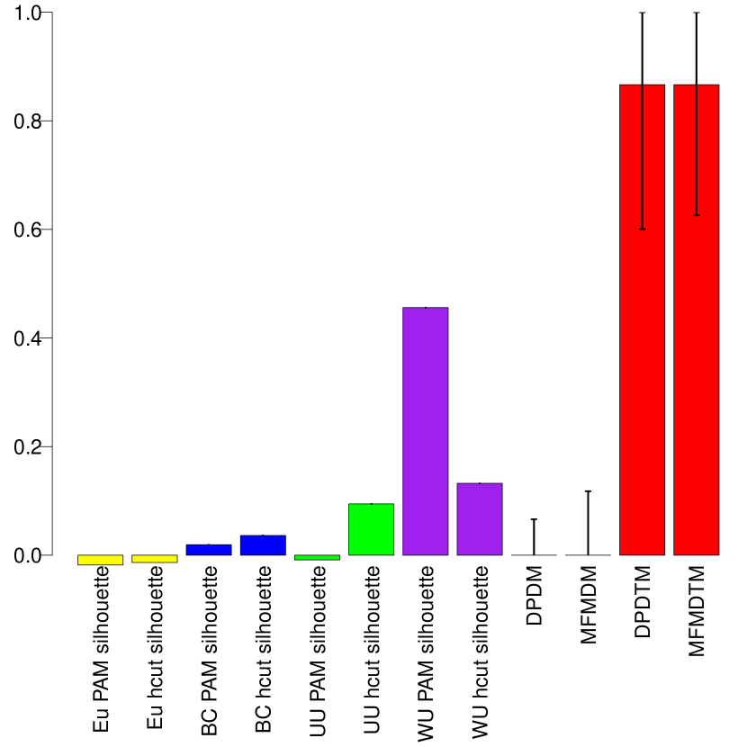
(a) Scenario 2

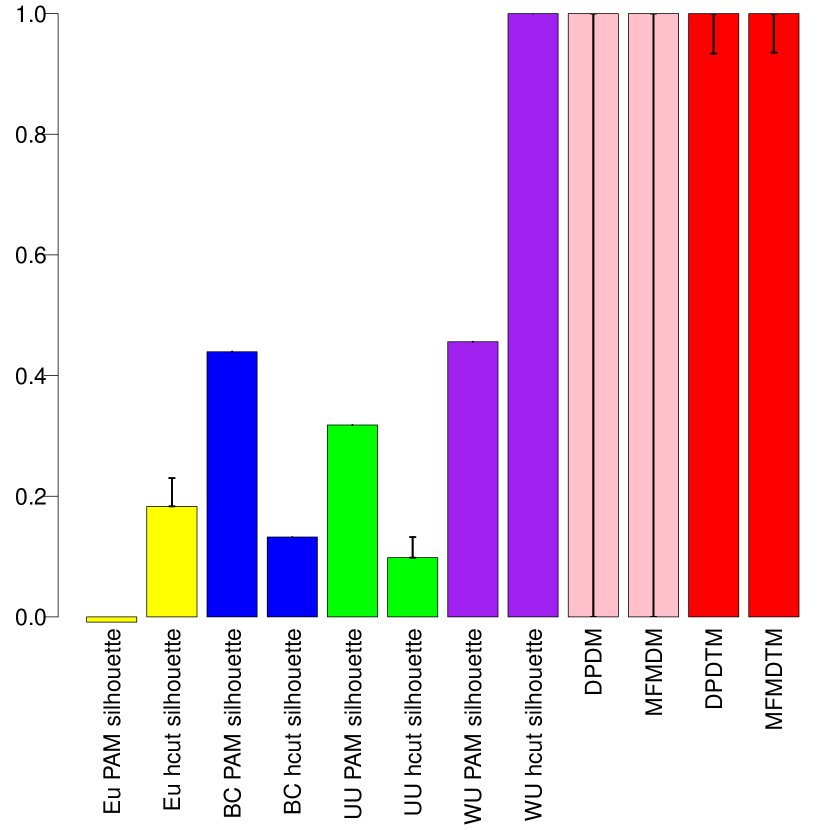
(b) Scenario 4

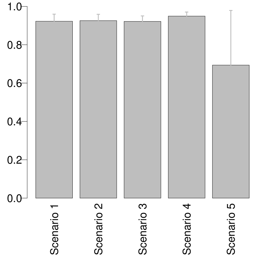
(c) OTU Selection AUC

Figure 2: Comparison with machine learning methods in terms of Rand indices, and the area under the curve (AUC) of the high abundance OTUs. The bar heights represent the median over 200 datasets, and the black intervals represent the empirical estimate of the $95\%$ confidence interval.

For each dataset, we run 20,000 iterations, the first 10,000 of which are discarded as burn-in, and then apply a thinning of $10$ and keep 1,000 samples for inference. For machine learning methods, the number of clusters is determined by the silhouette width, which is appropriate for non-Euclidean distances. We measure clustering performance using the adjusted Rand index. The expected value of the adjusted Rand index is 0 when clustering is done at random, while 1 reflects perfect recovery of the true underlying clusters in the data. Figure 2 (a) and (b) show the performance of our proposed methods, compared to some distance-based clustering methods for scenarios 2 and 4. Barplots for scenarios 1, 3, and 5 can be found in Supplementary Figure S1. Compared with the Dirichlet process mixture (DPM) model, the mixture of finite mixture (MFM) model can estimate the number of clusters consistently, i.e., the estimated number of clusters will not inflate with increased sample size. However, we found from our simulation studies that the performance of the DPM model and the MFM model is similar, which is in alignment with the empirical comparison in Miller and Harrison (2018), who observed that the two methods perform similarly on simulated datasets with moderate sample sizes. The main difference is the underlying belief: DPM assumes there are infinite number of mixture components, whereas MFM assumes finite number of mixture components. When the separation between the two clusters is relatively small, the proposed MFMDTM method, which performs variable selection accounting for the tree structure among features, shows a sizeable advantage over the distance-based methods including PAM using UniFrac distances, which incorporate phylogenetic information (Figure 2 (a)). When the separation between the clusters becomes larger, the performance of MFMDTM still shows significant improvement over that of competing methods that do not account for phylogeny (Figure 2 (b)). Though the empirical confidence interval is wide, the performance of the MFMDM model also improves significantly in this more separated scenario, achieving a median Rand index of 1. In general, the methods that incorporate tree information outperform those that do not, with MFMDTM achieving the highest adjusted Rand indices across all methods considered.

An advantage of the proposed methods over existing alternatives is that they enable the selection of informative features. The inference about informative vs. noisy features is based on the marginal posterior distribution of the latent indicator $\boldsymbol{\gamma}$, which is estimated from the selection frequencies in the MCMC output (Kim et al., 2006). It is worth mentioning that $\Psi$ and $\Lambda$ contain OTUs with low abundance, whose effects are negligible compared with the simulation noise. To set a meaningful goal for selection, we consider the $37$ high abundance OTUs that differ across groups, from among the $197$ high abundance OTUs in the dataset, as the true discriminatory features, where “high abundance” is defined as marginal abundance greater than $0.001$. For more details regarding feature selection under different thresholds, readers can refer to Supplementary Material Figure S9. As shown in Figure 2 (c), the area under the curve (AUC) values for the receiver operating curve (ROC) describing the accuracy of feature selection suggest that MFMDM’s selections are successful even when the Rand index is low. To provide intuition for this result, we note that achieving a high Rand index is a more challenging task than identifying influential features. To give an extreme example, the true cluster assignment is: two clusters with 15 observations each, however, the clustering algorithm concludes that there are two clusters, one with one observation while the other has 29 observations. The Rand index in this example is 0, but the features that separate one observation from the rest can still be the correct features that distinguish the two true clusters. The decrease in the AUC for Scenario 5 is due to the fact that the larger separation enables detection of informative OTUs that have marginal abundance below $0.001$, reducing the specificity. For five simulation scenarios, we show the ROC curves generated by varying the threshold on the posterior probability of feature inclusion of the 200 datasets in Supplementary Material Figure S10. These results show that the proposed method is able to accurately recover the informative features.

The proposed methods are fairly computationally intensive, but still feasible to run on a desktop computer. More specifically, for the simulated data described above, on a computer with an Intel Core i9-10900K 3.70GHz processor and 64GB memory, it takes Rcpp 14.58 minutes for 1000 MCMC iterations with the MFMDM model, and MATLAB R2020a 21.87 minutes for 1000 MCMC iterations with the MFMDTM model. We adopted a MATLAB implementation for the MFMDTM due to its simplicity in handling multi-dimensional arrays. The run time for the DPMDM model is similar to that of the MFMDM model (14.53 minutes). The difference in computation time between the MFM model and the DPM model is within $1\%$ of the total run time. Increasing the number of samples to 200 results in a run time of less than 2 hours for 1000 MCMC iterations.

5 Case study: tumor microbiome heterogeneity in pancreatic cancer

The goal of this case study is to provide insight into heterogeneity of the microbiome across pancreatic cancer patients. We rely on the data set described by Riquelme et al. (2019), which consists of microbiome profiles for 68 surgically resected PDAC samples. Among these 68 samples, 36 were obtained from long-term survivors, with survival times greater than 5 years, and 32 were obtained from stage-matched short-term survivors, who survived 5 years or less. Subjects were recruited from two cancer centers: The University of Texas MD Anderson Cancer Center (MDA, $n$ = 43) and Johns Hopkins University (JHU, $n$ = 25). The microbiome profiling data includes 2,410 OTUs corresponding to 1,095 taxonomic units at or above the species level.

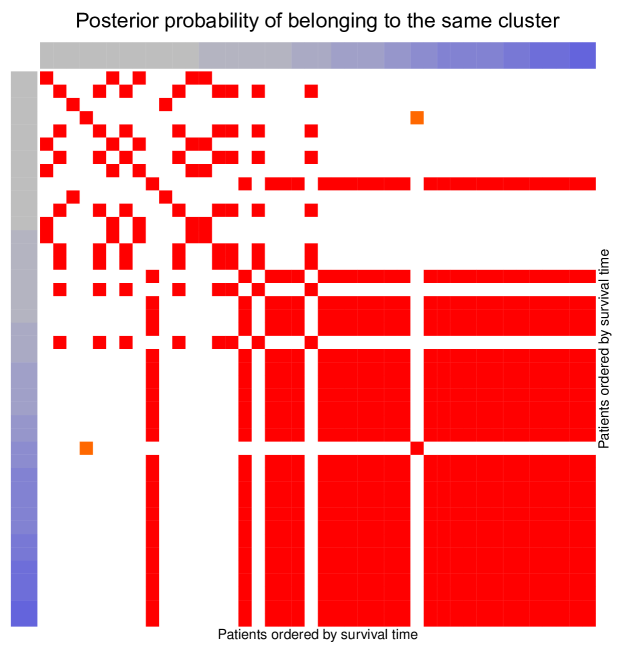
Figure 3: Heatmap showing the posterior probability of being assigned to the same cluster for patients with exact survival time for Riquelme et al. (2019) data. Patients are ordered by their survival times.

In order to uncover the natural sample groups and features driving these sample clusters, we applied the MFMDTM method to this data set, using the same parameter settings as in the simulation. For the MDA cohort, exact survival times were reported for 42 subjects, while for the JHU cohort, only a binary indicator of whether a patient survived more than 5 years was provided. For the patients with exact survival times, we plot a heatmap showing the posterior probability of any two observations belonging to the same cluster, where samples are sorted by survival time (Figure 3). The heatmap shows that long-term survivors cluster together with high probability, suggesting that their microbiome profiles are more consistent than that of short-term survivors. This finding suggests that it may be fruitful for researchers to investigate the specific bacteria present in long-term survivors, as reflecting a distinctive protective microbiome state. A similar conclusion can be drawn from the heatmap of all the samples using both the MFMDM and MFMDTM methods (Supplemental Figure S2). Our finding that long-term survivors consistently cluster together is particular interesting, since the long-term survivors came from two distinct geographic locations. Though some pre-clinical models (Pushalkar et al., 2018; Aykut et al., 2019) have suggested that certain microbial species are positively associated with tumor progression, our finding is aligned with that of Riquelme et al. (2019), who concluded that a protective microbiome induces anti-tumor immunity in long-term survivors and that those protective species are the key for future interventions.

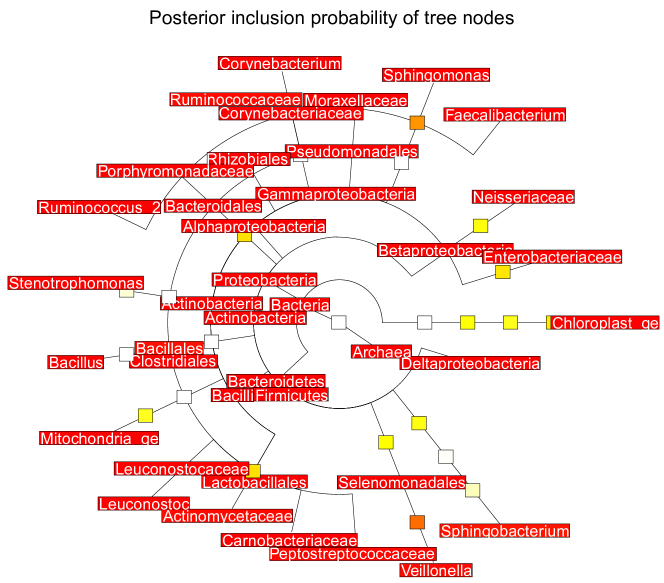
Figure 4: Posterior inclusion probabilities $\pi_{i}$ of the tree nodes for the Riquelme et al. (2019) data

Our model can also identify nodes in the taxonomic tree that drive the clustering of the samples. Figure 4 shows the nodes with high posterior inclusion probabilities in red, the majority of which were also identified in Riquelme et al. (2019). The original paper showed the predominance of Clostridia in short-term survivors and Alphaproteobacteria in long-term survivors at the class level, while our method shows that the two corresponding phyla, Firmicutes and Proteobacteria, are differential across clusters with posterior probability greater than $95\%$. Riquelme et al. (2019) identified the species Bacillus clausii as predictive of survivorship, and our method selects the genus it belongs to as a relevant feature. Some of the taxa identified our analysis using MFMDTM and the analysis by Riquelme et al. (2019) were discovered by previous research on PDAC. For example, Farrell et al. (2012) found that the abundance of the genus Corynebacterium is lower in PDAC patients than in healthy individuals, while our method specifically points out that the allocation probability for the family Corynebacteriaceae is differential across clusters. Geller et al. (2017) discovered that Proteobacteria producing cytidine deaminase are most associated with pancreatic cancer and our model identified several features under the phylum Proteobacteria, including the families Porphyromonadaceae and Enterobacteriaceae. In addition, MFMDTM identifies features that have not been thoroughly discussed in the pancreatic cancer literature before, such as the order Rhizobiales, which was found in higher abundance among patients with Helicobacter pylori-negative intestinal metaplasia than those with Helicobacter pylori-negative chronic superficial gastritis or cancer (Park et al., 2019).

Compared with the LEfSe method used in the original paper for differential abundance analysis Segata et al. (2011), which tends to select nested features, our method can identify the exact taxonomic level at which clusters are different. For completeness, we plot a heatmap showing the conditional probability of allocating a count to each child node for each selected parent node (Supplementary Figure S3) and a principal coordinate analysis (PCoA) plot of the samples colored by the MFMDTM cluster assignment (Supplement Figure S4).

6 Discussion

We have proposed two novel approaches for clustering of microbiome samples. Unlike existing approaches for microbiome clustering, our methods perform variable selection, which enables biological understanding of features that differentiate clusters present in the data, and does not require pre-specification of the number of clusters. The simulation results demonstrate that our methods can outperform commonly used unsupervised clustering algorithms in terms of the adjusted Rand index, suggesting that our sparse models are not only more interpretable but also more robust to noise.

Our application to tumor microbiome profiling of pancreatic cancer patients enhances the originally published analysis of this data set: while Riquelme et al. (2019) applied LefSe to identify microbiome features assuming known group membership, our approach shows that the long-term survivors make up a more natural cluster, while the short-term survivors are more heterogeneous, and our approach identifies additional features that are differential across the inferred clusters. These findings could guide the development of future microbiome interventions to improve cancer outcomes, which is an active and exciting area of current medical research (Reticker-Flynn and Engleman, 2019; McQuade et al., 2019). The Dirichlet multinomial mixture model code is included in the R package BayesianMicrobiome, while the Dirichlet tree multinomial mixture is implemented using Matlab. Both are available at https://github.com/YushuShi/sparseMbClust.

In this manuscript, we have largely focused on data obtained from 16S profiling. However, there is increasing interest in metagenomic whole genome sequencing (WGS) approaches, which allow for the comprehensive sequencing of all DNA present in a sample. While there are some differences between these two sequencing approaches, our methods are applicable to WGS data as well. More specifically, WGS can allow additional characterization of functional metabolic pathways by assigning the observed genetic sequences to biological roles, using tools such as HUMAnN2 or FMAP (Franzosa et al., 2018; Kim et al., 2016). Interestingly, these pathways can be organized into an ontological hierarchy (Caspi et al., 2013), making our tree-based clustering approach applicable in this context as well. The proposed methods can be scaled to hundreds of observations with several thousand features, as they exploit the conjugacy between the Dirichlet (tree) priors and multinomial distributions and rely on efficient Rcpp/Matlab implementations. If greater computational scalability is needed (for example, when applying the method to amplicon sequence variants obtained from WGS), a faster approach would be using variational inference to approximate the posterior. Variational inference for unsupervised clustering with simultaneous feature selection is an area that we would like to explore in our future research.

Finally, the proposed MFMDTM model assumes a fixed tree, but in reality, there may be uncertainty regarding the tree structure. One potential approach to incorporate uncertainty in the tree structure is to summarize the tree as a matrix of pairwise distances between the features (Zhang et al., 2021) and express the uncertainty of the tree structure through the variance of this matrix. The application of our methods to functional data derived from WGS and to settings with uncertainty regarding the tree structure are potential topics of interest in future work.

Data availability

The case study data was originally described in the publication Riquelme et al. (2019). Sequencing data and patient survival times can be accessed through the NCBI BioProject under Accession Number PRJNA542615. A processed version of the 16S data is available at https://github.com/YushuShi/sparseMbClust/, along with an R package implementing the Dirichlet multinomial mixture model code and Matlab code for the the Dirichlet tree multinomial mixture.

References

- Aykut et al. (2019) Aykut, B., Pushalkar, S., Chen, R., Li, Q., Abengozar, R. et al. (2019) The fungal mycobiome promotes pancreatic oncogenesis via activation of MBL. Nature, 574, 264–267.
- Barbieri and Berger (2004) Barbieri, M. M. and Berger, J. O. (2004) Optimal predictive model selection. The Annals of Statistics, 32, 870–897.
- Bray and Curtis (1957) Bray, J. and Curtis, J. (1957) An ordination of the upland forest communities of southern Wisconsin. Ecological Monographs, 27, 325–349.
- Caspi et al. (2013) Caspi, R., Dreher, K. and Karp, P. D. (2013) The challenge of constructing, classifying, and representing metabolic pathways. FEMS Microbiology Letters, 345, 85–93.
- Chen and Li (2013) Chen, J. and Li, H. (2013) Variable selection for sparse Dirichlet-Multinomial regression with an application to microbiome data analysis. The Annals of Applied Statistics, 7, 418–442.
- De Filippo et al. (2010) De Filippo, C., Cavalieri, D., Di Paola, M., Ramazzotti, M., Poullet, J., Massart, S., Collini, S., Pieraccini, G. and Lionetti, P. (2010) Impact of diet in shaping gut microbiota revealed by a comparative study in children from Europe and rural Africa. Proceedings of the National Academy of Sciences, 107, 14691–14696.
- Dennis (1991) Dennis, S. (1991) On the hyper-Dirichlet type 1 and hyper-Liouville distributions. Communications in Statistics-Theory and Methods, 20, 4069–4081.
- Fan et al. (2018) Fan, X., Alekseyenko, A. V., Wu, J., Peters, B. A., Jacobs, E. J., Gapstur, S. M., Purdue, M. P., Abnet, C. C., Stolzenberg-Solomon, R., Miller, G. et al. (2018) Human oral microbiome and prospective risk for pancreatic cancer: a population-based nested case-control study. Gut, 67, 120–127.
- Farrell et al. (2012) Farrell, J., Zhang, L., Zhou, H., Chia, D., Elashoff, D., Akin, D., Paster, B., Joshipura, K. and Wong, D. (2012) Variations of oral microbiota are associated with pancreatic diseases including pancreatic cancer. Gut, 61, 582–588. URL: https://gut.bmj.com/content/61/4/582.
- Franzosa et al. (2018) Franzosa, E., McIver, L., Rahnavard, G., Thompson, L., Schirmer, M. et al. (2018) Species-level functional profiling of metagenomes and metatranscriptomes. Nature Methods, 15, 962–968.
- Fritsch (2012) Fritsch, A. (2012) mcclust: Process an MCMC Sample of Clusterings. URL: https://CRAN.R-project.org/package=mcclust. R package version 1.0.
- Fritsch and Ickstadt (2009) Fritsch, A. and Ickstadt, K. (2009) Improved criteria for clustering based on the posterior similarity matrix. Bayesian Analysis, 4, 367–391. URL: https://doi.org/10.1214/09-BA414.
- Geller et al. (2017) Geller, L., Barzily-Rokni, M., Danino, T., Jonas, O., Shental, N., Nejman, D. et al. (2017) Potential role of intratumor bacteria in mediating tumor resistance to the chemotherapeutic drug gemcitabine. Science, 357, 1156–1160. URL: https://science.sciencemag.org/content/357/6356/1156.
- George and McCulloch (1993) George, E. and McCulloch, R. (1993) Variable selection via gibbs sampling. Journal of the American Statistical Association, 88, 881–889. URL: https://amstat.tandfonline.com/doi/abs/10.1080/01621459.1993.10476353.
- Grier et al. (2018) Grier, A., McDavid, A., Wang, B., Qiu, X., Java, J., Bandyopadhyay, S. et al. (2018) Neonatal gut and respiratory microbiota: coordinated development through time and space. Microbiome, 6, 193. URL: https://doi.org/10.1186/s40168-018-0566-5.
- Holmes et al. (2012) Holmes, I., Harris, K. and Quince, C. (2012) Dirichlet multinomial mixtures: Generative models for microbial metagenomics. PLOS One, 7, 1–15. URL: https://doi.org/10.1371/journal.pone.0030126.
- Jain and Neal (2004) Jain, S. and Neal, R. (2004) A split-merge Markov chain Monte Carlo procedure for the Dirichlet process mixture model. Journal of Computational and Graphical Statistics, 13, 158–182.
- Kaufman and Rousseeuw (2008) Kaufman, L. and Rousseeuw, P. (2008) Partitioning Around Medoids (Program PAM), chap. 2, 68–125. Wiley-Blackwell. URL: https://onlinelibrary.wiley.com/doi/abs/10.1002/9780470316801.ch2.
- Kim et al. (2016) Kim, J., Kim, M. S., Koh, A. Y., Xie, Y. and Zhan, X. (2016) FMAP: functional mapping and analysis pipeline for metagenomics and metatranscriptomics studies. BMC Bioinformatics, 17, 420.
- Kim et al. (2006) Kim, S., Tadesse, M. and Vannucci, M. (2006) Variable selection in clustering via Dirichlet process mixture models. Biometrika, 93, 877–893.
- Knight et al. (2017) Knight, R., Callewaert, C., Marotz, C., Hyde, E., Debelius, J., McDonald, D. and Sogin, M. (2017) The microbiome and human biology. Annual Review of Genomics and Human Genetics, 18, 65–86.
- Lozupone et al. (2007) Lozupone, C., Hamady, M., Kelley, S. and Knight, R. (2007) Quantitative and qualitative diversity measures lead to different insights into factors that structure microbial communities. Applied and Environmental Microbiology, 73, 1576–1585.
- Lozupone and Knight (2005) Lozupone, C. and Knight, R. (2005) Unifrac: a new phylogenetic method for comparing microbial communities. Applied and Environmental Microbiology, 71, 8228–8235.
- MacQueen (1967) MacQueen, J. (1967) Some methods for classification and analysis of multivariate observations. In Proceedings of the fifth Berkeley symposium on mathematical statistics and probability, vol. 1, 281–297. Oakland, CA, USA.
- Madigan et al. (1995) Madigan, D., York, J. and Allard, D. (1995) Bayesian graphical models for discrete data. International Statistical Review / Revue Internationale de Statistique, 63, 215–232. URL: http://www.jstor.org/stable/1403615.
- Malsiner-Walli et al. (2014) Malsiner-Walli, G., Frühwirth-Schnatter, S. and Grün, B. (2014) Model-based clustering based on sparse finite gaussian mixtures. Statistics and Computing, 26, 303–324.
- McQuade et al. (2019) McQuade, J., Daniel, C., Helmink, B. and Wargo, J. (2019) Modulating the microbiome to improve therapeutic response in cancer. The Lancet Oncology, 20, e77–e91.
- Miller and Harrison (2014) Miller, J. and Harrison, M. (2014) Inconsistency of Pitman-Yor process mixtures for the number of components. Journal of Machine Learning Research, 15, 3333–3370. URL: http://jmlr.org/papers/v15/miller14a.html.
- Miller and Harrison (2018) — (2018) Mixture models with a prior on the number of components. Journal of the American Statistical Association, 113, 340–356. URL: https://doi.org/10.1080/01621459.2016.1255636.
- Mizrahi et al. (2020) Mizrahi, J. D., Surana, R., Valle, J. W. and Shroff, R. T. (2020) Pancreatic cancer. The Lancet, 395, 2008–2020.
- Park et al. (2019) Park, C., Lee, A., Lee, Y., Eun, C., Lee, S. and Han, D. (2019) Evaluation of gastric microbiome and metagenomic function in patients with intestinal metaplasia using 16S rRNA gene sequencing. Helicobacter, 24, e12547. URL: https://onlinelibrary.wiley.com/doi/abs/10.1111/hel.12547.
- Pushalkar et al. (2018) Pushalkar, S., Hundeyin, M., Daley, D., Zambirinis, C., Kurz, E. et al. (2018) The pancreatic cancer microbiome promotes oncogenesis by induction of innate and adaptive immune suppression. Cancer Discovery, 8, 403–416.
- Reticker-Flynn and Engleman (2019) Reticker-Flynn, N. and Engleman, E. (2019) A gut punch fights cancer and infection. Nature, 565, 573–574.
- Richardson and Green (1997) Richardson, S. and Green, P. (1997) On Bayesian analysis of mixtures with an unknown number of components (with discussion). Journal of the Royal Statistical Society: series B (statistical methodology), 59, 731–792.
- Riquelme et al. (2019) Riquelme, E., Zhang, Y., Zhang, L., Montiel, M., Zoltan, M., Dong, W. et al. (2019) Tumor microbiome diversity and composition influence pancreatic cancer outcomes. Cell, 178, 795 – 806.e12. URL: http://www.sciencedirect.com/science/article/pii/S0092867419307731.
- Rousseeuw (1987) Rousseeuw, P. (1987) Silhouettes: A graphical aid to the interpretation and validation of cluster analysis. Journal of Computational and Applied Mathematics, 20, 53–65. URL: http://www.sciencedirect.com/science/article/pii/0377042787901257.
- Segata et al. (2011) Segata, N., Izard, J., Waldron, L., Gevers, D., Miropolsky, L., Garrett, W. S. and Huttenhower, C. (2011) Metagenomic biomarker discovery and explanation. Genome Biology, 12, 1–18.
- Tadesse et al. (2005) Tadesse, M., Sha, N. and Vannucci, M. (2005) Bayesian variable selection in clustering high-dimensional data. Journal of the American Statistical Association, 100, 602–617.
- Tang et al. (2018) Tang, Y., Ma, L. and Nicolae, D. (2018) A phylogenetic scan test on a Dirichlet-tree multinomial model for microbiome data. The Annals of Applied Statistics, 12, 1–26. URL: https://doi.org/10.1214/17-AOAS1086.
- Tang and Nicolae (2017) Tang, Y. and Nicolae, D. L. (2017) Mixed effect Dirichlet-tree Multinomial for longitudinal microbiome data and weight prediction.
- Wadsworth et al. (2017) Wadsworth, W. D., Argiento, R., Guindani, M., Galloway-Pena, J., Shelburne, S. A. and Vannucci, M. (2017) An integrative Bayesian Dirichlet-multinomial regression model for the analysis of taxonomic abundances in microbiome data. BMC Bioinformatics, 18, 1–12.
- Wang and Zhao (2017) Wang, T. and Zhao, H. (2017) A Dirichlet-tree multinomial regression model for associating dietary nutrients with gut microorganisms. Biometrics, 73, 792–801.
- Wei et al. (2019) Wei, M., Shi, S., Liang, C., Meng, Q., Hua, J., Zhang, Y., Liu, J., Zhang, B., Xu, J. and Yu, X. (2019) The microbiota and microbiome in pancreatic cancer: more influential than expected. Molecular Cancer, 18, 97.
- Zhang et al. (2021) Zhang, L., Shi, Y., Jenq, R. R., Do, K.-A. and Peterson, C. B. (2021) Bayesian compositional regression with structured priors for microbiome feature selection. Biometrics, 77, 824–838. URL: https://onlinelibrary.wiley.com/doi/abs/10.1111/biom.13335.