Eulerian dynamics in multi-dimensions with radial symmetry

Abstract.

We study the global wellposedness of pressure-less Eulerian dynamics in multi-dimensions, with radially symmetric data. Compared with the 1D system, a major difference in multi-dimensional Eulerian dynamics is the presence of the spectral gap, which is difficult to control in general. We propose a new pair of scalar quantities that provides a significant better control of the spectral gap. Two applications are presented. (i) the Euler-Poisson equations: we show a sharp threshold condition on initial data that distinguish global regularity and finite time blowup; (ii) the Euler-alignment equations: we show a large subcritical region of initial data that leads to global smooth solutions.

1. Introduction

We consider the following pressure-less Euler equation with forces

$$\partial_{t}\rho+\nabla\cdot(\rho\mathbf{u})=0,$$ (1)

$$\partial_{t}(\rho\mathbf{u})+\nabla\cdot(\rho\mathbf{u}\otimes\mathbf{u})=\rho\mathbf{F},$$ (2)

subject to the initial condition

$$\rho(\mathbf{x},t=0)=\rho_{0}(\mathbf{x}),\quad\mathbf{u}(\mathbf{x},t=0)=\mathbf{u}_{0}(\mathbf{x}).$$ (3)

Here, $\rho:\mathbb{R}^{n}\times\mathbb{R}_{+}\to\mathbb{R}$ represents the density of the fluid, and $\mathbf{u}:\mathbb{R}^{n}\times\mathbb{R}_{+}\to\mathbb{R}^{n}$ is the flow velocity. $\mathbf{F}$ is a general forcing acting on the flow. It could depend on $\rho$ and $\mathbf{u}$.

The Eulerian dynamics (1)-(2) is a fundamental system of equations in fluid mechanics. It has a vast amount of applications with different choices of forces $\mathbf{F}$. A big challenging and demanding question is to understand whether the solutions are globally regular, or there could be singularity formations in finite time.

1.1. Spectral dynamics and the spectral gap

The momentum equation (2) can be equivalently written as the following dynamics of the velocity $\mathbf{u}$, in the non-vacuous region

$$\partial_{t}\mathbf{u}+(\mathbf{u}\cdot\nabla)\mathbf{u}=\mathbf{F}.$$ (4)

When $\mathbf{F}\equiv 0$, (4) is the classical inviscid Burgers equation. It is well-known that the solution admits a finite time shock formation, for any generic smooth initial data. Indeed, in one dimension, taking $x$-derivative of the equation, one immediately obtain $(\partial_{t}+u\partial_{x})(\partial_{x}u)=-(\partial_{x}u)^{2}$. This yields a Ricatti equation of $\partial_{x}u$ along the characteristic paths, which governs the main structure of the solution: blowup happens in finite time if initially $\partial_{x}u_{0}(x)<0$. The idea of tracing the dynamics of $\partial_{x}u$ also works very well for 1D models of the type (4), with different forcing terms.

In multi-dimensions, taking the spatial gradient of (4) would yield

$$(\partial_{t}+\mathbf{u}\cdot\nabla)\nabla\mathbf{u}=-(\nabla\mathbf{u})^{\otimes 2}+\nabla\mathbf{F},$$ (5)

where the velocity gradient $\nabla\mathbf{u}$ is an $n$-by-$n$ matrix. In many applications, the boundedness of $\nabla\mathbf{u}$ plays a crucial role in the propagation of the regularity of the solution. A natural question would be

Which scalar quantities exhibit the same Ricatti structure as $\partial_{x}u$ in 1D?

One candidate is the set of eigenvalues of $\nabla\mathbf{u}$, denoted by $\{\lambda_{i}\}_{i=1}^{n}$. Indeed, when $\mathbf{F}\equiv 0$, the dynamics of $\lambda_{i}$, known as the spectral dynamics, satisfies the same Ricatti equation as 1D: $(\partial_{t}+\mathbf{u}\cdot\nabla)\lambda_{i}=-\lambda_{i}^{2}$. It can be solved explicitly along the characteristic paths, deducing a similar blowup phenomenon, despite of the fact that $\lambda_{i}$ could be complex-valued.

With the forcing term, the spectral dynamics of (5) has the form

$$(\partial_{t}+\mathbf{u}\cdot\nabla)\lambda_{i}=-\lambda_{i}^{2}+l_{i}^{T}(\nabla\mathbf{F})r_{i},\quad i=1,\cdots,n,$$ (6)

where $(l_{i},r_{i})$ are the corresponding left and right eigenvectors of $\lambda_{i}$. It has been studied extensively in [12]. Although one can largely benefit from the explicit Ricatti structure, it is in general hard to control $l_{i}^{T}(\nabla\mathbf{F})r_{i}$, as in many cases $\nabla\mathbf{F}$ does not share the same eigenvectors with $\nabla\mathbf{u}$.

Another natural replacement of $\partial_{x}u$ in multi-dimensions would be the divergence

$$d:=\nabla\cdot\mathbf{u}=\text{tr}(\nabla\mathbf{u})=\sum_{i=1}^{n}\lambda_{i},$$

whose dynamics can be obtained by taking the trace of (6). It reads

$$(\partial_{t}+\mathbf{u}\cdot\nabla)d=-\text{tr}\left((\nabla\mathbf{u})^{\otimes 2}\right)+\nabla\cdot\mathbf{F}.$$

Investigating the dynamics of $d$ has a couple of advantages. First, $d$ is real-valued. More importantly, it is more friendly to the forcing term, as $\nabla\cdot\mathbf{F}$ is much easier to handle (compared with $l_{i}^{T}(\nabla\mathbf{F})r_{i}$) in many applications.

However, the term $\text{tr}\left((\nabla\mathbf{u})^{\otimes 2}\right)\neq d^{2}$, for $n\geq 2$. The difference is related to the spectral gap of the matrix $\nabla\mathbf{u}$, defined as

$$\eta=\frac{1}{2}\sum_{i=1}^{n}\sum_{j=1}^{n}(\lambda_{i}-\lambda_{j})^{2}.$$ (7)

Indeed, it is easy to check that the difference

$$d^{2}-\text{tr}\left((\nabla\mathbf{u})^{\otimes 2}\right)=\frac{n-1}{n}d^{2}-\frac{1}{n}\,\eta.$$ (8)

Therefore, to make use of the Ricatti structure and to extend 1D regularity results to multi-dimensions, one needs to additionally control the spectral gap, which turns out to be a difficult task. As we will argue in Remark 2.5, $\nabla\cdot\mathbf{u}$ might not be a good replacement for $\partial_{x}u$, due to the presence of the spectral gap.

In the following, we focus on two classical models on Eulerian dynamics with nonlocal interaction forces.

1.2. The Euler-Poisson equations

The Euler-Poisson equations is a fundamental system in plasma physics. It describes the electron fluid interacting with its own electric field against a charged ion background [7]. The pressure-less Euler-Poisson equations have the form (1)-(2), with the force

$$\mathbf{F}=-\kappa\nabla(-\Delta)^{-1}(\rho-c),$$ (9)

where the parameter $\kappa$ denotes the strength of the charge force, and $c\geq 0$ is a constant background.

The 1D Euler-Poisson equation has been studied extensively in [5], where a sharp critical threshold on the initial data is obtained that distinguishes the global wellposedness of solutions and the finite-time singularity formations. The result is extended to the system with pressure in [19].

However, in higher dimensions, global wellposedness remains to be a challenging open problem. In the case where pressure is presented, global solutions can be obtained for small initial data perturbed from a constant state [7, 11], leveraging the dispersive structure. For the pressureless system, very little is known, even for small initial data. The main difficulty on the spectral analysis (6) is that

$$\nabla\mathbf{F}=-\kappa\nabla\otimes\nabla(-\Delta)^{-1}(\rho-c)$$

is a nonlocal Reisz transform on $\rho$, which is hard to control.

An important observation is that, $\nabla\cdot\mathbf{F}=\kappa(\rho-c)$ depends only on local information of $\rho$. Therefore, the force is more friendly when tracing the dynamics of the divergence

$$d^{\prime}=-\text{tr}\left((\nabla\mathbf{u})^{\otimes 2}\right)+\kappa(\rho-c).$$

This approach has been studied in [17]. Although the forcing term is much easier to handle, the major difficulty is shifted to the control of the spectral gap (7), which depends non-locally on $\rho$ and $d$. A restricted Euler-Poisson (REP) equation is introduced in [17], with modifications on the $\text{tr}\left((\nabla\mathbf{u})^{\otimes 2}\right)$ term so that the spectral gap becomes locally dependent on $\rho$. However, the result can not be easily extended to the Euler-Poisson equations due to the lack of control on the spectral gap.

1.3. The Euler-alignment equations

Another model of Eulerian dynamics is called the Euler-alignment system, where

$$\mathbf{F}=\int\phi(\mathbf{x}-\mathbf{y})(\mathbf{u}(\mathbf{y},t)-\mathbf{u}(\mathbf{x},t))\rho(\mathbf{y},t)\,d\mathbf{y}.$$ (10)

It is the macroscopic representation of the Cucker-Smale model [3], describing the emergent behavior in animal flocks. The $\mathbf{F}$ is called a nonlocal alignment force, where $\phi$ is the influence function that measures the strength of the influence between a pair of agents. The Euler-alignment system was first introduced and formally derived in [8], with rigorous justifications in [6].

The Euler-alignment system has been studied in [18]. The result contains threshold conditions on initial data which leads to global regularity or finite-time singularity formations, in both 1D and 2D. In particular, the 2D result is obtained by tracing the dynamics of $d$, together with a control of the spectral gap. The conditions are not sharp, due to the non-locality of the alignment force.

In a successive work [1], a remarkable commutator structure in $\mathbf{F}$ was discovered, which leads to a sharp critical threshold that distinguishes global regularity and finite time blowup of the solutions, for the system in 1D. It also reveals intriguing connections to other models in fluid mechanics. Then, theories on global solutions are developed in 1D for different types of influence functions, including strongly singular alignment [4, 16], weakly singular alignment [20], as well as misalignment [14]. Different behaviors are observed in each case. In particular, with strongly singular alignment, the system becomes dissipative, and all smooth non-vacuous initial data leads to global regularity. All 1D results are sharp.

For the multi-dimensional Euler-alignment system, much less is known in regards to global regularity. In [9], improved threshold conditions are derived in 2D, taking advantage of the commutator structure, which turns out to be the same as 1D in the dynamics of $d$. However, the result is far from optimal, as one needs to additionally control the spectral gap. With strongly singular alignment, global regularity is proved in [15], for small initial data near the steady state. The result is much weaker than 1D. The smallness condition is used to control the spectral gap.

The two models above are two examples of Eulerian dynamics, where the global regularity theory is much less developed in multi-dimensions, compared with one-dimension. The major difficulty is to control the effect of the spectral gap.

In this paper, we study the Eulerian dynamics with radially symmetric initial data. Despite the redial symmetry, the effect of the spectral gap still persists (see (14)). We propose a new pair of scalar quantities as the replacement of $\partial_{x}u$ in 1D. Compared with $\{\lambda_{i}\}_{i=1}^{n}$, the quantities are real-valued, and are more friendly to the forcing term. Compared with $d$, the dynamics of the quantities have the precise Ricatti structure, so we can avoid a direct nonlocal control of the spectral gap.

The newly proposed quantities allow us to obtain significantly better regularity results for Eulerian dynamics in multi-dimensions with radial symmetry. We apply the idea to the Euler-Poisson and the Euler-alignment equations. Further extension can be made to a large class of Eulerian dynamics with different forcing terms.

For the Euler-Poisson equations, we obtain a sharp threshold condition, stated in Theorem 2.6. This is the first sharp result on the Euler-Poisson system in multi-dimensions for all smooth radially symmetric initial data (see Remark 2.7 for more discussions). For the Euler-alignment equations, we show global regularity with a large region of initial data, in Theorem 2.8. Although the result is not sharp, it significantly improves the existing results in the literature (see Remark 2.9).

The rest of the paper is organized as follows. In section 2, we introduce the new scalar quantities, and state our main results. We will then discuss the Euler-Poisson equations and the Euler-alignment equations in sections 3 and 4 respectively. We end the paper with some further discussion in section 5.

2. Radially symmetric solutions and the new scalar quantities

We focus on a special type of solutions for the Eulerian dynamics (1)-(2), with radial symmetry and without swirl

$$\rho(\mathbf{x},t)=\rho(r,t),\quad\mathbf{u}(\mathbf{x},t)=\frac{\mathbf{x}}{r}u(r,t).$$ (11)

Here, $r=|\mathbf{x}|\in\mathbb{R}_{+}$ is the radial variable. $\rho$ and $u$ are scalar functions defined in $\mathbb{R}_{+}\times\mathbb{R}_{+}$. Appropriate boundary conditions at $r=0$ are assumed, to ensure regularity of $\rho$ and $\mathbf{u}$ at the origin, for instance, $u(0,t)=0$, $\partial_{r}\rho(0,t)=0$. In all examples that we concern, the force takes the form

$$\mathbf{F}(\mathbf{x},t)=\frac{\mathbf{x}}{r}F(r,t).$$ (12)

So, the radial symmetry is preserved in time.

Our goal is to find appropriate scalar quantities that serve as the multi-dimensional replacement of $\partial_{x}u$ that exhibit the Ricatti structure, and meanwhile help us control the spectral gap $\eta$ as well as the force $F$.

Let us first calculate the divergence

$$d=\nabla\cdot\mathbf{u}=u_{r}+(n-1)\frac{u}{r},$$ (13)

and the difference in (8) (representing the spectral gap $\eta$)

$$d^{2}-\text{tr}\left((\nabla\mathbf{u})^{\otimes 2}\right)=2(n-1)u_{r}\frac{u}{r}+(n-1)(n-2)\frac{u^{2}}{r^{2}}.$$ (14)

Clearly, the term in (14) does not vanish in the radially symmetric setup, and can not be determined by local information in $d$.

A remarkable observation is that, both the divergence and the difference can be determined by local information of the two quantities $u_{r}$ and $\frac{u}{r}$. In fact, the spectral gap $\eta=\frac{1}{n-1}(u_{r}-\frac{u}{r})^{2}$.

Hence, we propose to use the pair

$$(p,q):=\left(u_{r},\frac{u}{r}\right)$$ (15)

as the multi-dimensional replacement of $\partial_{x}u$.

Note that the boundedness of the pair (15) is equivalent to the boundedness of $\nabla\mathbf{u}$, the quantities that play a crucial role in preserving the regularity of the solution.

Proposition 2.1.

Suppose $u_{r}$ and $\frac{u}{r}$ are bounded. Then, $\nabla\mathbf{u}$ is bounded.

Proof.

It follows from the direct computation

$$\partial_{x_{j}}u_{i}=\frac{x_{i}x_{j}}{r^{2}}u_{r}+\left(\delta_{ij}-\frac{x_{i}x_{j}}{r^{2}}\right)\frac{u}{r},$$

where $\delta_{ij}$ is the Kronecker delta. ∎

In the following, we argue that the pair (15) is a better replacement of $\partial_{x}u$, compared with $\{\lambda_{i}\}_{i=1}^{n}$ and $d$. We proceed with four examples: the inviscid Burgers equation, the damped Burgers equation, the Euler-Poisson equations, and the Euler-alignment equations.

2.1. The inviscid Burgers equation

Consider the inviscid Burgers equation (4) with $\mathbf{F}\equiv 0$

$$\mathbf{u}_{t}+(\mathbf{u}\cdot\nabla)\mathbf{u}=0,$$

under the radially symmetric setup (11). The dynamics of the pair (15) reads

$$\begin{cases}p^{\prime}=-p^{2},\\ q^{\prime}=-q^{2},\end{cases}$$

where ${}^{\prime}=\partial_{t}+u\partial_{r}$ denotes the material derivative. It is a decoupled system, with two Ricatti equations the same as (6). This immediately implies a sharp global regularity result.

Theorem 2.2.

The solution of the radially symmetric inviscid Burgers equation is globally regular, if and only if

$$u^{0}_{r}(r)\geq 0,\quad\text{and}\quad\frac{u^{0}(r)}{r}\geq 0.$$

Proof.

The Ricatti structure implies that $(p,q)$ are uniformly bounded in time if and only if the condition holds. Global regularity then follows from Proposition 2.1 and the classical equivalency between boundedness of $\nabla\mathbf{u}$ and global regularity. ∎

Remark 2.3.

From (13), we know the divergence $d$ is a linear combination of $(p,q)$. However, due to the nonlinear evolution of $(p,q)$, we have

$$d^{\prime}=p^{\prime}+(n-1)q^{\prime}=-p^{2}-(n-1)q^{2}\neq-d^{2},$$

and the difference (14) can not be expressed locally in terms of $d$, and additional nonlocal control is required on the spectral gap. This indicates the advantage of studying the pair $(p,q)$ compared with the divergence $d$.

2.2. The damped Burgers equation

Let us consider another example (4), with a damping force $\mathbf{F}=-\kappa\mathbf{u}$. This corresponds to the damped Burgers equation

$$\mathbf{u}_{t}+(\mathbf{u}\cdot\nabla)\mathbf{u}=-\kappa\mathbf{u}.$$ (16)

Similarly, one can obtain the dynamics of the pair (15) under the radial symmetric setup

$$\begin{cases}p^{\prime}=-p^{2}-\kappa p,\\ q^{\prime}=-q^{2}-\kappa q.\end{cases}$$

Solving the decoupled system, we obtain

Theorem 2.4.

The radially symmetric solutions of the damped Burgers equation (16) are globally regular, if and only if

$$u^{0}_{r}(r)\geq-\kappa,\quad\text{and}\quad\frac{u^{0}(r)}{r}\geq-\kappa.$$ (17)

Remark 2.5.

For the 1D damped Burgers equation, a solution is regular if and only if $u_{0}^{\prime}(x)\geq-\kappa$ for all $x\in\mathbb{R}$. One would naturally think $d_{0}=\nabla\cdot\mathbf{u}_{0}\geq-\kappa$ would be the condition in the multi-dimensional case. However, this is neither a sufficient nor a necessary condition of (17). This is an indication that the divergence $d$ does not serve as a good replacement of $\partial_{x}u$ in the multi-dimensional cases.

For both inviscid and damped Burgers equations, working directly with the eigenvalues $\{\lambda_{i}\}_{i=1}^{n}$ of $\nabla\mathbf{u}$ will yield the same result, even for general initial data that does not require radial symmetry. This is due to the simple structure of the force $\mathbf{F}$, which is either $0$ or $-\kappa\mathbf{u}$. In both cases, $\nabla\mathbf{F}$ shares the same eigenvectors as $\nabla\mathbf{u}$, and so the term $l_{i}^{T}(\nabla\mathbf{F})r_{i}$ in (6) is simply $0$ or $-\kappa\lambda_{i}$, respectively. However, for more general interacting forces, spectral dynamics are hard to trace, as the forcing term $\nabla\mathbf{F}$ is difficult to control.

The new paired quantities in (15) have a big advantage in dealing with general nonlocal forces. In the following, we focus on the two examples: the Euler-Poisson equations, and the Euler-alignment equations. We show strong regularity results for these systems, thanks to our new paired quantities.

2.3. Main results

First, we consider the Euler-Poisson equations (1)-(2) and (9) under the radially symmetric setup (11). The parameter $\kappa>0$, representing the strength of the repulsive force. The parameter $c$ can be either zero, or a positive constant, which corresponds to two scenarios: zero background, and constant background. The solutions under the two cases are known to have very different asymptotic behaviors.

Theorem 2.6 (Sharp threshold condition for the Euler-Poisson equations).

Consider the Euler-Poisson equation (1)-(2) and (9) with smooth initial data $\rho_{0}-c\in H^{s}(\mathbb{R}^{n})$ and $\mathbf{u}_{0}\in H^{s+1}(\mathbb{R}^{n})^{n}$, for $s>\frac{n}{2}$, and satisfying the radial symmetry (11). Then, there exists a region $\Sigma\in\mathbb{R}^{4}$, defined in Definition 3.1, depending on $n,\kappa,c$, such that

• If the initial condition satisfies

  $$\left(\partial_{r}u_{0}(r),\frac{u_{0}(r)}{r},-\frac{\partial_{r}\phi_{0}(r)}{r},\rho_{0}(r)\right)\in\Sigma,$$ (18)

  for all $r>0$, then the system admits a global smooth solution (in the sense of (19)). Here, $\phi_{0}(\mathbf{x}):=(-\Delta)^{-1}(\rho_{0}(\mathbf{x})-c)$, which is radially symmetric.

• If there exists an $r>0$ such that (18) is violated, then the solution blows up in finite time. Moreover, the blowup won’t happen at $r=0$.

Remark 2.7.

The global regularity for multi-dimensional Euler-Poisson equations in a challenging problem, even under the radially symmetric setup. When pressure is presented and with a non-zero background, global solutions are shown in [21] with the help of additional relaxation. In [10], global regularity is shown in 2D for small initial data, featuring an algebraic decay towards the constant steady state. Under the pressure-less setup, to our best knowledge, the only regularity result is in [22], where a critical threshold condition is shown, only for the zero background case $(c=0)$, and with expanding flows $u_{0}(r)>0$.

Our result works for both zero and constant background cases. It is the very first result that provides a sharp characterization on all initial conditions, which lead to either global wellposedness or finite time blowup. In particular, it covers initial data that is not fully expanding. One remarkable and non-trivial discovery is, for any initial data with compression ($u_{0}(r)<0$ so the velocity points to the origin), the Poisson force helps to avoid blowup at the origin, so that there won’t be concentrations at the origin.

For the zero background case, we derive a more explicit expression of the subcritical region $\Sigma$. Like the 1D result in [5], global regularity can be obtained as long as $\partial_{r}u_{0}$ is not too negative (see Theorem 3.8).

Our next result is on the Euler-alignment equations (1)-(2) and (10), with a bounded Lipschitz influence function $\phi$.

Theorem 2.8 (Threshold conditions for the Euler-alignment equations).

Consider the Euler-alignment equation (1)-(2) and (10) with smooth compact initial data $\rho_{0}\in H_{c}^{s}(\mathbb{R}^{n})$ and $\mathbf{u}_{0}\in H^{s+1}(\mathbb{R}^{n})^{n}$, for $s>\frac{n}{2}$, and satisfying the radial symmetry (11). Denote

$$G_{0}(|\mathbf{x}|)=\partial_{r}u_{0}(|\mathbf{x}|)+\int_{\mathbb{R}^{n}}\phi(|\mathbf{x}-\mathbf{y}|)\rho_{0}(\mathbf{y})\,d\mathbf{y},$$

which is a radially symmetric function. Also, set a constant $C_{0}>0$ that depends on initial data as $C_{0}:=\|\phi^{\prime}\|_{L^{\infty}}\|\rho_{0}\|_{L^{1}}\|u_{0}\|_{L^{\infty}}$. Then,

• There exist subcritical thresholds $\sigma_{G}^{+}$ and $\sigma_{q}^{+}$, defined in (62) and (65) respectively, such that if the initial data satisfy

  $$G_{0}(r)\geq\sigma_{G}^{+}(C_{0})\quad\text{and}\quad\frac{u_{0}(r)}{r}\geq\sigma_{q}^{+}(C_{0}),\quad\forall~{}r>0,$$

  then, the system admits a global smooth solution. Moreover, the solution exhibits the flocking phenomenon (52) with fast alignment (53).

• There exist supercritical thresholds $\sigma_{G}^{-}$ and $\sigma_{q}^{-}$, defined in (63) and (66) respectively, such that if there exists an $r>0$ where

  $$G_{0}(r)<\sigma_{G}^{-}(C_{0})\quad\text{or}\quad\frac{u_{0}(r)}{r}<\sigma_{q}^{-}(C_{0}),$$

  then the solution blows up in finite time.

Remark 2.9.

To our best knowledge, this is the first result that provides a large subcritical region of initial data that leads to global regularity, for the Euler-alignment equations in three (or more) dimensions. It also provides an enhanced subcritical region in 2D, compared with the existing results [18, 9].

The thresholds $\sigma_{G}^{\pm}$ depend on the dimension $n$. As illustrated in Figure 6, in 1D, $\sigma_{G}^{+}=\sigma_{G}^{-}\equiv 0$. This recovers the sharp threshold condition in [1]. The thresholds $\sigma_{q}^{\pm}$ are independent of $n$. As illustrated in Figure 4, $\sigma_{q}^{+}$ is negative when $C_{0}$ is small. Therefore, the subcritical region includes initial data where the flow has compression.

In the special case when $\phi$ is a constant (say $\phi\equiv 1$), the Euler-alignment equations can be reduced to the damped Burgers equation (16), with $\kappa=\|\rho_{0}\|_{L^{1}}$. Our threshold conditions become the sharp condition in (17). Indeed, we have $C_{0}=0$. One can further check that $\sigma_{G}^{+}(0)=\sigma_{G}^{-}(0)=0$ and $\sigma_{q}^{+}(0)=\sigma_{q}^{-}(0)=-\|\rho_{0}\|_{L^{1}}$.

3. Application to the Euler-Poisson equations

In this section, we discuss the pressure-less Euler-Poisson equation

$$\partial_{t}\rho+\nabla\cdot(\rho\mathbf{u})=0,\quad x\in\mathbb{R}^{n},~{}~{}t\geq 0,$$

$$\partial_{t}\mathbf{u}+(\mathbf{u}\cdot\nabla)\mathbf{u}=-\kappa\nabla\phi,\quad-\Delta\phi=\rho-c.$$

Here, $\rho$ is the density and $\mathbf{u}$ is the velocity field. $\phi$ is the electrical charge potential. $c\geq 0$ is a constant background. The parameter $\kappa$ characterizes the strength of the charge force. We shall focus on the more intriguing case when the force is repulsive, namely $\kappa>0$.

Let us first state the well-known local wellposedness theory.

Theorem 3.1 (Local wellposedness).

Consider the Euler-Poisson equations with initial data $\rho_{0}-c\in H^{s}(\mathbb{R}^{n})$ and $\mathbf{u}_{0}\in H^{s+1}(\mathbb{R}^{n})^{n}$, for $s>\frac{n}{2}$. Then, there exists a time $T>0$ such that the solution

$$(\rho,\mathbf{u})\in C([0,T],H^{s}(\mathbb{R}^{n}))\times C([0,T],H^{s+1}(\mathbb{R}^{n}))^{n}.$$ (19)

Moreover, the life span $T$ can be extended as long as

$$\int_{0}^{T}\|\nabla\mathbf{u}(\cdot,t)\|_{L^{\infty}}\,dt<+\infty.$$ (20)

Under the radial symmetry (11), the system can be expressed as

$$\rho_{t}+(\rho u)_{r}=-\frac{(n-1)\rho u}{r},$$ (21)

$$u_{t}+uu_{r}=-\kappa\phi_{r},$$ (22)

$$-\phi_{rr}-(n-1)\frac{\phi_{r}}{r}=\rho-c.$$ (23)

Let us compute the dynamics of the pair (15): $p=u_{r}$, $q=\frac{u}{r}$, together with the dynamics of $\rho$ along each characteristic path

$$\begin{cases}p^{\prime}=-p^{2}-\kappa\phi_{rr}=-p^{2}+\kappa\left(\rho-c+(n-1)\frac{\phi_{r}}{r}\right),\\ q^{\prime}=-q^{2}-\kappa\frac{\phi_{r}}{r},\\ \rho^{\prime}=-\rho(p+(n-1)q),\end{cases}$$

where the relation (23) is used in the second equality of the dynamics of $p$.

Observe that the dynamics is not a closed system, but with only one nonlocal term $\frac{\phi_{r}}{r}$. One way to get rid of the nonlocal contribution is to seek for cancelations. Indeed, the term goes away if we evolve the divergence $d$

$$d^{\prime}=p^{\prime}+(n-1)q^{\prime}=(-p^{2}-(n-1)q^{2})+\kappa(\rho-c).$$

This reflects the fact that the divergence is friendly to the forcing term. However, one has to bear with the effect of the spectral gap, which is difficult to control.

Instead, we directly work with the $(p,q,\rho)$ dynamics. Let

$$s:=-\frac{\phi_{r}}{r}$$

be the extra quantity involved. To get the dynamics of $s$ along the characteristic path, we rewrite (23) as

$$(-r^{n-1}\phi_{r})_{r}=r^{n-1}(\rho-c).$$

From (21), the right hand side $r^{n-1}(\rho-c)$ satisfies

$$\partial_{t}\left(r^{n-1}(\rho-c)\right)+\partial_{r}\left(r^{n-1}(\rho-c)u\right)=-\partial_{r}\left(cr^{n-1}u\right).$$

Then, its primitive $e:=-r^{n-1}\phi_{r}$ would satisfy

$$e_{t}+ue_{r}=-cr^{n-1}u.$$

As $s=er^{-n}$, we have

$$s^{\prime}=e^{\prime}r^{-n}-nr^{-n-1}r^{\prime}e=-c\frac{u}{r}-nu\frac{s}{r}=-(c+ns)q.$$

Since the density $\rho\geq 0$, we get

$$s=r^{-n}\int_{0}^{r}\left(\tau^{n-1}(\rho(\tau)-c)\right)\,d\tau\geq r^{-n}\left(-\frac{cr^{n}}{n}\right)=-\frac{c}{n}.$$

The strict inequality can be achieved for $r>0$ if we assume $\rho_{0}(0)>0$.

Thus, we end up with a closed system of $(p,q,s,\rho)$ along each characteristic path.

$$\begin{cases}p^{\prime}=-p^{2}+\kappa(\rho-c-(n-1)s),\\ q^{\prime}=-q^{2}+\kappa s,\\ s^{\prime}=-(ns+c)q,\\ \rho^{\prime}=-\rho(p+(n-1)q).\end{cases}$$ (24)

The global solvability of the PDE system reduces to the decoupled ODE systems along characteristic paths.

Definition 3.1 (Subcritical region).

Let $\Sigma\in\mathbb{R}^{4}$ be the set defined as follows:

$$(p_{0},q_{0},s_{0},\rho_{0})\in\Sigma$$

if and only if

• $\rho_{0}\geq 0$ and $s_{0}>-\frac{c}{n}$.

• the ODE system (24) with initial condition $(p_{0},q_{0},s_{0},\rho_{0})$ is bounded globally in time.

Now, we are ready to prove Theorem 2.6.

Proof of Theorem 2.6.

First, for subcritical initial data, from the Definition 3.1, we know $\partial_{r}u(r,t)$ and $\frac{u(r,t)}{r}$ are bounded globally in time. Then, Proposition 2.1 implies boundedness of $\nabla\mathbf{u}$. Finally, condition (20) holds for any finite time $T$, leading to global regularity.

Next, for supercritical initial data, at least one quantity out of $(p,q,s,\rho)$ should blow up in finite time. We will show later that $(q,s)$ stays bounded in all time. So, the blowup can only happen to $p$ or $\rho$. If $p$ blows up at time $T$, $\nabla\mathbf{u}(\cdot,T)$ becomes unbounded, and consequently $\mathbf{u}(\cdot,T)\not\in(H^{s+1}(\mathbb{R}^{n}))^{n}$ for any $s>n/2$. If $\rho$ blows up at time $T$, $\rho(\cdot,T)\not\in H^{s}(\mathbb{R}^{n})$. Therefore, the solution loses regularity (19) in finite time.

Finally, we show that blowup won’t happen at the origin. Note that such blowup happens when a characteristic path $r(t)$ starting at $r_{0}>0$ reaches zero at a finite time. However, we have

$$\frac{d}{dt}r(t)=u(r(t),t)=r(t)q(r(t),t).$$

As $q$ is uniformly bounded in time (we will show this later), we obtain

$$r(t)\geq r_{0}e^{-\int_{0}^{t}\|q(\cdot,\tau)\|_{L^{\infty}}d\tau}>0.$$

Hence, blowup can not happen at the origin. ∎

The rest of the section is devoted to showing that $(q,s)$ are uniformly bounded, and to providing more explicit descriptions of the set $\Sigma$.

3.1. The one-dimensional case

When $n=1$, the quantities $(q,s)$ do not contributed towards the dynamics of $(p,\rho)$. The ODE system (24) reduces to

$$\begin{cases}p^{\prime}=-p^{2}+\kappa(\rho-c),\\ \rho^{\prime}=-\rho p,\end{cases}$$

which has been studied in [5]. $\Sigma$ can be explicitly expressed by

$$\Sigma=\begin{cases}~{}~{}\left\{(p_{0},\rho_{0})\left|~{}p_{0}>-\sqrt{2\kappa\rho_{0}}\right.\right\}&c=0,\\ &}{}{}\tiny{\textstyle\\ ~{}~{}\left\{(p_{0},\rho_{0})\left|~{}|p_{0}|<\sqrt{\kappa(2\rho_{0}-c)}\right.\right\}&c>0.\end{cases}$$ (25)

3.2. Multi-dimensional cases with zero background

For dimensions $n\geq 2$, the dynamics of $(p,\rho)$ depends on $(q,s)$. The coupled quantities serve as the characterization of the spectral gap effect, which appears only in multi-dimensions. Since the behaviors of the dynamics are different between $c=0$ and $c>0$, we shall first discuss the zero background case.

3.2.1. Uniform boundedness of $(q,s)$

We now study the dynamics of $(q,s)$, which form a closed system, independent of $(p,\rho)$

$$\begin{cases}q^{\prime}=-q^{2}+\kappa s,\\ s^{\prime}=-nsq.\end{cases}$$ (26)

The main result is summarized as follows.

Theorem 3.2.

Let $n\geq 2$. Consider the $(q,s)$ dynamics in (26) with bounded initial conditions $(q_{0},s_{0})$ such that $s_{0}>0$. Then, $(q(t),s(t))$ remains bounded in all time. Moreover, $(q(t),s(t))$ converges to $(0,0)$ as $t\to\infty$.

Theorem 3.2 ensures uniform boundedness of $(q,s)$. The proof involves non-trivial analysis on the phase plane of $(q,s)$.

First, express $s$ in terms of $q$ along the characteristic path as

$$s(t)=s_{0}\exp\left[-n\int_{0}^{t}q(\tau)d\tau\right].$$ (27)

Clearly, $s$ remains bounded and positive as long as $q$ is bounded.

We start with the relatively easy case when $q_{0}\geq 0$ for every characteristic path. This corresponds to expanding waves, as $u_{0}(r)\geq 0$ for all $r\geq 0$. So one does not need to worry about concentration at the origin.

This particular setup has been investigated in [22], by studying the explicit dynamics of the characteristic trajectories in time. The following lemma shows that $q_{0}\geq 0$ is an invariant region in the phase plane of $(q,s)$. As illustrated in the curve starting at $A$ in Figure 1, the trajectory of $(q,s)$ in the phase plane stays bounded, and is attracted to the steady state $(0,0)$.

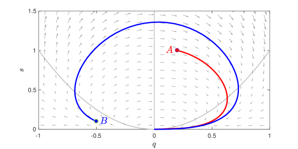
Figure 1. Illustration of the the phase plane of $(q,s)$ with $c=0$ and $N=2$. If the initial data $(q_{0},s_{0})=A$, the trajectory stays in $\mathbb{R}_{+}\times\mathbb{R}_{+}$, and converges to $(0,0)$. If the initial data $(q_{0},s_{0})=B$, the trajectory stays bounded, and will cross $q=0$ in finite time. Asymptotically, it also converges to $(0,0)$.

Lemma 3.3.

Consider the dynamics (26) with $q_{0}\geq 0$ and $s_{0}>0$, then $(q,s)$ remains bounded in all time. More precisely, there exists a constant $Q$ such that

$$q(t)\in[0,Q],\quad s(t)\in(0,s_{0}],\quad\forall~{}t\geq 0.$$

Moreover, $(q(t),s(t))$ converges to $(0,0)$ as $t\to\infty$.

Proof.

First, we show $q(t)\geq 0$ for all $t\geq 0$. Suppose the argument is false, then there exists a time $t_{0}$ such that $q(t_{0})=0$ and $q^{\prime}(t_{0})\leq 0$. On the other hand, $q^{\prime}(t_{0})=\kappa s(t_{0})>0$, which leads to a contradiction.

Then, by (27), we get $s(t)\leq s_{0}$. Therefore, $s$ is bounded.

Next, we claim that $q(t)\leq Q:=\max\{q_{0},\sqrt{\kappa s_{0}}\}$, using a similar argument by contradiction as the first part. Given any $\epsilon>0$, suppose there exists a $t_{0}$ such that $q(t_{0})=Q+\epsilon$, and $q(t_{0}+)>Q+\epsilon$. Then,

$$q^{\prime}(t_{0})=-(Q+\epsilon)^{2}+\kappa s(t_{0})\leq-Q^{2}-\epsilon(2Q+\epsilon)+\kappa s_{0}=-\epsilon(2Q+\epsilon)<0.$$

Therefore, $q(t_{0}+)<Q+\epsilon$, which leads to a contradiction. The proof is finished by taking $\epsilon\to 0$.

Finally, for the asymptotic behavior, we first observe that $s$ is bounded and decreasing and hence has a limit. Since the only steady state for $(q,s)\in[0,Q]\times[0,s_{0}]$ is $(0,0)$, $\lim_{t\to\infty}s(t)=0$. For $q$, let $t_{1}=\inf\{t\geq 0:s(t)<\frac{Q^{2}}{\kappa}\}$. Clearly, $t_{1}$ is finite. $q(t)$ is decreasing for $t\geq t_{1}$ and hence has a limit. Due to the only steady state $(0,0)$, the limit has to be $\lim_{t\to\infty}q(t)=0$. This concludes the proof. ∎

The more subtle case is when $q_{0}<0$, namely the initial velocity is pointing towards the origin. Without the term $\kappa s$, the dynamics $q^{\prime}=-q^{2}$ is known to blow up to $-\infty$ in finite time. The $\kappa s$ term could help avoid the blowup. The following theorem describes such phenomenon. Remarkably, when $n\geq 2$, the blowup won’t happen for any initial configuration, no matter how small $s_{0}$ is.

Theorem 3.4.

Let $n\geq 2$. Consider the dynamics (26) with initial data $q(0)<0$ and $s(0)>0$. Then, $(q,s)$ remains uniformly bounded in all time. Moreover, $(q(t),s(t))$ converges to $(0,0)$ as $t\to\infty$.

We first prove the theorem for dimension $n\geq 3$, or in general $n>2$ ($n$ does not to be an integer to make sense of the dynamics (26)).

Proof of Theorem 3.4 for $n\geq 3$.

First, we show that $q$ is bounded from below. Let us start with a rough estimate on $q$. Since $\kappa s>0$,

$$q^{\prime}\geq-q^{2}.$$

This implies $q(t)\geq\frac{q_{0}}{1+tq_{0}}$. Therefore, blowup can not happen before $T_{0}=-\frac{1}{q_{0}}$.

For any $t<T_{0}$ and $\tau<t$, we have

$$-\frac{1}{q(t)}+\frac{1}{q(\tau)}\geq-(t-\tau)\quad\Rightarrow\quad q(\tau)\leq\frac{q(t)}{1-q(t)(t-\tau)},\quad\forall~{}\tau\in[0,t).$$

Apply the estimate to (27), we obtain

$$s(t)\geq s_{0}\exp\left[-n\int_{0}^{t}\frac{q(t)}{1-q(t)(t-\tau)}d\tau\right]=s_{0}(1-tq(t))^{n}\geq s_{0}t^{n}(-q(t))^{n}.$$ (28)

Plug back in (26), we get an improve estimate on the dynamics of $q$

$$q^{\prime}(t)\geq-(-q(t))^{2}+\kappa s_{0}t^{n}(-q(t))^{n}.$$ (29)

Since $n>2$, the second term on the right hand side of (29) will dominate the first term, and $q^{\prime}(t)>0$ if $-q(t)$ is big enough. This avoids $q$ from becoming more negative, and hence prevents blowup.

In detail, for $t>T_{0}/2$,

$$q^{\prime}(t)>-(-q(t))^{2}+\frac{\kappa s_{0}T_{0}^{n}}{2^{n}}(-q(t))^{n}\geq 0,\quad\text{if}\quad-q(t)\geq\left(\frac{\kappa s_{0}T_{0}^{n}}{2^{n}}\right)^{-\frac{1}{n-2}}.$$

This implies

$$q(t)\geq\min\left\{q\left(\frac{T_{0}}{2}\right),-\left(\frac{\kappa s_{0}T_{0}^{n}}{2^{n}}\right)^{-\frac{1}{n-2}}\right\},\quad\forall~{}t>\frac{T_{0}}{2}.$$

Together with the rough estimate $q(t)\geq 2q(0)$ for all $t\leq T_{0}/2$, we end up with a uniform in time lower bound on $q$.

To get a uniform bound on $s$, we argue by contradiction. Suppose $s$ is not uniformly bounded. Since $s$ is bounded in all finite time, we must have $\lim_{t\to\infty}s(t)=\infty$. By Lemma 3.3, it must be true that $q(t)<0$ for all time, and hence $s(t)$ is increasing.

On the other hand, there exists a time $t_{0}$ such that $s(t_{0})>\kappa^{-1}(q_{\min}^{2}+1)$, where $q_{\min}$ denotes the lower bound of $q$. Then,

$$q^{\prime}(t)=-q(t)^{2}+\kappa s(t)\geq-q_{\min}^{2}+\kappa s(t_{0})>1,\quad\forall~{}t\geq t_{0}.$$

Consequently, we have $q(t)\geq q_{\min}+(t-t_{0})$, and then $q(t_{0}+(-q_{\min}))\geq 0$. This leads to a contradiction.

Therefore, there exists a finite time $t_{1}$ such that $s(t_{1})$ reaches the maximum, and $q(t_{1})=0$. Starting from $t_{1}$, we can apply Lemma 3.3 and get the upper bound on $q$ and the asymptotic behaviors. ∎

The two-dimensional case is critical, as the estimate (29) does not directly imply $q^{\prime}(t)>0$ for large $-q(t)$, if $s_{0}$ is small. To show boundedness of solutions for all $s_{0}>0$, we need to make further improvements to our estimates.

Proof of Theorem 3.4 for $n=2$.

We start with the same argument as $n>2$ case, which implies (28)

$$q^{\prime}(t)\geq\big{(}-1+s_{0}t^{2}\big{)}(-q(t))^{2}.$$ (30)

Then, $q(t)^{\prime}>0$ for any $t>s_{0}^{-1/2}$. Hence, blowup won’t happen after $T_{1}=s_{0}^{-1/2}$. Also, blowup can not happen before $T_{0}=-\frac{1}{q_{0}}$. Therefore, $q(t)$ is bounded from below in all time if $T_{0}>T_{1}$, or equivalently $s_{0}>(-q_{0})^{2}$. However, if $s_{0}$ is small $s_{0}\leq(-q_{0})^{2}$, then blowup can still occur at $t\in(T_{0},T_{1})$. In this scenario, we perform the following improved estimates.

For any $0\leq\tau<t<T_{0}$, from (30) we have

$$-\frac{1}{q(t)}+\frac{1}{q(\tau)}\geq-\left[t-\tau-\frac{s_{0}}{3}(t^{3}-\tau^{3})\right]~{}~{}\Rightarrow~{}~{}q(\tau)\leq\frac{q(t)}{1-q(t)\left[t-\tau-\frac{s_{0}}{3}(t^{3}-\tau^{3})\right]}.$$

This leads to an improved estimate on

$$\int_{0}^{t}q(\tau)d\tau\geq\int_{0}^{t}\frac{1}{\frac{1}{q(t)}-\tau+\frac{s_{0}}{3}(\tau^{2}-3t\tau+3t^{2})\tau}d\tau\geq\int_{0}^{t}\frac{1}{\frac{1}{q(t)}-\tau+\frac{s_{0}}{3}t^{2}\tau}d\tau$$

and then

$$s(t)\geq s_{0}\exp\left[-2\int_{0}^{t}\frac{1}{\frac{1}{q(t)}-(1-\frac{s_{0}}{3}t^{2})\tau}d\tau\right]=s_{0}\left[1-\left(1-\frac{s_{0}}{3}t^{2}\right)tq(t)\right]^{\frac{2}{1-\frac{s_{0}}{3}t^{2}}}.$$

Compared with the estimate (28) with $s(t)\gtrsim(-q(t))^{2}$, the improved estimate has $s(t)\gtrsim(-q(t))^{\alpha}$, with $\alpha=\frac{2}{1-\frac{s_{0}}{3}t^{2}}>2$. Now, we are able to finish the proof using the same argument as in the $n\geq 3$ case. Indeed, for $t>T_{0}/2$,

$$q^{\prime}(t)>-(-q(t))^{2}+\kappa s_{0}\left(1-\frac{s_{0}T_{0}^{2}}{12}\right)(-q(t))^{\frac{2}{1-\frac{s_{0}T_{0}^{2}}{12}}}\geq 0,$$

if $-q(t)$ is large enough,

$$-q(t)\geq\left[\kappa s_{0}\left(1-\frac{s_{0}T_{0}^{2}}{12}\right)\right]^{-\frac{12-s_{0}T_{0}^{2}}{2s_{0}T_{0}^{2}}}.$$

The uniform bound on $s$ and asymptotic behaviors can then be obtained the same as the $n>2$ case. ∎

Remark 3.5.

For $n<2$, the dynamics can lead to a finite time blowup if $q_{0}<0$ and $s_{0}$ is small enough. Therefore, $n\geq 2$ is a critical assumption for Theorem 3.4 to be valid. We skip the discussion for the $n<2$ case, as it is not relevant under our setup.

3.2.2. Asymptotic behavior

The next lemma shows the detailed asymptotic behavior of $(q,s)$ as time approaches infinity. The convergence rate will be useful for later discussions. Without loss of generality, we set $q_{0}\geq 0$. This is because we know that if $q_{0}<0$, there exists a finite time $t_{*}$ such that $q(t_{*})=0$. Same convergence rate can be obtained by a simple shift in time.

Lemma 3.6.

Consider the dynamics (26) with $q_{0}\geq 0$ and $s_{0}>0$. Then, there exist two positive constants $C_{q}$ and $\bar{C}_{s}$, depending on $n$ and $(q_{0},s_{0})$, such that

$$q(t)\leq C_{q}(t+1)^{-1},\quad s(t)\leq\bar{C}_{s}(t+1)^{-2},\quad\forall~{}t\geq 0.$$ (31)

Moreover, there exists a positive constant $C_{s}$, depending on $n$ and $(q_{0},s_{0})$, such that

$$s(t)\leq\begin{cases}C_{s}(t+1)^{-2}\left(\ln(t+1)+1\right)^{-1}&n=2\\ C_{s}(t+1)^{-n}&n\geq 3.\end{cases}.$$ (32)

Proof.

We apply the following transformation. Let

$$\hat{q}(t)=(t+1)q(t),\quad\hat{s}(t)=(t+1)^{2}s(t).$$

We can rewrite the dynamics (26) as

$$\begin{cases}\hat{q}^{\prime}=\frac{1}{t+1}\left(-\hat{q}^{2}+\hat{q}+\kappa\hat{s}\right),\\ \hat{s}^{\prime}=\frac{1}{t+1}(2-n\hat{q})\hat{s}.\end{cases}$$

and the pre-factor $\frac{1}{t+1}$ can be absorbed by changing the time variable to $\hat{t}=\ln(t+1)$. So, with respect to $\hat{t}$, the dynamics reads

$$\begin{cases}\hat{q}^{\prime}=\left(-\hat{q}^{2}+\hat{q}+\kappa\hat{s}\right),\\ \hat{s}^{\prime}=(2-n\hat{q})\hat{s}.\end{cases}$$ (33)

From a standard study of the autonomous system in the phase plane (see Figure 2), we know that for any $\hat{q}_{0}\geq 0,\hat{s}_{0}>0$, the dynamics converges to the steady state $(1,0)$. This implies $q(t)=O(t^{-1})$, and $s(t)=o(t^{-2})$. In particular, we can pick $C_{q}=\hat{q}_{\max}$.

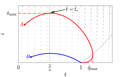
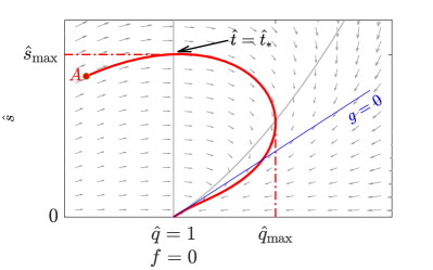
Figure 2. Illustration of the the phase plane of $(\hat{q},\hat{s})$. Left figure: $n\geq 3$, right figure $n=2$.

Now, we aim to obtain a better decay estimate on $s(t)$.

For $n\geq 3$. we observe from (33) and Figure 2 that $\hat{s}$ obtain its maximum value $\hat{s}_{\max}$ at a finite time $\hat{t}_{*}$ when $\hat{q}(\hat{t}_{*})=\frac{2}{n}$ (or $\hat{q}>\frac{2}{n}$ if $\hat{q}_{0}>\frac{2}{n}$, where $\hat{t}_{*}=0$). We can write

$$\hat{s}(\hat{t})=\hat{s}_{\max}\exp\left[\int_{\hat{t}_{*}}^{\hat{t}}\left(2-n\hat{q}(\hat{\tau})\right)\,d\hat{\tau}\right]=\hat{s}_{\max}\exp\left[(2-n)(\hat{t}-\hat{t}_{*})+n\int_{\hat{t}^{*}}^{\hat{t}}\left(1-\hat{q}(\hat{\tau})\right)\,d\hat{\tau}\right],$$ (34)

where we define $f(\hat{t})=q(\hat{t})-1$ which satisfies

$$f^{\prime}=-f^{2}-f+\kappa\hat{s}\geq-f^{2}+f,\quad f(t_{*})\geq\frac{2}{n}-1.$$

Explicit calculation yields

$$f(\hat{t})\geq-\frac{n-2}{n-2+2e^{\hat{t}-\hat{t}_{*}}}\geq-\frac{n-2}{2}e^{-(\hat{t}-\hat{t}_{*})},\quad\forall~{}\hat{t}\geq\hat{t}_{*}.$$

Therefore, the last integral in (34) is uniformly bounded

$$\int_{\hat{t}_{*}}^{\hat{t}}\left(1-\hat{q}(\hat{\tau})\right)\,d\hat{\tau}\leq\int_{0}^{\infty}\frac{n-2}{2}e^{-\hat{\tau}}\,d\hat{\tau}=\frac{n-2}{2}.$$

Finally, we obtain

$$s(t)=\hat{s}(\hat{t})(t+1)^{-2}\leq\hat{s}_{\max}e^{(n-2)\hat{t}_{*}+\frac{n(n-2)}{2}}(t+1)^{2-n}(t+1)^{-2}=:C_{s}(t+1)^{-n}.$$ (35)

We are left with the case $n=2$, which turns out to be critical. To obtain the logarithmic improvement in (31), we need to show $\hat{s}(\hat{t})\lesssim(\hat{t}+1)^{-1}$. Define two new variables

$$f=\hat{q}-1,\quad g=\kappa\hat{s}-\hat{q}+1.$$

Then, (33) can be equivalently expressed as

$$\begin{cases}f^{\prime}=-f^{2}+g,\\ g^{\prime}=(-1-2f)g-f^{2},\end{cases}\quad\text{with}\quad\begin{cases}f(\hat{t}_{*})=\hat{q}(\hat{t}_{*})-1\geq 0,\\ g(\hat{t}_{*})=\kappa\hat{s}(\hat{t}_{*})-f(\hat{t}_{*}).\end{cases}$$

Clearly, $f\geq 0$ is an invariant region. Then, we can easily find an upper bound of $g$ by

$$g(\hat{t})\leq\min\left\{g(\hat{t}_{*})e^{-(\hat{t}-\hat{t}_{*})},0\right\}.$$

Plugging back into the dynamics of $f$, we immediately obtain an upper bound of $f$

$$f(\hat{t})\leq C(\hat{t}-\hat{t}_{*}+1)^{-1},\quad\forall~{}\hat{t}\geq\hat{t}_{*},$$

where $C$ depends on $f(\hat{t}_{*})$ and $g(\hat{t}_{*})$. Finally, we conclude that

$$\hat{s}(\hat{t})=\frac{1}{\kappa}\big{(}f(\hat{t})+g(\hat{t})\big{)}\lesssim(\hat{t}+1)^{-1}.$$

∎

Remark 3.7.

In (31), the constant $C_{q}\geq 1$ as $\hat{q}_{\max}\geq 1$. Note that if $s_{0}$ is small enough, then $C_{q}$ is close to 1. In particular, as illustrated in the left figure in Figure 2, For the trajectory start at point $B$, $C_{q}=1$.

3.2.3. Explicit subcritical regions

We now switch to discuss the dynamics of $(p,\rho)$ in (24). Recall

$$\begin{cases}p^{\prime}=-p^{2}+\kappa(\rho-(n-1)s),\\ \rho^{\prime}=-\rho(p+(n-1)q).\end{cases}$$ (36)

Note that even if $(q,s)$ stays bounded uniformly in time, they affect the dynamics of $(p,\rho)$ when $n\geq 2$, and hence the subcritical region $\Sigma$ could be different than (25).

The goal here is to find a more explicit subcritical region. In particular, we need to make sure that the subcritical region is not an empty set in general.

To better understanding the dynamics of (46), we proceed with the following transformations. First, consider the dynamics of $(p/\rho,1/\rho)$

$$\begin{cases}\displaystyle\left(\frac{p}{\rho}\right)^{\prime}=\,\kappa+(n-1)\left(q\cdot\frac{p}{\rho}-\kappa s\cdot\frac{1}{\rho}\right),\\ \displaystyle\left(\frac{1}{\rho}\right)^{\prime}=\,\frac{p}{\rho}+(n-1)\frac{q}{\rho}.\end{cases}$$ (37)

To absorb the explicit dependence on $q$, we introduce new quantities $(w,v)$ along the characteristic paths as follows

$$w=\frac{p}{\rho}\cdot e^{(n-1)A(t)},\quad v=\frac{1}{\rho}\cdot e^{(n-1)A(t)},$$ (38)

where $A(t)$ is defined as

$$A(t):=-\int_{0}^{t}q(\tau)\,d\tau=\frac{1}{n}\ln\frac{s(t)}{s_{0}}.$$ (39)

The second equality directly comes from (27). As we have already know $s$ is uniformly bounded in time, so does $A$. Then, the dynamics of $(w,v)$ reads

$$\begin{cases}\displaystyle w^{\prime}=\,\kappa e^{(n-1)A}-\kappa\big{(}c+(n-1)s\big{)}v,\\ v^{\prime}=\,w.\end{cases}$$ (40)

Let us first summarize the threshold condition for $n=1$. In this case, (40) simply becomes

$$w^{\prime}=\kappa,\quad v^{\prime}=w.$$

Therefore, we obtain

$$w(t)=w_{0}+\kappa t,\quad\text{and}\quad v(t)=v_{0}+w_{0}t+\frac{\kappa}{2}t^{2}.$$

Then, $v(t)$ won’t reach zero if and only if $w_{0}>-\sqrt{2\kappa v_{0}}$. From the definition of $(w,v)$ (38), this is equivalent to $p_{0}>-\sqrt{2\kappa\rho_{0}}$.

When $n\geq 2$, we have $e^{(n-1)A}\not\equiv 1$ and $(n-1)sv\not\equiv 0$. The two terms reflect the contribution of $(q,s)$ to the dynamics of $(w,v)$. In particular, $e^{(n-1)A(t)}=\left(\frac{s(t)}{s_{0}}\right)^{\frac{n-1}{n}}$ vanishes as $t\to\infty$ due to Lemma 3.6. Therefore, the behavior of $(w,v)$ is different from the 1D case.

Let us state our result.

Theorem 3.8.

Let $n\geq 2$. There exists threshold function $\sigma_{+}~{}:~{}\mathbb{R}_{+}\to\mathbb{R}_{+}$, depending on $(q_{0},s_{0})$, such that

$$\left\{(p_{0},q_{0},s_{0},\rho_{0})~{}\left|~{}p_{0}>-\rho_{0}\sigma_{+}\left(\frac{1}{\rho_{0}};~{}q_{0},s_{0}\right)\right.\right\}\subset\Sigma.$$

Remark 3.9.

For $n=1$, $\sigma_{+}(x)=\sqrt{2\kappa x}$. For $n\geq 2$, we obtain a similar condition, allowing $p_{0}$ to be negative. $\sigma_{+}$ will depend on $(q_{0},s_{0})$, indicating the effect of the spectral gap.

Let us first consider the case $n\geq 3$. Write

$$w(t)=w_{0}+\kappa\int_{0}^{t}e^{(n-1)A(\tau)}\,d\tau-\kappa(n-1)\int_{0}^{t}s(\tau)v(\tau)\,d\tau.$$ (41)

Step 1: upper bounds on $w$ and $v$. Apply Lemma 3.6 and get

$$w(t)\leq \,w_{0}+\kappa s_{0}^{-\frac{n-1}{n}}\int_{0}^{t}s(\tau)^{\frac{n-1}{n}}\,d\tau\,\leq w_{0}+\kappa\left(\frac{C_{s}}{s_{0}}\right)^{\frac{n-1}{n}}\int_{0}^{t}(\tau+1)^{-(n-1)}\,d\tau$$

$$\leq \,w_{0}+\frac{\kappa}{n-2}\left(\frac{C_{s}}{s_{0}}\right)^{\frac{n-1}{n}}=:w_{0}+C(q_{0},s_{0}),$$

for $n\geq 3$. Therefore, unlike 1D where $w$ can grow linearly in time, $w$ is uniformly bounded. And $v$ can grow at most linearly

$$v(t)\leq v_{0}+\left(w_{0}+C(q_{0},s_{0})\right)t.$$ (42)

Remark 3.10.

If $w_{0}<-C(q_{0},s_{0})$, or equivalently $p_{0}<-C(q_{0},s_{0})\rho_{0}$, $v(t)$ will become negative in finite time. Hence, such initial data lie in the supercritical region.

Step 2: lower bounds on $w$ and $v$, assuming $w_{0}>-C(q_{0},s_{0})$. Let us control the two integrals in (41) one by one. For the first term, by (31) and (39), we have

$$A(t)\geq-\int_{0}^{t}C_{q}(\tau+1)^{-1}\,d\tau=-C_{q}\ln(t+1).$$

Then,

$$\kappa\int_{0}^{t}e^{(n-1)A(\tau)}\,d\tau\geq\kappa\int_{0}^{t}(\tau+1)^{-C_{q}(n-1)}\,d\tau=\frac{\kappa}{\gamma+1}\left(1-(t+1)^{-\gamma-1}\right),$$

where $\gamma=C_{q}(n-1)-2$. Note that from Remark 3.7, $C_{q}\geq 1$ (strict inequality for $n=3$) , we have $\gamma>0$ for $n\geq 3$.

For the second term, apply (31) and (42)

$$\int_{0}^{t}s(\tau)v(\tau)\,d\tau\leq \,\int_{0}^{t}C_{s}(\tau+1)^{-n}\big{(}v_{0}+\left(w_{0}+C(q_{0},s_{0})\right)\tau\big{)}\,d\tau$$

$$\leq \,C_{s}\left(\frac{v_{0}}{n-1}+\frac{w_{0}+C(q_{0},s_{0})}{n-2}\right).$$

Put the two estimates together, we have

$$w(t)\geq w_{0}-C_{s}\left(\frac{v_{0}}{n-1}+\frac{w_{0}+C(q_{0},s_{0})}{n-2}\right)+\frac{\kappa}{\gamma+1}\left(1-(t+1)^{-\gamma-1}\right).$$

Denote

$$D:=-w_{0}+C_{s}\left(\frac{v_{0}}{n-1}+\frac{w_{0}+C(q_{0},s_{0})}{n-2}\right).$$

Then, we get

$$w(t)\geq \,-D+\frac{\kappa}{\gamma+1}\left(1-(t+1)^{-\gamma-1}\right),$$

$$v(t)\geq \,v_{0}+\left(-D+\frac{\kappa}{\gamma+1}\right)t-\frac{\kappa}{\gamma(\gamma+1)}\left(1-(t+1)^{-\gamma}\right).$$

To complete the lower bound estimate, we state the following lemma.

Lemma 3.11.

Let $y(t)$ be a function defined as

$$y(t)=v_{0}+\left(\frac{\kappa}{\gamma+1}-D\right)t-\frac{\kappa}{\gamma(\gamma+1)}\left(1-(t+1)^{-\gamma}\right).$$

Then, there exists a constant $D_{crit}=D_{crit}(v_{0})>0$, depending on initial data $v_{0}$, and parameters $\gamma,\kappa$, such that if $D<D_{crit}$, then $y(t)>0$ for all $t\in[0,\infty)$.

Proof.

For $D\leq 0$, the result is trivial as $y(t)\geq v_{0}>0$. On the other hand, if $D>\frac{\kappa}{\gamma+1}$, $y(t)\leq v_{0}-\left(D-\frac{\kappa}{\gamma+1}\right)t$ will reach zero in finite time, regardless of the choice of $v_{0}$. Hence, $D_{crit}\leq\frac{\kappa}{\gamma+1}$.

Let us focus on $D\in(0,\frac{\kappa}{\gamma+1}]$. For simplified notations, let $z=1-\frac{\gamma+1}{\kappa}D\in[0,1)$. The minimum of $y$ is attained at $t_{*}=z^{-\frac{1}{\gamma+1}}-1$. We calculate

$$y_{\min}=y(t_{*})= \,v_{0}+\frac{\kappa}{\gamma+1}z^{\frac{\gamma}{\gamma+1}}-\frac{\kappa}{\gamma+1}z-\frac{\kappa}{\gamma(\gamma+1)}\left(1-z^{\frac{\gamma}{\gamma+1}}\right)$$

$$= \,v_{0}+\frac{\kappa}{\gamma}z^{\frac{\gamma}{\gamma+1}}-\frac{\kappa}{\gamma+1}\left(z+\frac{1}{\gamma}\right)=:F(z).$$

We can view the minimum as a function of $z$. Observe that $F$ is an increasing function in $[0,1]$, $F(1)=v_{0}>0$, and $F(0)=v_{0}-\frac{\kappa}{\gamma(\gamma+1)}$. Therefore, we have

• If $v_{0}<\frac{\kappa}{\gamma(\gamma+1)}$, $F$ has a unique root $z_{*}\in(0,1)$, and $F(z)>0$ for all $z>z_{*}$. Therefore, if $D<D_{crit}:=\frac{\kappa}{\gamma+1}(1-z_{*})$, then $y_{\min}>0$.

• If $v_{0}\geq\frac{\kappa}{\gamma(\gamma+1)}$, $F(z)>0$ for all $z\in(0,1)$. Hence, if $D<D_{crit}:=\frac{\kappa}{\gamma+1}$, $y_{\min}>0$.

∎

Step 3: conclusion. As a direct consequence of Lemma 3.11, we obtain a subcritical condition $D<D_{crit}$, which can be conveniently rewritten as

$$w_{0}>\left[-D_{crit}(v_{0})+C_{s}\left(\frac{v_{0}}{n-1}+\frac{C(q_{0},s_{0})}{n-2}\right)\right]\left(1-\frac{C_{s}}{n-2}\right)^{-1}=:-\sigma_{+}(v_{0}).$$ (43)

This finishes the proof of Theorem 3.8.

Remark 3.12.

The constant $C_{s}$ can be small so that the right hand side of (43) is negative. Indeed, in the case when $q_{0}>\frac{2}{n}$, we have $\hat{s}_{\max}=s_{0}$ and $\hat{t}_{*}=0$ in (35). Then, $C_{s}=s_{0}e^{\frac{n(n-2)}{2}}$ is small as long as $s_{0}$ is small. For general case, particularly $q_{0}<0$, a similar argument works for the dynamics starting at time $t=t_{*}$. Since $t_{*}$ is finite, it is easy to control $v(t)$ for $t<t_{*}$. We omit the technical details here for simplicity.

For $n=2$, due to its criticality, the calculation would be slightly different. Thanks to the logarithmic improvement in (32), we are able to obtain a similar result. We shall only sketch the proof, highlighting the difference.

First, $w(t)$ is not bounded by a constant, but could have a logarithmic growth.

$$w(t)\leq ~{}w_{0}+2\kappa\left(\frac{C_{s}}{s_{0}}\right)^{\frac{1}{2}}\Big{(}\ln(t+1)+1\Big{)}^{\frac{1}{2}},$$

$$v(t)\leq ~{}v_{0}+w_{0}t+2\kappa\left(\frac{C_{s}}{s_{0}}\right)^{\frac{1}{2}}t\Big{(}\ln(t+1)+1\Big{)}^{\frac{1}{2}}.$$

Next, for the lower bound, since the estimates above do not imply boundedness of $\int_{0}^{t}s(\tau)v(\tau)\,d\tau$, the previous estimates for $n\geq 3$ does not follow. Instead, we write

$$w^{\prime}=\kappa\left(\frac{s}{s_{0}}\right)^{\frac{1}{2}}-\kappa sv=\kappa s^{\frac{1}{2}}\left(s_{0}^{-\frac{1}{2}}-s^{\frac{1}{2}}v\right),$$

and the term $s^{\frac{1}{2}}v$ is bounded and

$$s^{\frac{1}{2}}v\leq ~{}C_{s}^{\frac{1}{2}}(t+1)^{-1}\Big{(}\ln(t+1)+1\Big{)}^{-\frac{1}{2}}\left(v_{0}+w_{0}t+2\kappa\left(\frac{C_{s}}{s_{0}}\right)^{\frac{1}{2}}t\Big{(}\ln(t+1)+1\Big{)}^{\frac{1}{2}}\right)$$

$$\rightarrow ~{}2\kappa C_{s}s_{0}^{-\frac{1}{2}},\quad\text{as}\quad t\to+\infty.$$

Therefore, if we choose a small $C_{s}$ such that $2\kappa C_{s}<1$, then $w^{\prime}$ will eventually become positive. One can continue with a similar argument as in the $n\geq 3$ case to obtain a threshold condition in Theorem 3.8. The technical details will be omitted.

3.3. Multi-dimensional case with positive constant background

Now, we study the Euler-Poisson equations with constant background $c>0$. It is known that the behavior of the solution is very different from the zero background case. We will start with analyzing the $(q,s)$ pair in the phase plane.

3.3.1. Uniform boundedness of $(q,s)$

Recall the $(q,s)$ dynamics for the case $c>0$

$$\begin{cases}q^{\prime}=-q^{2}+\kappa s,\\ s^{\prime}=-(ns+c)q.\end{cases}$$ (44)

Compared with the zero background case, the main difference is that, since $s$ can be negative, $q(t)\geq 0$ is no longer an invariant region. So Lemma 3.3 does not apply. In the phase plane of $(q,s)$, The steady state $(0,0)$ is not an attractor. As illustrated in Figure 3, the trajectories of $(q,s)$, if bounded, form periodic orbits, and do not converge as the time approaches infinity.

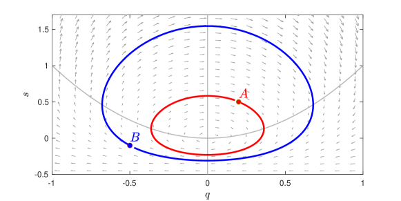
Figure 3. Illustration of the the phase plane of $(q,s)$ with $c=1$ and $N=2$. For any initial data (both $A$ and $B$ as examples), the solution are bounded uniformly in time. The trajectories form close orbits around $(0,0)$ that are symmetric in $s$-axis. The solutions are periodic in time.

Theorem 3.13 (Boundedness of $(q,s)$).

Let $n\geq 2$. Consider the $(q,s)$ dynamics in (44) with bounded initial conditions $(q_{0},s_{0})$ such that $s_{0}>-\frac{c}{n}$. Then, $(q(t),s(t))$ remains bounded in all time. Moreover, the trajectory of $(q(t),s(t))$ stays on a bounded periodic orbit in the $(q,s)$-plane.

Proof.

Let us perform the following convenient transformation

$$\tilde{s}=s+\frac{c}{n}.$$

The dynamics of $(q,\tilde{s})$ reads

$$\begin{cases}q^{\prime}=-q^{2}+\kappa\tilde{s}-\frac{\kappa c}{n},\\ \tilde{s}^{\prime}=-n\tilde{s}q,\end{cases}$$ (45)

and we are only interested in the case when $\tilde{s}_{0}>0$, which clearly preserves in time.

We first express $\tilde{s}$ in terms of $q$ as

$$\tilde{s}(t)=\tilde{s}_{0}\exp\left[-n\int_{0}^{t}q(\tau)d\tau\right].$$

Immediately, we obtain a lower bound $\tilde{s}(t)>0$ as long as $q$ stays bounded.

Assume by contradiction, there exist a first time $T_{*}$ such that solution becomes unbounded. $T_{*}$ can be either finite (corresponding to finite time blowup), or infinity. Then, at least one of the three scenarios happen:

$$\lim_{t\to T_{*}-}q(t)=+\infty,\quad\lim_{t\to T_{*}-}q(t)=-\infty,\quad\text{or}\quad\lim_{t\to T_{*}-}\tilde{s}(t)=+\infty.$$

We will show all three scenarios leads to contradictions.

First, if $\lim_{t\to T_{*}-}q(t)=+\infty$, there must exists time $t_{0}\in[0,T_{*})$ such that $q(t)>0$ for every $t\in[t_{0},T_{*})$. Then, $\tilde{s}^{\prime}(t)<0$ and hence $\tilde{s}(t)\leq\tilde{s}(t_{0})$ for every $t\in[t_{0},T_{*})$. On the other hand, from the dynamics of $q$, we have

$$q^{\prime}(t)\leq-q^{2}(t)+\kappa\tilde{s}(t_{0})<0,\quad\text{if}\quad q(t)\geq\sqrt{\kappa\tilde{s}(t_{0})},\quad\forall~{}t\in[t_{0},T_{*}).$$

This implies that $q(t)\leq\max\{q(t_{0}),\,\sqrt{\kappa\tilde{s}(t_{0})}\}$, which leads to a contradiction.

Second, if $\lim_{t\to T_{*}-}q(t)=-\infty$, there must exists a time $t_{0}\in[0,T_{*})$ such that $q(t)<-\sqrt{\frac{\kappa c}{n}}$ for every $t\in[t_{0},T_{*})$. A rough estimate on $q$ would read

$$q^{\prime}\geq-q^{2}-\frac{\kappa c}{n}\geq-2q^{2},\quad\forall t\in[t_{0},T_{*}),$$

The rest of the proof will be identical to Theorem 3.4, with only changes on the constant coefficients, as well as a shift of time variable by $t_{0}$. The result shows that $q(t)$ has a lower bound in all time, which clearly leads to a contradiction.

Third, $\lim_{t\to T_{*}-}\tilde{s}(t)=+\infty$, there must exists a time $t_{0}\in[0,T_{*})$ such that $\tilde{s}(t)>\kappa^{-1}(Q^{2}+\frac{\kappa c}{n}+1)$ for every $t\in[t_{0},T_{*})$, where $Q=\sup_{t\in[0,T_{*})}|q(t)|$ which is finite. Then,

$$q^{\prime}(t)=-q(t)^{2}+\kappa\tilde{s}(t)-\frac{\kappa c}{n}\geq-Q^{2}+\kappa\tilde{s}(t)-\frac{\kappa c}{n}>1,\quad\forall~{}t\in[t_{o},T_{*}).$$

Then, $q$ has a better lower bound

$$q(t)\geq-Q+(t-t_{0})\geq\begin{cases}-Q&t_{0}\leq t<t_{0}+Q\\ 0&t>t_{0}+Q\end{cases}$$

and therefore

$$\tilde{s}(t)=\tilde{s}(t_{0})\exp\left[-n\int_{t_{0}}^{t}q(\tau)d\tau\right]\leq\tilde{s}(t_{0})e^{nQ^{2}},\quad\forall~{}t\in[t_{0},T_{*}).$$

This leads to a contradiction.

Finally, the trajectory of the dynamics is symmetric in $q$ (by simple observations from (45)). Therefore, the solution is periodic in time, and travels along a closed orbit in the $(q,\tilde{s})$-phase plane. ∎

3.3.2. Subcritical regions

The dynamics of $(p,\rho)$ in (24) reads

$$\begin{cases}p^{\prime}=-p^{2}+\kappa(\rho-c-(n-1)s),\\ \rho^{\prime}=-\rho(p+(n-1)q).\end{cases}$$ (46)

We introduce the same variables $(w,v)$ in (38), with $A(t)$ defined as

$$A(t):=-\int_{0}^{t}q(\tau)\,d\tau=\frac{1}{n}\ln\frac{\tilde{s}(t)}{\tilde{s}_{0}}.$$

The dynamics of $(w,v)$ has the form

$$\begin{cases}\displaystyle w^{\prime}=\,\kappa e^{(n-1)A}-\kappa\big{(}c+(n-1)s\big{)}v,\\ v^{\prime}=\,w.\end{cases}$$ (47)

If $n=1$, the dynamics (47) is simply a closed linear system

$$w^{\prime}=\kappa(1-cv),\quad v^{\prime}=w,$$ (48)

which can be solved explicitly. The trajectory of the solution $(w,v)$ in the phase plane form a ellipse

$$\frac{w^{2}}{c\kappa}+\left(v-\frac{1}{c}\right)^{2}=R^{2},$$

where $R$ is determined by the initial condition $(w_{0},v_{0})$. $v(t)>0$ is then equivalent to $R<\frac{1}{c}$, or $w_{0}^{2}<\kappa(2v_{0}-cv_{0}^{2})$. This leads to the sharp threshold condition in (25).

However, with the effect of the spectral gap, it is very difficult to extend the 1D result in the multiple dimensions. Unlike the zero background case where the solution intends to converge to the equilibrium, the comparison principle fails as the solution oscillates. Moreover, the period for $(q,s)$ does not necessarily match with the period in (48), leading to a more chaotic dynamics. Hence, an explicit expression of the subcritical regions, like Theorem 3.8, remains to be a challenging open problem.

4. Application to the Euler-alignment equations

In this section, we discuss the Euler-alignment equations

$$\partial_{t}\rho+\nabla\cdot(\rho\mathbf{u})=0,$$

$$\partial_{t}\mathbf{u}+(\mathbf{u}\cdot\nabla)\mathbf{u}=\int_{\mathbb{R}^{n}}\phi(|\mathbf{x}-\mathbf{y}|)(\mathbf{u}(\mathbf{y})-\mathbf{u}(\mathbf{x}))\rho(\mathbf{y})d\mathbf{y}.$$

The system arises as the macroscopic representation of the Cucker-Smale flocking dynamics, describing the emergent phenomenon of animal flocks.

The nonlocal alignment force is modeled through an influence function $\phi$. Here, we assume $\phi$ is bounded, Lipschitz, non-increasing, and decays slowly at infinity

$$\int^{\infty}\phi(r)\,dr=\infty.$$ (49)

We state the local wellposedness theorem for the Euler-alignment equations, the same as Theorem 3.1. The proof can be found in, for instance, [18, 20].

Theorem 4.1 (Local wellposedness).

Consider the Euler-alignment equations with initial data $\rho_{0}\in H^{s}(\mathbb{R}^{n})$ and $\mathbf{u}_{0}\in H^{s+1}(\mathbb{R}^{n})^{n}$, for $s>\frac{n}{2}$. Then, there exists a time $T>0$ such that the solution

$$(\rho,\mathbf{u})\in C([0,T],H^{s}(\mathbb{R}^{n}))\times C([0,T],H^{s+1}(\mathbb{R}^{n}))^{n}.$$ (50)

Moreover, the life span $T$ can be extended as long as

$$\int_{0}^{T}\|\nabla\mathbf{u}(\cdot,t)\|_{L^{\infty}}\,dt<+\infty.$$ (51)

The slow-decay condition (49) is known to ensure the asymptotic flocking behavior.

Theorem 4.2 (Strong solution must flock [18]).

Let $(\rho,\mathbf{u})$ be a strong solution of the Euler-alignment system, with compactly supported initial density $\rho_{0}$, and the influence function satisfies $\phi$ the condition (49). Then, the solution must flock, namely, there exists a constant $D$, depending on the initial data, such that

$$\text{supp}(\rho(\cdot,t))\subset B_{D}(0),\quad\forall~{}t\geq 0,$$ (52)

where $B_{D}(0)$ is the ball in $\mathbb{R}^{n}$ that is centered at origin with radius $D$. Moreover, the solution exhibits fast alignment,

$$V(t)\leq V_{0}~{}e^{-\nu t},\quad V(t):=\sup_{x,y}|u(x,t)-u(y,t)|.$$ (53)

with an exponential rate of decay

$$\nu=\phi(2D)\|\rho_{0}\|_{L^{1}}>0.$$ (54)

In the following, we focus on the radially symmetric setup (11). The starting point is to verify that the force $\mathbf{F}$ has the form (12), so radial symmetry preserves in time. Express the nonlocal alignment force as

$$\mathbf{F}=\int_{\mathbb{R}^{n}}\phi(|\mathbf{x}-\mathbf{y}|)(\mathbf{u}(\mathbf{y},t)-\mathbf{u}(\mathbf{x},t))\rho(\mathbf{y},t)d\mathbf{y}=\mathcal{L}(\rho\mathbf{u})-\mathbf{u}\mathcal{L}\rho,$$

where

$$\mathcal{L}f(\mathbf{x}):=\int_{\mathbb{R}^{n}}\phi(|\mathbf{x}-\mathbf{y}|)f(\mathbf{y})d\mathbf{y}.$$

Under radial symmetry (11), it is easy to check that $\mathcal{L}\rho$ is a radial function, as the convolution of radial functions are radial. Let us denote

$$\psi(r)=\mathcal{L}\rho.$$ (55)

The term $\mathcal{L}(\rho\mathbf{u})$ can be expressed as follows.

Proposition 4.3.

The vector-valued function $\mathcal{L}(\rho\mathbf{u})$ can be written as

$$\frac{\mathbf{x}}{r}\zeta(r)=\mathcal{L}(\rho\mathbf{u}),$$

where $\zeta$ is defined as

$$\zeta(r)=\int_{\mathbb{R}^{n}}\phi(|r\mathbf{e}_{1}-\mathbf{z}|)\rho(|\mathbf{z}|)\frac{z_{1}}{|\mathbf{z}|}u(|\mathbf{z}|)d\mathbf{z},$$ (56)

with $\mathbf{e}_{1}=[1,0,\cdots,0]^{T}$.

Proof.

Let $U$ be a unitary matrix in $\mathbb{R}^{n}$ such that its first column is $\mathbf{x}/r$, namely

$$\mathbf{x}=rU{\bf e}_{1}.$$

Since the length $|\cdot|$ is invariant under unitary transformation, we have

$$|\mathbf{x}-\mathbf{y}|=|U^{T}(\mathbf{x}-\mathbf{y})|=|r\mathbf{e}_{1}-U^{T}y|.$$

Then, we can compute

$$\mathcal{L}(\rho\mathbf{u})= ~{}\int_{\mathbb{R}^{n}}\phi(|r\mathbf{e}_{1}-U^{T}\mathbf{y}|)\rho(|\mathbf{y}|)\frac{\mathbf{y}}{|\mathbf{y}|}u(|\mathbf{y}|)d\mathbf{y}=\int_{\mathbb{R}^{n}}\phi(|r\mathbf{e}_{1}-\mathbf{z}|)\rho(|\mathbf{z}|)\frac{U\mathbf{z}}{|\mathbf{z}|}u(|\mathbf{z}|)d\mathbf{z}$$

$$= ~{}\sum_{k=1}^{n}U\mathbf{e}_{k}\int_{\mathbb{R}^{n}}\phi(|r\mathbf{e}_{1}-\mathbf{z}|)\rho(|\mathbf{z}|)\frac{z_{k}}{|\mathbf{z}|}u(|\mathbf{z}|)d\mathbf{z}$$

$$= ~{}\frac{\mathbf{x}}{r}\int_{\mathbb{R}^{n}}\phi(|r\mathbf{e}_{1}-\mathbf{z}|)\rho(|\mathbf{z}|)\frac{z_{1}}{|\mathbf{z}|}u(|\mathbf{z}|)d\mathbf{z}.$$

For the last equality, we use the fact that for $k\geq 2$, the function is odd with respect to $z_{k}$, and hence the integral is zero. ∎

Combining Proposition 4.3 and (55), we have verified (12) with $F=\zeta-\psi u$. The dynamics of the radial profile $(\rho,u)$ reads

$$\begin{cases}\rho_{t}+(\rho u)_{r}=-\displaystyle(n-1)\frac{\rho u}{r},\\ u_{t}+uu_{r}=\zeta-\psi u.\end{cases}$$

Let us write out the dynamics of the pair $(p,q)$ in (15) as follows

$$\begin{cases}p^{\prime}=-p^{2}+\zeta_{r}-p\psi-u\psi_{r},\\ q^{\prime}=-q^{2}+\displaystyle\frac{\zeta}{r}-q\psi,\end{cases}$$

where again ${}^{\prime}=\partial_{t}+u\partial_{r}$ denotes the material derivative.

To eliminate the nonlocal term $\zeta_{r}$, we follow the idea introduced in [1]. Calculate the dynamics of $\psi$

$$\psi_{t}=\partial_{t}\mathcal{L}\rho=-\nabla\cdot\mathcal{L}(\rho\mathbf{u})=-\zeta_{r}-(n-1)\frac{\zeta}{r}.$$

Then, adding the dynamics of $p$ and $\psi$ would yield

$$(p+\psi)^{\prime}=-p(p+\psi)-(n-1)\frac{\zeta}{r}.$$ (57)

Let $G=p+\psi$. We summarize the dynamics on $(\rho,G)$

$$\begin{cases}\rho_{t}+(\rho u)_{r}=-(n-1)\rho q,\\ G_{t}+(Gu)_{r}=-(n-1)\displaystyle\frac{\zeta}{r}.\end{cases}$$ (58)

4.1. The one-dimensional case

When $n=1$, the right hand side of (58) vanishes. In particular, $G$ satisfies the continuity equation $G_{t}+(Gu)_{r}=0$. Therefore, $G\geq 0$ is an invariant region. Further investigation leads to a sharp threshold condition.

Theorem 4.4 (1D sharp threshold [1]).

Consider the Euler-alignment system in 1D.

• (Subcritical region) If $\inf G_{0}\geq 0$, the solution is globally regular.

• (Supercritical region) If $\inf G_{0}<0$, there exists a finite time blowup.

4.2. The effect of the spectral gap

When $n\geq 2$, extra terms appear in (58) involving $q$ and $\zeta/r$, which can not be locally expressed in terms of $(\rho,G)$ along a characteristic path. These two quantities encode the main difference between 1D and multi-dimensions, and hence is related to the spectral gap effect.

Let us first focus on $\zeta/r$.

One way to eliminate the term $\zeta/r$ is to take a linear combination of $G=p+\psi$ and $q$ as follows

$$(d+\psi)^{\prime}=(p+\psi+(n-1)q)^{\prime}=-p(p+\psi)-(n-1)q(q+\psi),$$

where $d=\nabla\cdot\mathbf{u}$. However, this does not reduce the problem to the one-dimensional case, as the right hand side of the dynamics is different from $-d(d+\psi)$. One needs to control the spectral gap $\eta$ in (7), which could be difficult. This approach has been investigated in [9] only for $n=2$.

As we have argued throughout the paper, we shall study the pair $(p,q)$ instead of $d$. To this end, we obtain a bound on $\zeta/r$.

Proposition 4.5 (Boundedness of $\zeta/r$).

The quantity $\frac{\zeta(r,t)}{r}$ is uniformly bounded in $(r,t)\in\mathbb{R}_{+}\times\mathbb{R}_{+}$. Moreover, it decays exponentially in time, with the same rate as in (53), thus, there exists a constant $C_{0}$, depending on the initial data, such that

$$\sup_{r>0}\frac{|\zeta(r,t)|}{r}\leq B(t):=C_{0}e^{-\nu t}.$$ (59)

Proof.

We estimate $\zeta$ from its definition (56).

$$|\zeta(r,t)|= \,\left|\int_{\mathbb{R}^{n}}(\phi(|r\mathbf{e}_{1}-\mathbf{z}|)-\phi(|\mathbf{z}|))\rho(|\mathbf{z}|,t)\frac{z_{1}}{|\mathbf{z}|}u(|\mathbf{z}|,t)\,d\mathbf{z}\right|$$

$$\leq \,\int_{\mathbb{R}^{n}}\|\phi^{\prime}\|_{L^{\infty}}|r\mathbf{e}_{1}|\rho(|\mathbf{z}|,t)\left|\frac{z_{1}}{|\mathbf{z}|}\right|u(|\mathbf{z}|,t)\,d\mathbf{z}$$

$$\leq \,r\|\phi^{\prime}\|_{L^{\infty}}\|\rho(\cdot,t)\|_{L^{1}}\|u(\cdot,t)\|_{L^{\infty}}\leq r\|\phi^{\prime}\|_{L^{\infty}}\|\rho_{0}\|_{L^{1}}\|u_{0}\|_{L^{\infty}}e^{-\nu t}.$$

For the first equality, odd symmetry in $z_{1}$ is used. For the last inequality, the fast alignment estimate (53) is applied. Note that due to the symmetry on $\mathbf{u}$, it is easy to check that $V(t)=2\|u(\cdot,t)\|_{L^{\infty}}$.

This ends the proof of (59), with $C_{0}=\|\phi^{\prime}\|_{L^{\infty}}\|\rho_{0}\|_{L^{1}}\|u_{0}\|_{L^{\infty}}$. ∎

Remark 4.6.

While $\zeta/r$ is bounded and decay in time, it does not necessarily has a definite sign. Therefore, $G\geq 0$ is no longer an invariant region, and we do not expect that the sharp threshold result in 1D (Theorem 4.4) remains true in multi-dimensions.

Next, we work on $q$. Recall its dynamics

$$q^{\prime}=-q^{2}+\frac{\zeta}{r}-q\psi.$$ (60)

We have obtained the boundedness of $\zeta/r$ in Proposition 4.5. The boundedness of $\psi$ can also be derived as follows.

Proposition 4.7 (Boundedness of $\psi$).

$\psi$ is bounded above and below by

$$0<\nu\leq\psi(r,t)\leq{\psi_{M}},\quad\forall~{}(r,t)\in[0,D]\times\mathbb{R}_{+}.$$

where $\nu$ is defined in (54), and ${\psi_{M}}:=\|\phi\|_{L^{\infty}}\|\rho_{0}\|_{L^{1}}$.

Proof.

The upper bound can be simply obtained by

$$\psi(r,t)=\int_{\mathbb{R}^{n}}\phi(r\mathbf{e}_{1}-y)\rho(y,t)\,dy\leq\|\phi\|_{L^{\infty}}\|\rho_{0}\|_{L^{1}}=:{\psi_{M}}.$$

For the lower bound, using the a priori bound on the support (52), the decreasing property of $\phi$, and the definition of $\nu$ in (54), we get

$$\psi(r,t)=\int_{|y|\leq D}\phi(r\mathbf{e}_{1}-y)\rho(y,t)\,dy\geq\phi(2D)\int_{|y|\leq D}\rho(y,t)\,dy=\nu.$$

∎

Now, we are ready to discuss threshold conditions on $q$. First, we state a rough result, making use of the boundedness on $\zeta/r$ and $\psi$.

Proposition 4.8 (Rough threshold conditions on $q$).

• (Subcritical region) Let $C_{0}\leq\frac{\nu^{2}}{4}$. If $q_{0}\geq\frac{1}{2}\left(-\nu-\sqrt{\nu^{2}-4C_{0}}\right)$, then $q(t)$ stays bounded in all time.

• (Supercritical region) If $q_{0}<\frac{1}{2}\left(-{\psi_{M}}-\sqrt{{\psi_{M}}^{2}+4C_{0}}\right)$, then $q(t)\to-\infty$ in finite time.

Proof.

The results follows from simple comparison principles. We will only show the subcritical region.

The upper bound on $q$ is trivial. If $q(t)\geq\sqrt{C_{0}}$, then

$$q^{\prime}(t)\leq-q^{2}(t)+C_{0}-\nu~{}q(t)<0.$$

This directly implies $q(t)\leq\max\{q_{0},\sqrt{C_{0}}\}$.

For the lower bound, we will show that $q(t)\geq\frac{1}{2}\left(-\nu-\sqrt{\nu^{2}-4C_{0}}\right)$, by contradiction. Suppose $q$ does not have such lower bound. Then, there exists a time $t_{0}$ such that $q(t_{0})=\frac{1}{2}\left(-\nu-\sqrt{\nu^{2}-4C_{0}}\right)$ and $q^{\prime}(t_{0})\leq 0$. On the other hand, we compute

$$q^{\prime}(t_{0})>-q^{2}(t_{0})-C_{0}-\nu~{}q(t_{0})=0.$$

This leads to a contradiction. ∎

The thresholds conditions are not sharp, due to the lack of precise control of the non-locality. However, in the special case when $\phi$ is a constant, we have $\zeta=0$ and $\nu={\psi_{M}}$. Then, Proposition 4.8 becomes sharp.

The threshold conditions can be improved, if we take into account of the fast decay property of $\zeta/r$. The idea is to the dynamics as the following autonomous system

$$\begin{cases}q^{\prime}=-q^{2}-c_{1}q+c_{2}B,\quad c_{1}\in[\nu,{\psi_{M}}],~{}~{}c_{2}\in[-1,1],\\ \frac{d}{dt}B=-\nu B,\end{cases}\quad\begin{cases}q(0)=q_{0},\\ B(0)=C_{0}.\end{cases}$$ (61)

Then, perform a phase plane analysis on (61) assuming $c_{1}$ and $c_{2}$ are constant. Finally, establish a comparison principle to obtain threshold conditions for (61). Following directly from [18, Theorem 5.1], we have the following enhanced threshold conditions.

Proposition 4.9 (Enhanced threshold conditions on $q$).

• (Subcritical region) There exists a function $\sigma_{q}^{+}:\mathbb{R}_{+}\to[-\nu,\infty)$, defined as

  $$\sigma_{q}^{+}(0)=-\nu,\quad\frac{d}{dx}\sigma_{q}^{+}(x)=\begin{cases}\displaystyle\frac{1}{2\nu},&x\to 0+\\ \displaystyle\frac{-\sigma_{q}^{+}(x)^{2}-\nu\sigma_{q}^{+}(x)-x}{-\nu x}&\text{if}~{}\sigma_{q}^{+}(x)<0\\ \displaystyle\frac{-\sigma_{q}^{+}(x)^{2}-{\psi_{M}}\sigma_{q}^{+}(x)-x}{-\nu x}&\text{if}~{}\sigma_{q}^{+}(x)\geq 0\end{cases}$$ (62)

  such that, if $q_{0}\geq\sigma_{q}^{+}(C_{0})$, then $q(t)$ stays bounded in all time.

• (Supercritical region) There exists a function $\sigma_{q}^{+}:\mathbb{R}_{+}\to[-\infty,-{\psi_{M}})$, defined as

  $$\sigma_{q}^{-}(0)=-{\psi_{M}},\quad\frac{d}{dx}\sigma_{q}^{-}(x)=\begin{cases}\displaystyle-\frac{1}{{\psi_{M}}+\nu},&x\to 0+\\ \displaystyle\frac{-\sigma_{q}^{-}(x)^{2}-{\psi_{M}}\sigma_{q}^{-}(x)+x}{-\nu x}&x>0.\end{cases}$$ (63)

  such that, if $q_{0}<\sigma_{q}^{-}(C_{0})$, then $q(t)\to-\infty$ in finite time.

Remark 4.10.

The threshold functions $\sigma_{q+}$ and $\sigma_{q-}$ only depends on $\nu$ and ${\psi_{M}}$. Figure 4 shows an example of the thresholds, with $\nu=.8$ and ${\psi_{M}}=1$. One can clearly see that the enhanced threshold conditions are much stronger than the rough conditions in Proposition 4.8, particularly for the subcritical region.

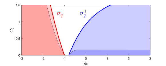
Figure 4. An illustration of the threshold regions for $(q_{0},C_{0})$ with parameters $\nu=.8,{\psi_{M}}=1$. Darker areas represent the rough conditions.

4.3. Critical thresholds in multi-dimensions

We are ready to control $\rho$ and $G$. In 1D, $G_{0}\geq 0$ is the sufficient and necessary condition to insure global regularity. It is not the case in multi-dimension, due to the effect of the spectral gap. Recall the dynamics of $G$

$$G^{\prime}=-G^{2}+\psi G-(n-1)\frac{\zeta}{r}.$$

A similar argument as Proposition 4.8 would yield the following rough conditions.

Proposition 4.11 (Rough threshold conditions on $G$).

• (Subcritical region) Let $C_{0}\leq\frac{\nu^{2}}{4(n-1)}$. If $G_{0}\geq\frac{1}{2}\left(\nu-\sqrt{\nu^{2}-4(n-1)C_{0}}\right)$, then $G(t)$ stays bounded in all time.

• (Supercritical region) If $G_{0}<\frac{1}{2}\left({\psi_{M}}-\sqrt{{\psi_{M}}^{2}+4(n-1)C_{0}}\right)$, then $G(t)\to-\infty$ in finite time.

Remark 4.12.

In the special case when $\phi$ is a constant, we recover the sharp threshold: global wellposedness if and only if $G_{0}\geq 0$.

Remark 4.13.

Let us compute the bound that $e_{0}=\nabla\cdot\mathbf{u}+\psi=G_{0}+(n-1)q_{0}$ has to satisfy, using the rough subcritical conditions on $G_{0}$ and $q_{0}$

$$e_{0}\geq-\frac{n-2}{2}\nu-\frac{1}{2}\sqrt{\nu^{2}-4(n-1)C_{0}}-\frac{n-1}{2}\sqrt{\nu^{2}-4C_{0}}.$$

In particular, for $n=2$, $e_{0}\geq-\sqrt{\nu^{2}-4C_{0}}$, which can be picked to be negative. Therefore, the subcritical region is much larger than [9, Theorem 2.1], which requires a tougher smallness condition on $C_{0}$, as well as $e_{0}\geq 0$. Further improvement can be made by enhanced threshold conditions, stated in Propositions 4.9 and 4.14.

Next, we obtain enhanced threshold conditions on $G$, taking advantage of the fact that $\zeta/r$ decays exponentially in time. The result is similar to Proposition 4.9, as the dynamics of $G$ also falls into a similar format as (61)

$$\begin{cases}G^{\prime}=-G^{2}+c_{1}G+c_{2}B,\quad c_{1}\in[\nu,{\psi_{M}}],~{}~{}c_{2}\in[-(n-1),n-1],\\ \frac{d}{dt}B=-\nu B,\end{cases}\quad\begin{cases}G(0)=G_{0},\\ B(0)=C_{0}.\end{cases}$$ (64)

We state the enhanced threshold conditions as follows. The thresholds are illustrated in Figure 5. The regions are much larger than the rough conditions.

Proposition 4.14 (Enhanced threshold conditions on $G$).

• (Subcritical region) There exists a function $\sigma_{G}^{+}:\mathbb{R}_{+}\to[-\nu,\infty)$, defined as

  $$\sigma_{G}^{+}(0)=0,\quad\frac{d}{dx}\sigma_{G}^{+}(x)=\begin{cases}\displaystyle\frac{n-1}{2\nu},&x\to 0+\\ \displaystyle\frac{-\sigma_{G}^{+}(x)^{2}+\nu\sigma_{G}^{+}(x)-(n-1)x}{-\nu x}&x>0\end{cases}$$ (65)

  such that, if $G_{0}\geq\sigma_{G}^{+}(C_{0})$, then $G(t)$ stays bounded in all time.

• (Supercritical region) There exists a function $\sigma_{G}^{+}:\mathbb{R}_{+}\to[-\infty,-{\psi_{M}})$, defined as

  $$\sigma_{G}^{-}(0)=0,\quad\frac{d}{dx}\sigma_{G}^{-}(x)=\begin{cases}\displaystyle-\frac{n-1}{{\psi_{M}}+\nu},&x\to 0+\\ \displaystyle\frac{-\sigma_{G}^{-}(x)^{2}+{\psi_{M}}\sigma_{G}^{-}(x)+(n-1)x}{-\nu x}&x>0.\end{cases}$$ (66)

  such that, if $G_{0}<\sigma_{G}^{-}(C_{0})$, then $G(t)\to-\infty$ in finite time.

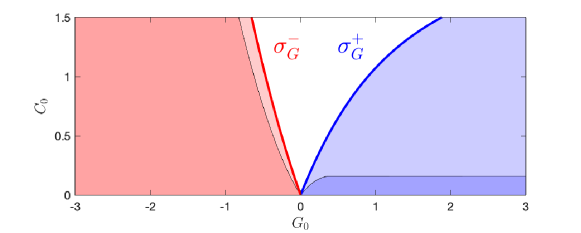
Figure 5. An illustration of the threshold regions for $(G_{0},C_{0})$ with parameters $\nu=.8,{\psi_{M}}=1,n=2$. Darker areas represent the rough conditions.

Remark 4.15.

The threshold curves $\sigma_{G}^{+}$ and $\sigma_{G}^{-}$ are dimension dependent. In the case $n=1$, one can check that $\sigma_{G}^{+}\equiv 0$ and $\sigma_{G}^{-}\equiv 0$. It recovers the sharp critical threshold condition in 1D, stated in Theorem 4.4.

For $n\geq 2$, we have $\sigma_{G}^{+}(x)>0$ and $\sigma_{G}^{-}(x)<0$ for $x>0$. There is a gap between the two regions, due to the nonlocal effect. The gap becomes larger as $n$ increases, illustrated in Figure 6. There is no gap when $C_{0}=0$ (when $\phi$ is a constant), regardless of the dimension.

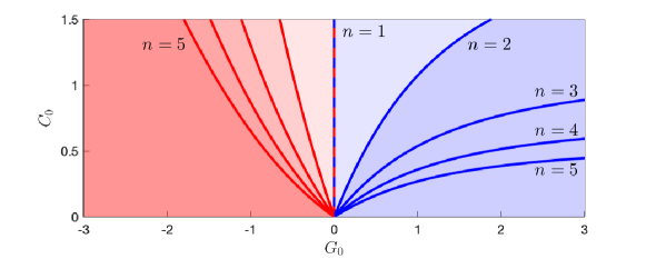
Figure 6. An illustration of threshold curves $\sigma_{G}^{+}$ and $\sigma_{G}^{-}$ in different dimensions $n=1,\cdots,5$, with parameters $\nu=.8,{\psi_{M}}=1$.

Finally, we wrap up the proof of Theorem 2.8.

Proof of Theorem 2.8.

For subcritical initial data, applying Propositions 4.9 and 4.14, we obtain the boundedness of $q$ and $G$. As $\psi$ is bounded (Proposition 4.7), we get $p=G-\psi$ is also bounded. Then, Proposition 2.1 implies the boundedness of $\nabla\mathbf{u}$, and global wellposedness is the direct consequence of Theorem 4.1. The asymptotic flocking behavior follows from Theorem 4.2.

For supercritical initial data, from Propositions 4.9 and 4.14, we deduce that either $q$ or $G$ blows up (which is equivalent to $p$ blows up due to the boundedness of $\psi$). Therefore, $\nabla\mathbf{u}$ becomes unbounded, resulting a loss of regularity in finite time. ∎

5. Further discussion

In this paper, we introduce a new pair of quantities $(u_{r},\frac{u}{r})$, which serve as a nice replacement of the 1D quantity $\partial_{x}u$, for pressure-less Eulerian dynamics in multi-dimensions with radial symmetry. The applications to the Euler-Poisson equations and the Euler-alignment equations show significant advantages of studying the dynamics of the pair, compared to the spectral dynamics (on eigenvalues of $\nabla\mathbf{u}$), as well as the divergence $\nabla\cdot\mathbf{u}$. The idea has the great potential to be applied to a large class of Eulerian dynamics with different forces.

There are several possible extensions.

1. Systems with pressure. Pressure appears naturally in many models of Eulerian dynamics. For the 1D Euler equation with isentropic pressure (known as the $p$-system), the Riemann invariants are introduced to handle the pressure. The quantities that are relevant to global regularity are $\partial_{x}(u\pm c(\rho))$, where $c(\rho)$ is the sound speed. Global regularity has been shown for the $p$-system [2] and the Euler-Poisson equations with pressure [19] in 1D. Global regularity in multi-dimensions is largely unknown. It is interesting to understand which quantities serve as a nice replacement of $\partial_{x}(u\pm c(\rho))$ in multi-dimensions with radial symmetry.

2. Radially symmetric flow with swirl. Radially symmetric solutions can allow swirls. For instance, in 2D, $u(\mathbf{x})=\frac{\mathbf{x}}{r}u(r)+\frac{\mathbf{x}^{\perp}}{r}R(r)$. It is known that rotations can prevent singularity formation [13]. Our global regularity result has the potential to be extended to radially symmetric data with swirl.

3. Perturbation around a radially symmetric solution. One next step is to study a non-symmetric perturbation around the radially symmetric solution. This would allow us to extend the result to a larger class of solutions.

We leave all these intriguing problems for further investigation.

References

- [1] José A Carrillo, Young-Pil Choi, Eitan Tadmor, and Changhui Tan. Critical thresholds in 1D Euler equations with non-local forces. Mathematical Models and Methods in Applied Sciences, 26(01):185–206, 2016.
- [2] Geng Chen. Optimal time-dependent lower bound on density for classical solutions of 1-D compressible Euler equations. Indiana University Mathematics Journal, 66(3):725–740, 2017.
- [3] Felipe Cucker and Steve Smale. Emergent behavior in flocks. Automatic Control, IEEE Transactions on, 52(5):852–862, 2007.
- [4] Tam Do, Alexander Kiselev, Lenya Ryzhik, and Changhui Tan. Global regularity for the fractional Euler alignment system. Archive for Rational Mechanics and Analysis, 228(1):1–37, 2018.
- [5] Shlomo Engelberg, Hailiang Liu, and Eitan Tadmor. Critical thresholds in Euler-Poisson equations. Indiana University Mathematics Journal, 50:109–157, 2001.
- [6] Alessio Figalli and Moon-Jin Kang. A rigorous derivation from the kinetic Cucker–Smale model to the pressureless euler system with nonlocal alignment. Analysis & PDE, 12(3):843–866, 2018.
- [7] Yan Guo. Smooth irrotational flows in the large to the Euler–Poisson system in . Communications in Mathematical Physics, 195(2):249–265, 1998.
- [8] Seung-Yeal Ha and Eitan Tadmor. From particle to kinetic and hydrodynamic descriptions of flocking. Kinetic and Related Models, 1(3):415–435, 2008.
- [9] Siming He and Eitan Tadmor. Global regularity of two-dimensional flocking hydrodynamics. Comptes Rendus Mathematique, 355(7):795–805, 2017.
- [10] Juhi Jang. The two-dimensional Euler-Poisson system with spherical symmetry. Journal of Mathematical Physics, 53(2):023701, 2012.
- [11] Juhi Jang, Dong Li, and Xiaoyi Zhang. Smooth global solutions for the two-dimensional Euler Poisson system. In Forum Mathematicum, volume 26, pages 645–701. De Gruyter, 2014.
- [12] Hailiang Liu and Eitan Tadmor. Spectral dynamics of the velocity gradient field in restricted flows. Communications in Mathematical Physics, 228(3):435–466, 2002.
- [13] Hailiang Liu and Eitan Tadmor. Rotation prevents finite-time breakdown. Physica D: Nonlinear Phenomena, 188(3-4):262–276, 2004.
- [14] Qianyun Miao, Changhui Tan, and Liutang Xue. Global regularity for a 1D Euler-alignment system with misalignment. arXiv preprint arXiv:2004.03652, 2020.
- [15] Roman Shvydkoy. Global existence and stability of nearly aligned flocks. Journal of Dynamics and Differential Equations, 31(4):2165–2175, 2019.
- [16] Roman Shvydkoy and Eitan Tadmor. Eulerian dynamics with a commutator forcing. Transactions of Mathematics and its Applications, 1(1):tnx001, 2017.
- [17] Eitan Tadmor and Hailiang Liu. Critical thresholds in 2D restricted Euler-Poisson equations. SIAM Journal on Applied Mathematics, 63(6):1889–1910, 2003.
- [18] Eitan Tadmor and Changhui Tan. Critical thresholds in flocking hydrodynamics with non-local alignment. Philosophical Transactions of the Royal Society of London A: Mathematical, Physical and Engineering Sciences, 372(2028):20130401, 2014.
- [19] Eitan Tadmor and Dongming Wei. On the global regularity of subcritical Euler–Poisson equations with pressure. Journal of the European Mathematical Society, 10(3):757–769, 2008.
- [20] Changhui Tan. On the Euler-alignment system with weakly singular communication weights. Nonlinearity, 33(4):1907, 2020.
- [21] Dehua Wang. Global solutions and relaxation limits of Euler-Poisson equations. Zeitschrift für angewandte Mathematik und Physik, 52(4):620–630, 2001.
- [22] Dongming Wei, Eitan Tadmor, and Hantaek Bae. Critical thresholds in multi-dimensional Euler-Poisson equations with radial symmetry. Communications in Mathematical Sciences, 10(1):75–86, 2012.