Distribution-Free Models of Social Networks

Abstract

The structure of large-scale social networks has predominantly been articulated using generative models, a form of average-case analysis. This chapter surveys recent proposals of more robust models of such networks. These models posit deterministic and empirically supported combinatorial structure rather than a specific probability distribution. We discuss the formal definitions of these models and how they relate to empirical observations in social networks, as well as the known structural and algorithmic results for the corresponding graph classes.

1 Introduction

Technological developments in the 21st century have given rise to large-scale social networks, such as the graphs defined by Facebook friendship relationships or followers on Twitter. Such networks arguably provide the most important new application domain for graph analysis in well over a decade.

1.1 Social Networks Have Special Structure

There is wide consensus that social networks have predictable structure and features, and accordingly are not well modeled by arbitrary graphs. From a structural viewpoint, the most well studied and empirically validated properties of social networks are:

1. A heavy-tailed degree distribution, such as a power-law distribution.

2. Triadic closure, meaning that pairs of vertices with a common neighbor tend to be directly connected—that friends of friends tend to be friends in their own right.

3. The presence of “community-like structures,” meaning subgraphs that are much more richly connected internally than externally.

4. The small-world property, meaning that it’s possible to travel from any vertex to any other vertex using remarkably few hops.

These properties are not generally possessed by Erdős-Rényi random graphs (in which each edge is present independently with some probability $p$); a new model is needed to capture them.

From an algorithmic standpoint, empirical results indicate that optimization problems are often easier to solve in social networks than in worst-case graphs. For example, lightweight heuristics are unreasonably effective in practice for finding the maximum clique or recovering dense subgraphs of a large social network.

The literature on models that capture the special structure of social networks is almost entirely driven by the quest for generative (i.e., probabilistic) models that replicate some or all of the four properties listed above. Dozens of generative models have been proposed, and there is little consensus about which is the “right” one. The plethora of models poses a challenge to meaningful theoretical work on social networks—which of the models, if any, is to be believed? How can we be sure that a given algorithmic or structural result is not an artifact of the model chosen?

This chapter surveys recent research on more robust models of large-scale social networks, which assume deterministic combinatorial properties rather than a specific generative model. Structural and algorithmic results that rely only on these deterministic properties automatically carry over to any generative model that produces graphs possessing these properties (with high probability). Such results effectively apply “in the worst case over all plausible generative models.” This hybrid of worst-case (over input distributions) and average-case (with respect to the distribution) analysis resembles several of the semi-random models discussed elsewhere in the book, such as in the preceding chapters on pseudorandom data (Chapter 26) and prior-independent auctions (Chapter 27).

Sections 2 and 3 of this chapter cover two models of social networks that are motivated by triadic closure, the second of the four signatures of social networks listed in Section 1. Sections 4 and 5 discuss two models motivated by heavy-tailed degree distributions.

2 Cliques of $c$-Closed Graphs

2.1 Triadic Closure

Triadic closure is the property that, when two members of a social network have a friend in common, they are likely to be friends themselves. In graph-theoretic terminology, two-hop paths tend to induce triangles.

Triadic closure has been studied for decades in the social sciences and there is compelling intuition for why social networks should exhibit strong triadic closure properties. Two people with a common friend are much more likely to meet than two arbitrary people, and are likely to share common interests. They might also feel pressure to be friends to avoid imposing stress on their relationships with their common friend.

The data support this intuition. Numerous large-scale studies on online social networks provide overwhelming empirical evidence for triadic closure. The plot in Figure 1, derived from the network of email communications at the disgraced energy company Enron, is representative. Other social networks exhibit similar triadic closure properties.

  

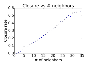
(a) Triadic closure in the Enron email network

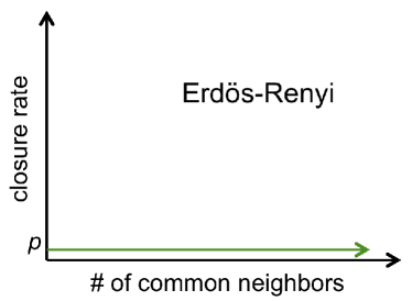
(b) Triadic closure in a random graph

Figure 1: In the Enron email graph, vertices correspond to Enron employees, and there is an edge connecting two employees if one sent at least one email to the other. In (a), vertex pairs of this graph are grouped according to the number of common neighbors (indicated on the $x$-axis). The $y$-axis shows the fraction of such pairs that are themselves connected by an edge. The edge density—the fraction of arbitrary vertex pairs that are directly connected—is roughly $10^{-4}$. In (b), a cartoon of the analogous plot for an Erdős-Rényi graph with edge density $p=10^{-4}$ is shown. Erdős-Rényi graphs are not a good model for networks like the Enron network—their closure rate is too small, and the closure rate fails to increase as the number of common neighbors increases.

2.2 $c$-Closed Graphs

The most extreme version of triadic closure would assert that whenever two vertices have a common neighbor, they are themselves neighbors: whenever $(u,v)$ and $(v,w)$ are in the edge set $E$, so is $(u,w)$. The class of graphs satisfying this property is not very interesting—it is precisely the (vertex-)disjoint unions of cliques—but it forms a natural base case for more interesting parameterized definitions.

Our first definition of a class of graphs with strong triadic closure properties is that of $c$-closed graphs.

Definition 2.1 (Fox et al. (2020)).

For a positive integer $c$, a graph $G=(V,E)$ is $c$-closed if, whenever $u,v\in V$ have at least $c$ common neighbors, $(u,v)\in E$.

For a fixed number of vertices, the parameter $c$ interpolates between unions of cliques (when $c=1$) and all graphs (when $c=|V|-1$). The class of 2-closed graphs—the graphs that do not contain a square (i.e., $K_{2,2}$) or a diamond (i.e., $K_{4}$ minus an edge) as an induced subgraph—is already non-trivial. The $c$-closed condition is a coarse proxy for the empirical closure rates observed in social networks (like in Figure 1), asserting that the closure rate jumps to 100% for vertices with $c$ or more common neighbors.

Next is a less stringent version of the definition, which is sufficient for the main algorithmic result of this section.

Definition 2.2 (Fox et al. (2020)).

For a positive integer $c$, a vertex $v$ of a graph $G=(V,E)$ is $c$-good if whenever $v$ has at least $c$ common neighbors with another vertex $u$, $(u,v)\in E$. The graph $G$ is weakly $c$-closed if every induced subgraph has at least one $c$-good vertex.

A $c$-closed graph is also weakly $c$-closed, as each of its vertices is $c$-good in each of its induced subgraphs. The converse is false; for example, a path graph is not 1-closed, but it is weakly 1-closed (as the endpoints of a path are 1-good). Equivalent to Definition 2.2 is the condition that the graph $G$ has an elimination ordering of $c$-good vertices, meaning the vertices can be ordered $v_{1},v_{2},\ldots,v_{n}$ such that, for every $i=1,2,\ldots,n$, the vertex $v_{i}$ is $c$-good in the subgraph induced by $v_{i},v_{i+1},\ldots,v_{n}$ (Exercise 1). Are real-world social networks $c$-closed or weakly $c$-closed for reasonable values of $c$? The next table summarizes some representative numbers.

	$n$	$m$	$c$	weak $c$
email-Enron	36692	183831	161	34
p2p-Gnutella04	10876	39994	24	8
wiki-Vote	7115	103689	420	42
ca-GrQc	5242	14496	41	9

Table 1: The $c$-closure and weak $c$-closure of four well-studied social networks from the SNAP (Stanford Large Network Dataset) collection of benchmarks (http://snap.stanford.edu/). “email-Enron” is the network described in Figure 1; “p2p-Gnutella04” is the topology of a Gnutella peer-to-peer network circa 2002; “wiki-Vote” is the network of who votes on whom in promotion cases on Wikipedia; and “ca-GrQc” is the collaboration network of authors of papers uploaded to the General Relativity and Quantum Cosmology section of arXiv. For each network $G$, $n$ indicates the number of vertices, $m$ the number of edges, $c$ the smallest value $\gamma$ such that $G$ is $\gamma$-closed, and “weak $c$” the smallest value $\gamma$ such that $G$ is weakly $\gamma$-closed.

These social networks are $c$-closed for much smaller values of $c$ than the trivial bound of $n-1$, and are weakly $c$-closed for quite modest values of $c$.

2.3 Computing a Maximum Clique: A Backtracking Algorithm

Once a class of graph has been defined, such as $c$-closed graphs, a natural agenda is to investigate fundamental optimization problems with graphs restricted to the class. We single out the problem of finding the maximum-size clique of a graph, primarily because it is one of the most central problems in social network analysis. In a social network, cliques can be interpreted as the most extreme form of a community.

The problem of computing the maximum clique of a graph reduces to the problem of enumerating the graph’s maximal cliques—the maximum clique is also maximal, so it appears as the largest of the cliques in the enumeration.

How does the $c$-closed condition help with the efficient computation of a maximum clique? We next observe that the problem of reporting all maximal cliques is polynomial-time solvable in $c$-closed graphs when $c$ is a fixed constant. The algorithm is based on backtracking. For convenience, we give a procedure that, for any vertex $v$, identifies all maximal cliques that contain $v$. (The full procedure loops over all vertices.)

1. Maintain a history $H$, initially empty.

2. Let $N$ denote the vertex set comprising $v$ and all vertices $w$ that are adjacent to both $v$ and all vertices in $H$.

3. If $N$ is a clique, report the clique $H\cup N$ and return.

4. Otherwise, recurse on each vertex $w\in N\setminus\{v\}$ with history $H:=H\cup\{v\}$.

This subroutine reports all maximal cliques that contain $v$, whether the graph is $c$-closed or not (Exercise 2). In a $c$-closed graph, the maximum depth of the recursion is $c$—once $|H|=c-1$, every pair of vertices in $N\setminus\{v\}$ has $c$ common neighbors (namely $H\cup\{v\}$) and hence $N$ must be a clique. The running time of the backtracking algorithm is therefore $n^{c+O(1)}$ in $c$-closed graphs.

This simplistic backtracking algorithm is extremely slow except for very small values of $c$. Can we do better?

2.4 Computing a Maximum Clique: Fixed-Parameter Tractability

There is a simple but clever algorithm that, for an arbitrary graph, enumerates all of the maximal cliques while using only polynomial time per clique.

Theorem 2.1 (Tsukiyama et al. (1977)).

There is an algorithm that, given any input graph with $n$ vertices and $m$ edges, outputs all of the maximal cliques of the graph in $O(mn)$ time per maximal clique.

Theorem 2.1 reduces the problem of enumerating all maximal cliques in polynomial time to the combinatorial task of proving a polynomial upper bound on the number of maximal cliques.

Computing a maximum clique of an arbitrary graph is an $NP$-hard problem, so presumably there exist graphs with an exponential number of maximal cliques. The Moon-Moser graphs are a simple and famous example. For $n$ a multiple of 3, the Moon-Moser graph with $n$ vertices is the perfectly balanced $\tfrac{n}{3}$-tite graph, meaning the vertices are partitioned into $\tfrac{n}{3}$ groups of 3, and every vertex is connected to every other vertex except for the 2 vertices in the same group (Figure 2).

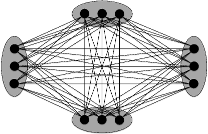
Figure 2: The Moon-Moser graph with $n=12$ vertices.

Choosing one vertex from each group induces a maximal clique, for a total of $3^{n/3}$ maximal cliques, and these are all of the maximal cliques of the graph. More generally, a basic result in graph theory asserts that no $n$-vertex graph can have more than $3^{n/3}$ maximal cliques.

Theorem 2.2 (Moon and Moser (1965)).

Every $n$-vertex graph has at most $3^{n/3}$ maximal cliques.

A Moon-Moser graph on $n$ vertices is not $c$-closed even for $c=n-3$, so there remains hope for a positive result for $c$-closed graphs with small $c$. The Moon-Moser graphs do show that the number of maximal cliques of a $c$-closed graph can be exponential in $c$ (since a Moon-Moser graph on $c$ vertices is trivially $c$-closed). Thus the best-case scenario for enumerating the maximal cliques of a $c$-closed graph is a fixed-parameter tractability result (with respect to the parameter $c$), stating that, for some function $f$ and constant $d$ (independent of $c$), the number of maximal cliques in an $n$-vertex $c$-closed graph is $O(f(c)\cdot n^{d})$. The next theorem shows that this is indeed the case, even for weakly $c$-closed graphs.

Theorem 2.3 (Fox et al. (2020)).

Every weakly $c$-closed graph with $n$ vertices has at most

$$3^{(c-1)/3}\cdot n^{2}$$

maximal cliques.

The following corollary is immediate from Theorems 2.1 and 2.3.

Corollary 2.3.1.

The maximum clique problem is polynomial-time solvable in weakly $c$-closed $n$-vertex graphs with $c=O(\log n)$.

2.5 Proof of Theorem 2.3

The proof of Theorem 2.3 proceeds by induction on the number of vertices $n$. (One of the factors of $n$ in the bound is from the $n$ steps in this induction.) Let $G$ be an $n$-vertex weakly $c$-closed graph. Assume that $n\geq 3$; otherwise, the bound is trivial.

By assumption, $G$ has a $c$-good vertex $v$. By induction, $G\setminus\{v\}$ has at most $(n-1)^{2}\cdot 3^{(c-1)/3}$ maximal cliques. (An induced subgraph of a weakly $c$-closed graph is again weakly $c$-closed.) Every maximal clique $C$ of $G\setminus\{v\}$ gives rise to a unique maximal clique in $G$ (namely $C$ or $C\cup\{v\}$, depending on whether the latter is a clique). It remains to bound the number of uncounted maximal cliques of $G$, meaning the maximal cliques $K$ of $G$ for which $K\setminus\{v\}$ is not maximal in $G\setminus\{v\}$.

An uncounted maximal clique $K$ must include $v$, with $K$ contained in $v$’s neighborhood (i.e., in the subgraph induced by $v$ and the vertices adjacent to it). Also, there must be a vertex $u\notin K$ such that $K\setminus\{v\}\cup\{u\}$ is a clique in $G\setminus\{v\}$; we say that $u$ is a witness for $K$, as it certifies the non-maximality of $K\setminus\{v\}$ in $G\setminus\{v\}$. Such a witness must be connected to every vertex of $K\setminus\{v\}$. It cannot be a neighbor of $v$, as otherwise $K\cup\{u\}$ would be a clique in $G$, contradicting $K$’s maximality.

Choose an arbitrary witness for each uncounted clique of $G$ and bucket these cliques according to their witness; recall that all witnesses are non-neighbors of $v$. For every uncounted clique $K$ with witness $u$, all vertices of the clique $K\setminus\{v\}$ are connected to both $v$ and $u$. Moreover, because $K$ is a maximal clique in $G$, $K\setminus\{v\}$ is a maximal clique in the subgraph $G_{u}$ induced by the common neighbors of $u$ and $v$.

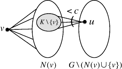
Figure 3: Proof of Theorem 2.3. $N(v)$ denotes the neighbors of $v$. $K$ denotes a maximal clique of $G$ such that $K\setminus\{v\}$ is not maximal in $G\setminus\{v\}$. There is a vertex $u$, not connected to $v$, that witnesses the non-maximality of $K\setminus\{v\}$ in $G\setminus\{v\}$. Because $v$ is a $c$-good vertex, $u$ and $v$ have at most $c-1$ common neighbors.

How big can such a subgraph $G_{u}$ be? This is the step of the proof where the weakly $c$-closed condition is important: Because $u$ is a non-neighbor of $v$ and $v$ is a $c$-good vertex, $u$ and $v$ have at most $c-1$ common neighbors and hence $G_{u}$ has at most $c-1$ vertices (Figure 3). By the Moon-Moser theorem (Theorem 2.2), each subgraph $G_{u}$ has at most $3^{(c-1)/3}$ maximal cliques. Adding up over the at most $n$ choices for $u$, the number of uncounted cliques is at most $n\cdot 3^{(c-1)/3}$; this sum over possible witnesses is the source of the second factor of $n$ in Theorem 2.3. Combining this bound on the uncounted cliques with the inductive bound on the remaining maximal cliques of $G$ yields the desired upper bound of

$$(n-1)^{2}\cdot 3^{(c-1)/3}+n\cdot 3^{(c-1)/3}\leq n^{2}\cdot 3^{(c-1)/3}.$$

3 The Structure of Triangle-Dense Graphs

3.1 Triangle-Dense Graphs

Our second graph class inspired by the strong triadic closure properties of social and information networks is the class of $\delta$-triangle-dense graphs. These are graphs where a constant fraction of vertex pairs having at least one common neighbor are directly connected by an edge. Equivalently, a constant fraction of the wedges (i.e., two-hop paths) of the graph belong to a triangle.

Definition 3.1 (Gupta et al. (2016)).

The triangle density of an undirected graph $G$ is $\tau(G):=3t(G)/w(G)$, where $t(G)$ and $w(G)$ denote the number of triangles and wedges of $G$, respectively. (We define $\tau(G)=0$ if $w(G)=0$.) The class of $\delta$-triangle-dense graphs consists of the graphs $G$ with $\tau(G)\geq\delta$.

(In the social networks literature, this is also called the transitivity or the global clustering coefficient.) Because every triangle of a graph contains 3 wedges, and no two triangles share a wedge, the triangle density of a graph is between 0 and 1—the fraction of wedges that belong to a triangle. Triangle density is another coarse proxy for the empirical closure rates observed in social networks (like in Figure 1(a)).

The 1-triangle-dense graphs are precisely the unions of disjoint cliques, while triangle-free graphs constitute the 0-triangle-dense graphs. The triangle density of an Erdős-Rényi graph with edge probability $p$ is concentrated around $p$ (cf., Figure 1(b)). For an Erdős-Rényi graph to have constant triangle density, one would need to set $p=\Omega(1)$. This would imply that the graph is dense, quite unlike social networks. For example, in the year 2011 the triangle density of the Facebook graph was computed to be $0.16$, which is five orders of magnitude larger than in a random graph with the same number of vertices (roughly 1 billion at the time) and edges (roughly 100 billion).

3.2 Visualizing Triangle-Dense Graphs

What do $\delta$-triangle-dense graphs look like? Can we make any structural assertions about them, akin to separator theorems for planar graphs (allowing them to be viewed as “approximate grids”) or the regularity lemma for dense graphs (allowing them to viewed as approximate unions of random bipartite graphs)?

Given that 1-triangle-dense graphs are unions of cliques, a first guess might be that $\delta$-triangle-dense graphs look like the approximate union of approximate cliques (as in Figure 4(a)). Such graphs certainly have high triangle density; could there be an “inverse theorem,” stating that these are in some sense the only graphs with this property?

In its simplest form, the answer to this question is “no,” as $\delta$-triangle-dense graphs become quite diverse once $\delta$ is bounded below 1. For example, adding a clique on $n^{2/5}$ vertices to an arbitrary bounded-degree $n$-vertex graph produces a $\delta$-triangle-dense graph with $\delta=1-o(1)$ as $n\rightarrow\infty$ (see Figure 4(b)).

    

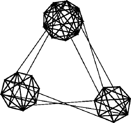
(a) An ideal triangle-dense graph

(b) The lollipop graph

Figure 4: Two examples of $\delta$-triangle-dense graphs with $\delta$ close to 1.

Nonetheless, an inverse theorem does hold if we redefine what it means to approximate a graph by a collection of approximate cliques. Instead of trying to capture most of the vertices or edges (which is impossible, as the previous example shows), we consider the goal of capturing a constant fraction of the triangles of a graph by a collection of dense subgraphs.

3.3 An Inverse Theorem

To state an inverse theorem for triangle-dense graphs, we require a preliminary definition.

Definition 3.2 (Tightly Knit Family).

Let $\rho>0$. A collection $V_{1},V_{2},\ldots,V_{k}$ of disjoint sets of vertices of a graph $G=(V,E)$ forms a $\rho$-tightly-knit family if:

1. For each $i=1,2,\ldots,k$, the subgraph induced by $V_{i}$ has at least $\rho\cdot\binom{|V_{i}|}{2}$ edges and $\rho\cdot\binom{|V_{i}|}{3}$ triangles. (That is, a $\rho$-fraction of the maximum possible edges and triangles.)

2. For each $i=1,2,\ldots,k$, the subgraph induced by $V_{i}$ has radius at most $2$.

In Definition 3.2, the vertex sets $V_{1},V_{2},\ldots,V_{k}$ are disjoint but need not cover all of $V$; in particular, the empty collection is technically a tightly knit family.

The following inverse theorem states that every triangle-dense graph contains a tightly-knit family that captures most of the “meaningful social structure”—a constant fraction of the graph’s triangles.

Theorem 3.1 (Gupta et al. (2016)).

There is a function $f(\delta)=O(\delta^{4})$ such that for every $\delta$-triangle dense graph $G$, there exists an $f(\delta)$-tightly-knit family that contains an $f(\delta)$ fraction of the triangles of $G$.

Graphs that are not triangle dense, such as sparse Erdős-Rényi random graphs, do not generally admit $\rho$-tightly-knit families with constant $\rho$. The complete tripartite graph shows that Theorem 3.1 does not hold if the “radius-2” condition in Definition 3.1 is strengthened to “radius-1” (Exercise 4).

3.4 Proof Sketch of Theorem 3.1

The proof of Theorem 3.1 is constructive, and interleaves two subroutines. To state the first, define the Jaccard similarity of an edge $(u,v)$ of a graph $G$ as the fraction of neighbors of $u$ and $v$ that are neighbors of both:

$$\frac{|N(u)\cap N(v)|}{|N(u)\cup N(v)|-2},$$

where $N(\cdot)$ denotes the neighbors of a vertex and the “-2” is to avoid counting $u$ and $v$ themselves. The first subroutine, called the cleaner, is given a parameter $\epsilon$ as input and repeatedly deletes edges with Jaccard similarity less than $\epsilon$ until none remain. Removing edges from the graph is worrisome because it removes triangles, and Theorem 3.1 promises that the final tightly knit family captures a constant fraction of the original graph’s triangles. But removing an edge with low Jaccard similarity destroys many more wedges than triangles, and the number of triangles in the graph is at least a constant fraction of the number of wedges (because it is $\delta$-triangle-dense). A charging argument along these lines shows that, provided $\epsilon$ is at most $\delta/4$, the cleaner cannot destroy more than a constant fraction of the graph’s triangles.

The second subroutine, called the extractor, is responsible for extracting one of the clusters of the tightly-knit family from a graph in which all edges have Jaccard similarity at least $\epsilon$. (Isolated vertices can be discarded from further consideration.) How is this Jaccard similarity condition helpful? One easy observation is that, post-cleaning, the graph is “approximately locally regular,” meaning that the endpoints of any edge have degrees within a $\tfrac{1}{\epsilon}$ factor of each other. Starting from this fact, easy algebra shows that every one-hop neighborhood of the graph (i.e., the subgraph induced by a vertex and its neighbors) has constant (depending on $\epsilon$) density in both edges and triangles, as required by Theorem 3.1. The bad news is that extracting a one-hop neighborhood can destroy almost all of a graph’s triangles (Exercise 4). The good news is that supplementing a one-hop neighborhood with a judiciously chosen subset of the corresponding two-hop neighborhood (i.e., neighbors of neighbors) fixes the problem. Precisely, the extractor subroutine is given a graph $G$ in which every edge has Jaccard similarity at least $\epsilon$ and proceeds as follows:

1. Let $v$ be a vertex of $G$ with the maximum degree. Let $d_{max}$ denote $v$’s degree and $N(v)$ its neighbors.

2. Calculate a score $\theta_{w}$ for every vertex $w$ outside $\{v\}\cup N(v)$ equal to the number of triangles that include $w$ and two vertices of $N(v)$. In other words, $\theta_{w}$ is the number of triangles that would be saved by supplementing the one-hop neighborhood $\{v\}\cup N(v)$ by $w$. (On the flip side, this would also destroy the triangles that contain $w$ and two vertices outside $N(v)$.)

3. Return the union of $\{v\}$, $N(v)$, and up to $d_{max}$ vertices outside $\{v\}\cup N(v)$ with the largest non-zero $\theta$-scores.

It is clear that the extractor outputs a set $S$ of vertices that induces a subgraph with radius at most 2. As with one-hop neighborhoods, easy algebra shows that, because every edge has Jaccard similarity at least $\epsilon$, this subgraph is dense in both edges and triangles. The important non-obvious fact, whose proof is omitted here, is that the number of triangles saved by the extractor (i.e., triangles with all three vertices in its output) is at least a constant fraction of the number of triangles it destroys (i.e., triangles with one or two vertices in its output). It follows that alternating between cleaning and extracting (until no edges remain) will produce a tightly-knit family meeting the promises of Theorem 3.1.

4 Power-Law Bounded Networks

Arguably the most famous property of social and information networks, even more so than triadic closure, is a power-law degree distribution, also referred to as a heavy-tailed or scale-free degree distribution.

4.1 Power-Law Degree Distributions and Their Properties

Consider a simple graph $G=(V,E)$ with $n$ vertices. For each positive integer $d$, let $n(d)$ denote the number of vertices of $G$ with degree $d$. The sequence $\{n(d)\}$ is called the degree distribution of $G$. Informally, a degree distribution is said to be a power-law with exponent $\gamma>0$ if $n(d)$ scales as $n/d^{\gamma}$.

There is some controversy about how to best fit power-law distributions to data, and whether such distributions are the “right” fit for the degree distributions in real-world social networks (as opposed to, say, lognormal distributions). Nevertheless, several of the consequences of a power-law degree distribution assumption are uncontroversial for social networks, and so a power-law distribution is a reasonable starting point for mathematical analysis.

This section studies the algorithmic benefits of assuming that a graph has an (approximately) power-law degree distribution, in the form of fast algorithms for fundamental graph problems. To develop our intuition about such graphs, let’s do some rough calculations under the assumption that $n(d)=cn/d^{\gamma}$ (for some constant $c$) for every $d$ up to the maximum degree $d_{max}$; think of $d_{max}$ as $n^{\beta}$ for some constant $\beta\in(0,1)$.

First, we have the implication

$$\sum_{d\leq d_{max}}n(d)=n\ \ \ \Longrightarrow\ \ \ cn\sum_{d\leq d_{max}}d^{-\gamma}=n.$$ (1)

When $\gamma\leq 1$, $\sum_{d<\infty}d^{-\gamma}$ is a divergent series. In this case, we cannot satisfy the right-hand side of (1) with a constant $c$. For this reason, results on power-law degree distributions typically assume that $\gamma>1$.

Next, the number of edges is exactly

$$\frac{1}{2}\sum_{d\leq d_{max}}d\cdot n(d)=\frac{cn}{2}\sum_{d\leq d_{max}}d^{-\gamma+1}.$$ (2)

Thus, up to constant factors, $\sum_{d\leq d_{max}}d^{-\gamma+1}$ is the average degree. For $\gamma>2$, $\sum_{d<\infty}d^{-\gamma+1}$ is a convergent series, and the graph has constant average degree. For this reason, much of the early literature on graphs with power-law degree distributions focused on the regime where $\gamma>2$. When $\gamma=2$, the average degree scales with $\log n$, and for $\gamma\in(1,2)$, it scales with $(d_{max})^{2-\gamma}$, which is polynomial in $n$.

One of the primary implications of a power-law degree distribution is upper bounds on the number of high-degree vertices. Specifically, under our assumption that $n(d)=cn/d^{\gamma}$, the number of vertices of degree at least $k$ can be bounded by

$$\sum_{d=k}^{d_{max}}n(d)\leq cn\sum_{d=k}^{\infty}d^{-\gamma}\leq cn\int^{\infty}_{k}x^{-\gamma}\,dx=cnk^{-\gamma+1}/(\gamma-1)=\Theta(nk^{-\gamma+1}).$$ (3)

4.2 PLB Graphs

The key definition in this section is a more plausible and robust version of the assumption that $n(d)=cn/d^{\gamma}$, for which the conclusions of calculations like those in Section 4.1 remain valid. The definition allows individual values of $n(d)$ to deviate from a true power law, while requiring (essentially) that the average value of $n(d)$ in sufficiently large intervals of $d$ does follow a power law.

Definition 4.1 (Berry et al. (2015); Brach et al. (2016)).

A graph $G$ with degree distribution $\{n(d)\}$ is a power-law bounded (PLB) graph with exponent $\gamma>1$ if there is a constant $c>0$ such that

$$\sum_{d=2^{r}}^{2^{r+1}}n(d)\leq cn\sum_{d=2^{r}}^{2^{r+1}}d^{-\gamma}$$

for all $r\geq 0$.

Many real-world social networks satisfy a mild generalization of this definition, in which $n(d)$ is allowed to scale with $n/(d+t)^{\gamma}$ for a “shift” $t\geq 0$; see the Notes for details. For simplicity, we continue to assume in this section that $t=0$.

Definition 4.1 has several of the same implications as a pure power law assumption, including the following lemma (cf. (2)).

Lemma 4.1.

Suppose $G$ is a PLB graph with exponent $\gamma>1$. For every $c>0$ and natural number $k$,

$$\sum_{d\leq k}d^{c}\cdot n(d)=O\left(n\sum_{d\leq k}d^{c-\gamma}\right).$$

The proof of Lemma 4.1 is technical but not overly difficult; we do not discuss the details here.

The first part of the next lemma provides control over the number of high-degree vertices and is the primary reason why many graph problems are more easily solved on PLB graphs than on general graphs. The second part of the lemma bounds the number of wedges of the graph when $\gamma\geq 3$.

Lemma 4.2.

Suppose $G$ is a PLB graph with exponent $\gamma>1$. Then:

• $\sum_{d\geq k}n(d)=O(nk^{-\gamma+1})$.

• Let $W$ denote the number of wedges (i.e., two-hop paths). If $\gamma=3$, $W=O(n\log n)$. If $\gamma>3$, $W=O(n)$.

Part (a) extends the computation in (3) to PLB graphs, while part (b) follows from Lemma 4.1 (see Exercise 5).

4.3 Counting Triangles

Many graph problems appear to be easier in PLB graphs than in general graphs. To illustrate this point, we single out the problem of triangle counting, which is one of the most canonical problems in social network analysis. For this section, we assume that our algorithms can determine in constant time if there is an edge between a given pair of vertices; these lookups can be avoided with a careful implementation (Exercise 6), but such details distract from the main analysis.

As a warm up, consider the following trivial algorithm to count (three times) the number of triangles of a given graph $G$ (“Algorithm 1”):

• For every vertex $u$ of $G$:

  • For every pair $v,w$ of $u$’s neighbors, check if $u$, $v$, and $w$ form a triangle.

Note that the running time of Algorithm 1 is proportional to the number of wedges in the graph $G$. The following running time bound for triangle counting in PLB graphs is an immediate corollary of Lemma 4.2(b), applied to Algorithm 1.

Corollary 4.0.1.

Triangle counting in $n$-vertex PLB graphs with exponent $3$ can be carried out in $O(n\log n)$ time. If the exponent is strictly greater than $3$, it can be done in $O(n)$ time.

Now consider an optimization of Algorithm 1 (“Algorithm 2”):

• Direct each edge of $G$ from the lower-degree endpoint to the higher-degree endpoint (breaking ties lexicographically) to obtain a directed graph $D$.

• For every vertex $u$ of $D$:

  • For every pair $v,w$ of $u$’s out-neighbors, check if $u$, $v$, and $w$ form a triangle in $G$.

Each triangle is counted exactly once by Algorithm 2, in the iteration where the lowest-degree of its three vertices plays the role of $u$. Remarkably, this simple idea leads to massive time savings in practice.

A classical way to capture this running time improvement mathematically is to parameterize the input graph $G$ by its degeneracy, which can be thought of as a refinement of the maximum degree. The degeneracy $\alpha(G)$ of a graph $G$ can be computed by iteratively removing a minimum-degree vertex (updating the vertex degrees after each iteration) until no vertices remain; $\alpha(G)$ is then the largest degree of a vertex at the time of its removal. (For example, every tree has degeneracy equal to 1.) We have the following guarantee for Algorithm 2, parameterized by a graph’s degeneracy:

Theorem 4.1 (Chiba and Nishizeki (1985)).

For every graph with $m$ edges and degeneracy $\alpha$, the running time of Algorithm 2 is $O(m\alpha)$.

Every PLB graph with exponent $\gamma>1$ has degeneracy $\alpha=O(n^{1/\gamma})$; see Exercise 8. For PLB graphs with $\gamma>2$, we can apply Lemma 4.1 with $c=1$ to obtain $m=O(n)$ and hence the running time of Algorithm 2 is $O(m\alpha)=O(n^{(\gamma+1)/\gamma})$.

Our final result for PLB graphs improves this running time bound, for all $\gamma\in(2,3)$, through a more refined analysis.

Theorem 4.2 (Brach et al. (2016)).

In PLB graphs with exponent $\gamma\in(2,3)$, Algorithm 2 runs in $O(n^{3/\gamma})$ time.

Proof.

Let $G=(V,E)$ denote an $n$-vertex PLB graph with exponent $\gamma\in(2,3)$. Denote the degree of vertex $v$ in $G$ by $d_{v}$ and its out-degree in the directed graph $D$ by $d^{+}_{v}$. The running time of Algorithm 2 is $O(n+\sum_{v}{d^{+}_{v}\choose 2})=O(n+\sum_{v}(d^{+}_{v})^{2})$, so the analysis boils down to bounding the out-degrees in $D$. One trivial upper bound is $d^{+}_{v}\leq d_{v}$ for every $v\in V$. Because every edge is directed from its lower-degree endpoint to its higher-degree endpoint, we also have $d^{+}_{v}\leq\sum_{d\geq d_{v}}n(d)$. By Claim 4.2(a), the second bound is $O(nd^{-\gamma+1}_{v})$. The second bound is better than the first roughly when $d_{v}\geq nd^{-\gamma+1}_{v}$, or equivalently when $d_{v}\geq n^{1/\gamma}$.

Let $V(d)$ denote the set of degree-$d$ vertices of $G$. We split the sum over vertices according to how their degrees compare to $n^{1/\gamma}$, using the first bound for low-degree vertices and the second bound for high-degree vertices:

$$\sum_{v\in V}(d^{+}_{v})^{2} = \sum_{d}\sum_{v\in V(d)}(d^{+}_{v})^{2}$$

$$\leq \sum_{d\leq n^{1/\gamma}}\sum_{v\in V(d)}d^{2}+\sum_{d>n^{1/\gamma}}\sum_{v\in V(d)}O(n^{2}d^{-2\gamma+2})$$

$$= \sum_{d\leq n^{1/\gamma}}d^{2}\cdot n(d)+O\left(n^{2}\cdot\sum_{d>n^{1/\gamma}}d^{-2\gamma+2}\cdot n(d)\right).$$

Applying Lemma 4.1 (with $c=2$) to the sum over low-degree vertices, and using the fact that with $\gamma<3$ the sum $\sum_{d}d^{2-\gamma}$ is divergent, we derive

$$\sum_{d\leq n^{1/\gamma}}d^{2}\cdot n(d)=O\left(n\sum_{d\leq n^{1/\gamma}}d^{2-\gamma}\right)=O(n(n^{1/\gamma})^{3-\gamma})=O(n^{3/\gamma}).$$

The second sum is over the highest-degree vertices, and Lemma 4.1 does not apply. On the other hand, we can invoke Claim 4.2(a) to obtain the desired bound:

$$n^{2}\sum_{d>n^{1/\gamma}}d^{-2\gamma+2}\cdot n(d) \leq n^{2}(n^{1/\gamma})^{-2\gamma+2}\sum_{d>n^{1/\gamma}}n(d)$$

$$= O(n^{2/\gamma}\cdot n(n^{1/\gamma})^{-\gamma+1})$$

$$= O(n^{3/\gamma}).$$

∎

The same reasoning shows that Algorithm 2 runs in $O(n\log n)$ time in $n$-vertex PLB graphs with exponent $\gamma=3$, and in $O(n)$ time in PLB graphs with $\gamma>3$ (Exercise 9).

4.4 Discussion

Beyond triangle counting, which computational problems should we expect to be easier on PLB graphs than on general graphs? A good starting point is problems that are relatively easy on bounded-degree graphs. In many cases, fast algorithms for bounded-degree graphs remain fast for graphs with bounded degeneracy. In these cases, the degeneracy bound for PLB graphs (Exercise 8) can already lead to fast algorithms for such graphs. For example, this approach can be used to show that all of the cliques of a PLB graph with exponent $\gamma>1$ can be enumerated in subexponential time (see Exercise 10). In some cases, like in Theorem 4.2, one can beat the bound from the degeneracy-based analysis through more refined arguments.

5 The BCT Model

This section gives an impressionistic overview of another set of deterministic conditions meant to capture properties of “typical networks,” proposed by Borassi et al. (2017) and hereafter called the BCT model. The precise model is technical with a number of parameters; we give only a high-level description that ignores several complications.

To illustrate the main ideas, consider the problem of computing the diameter $\max_{u,v\in V}\mathrm{dist}(u,v)$ of an undirected and unweighted $n$-vertex graph $G=(V,E)$, where $\mathrm{dist}(u,v)$ denotes the shortest-path distance between $u$ and $v$ in $G$. Define the eccentricity of a vertex $u$ by $\mathrm{ecc}(u):=\max_{v\in V}\mathrm{dist}(u,v)$, so that the diameter is the maximum eccentricity. The eccentricity of a single vertex can be computed in linear time using breadth-first search, which gives a quadratic-time algorithm for computing the diameter. Despite much effort, no subquadratic $(1+\epsilon)$-approximation algorithm for computing the graph diameter is known for general graphs. Yet there are many heuristics that perform well in real-world networks. Most of these heuristics compute the eccentricities of a carefully chosen subset of vertices. An extreme example is the TwoSweep algorithm:

1. Pick an arbitrary vertex $s$, and perform breadth-first search from $s$ to compute a vertex $t\in\operatorname*{arg\,max}_{v\in V}\mathrm{dist}(s,v)$.

2. Use breadth-first search again to compute $\mathrm{ecc}(t)$ and return the result.

This heuristic always produces a lower bound on a graph’s diameter, and in practice usually achieves a close approximation. What properties of “real-world” graphs might explain this empirical performance?

The BCT model is largely inspired by the metric properties of random graphs. To explain, for a vertex $s$ and natural number $k$, let $\tau_{s}(k)$ denote the smallest length $\ell$ so that there are at least $k$ vertices at distance (exactly) $\ell$ from $s$. Ignoring the specifics of the random graph model, the $\ell$-step neighborhoods (i.e., vertices at distance exactly $\ell$) of a vertex in a random graph resemble uniform random sets of size increasing with $\ell$. We next use this property to derive a heuristic upper bound on $\mathrm{dist}(s,t)$. Define $\ell_{s}:=\tau_{s}(\sqrt{n})$ and $\ell_{t}:=\tau_{t}(\sqrt{n})$. Since the $\ell_{s}$-step neighborhood of $s$ and the $\ell_{t}$-step neighborhood of $t$ act like random sets of size $\sqrt{n}$, a birthday paradox argument implies that they intersect with non-trivial probability. If they do intersect, then $\ell_{s}+\ell_{t}$ is an upper bound on $\mathrm{dist}(s,t)$. In any event, we can adopt this inequality as a deterministic graph property, which can be tested against real network data.

Property 5.1.

For all $s,t\in V$, $\mathrm{dist}(s,t)\leq\tau_{s}(\sqrt{n})+\tau_{t}(\sqrt{n})$.

One would expect this distance upper bound to be tight for pairs of vertices that are far away from each other, and in a reasonably random graph, this will be true for most of the vertex pairs. This leads us to the next property.

Property 5.2.

For all $s\in V$: for “most” $t\in V$, $\mathrm{dist}(s,t)>\tau_{s}(\sqrt{n})+\tau_{t}(\sqrt{n})-1$.

The third property posits a distribution on the $\tau_{s}(\sqrt{n})$ values. Let $T(k)$ denote the average $n^{-1}\sum_{s\in V}\tau_{s}(k)$.

Property 5.3.

There are constants $c,\gamma>0$ such that the fraction of vertices $s$ satisfying $\tau_{s}(\sqrt{n})\geq T(\sqrt{n})+\gamma$ is roughly $c^{-\gamma}$.

A consequence of this property is that the largest value of $\tau_{s}(\sqrt{n})$ is $T(\sqrt{n})+\log_{c}n+\Theta(1)$.

As we discuss below, these properties will imply that simple heuristics work well for computing the diameter of a graph. On the other hand, these properties do not generally hold in real-world graphs. The actual BCT model has a nuanced version of these properties, parameterized by vertex degrees. In addition, the BCT model imposes an approximate power-law degree distribution, in the spirit of power-law bounded graphs (Definition 4.1 in Section 4). This nuanced list of properties can be empirically verified on a large set of real-world graphs.

Nonetheless, for understanding the connection of metric properties to diameter computation, it suffices to look at Properties 5.1–5.3. We can now bound the eccentricities of vertices. The properties imply that

$$\mathrm{dist}(u,v)\leq\tau_{u}(\sqrt{n})+\tau_{v}(\sqrt{n})\leq\tau_{u}(\sqrt{n})+T(\sqrt{n})+\log_{c}n+O(1).$$

Fix $u$ and imagine varying $v$ to estimate $\mathrm{ecc}(u)$. For “most” vertices $v$, $\mathrm{dist}(u,v)\geq\tau_{u}(\sqrt{n})+\tau_{v}(\sqrt{n})-1$. By Property 5.3, one of the vertices $v$ satisfying this lower bound will also satisfy $\tau_{v}(\sqrt{n})\geq T(\sqrt{n})+\log_{c}n-\Theta(1)$. Combining, we can bound the eccentricity by

$$\mathrm{ecc}(u)=\max_{v}\mathrm{dist}(u,v)=\tau_{u}(\sqrt{n})+T(\sqrt{n})+\log_{c}n\pm\Theta(1).$$ (4)

The bound (4) is significant because it reduces maximizing $\mathrm{ecc}(u)$ over $u\in V$ to maximizing $\tau_{u}(\sqrt{n})$.

Pick an arbitrary vertex $s$ and consider a vertex $u$ that maximizes $\mathrm{dist}(s,u)$. By an argument similar to the one above (and because most vertices are far away from $s$), we expect that $\mathrm{dist}(s,u)\approx\tau_{s}(\sqrt{n})+\tau_{u}(\sqrt{n})$. Thus, a vertex $u$ maximizing $\mathrm{dist}(s,u)$ is almost the same as a vertex maximizing $\tau_{u}(\sqrt{n})$, which by (4) is almost the same as a vertex maximizing $\mathrm{ecc}(u)$. This gives an explanation of why the TwoSweep algorithm performs so well. Its first use of breadth-first search identifies a vertex $u$ that (almost) maximizes $\mathrm{ecc}(u)$. The second pass of breadth-first search (from $u$) then computes a close approximation of the diameter.

The analysis in this section is heuristic, but it captures much of the spirit of algorithm analysis in the BCT model. These results for TwoSweep can be extended to other heuristics that choose a set of vertices through a random process to lower bound the diameter. In general, the key insight is that most distances $\mathrm{dist}(u,v)$ in the BCT model can be closely approximated as a sum of quantities that depend only on either $u$ or $v$.

6 Discussion

Let’s take a bird’s-eye view of this chapter. The big challenge in the line of research described in this chapter is the formulation of graph classes and properties that both reflect real-world graphs and lead to a satisfying theory. It seems unlikely that any one class of graphs will simultaneously capture all the relevant properties of (say) social networks. Accordingly, this chapter described several graph classes that target specific empirically observed graph properties, each with its own algorithmic lessons:

• Triadic closure aids the computation of dense subgraphs.

• Power-law degree distributions aid subgraph counting.

• $\ell$-hop neighborhood structure influences the structure of shortest paths.

These lessons suggest that, when defining a graph class to capture “real-world” graphs, it may be important to keep a target algorithmic application in mind.

Different graph classes differ in how closely the definitions are tied to domain knowledge and empirically observed statistics. The $c$-closed and triangle-dense graph classes are in the spirit of classical families of graphs (e.g., planar or bounded-treewidth graphs), and they sacrifice precision in the service of generality, cleaner definitions, and arguably more elegant theory. The PLB and BCT frameworks take the opposite view: the graph properties are quite technical and involve many parameters, and in exchange tightly capture the properties of “real-world” graphs. These additional details can add fidelity to theoretical explanations for the surprising effectiveness of simple heuristics.

A big advantage of combinatorially defined graph classes—a hallmark of graph-theoretic work in theoretical computer science—is the ability to empirically validate them on real data. The standard statistical viewpoint taken in network science has led to dozens of competing generative models, and it is nearly impossible to validate the details of such a model from network data. The deterministic graph classes defined in this chapter give a much more satisfying foundation for algorithmics on real-world graphs.

Complex algorithms for real-world problems can be useful, but practical algorithms for graph analysis are typically based on simple ideas like backtracking or greedy algorithms. An ideal theory would reflect this reality, offering compelling explanations for why relatively simple algorithms have such surprising efficacy in practice.

We conclude this section with some open problems.

1. Theorem 2.3 gives, for constant $c$, a bound of $O(n^{2})$ on the number of maximal cliques in a $c$-closed graph. Fox et al. (2020) also prove a sharper bound of $O(n^{2(1-2^{-c})})$, which is asymptotically tight when $c=2$. Is it tight for all values of $c$? Additionally, parameterizing by the number of edges ($m$) rather than vertices ($n$), is the number of maximal cliques in a $c$-closed graph with $c=O(1)$ bounded by $O(m)$? Could there be a linear-time algorithm for maximal clique enumeration for $c$-closed graphs with constant $c$?

2. Theorem 3.1 guarantees the capture by a tightly-knit family of an $O(\delta^{4})$ fraction of the triangles of a $\delta$-triangle-dense graph. What is the best-possible constant in the exponent? Can the upper bound be improved, perhaps under additional assumptions (e.g., about the distribution of the clustering coefficients of the graph, rather than merely about their average)?

3. Ugander et al. (2013) observe that $4$-vertex subgraph counts in real-world graphs exhibit predictable and peculiar behavior. By imposing conditions on 4-vertex subgraph counts (in addition to triangle density), can one prove decomposition theorems better than Theorem 3.1?

4. Is there a compelling algorithmic application for graphs that can be approximated by tightly-knit families?

5. Benson et al. (2016) and Tsourakakis et al. (2017) defined the triangle conductance of a graph, where cuts are measured in terms of the number of triangles cut (rather than the number of edges). Empirical evidence suggests that cuts with low triangle conductance give more meaningful communities (i.e., denser subgraphs) than cuts with low (edge) conductance. Is there a plausible theoretical explanation for this observation?

6. A more open-ended goal is to use the theoretical insights described in this chapter to develop new and practical algorithms for fundamental graph problems.

7 Notes

The book by Easley and Kleinberg (2010) is a good introduction to social networks analysis, including discussions of heavy-tailed degree distributions and triadic closure. A good if somewhat outdated review of generative models for social and information networks is Chakrabarti and Faloutsos (2006). The Enron email network was first studied by Klimt and Yang (2004).

The definitions of $c$-closed and weakly $c$-closed graphs (Definitions 2.1–2.2) are from Fox et al. (2020), as is the fixed-parameter tractability result for the maximum clique problem (Theorem 2.3). Eppstein et al. (2010) proved an analogous result with respect to a different parameter, the degeneracy of the input graph. The reduction from efficiently enumerating maximal cliques to bounding the number of maximal cliques (Theorem 2.1) is from Tsukiyama et al. (1977). Moon-Moser graphs and the Moon-Moser bound on the maximum number of maximal cliques of a graph are from Moon and Moser (1965).

The definition of triangle-dense graphs (Definition 3.1) and the inverse theorem for them (Theorem 3.1) are from Gupta et al. (2016). The computation of the triangle density of the Facebook graph is detailed by Ugander et al. (2011).

The definition of power law bounded graphs (Definition 4.1) first appeared in Berry et al. (2015) in the context of triangle counting, but it was formalized and applied to many different problems by Brach et al. (2016), including triangle counting (Theorem 4.2), clique enumeration (Exercise 10), and linear algebraic problems for matrices with a pattern of non-zeroes that induces a PLB graph. Brach et al. (2016) also performed a detailed empirical analysis, validating Definition 4.1 (with small shifts $t$) on real data. The degeneracy-parameterized bound for counting triangles is essentially due to Chiba and Nishizeki (1985).

The BCT model (Section 5) and the fast algorithm for computing the diameter of a graph are due to Borassi et al. (2017).

Exercises

1. Prove that a graph is weakly $c$-closed in the sense of Definition 2.2 if and only if its vertices can be ordered $v_{1},v_{2},\ldots,v_{n}$ such that, for every $i=1,2,\ldots,n$, the vertex $v_{i}$ is $c$-good in the subgraph induced by $v_{i},v_{i+1},\ldots,v_{n}$.

2. Prove that the backtracking algorithm in Section 2.3 enumerates all of the maximal cliques of a graph.

3. Prove that a graph has triangle density $1$ if and only if it is a disjoint union of cliques.

4. Let $G$ be the complete regular tripartite graph with $n$ vertices—three vertex sets of size $\tfrac{n}{3}$ each, with each vertex connected to every vertex of the other two groups and none of the vertices within the same group.

   1. What is the triangle density of the graph?

   2. What is the output of the cleaner (Section 3.4) when applied to this graph? What is then the output of the extractor?

   3. Prove that $G$ admits no tightly-knit family that contains a constant fraction (as $n\rightarrow\infty$) of the graph’s triangles and uses only radius-1 clusters.

5. Prove Claim 4.2.

   [Hint: To prove (a), break up the sum over degrees into sub-sums between powers of $2$. Apply Definition 4.1 to each sub-sum.]

6. Implement Algorithm 2 from Section 4.3 in $O(\sum_{v}(d^{+}_{v})^{2}+n)$ time, where $d^{+}_{v}$ is the number of out-neighbors of $v$ in the directed version $D$ of $G$, assuming that the input $G$ is represented using only adjacency lists.

   [Hint: you may need to store the in- and out-neighbor lists of $D$.]

7. Prove that every graph with $m$ edges has degeneracy at most $\sqrt{2m}$. Exhibit a family of graphs showing that this bound is tight (up to lower order terms).

8. Suppose $G$ is a PLB graph with exponent $\gamma>1$.

   1. Prove that the maximum degree of $G$ is $O(n^{1/(\gamma-1)})$.

   2. Prove that the degeneracy is $O(n^{1/\gamma})$.

   [Hint: For (b), use the main idea in the proof of Exercise 7 and Claim 4.2.]

9. Prove that Algorithm 2 in Section 4.3 runs in $O(n\log n)$ time and $O(n)$ time in $n$-vertex PLB graphs with exponents $\gamma=3$ and $\gamma>3$, respectively.

10. Prove that all of the cliques of a graph with degeneracy $\alpha$ can be enumerated in $O(n2^{\alpha})$ time. (By Exercise 8(b), this immediately gives a subexponential-time algorithm for enumerating the cliques of a PLB graph.)

References

- Benson et al. (2016) Benson, A., D. F. Gleich, and J. Leskovec (2016). Higher-order organization of complex networks. Science 353(6295), 163–166.
- Berry et al. (2015) Berry, J. W., L. A. Fostvedt, D. J. Nordman, C. A. Phillips, C. Seshadhri, and A. G. Wilson (2015). Why do simple algorithms for triangle enumeration work in the real world? Internet Mathematics 11(6), 555–571.
- Borassi et al. (2017) Borassi, M., P. Crescenzi, and L. Trevisan (2017). An axiomatic and an average-case analysis of algorithms and heuristics for metric properties of graphs. In Proceedings of the Twenty-Eighth Annual ACM-SIAM Symposium on Discrete Algorithms (SODA), pp. 920–939.
- Brach et al. (2016) Brach, P., M. Cygan, J. Lacki, and P. Sankowski (2016). Algorithmic complexity of power law networks. In Proceedings of the Twenty-Seventh Annual ACM-SIAM Symposium on Discrete Algorithms (SODA), pp. 1306–1325.
- Chakrabarti and Faloutsos (2006) Chakrabarti, D. and C. Faloutsos (2006). Graph mining: Laws, generators, and algorithms. ACM Computing Surveys 38(1).
- Chiba and Nishizeki (1985) Chiba, N. and T. Nishizeki (1985). Arboricity and subgraph listing algorithms. SIAM Journal on Computing 14(1), 210–223.
- Easley and Kleinberg (2010) Easley, D. and J. Kleinberg (2010). Networks, Crowds, and Markets. Cambridge University Press.
- Eppstein et al. (2010) Eppstein, D., M. Löffler, and D. Strash (2010). Listing all maximal cliques in sparse graphs in near-optimal time. In Proceedings of the 21st International Symposium on Algorithms and Computation (ISAAC), pp. 403–414.
- Fox et al. (2020) Fox, J., T. Roughgarden, C. Seshadhri, F. Wei, and N. Wein (2020). Finding cliques in social networks: A new distribution-free model. SIAM Journal on Computing 49(2), 448–464.
- Gupta et al. (2016) Gupta, R., T. Roughgarden, and C. Seshadhri (2016). Decompositions of triangle-dense graphs. SIAM Journal on Computing 45(2), 197–215.
- Klimt and Yang (2004) Klimt, B. and Y. Yang (2004). The enron corpus: A new dataset for email classification research. In Proceedings of the 15th European Conference on Machine Learning (ECML), pp. 217–226.
- Moon and Moser (1965) Moon, J. and L. Moser (1965). On cliques in graphs. Israel Journal of Mathematics 3, 23–28.
- Roughgarden (2020) Roughgarden, T. (Ed.) (2020). Beyond the Worst-Case Analysis of Algorithms. Cambridge University Press.
- Tsourakakis et al. (2017) Tsourakakis, C. E., J. W. Pachocki, and M. Mitzenmacher (2017). Scalable motif-aware graph clustering. In Proceedings of the Web Conference (WWW), Volume abs/1606.06235, pp. 1451–1460.
- Tsukiyama et al. (1977) Tsukiyama, S., M. Ide, H. Ariyoshi, and I. Shirakawa (1977). A new algorithm for generating all the maximal independent sets. SIAM Journal on Computing 6(3), 505––517.
- Ugander et al. (2013) Ugander, J., L. Backstrom, and J. Kleinberg (2013). Subgraph frequencies: Mapping the empirical and extremal geography of large graph collections. In Proceedings of World Wide Web Conference, pp. 1307–1318.
- Ugander et al. (2011) Ugander, J., B. Karrer, L. Backstrom, and C. Marlow (2011). The anatomy of the facebook social graph. arXiv:1111.4503.