A scaling improved inner-outer decomposition of near-wall turbulent motions

Abstract

Near-wall turbulent velocities in turbulent channel flows are decomposed into small-scale and large-scale components at $y^{+}<100$ by improving the predictive inner-outer model of Baars et al. [Phys. Rev. Fluids 1, 054406 (2016)], where $y^{+}$ is the viscous-normalized wall-normal height. The small-scale one is obtained by reducing the outer reference height (a parameter in the model) from the center of the logarithmic layer to $y^{+}=100$, which can fully remove outer influences. On the other hand, the large-scale one represents the near-wall footprints of outer energy-containing motions. We present plenty of evidences that demonstrate that the small-scale motions are Reynolds-number invariant with the viscous scaling, at friction Reynolds numbers between 1000 and 5200. At lower Reynolds numbers from 180 to 600, the small scales can not be scaled by the viscous units, and the vortical structures are progressively strengthened as Reynolds number increases, which is proposed as a possible mechanism responsible for the anomalous scaling behavior. Finally, it is found that a small-scale part of the outer large-scale footprint can be well scaled by the viscous units.

I Introduction

Reynolds-number dependence and scaling laws for mean and fluctuating values of flow quantities have always been one of the most fundamental topics in turbulence research. For wall-bounded turbulent flows, the celebrated law of the wall for mean streamwise velocity is well known, albeit the debate on the logarithmic and the power laws [1]. For turbulence quantities, Townsend [2] proposed the attached eddy hypothesis (AEH) and predicted scaling relationships of fluctuating velocity variances at high-Reynolds-number condition, where it was postulated that the logarithmic layer of turbulent flow can be modelled as an ensemble of self-similar energy-containing eddies. The size and population density of these eddies are presumed to be proportional and inversely proportional to their wall normal height $y$ [3, 4, 5], respectively. There also exists a number of other theories in the literature that aim to predict the Reynolds-number effect and scaling laws of wall turbulence quantities [6, 7, 8]. In the near-wall region, it is now well recognized that the peak of streamwise turbulence intensity has a weak Reynolds number dependence when it is scaled by the friction velocity $u_{\tau}$ [9, 10], where $u_{\tau}=\sqrt{\overline{\tau}_{w}/\rho}$ ($\overline{\tau}_{w}$ is the mean wall-shear stress and $\rho$ is the fluid density). Although the mean flow is well accepted to follow the law of the wall, there is less consensus about the scaling of the Reynolds normal stresses, especially the Reynolds-number dependence of the near-wall peak and its physical origins.

Reynolds-number effect on near-wall turbulence statistics has been explored in many investigations over the past several decades. The classical view of wall-bounded turbulence considers an inner region near the wall where the viscous effect dominates, so that all velocity statistics should be universally scaled by the friction velocity and the kinematic viscosity of the fluid [11]. This is referred as the inner or viscous scaling that leads to the classical von Kármán’s law of the wall [12]. Although some studies seem to support this hypothesis [13, 14, 15, 16, 17], much more evidence definitely shows an increasing trend of the streamwise (inner) peak turbulence intensity with Reynolds number. The existence of Reynolds-number effect on near-wall turbulence intensities have been observed from numerous simulations and experiments in various types of canonical wall-bounded flows, including boundary layers, channels and pipes, which have provided strong evidence that near-wall turbulence statistics of fluctuating quantities do not follow the inner scaling [18, 19, 20, 21, 22, 23, 24, 9, 25, 26, 27, 28, 29, 30, 31, 32, 33, 34]. There have been some excellent reviews on the Reynolds-number scaling issue which provide much more historical details [35, 36, 37, 10].

In recent years, a prominent view is that the augmentation of near-wall turbulence intensities with Reynolds number can be attributed to the increasing influence of outer energetic motions in the inner region [25, 38, 39, 40]. As Reynolds number increases, very long and energy containing motions prevail in the logarithmic layer of wall-bounded turbulent flows, and they are conventionally termed as large-scale motions (LSMs), very-large-scale motions (VLSMs), superstructures or global modes [41, 42, 43, 44, 28, 45]. It was found that the turbulence kinetic energies carried by these structures increase with Reynolds number [27, 46, 28, 47]. Several studies [38, 39, 40] among others have clearly demonstrated that the aforementioned large outer energetic motions can penetrate deep down to the wall, playing as strong imprints or footprints, which is also consistent with Townsend’s AEH. As a consequence, the presence of large-scale footprints in the near-wall region can be associated with the failure of inner scaling of near-wall turbulence intensities [10].

On the other hand, another major progress recently in wall turbulence research is the discovery of a self-sustaining near-wall regeneration cycle, which comprises of quasi-cyclic regeneration of streaks and quasi-streamwise vortices [48, 49, 50, 51]. In this process, streaks can be profoundly amplified by quasi-streamwise vortices through transferring energy of mean shear to streamwise velocity fluctuations, i.e., the so-called lift-up effect [52, 53, 54, 55]. Then the amplified streaks rapidly oscillate and break down due to instability or transient growth, which in turn leads to the generation of new quasi-streamwise vortices [48, 51]. This cycle can also be uncovered via nonlinearly equilibrium or temporally periodic invariant solutions of the incompressible Navier-Stokes equations, which are termed by the exact coherent states as well [49, 50, 56]. In addition, the near-wall cycle is found to be autonomous in that it could be well self-sustained by artificially removing outer turbulent fluctuations [57]. Therefore, it should be reasonable to hypothesize that the statistics of the near-wall cycle can be completely scaled with the viscous units and thus Reynolds-number invariant [58], since it is now increasingly recognized that the Reynolds-number dependence of near-wall turbulence is solely introduced by outer footprints.

Based on the current understanding of near-wall turbulence, Marusic and co-workers proposed an algebraic predictive model for near-wall turbulence statistics with outer inputs [59, 58, 60], by incorporating the effects of superposition (footprints) and amplitude modulation of outer large scales on inner small-scale turbulent motions (near-wall cycle). Hence it suggests that outer footprints and near-wall autonomous cycle co-exist and interact in the near-wall region. In their model, a Reynolds-number-independent small-scale velocity component, namely $u^{*}$, is supposed to be a surrogate of the near-wall cycle and should be determined a priori in a calibration measurement. The model has been demonstrated to work well in turbulent boundary layers at $Re_{\tau}=2800\sim 19000$ [58, 60]. Here the friction Reynolds number is defined by $Re_{\tau}=u_{\tau}\delta/\nu$, $\delta$ is the outer length scale (boundary layer thickness, channel half height or pipe radius), and $\nu$ is the fluid kinematic viscosity.

However, there still exists several issues that should be addressed and clarified. The first and the most important one is, as a key component and assumption, explicit assessment of Reynolds-number invariance of $u^{*}$ was never put out, which is vital for the correctness of the model. Moreover, the predictive model is somewhat inconsistent with the attached eddy model [3, 5]. In the predictive model, the near-wall footprint is evaluated with an input large-scale velocity signal at $y_{O}^{+}=3.9\sqrt{Re_{\tau}}$ where the outer fluctuation is the strongest, and $y_{O}^{+}$ is the viscous-scaled wall-normal height of the input large-scale velocity signal, and $y^{+}$ is the viscous-scaled wall-normal height. However, the attached eddy model of Perry & Chong [3] admits the smallest self-similar wall-attached eddies of height $l_{y}^{+}\sim O(100)$ in viscous units, which is smaller than $3.9\sqrt{Re_{\tau}}$ at $Re_{\tau}>660$ and can also impose footprints in the near wall region. In other words, if $y_{O}^{+}=3.9\sqrt{Re_{\tau}}$ is used, the contributions of outer eddies with sizes of $l_{y}^{+}<3.9\sqrt{Re_{\tau}}$ are not accounted for footprints, thus the extracted $u^{*}$ is expected to be Reynolds number dependent, violating its elemental assumption. Furthermore, in practical implementation of the model, Mathis et al. [58] claimed that the Fourier phases of the large-scale signal in the calibration measurement need to be retained and replace the large-scale velocity phases measured under the prediction condition. Without this procedure, one-point moments, especially high order ones, would be erroneously predicted. This indicates that the extracted universal signal $u^{*}$ may still contain a fraction of outer large-scale footprints [58]. The above mentioned inconsistency or nonphysical manipulation, may be closely related to the Reynolds number dependence of $u^{*}$.

Moreover, there are some other relevant studies that tried to extract universal near-wall turbulence. Hwang [61] designed numerical experiments that the near-wall turbulent motions with $\lambda_{z}^{+}>100$ at $Re_{\tau}$ up to 660 were removed using the spanwise minimum flow unit (MFU) [62], $\lambda_{z}^{+}$ is the viscous-scaled spanwise wavelength. It was found that the streamwise velocity fluctuations at $y^{+}<40$ are well scaled by the viscous units, whereas the wall-normal and spanwise velocity fluctuations are not. Yin et al. [63] extended the work of Hwang [61] to higher Reynolds numbers, i.e, $Re_{\tau}=1000\sim 4000$, confirming similar findings. Then Yin et al. [64] modified the predictive model of Marusic and co-workers by replacing experimentally calibrated $u^{*}$ with three-dimensional turbulent velocity fields obtained from MFU simulation. Yin et al. [64] also compared the intensities of the extracted $(u^{*},v^{*},w^{*})$ from the predictive model and MFU, and found good agreements, while the comparison was taken only at a single not a wide range of Reynolds number. Agostini, Leschziner and others [65, 66] employed the ”Empirical Mode Decomposition” method to extract the small-scale motions, however they also did not explicitly demonstrate its $Re_{\tau}$ independence. Hearst et al. [67] utilized a windowing technique to extract the universal inner small-scale spectrum measured from turbulent boundary layers subjected to high-intensity freestream turbulence, but they did not apply this method to instantaneous flow field. Carney et al. [68] proposed an interesting near-wall patch approach, while which needs explicit high-pass filtering to obtain Reynolds-number invariant solutions.

In the present study, we firstly check whether the $u^{*}$ (as well as $v^{*}$ and $w^{*}$) extracted by adopting the refined predictive model of Baars et al. [60] is statistically Reynolds number independent in the Reynolds number range of $180\leq Re_{\tau}\leq 5200$. And it is indeed found that the statistics of the extracted $u^{*}$, $v^{*}$ and $w^{*}$ are definitely Reynolds number dependent, due to the fact that the outer eddies of $100<l_{y}^{+}<3.9\sqrt{Re_{\tau}}$ should be further included to calculate the footprints. Therefore, we simply let $y_{O}^{+}=100$ and extract $u^{*}$, $v^{*}$ and $w^{*}$ with negligible Reynolds number dependence in turbulent channel flows at $Re_{\tau}=1000\sim 5200$ using high-fidelity DNS data, which may help to further improve the predictive model for near-wall turbulence, or shed light on the physics of interactions of turbulent motions with different scales.

The paper is organised as follows. In §2, the data sets used in this work are described. In §3, we outline the decomposition scheme all three velocity components. Section §4 shows the evidence for Reynolds-number-independent small-scale motions in the Reynolds number range of $Re_{\tau}=1000\sim 5200$. The low-Reynolds-number effect at $Re_{\tau}=180\sim 600$ is given in §5, as well as the characteristics and scalings of large-scale outer footprints in §6. The final conclusion of the paper is drawn in §7. In this paper, the streamwise ($x$), wall-normal ($y$), and spanwise ($z$) velocity fluctuations are denoted as $u$, $v$ and $w$, respectively. The superscript ’$+$’ indicates the viscous scaling, i.e. the normalization by the friction velocity $u_{\tau}$ and the kinematic viscosity $\nu$. The angle brackets represent the spatio-temporal averaging in each of the homogeneous directions and in time.

II Data sets

The main data sets used in this study are from DNS (direct numerical simulation) of fully developed turbulent channel flows. The friction Reynolds numbers are $Re_{\tau}=180$, 310, 600, 1000, 2000 and 5200, covering a wide range over at least one order of magnitude, which could help to display the Reynolds number effect on the near-wall turbulence clearly.

Table 1: Summary of the DNS data sets. The $Re_{\tau}=180\sim 600$ data are from our own DNS, the $Re_{\tau}=1000$ and $Re_{\tau}=5200$ data are from Lee & Moser [32] indicated by LM15, and the $Re_{\tau}=2000$ data are from Hoyas & Jiménez [27] indicated by HJ06. $L_{x}$ and $L_{z}$ are computation domain sizes in streamwise and spanwise, respectively. The outer length scale, i.e., boundary-layer thickness, channel half height or pipe radius, is denoted by $\delta$. $\Delta x^{+}$ and $\Delta z^{+}$ are the streamwise and spanwise viscous-scaled grid size. $\Delta y^{+}_{w}$ and $\Delta y^{+}_{c}$ are the viscous-scaled wall-normal grid spacings at the wall and the channel centre, respectively. FD denotes finite difference scheme, and SP denotes spectral method.

$Re_{\tau}$	Reference	Method	$L_{x}/\delta$	$L_{z}/\delta$	$\Delta x^{+}$	$\Delta z^{+}$	$\Delta y^{+}_{w}$	$\Delta y^{+}_{c}$	Line and Symbol
180	Present	FD	8$\pi$	3$\pi$	10	4.99	0.196	7.08	$\minus$$\medblackcircle$$\minus$
310	Present	FD	6$\pi$	2$\pi$	10	5.00	0.270	9.84	$\minus$$\medblackdiamond$$\minus$
600	Present	FD	4$\pi$	2$\pi$	10	5.00	0.325	11.97	$\minus$$\medblacktriangleup$$\minus$
1000	LM15 [32]	SP	8$\pi$	3$\pi$	12.3	6.14	0.017	6.16	$\minus$$\medblacktriangledown$$\minus$
2000	HJ06 [27]	SP	8$\pi$	3$\pi$	8.2	4.09	0.323	8.89	$\minus$$\medblacktriangleright$$\minus$
5200	LM15 [32]	SP	8$\pi$	3$\pi$	12.8	6.38	0.498	10.3	$\minus$$\medblackstar$$\minus$

The turbulent channel data sets at $Re_{\tau}$=180, 310 and 600 are obtained from the DNS by ourselves. The DNS code adopts a fourth-order accurate compact difference scheme in the homogeneous directions and a second-order accurate central difference scheme in the wall-normal direction for the descretization of the incompressible Navier-Stokes equations on a staggered grid [69]. In our previous work, a series of low-Reynolds-number channel DNS (up to $Re_{\tau}=180$) were conducted using the code [70] and the results were well validated against Lee & Moser [32]. In this study, we perform simulations at two higher Reynolds numbers, i.e. $Re_{\tau}=310$ and 600, following the same standard at the lower Reynolds numbers, which is validated with Lee & Moser [32] at similar Reynolds numbers in Appendix A. The DNS data sets of channel flows at $Re_{\tau}$ = 1000 and 5200 were computed by the group at The University of Texas at Austin (UTA) [32], the raw data of which are assessed from the Johns Hopkins Turbulence Database (JHTDB) [71]. And the data set at $Re_{\tau}=2000$ was generated and assessed from the group at Universidad Politécnica de Madrid (UPM) [27]. All the cases of $Re_{\tau}=1000$, 2000 and 5200 were solved using spectral method in the wall-parallel planes, and the UTA group adopted a 7th-order B-spline collocation method while the UPM group employed a seven-point compact finite difference scheme in the wall-normal direction. The detailed information of the data sets is listed in table 1.

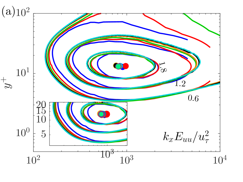
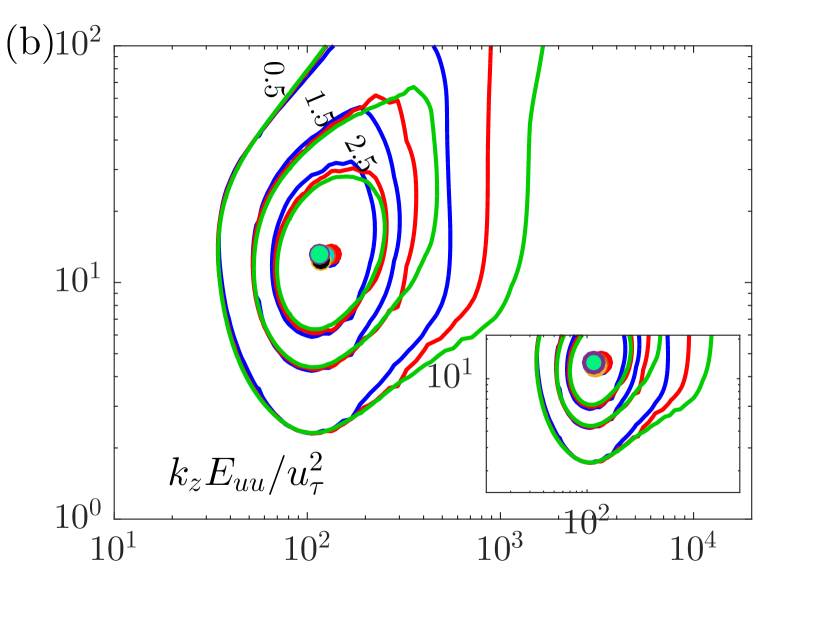
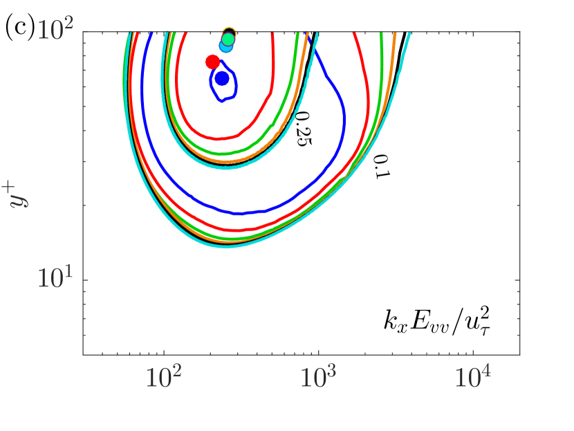
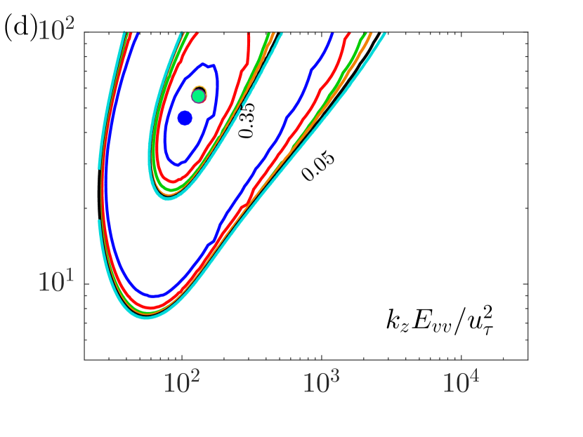
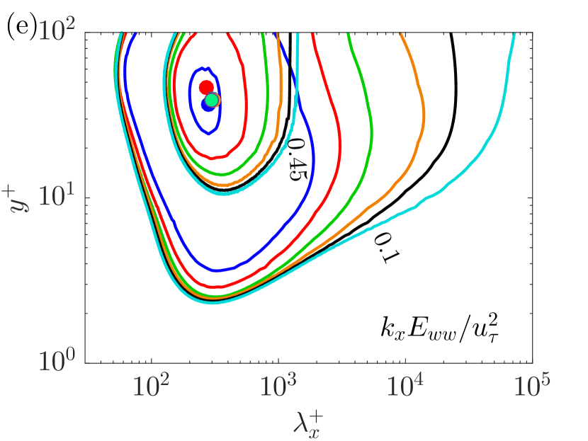
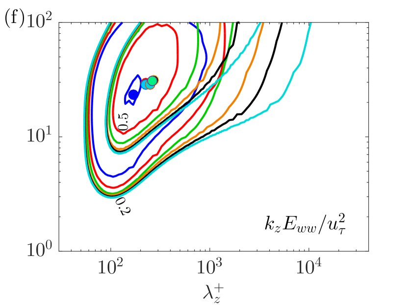
Figure 1: Pre-multiplied energy spectra of the three velocity components at different Reynolds numbers in the near-wall region ($y^{+}<100$). Lines with different colors correspond to different Reynolds numbers, see table 1. (a) $k_{x}E_{uu}/u_{\tau}^{2}$, (b) $k_{z}E_{uu}/u_{\tau}^{2}$, (c) $k_{x}E_{vv}/u_{\tau}^{2}$, (d) $k_{z}E_{vv}/u_{\tau}^{2}$, (e) $k_{x}E_{ww}/u_{\tau}^{2}$ and (f) $k_{z}E_{ww}/u_{\tau}^{2}$. The locations of inner spectral peaks have been marked with symbols and zoomed areas for the small-scale signal in the near wall-region.

FIG 1 shows the viscous-scaled streamwise and spanwise pre-multiplied energy spectra of the three components of velocity fluctuations in the near-wall region, i.e. $y^{+}<100$. It is seen that distinct inner peaks can be clearly observed, which are the spectral signatures of predominant near-wall coherent structures (streaks, quasi-streamwise vortices, etc) with specific characteristic length scales. The streamwise and spanwise pre-multiplied energy spectra of streamwise velocity fluctuations at $Re_{\tau}=180\sim 5200$ are shown in FIG 1 (a) and (b). $k_{x}E_{u_{i}u_{i}}(\lambda_{x}^{+},y^{+})=k_{x}\langle\hat{u_{i}}^{+}(\lambda_{x}^{+},y^{+},z^{+},t^{+})\overline{\hat{u_{i}}^{+}(\lambda_{x}^{+},y^{+},z^{+},t^{+})}\rangle$, where $<>$ denotes the average in time and in the spanwise direction, $\hat{u_{i}}$ is the Fourier coefficients of $u_{i}$ along $x$ direction (i = 1,2,3 for $u$, $v$, $w$) and the overbar indicates complex conjugate, $k_{x}=2\pi/\lambda_{x}$ and $\lambda_{x}$ is streamwise wavenumber. So did the spanwise wavenumber pre-multiplied energy spectra. The inner peak (marked with symbols in FIG 1 (a) for $Re_{\tau}$ = 180 and 5200) locates at $y^{+}=10\sim 20$, with $\lambda_{x}^{+}\sim O(10^{3})$ and $\lambda_{z}^{+}\sim O(10^{2})$, which is consistent with the well known characteristic streamwise length and spanwise spacing of near-wall streaks obtained from measurements or DNS [72, 73, 74]. The spectra of wall-normal and spanwise velocity components are displayed in FIG 1 (c-f). It is seen that the inner peaks of $v$- and $w$-spectra locate at $y^{+}=30\sim 70$ (except for $k_{x}E_{vv}$, where the higher Reynolds number inner peak positions are close to 100), since $v$ and $w$ are primarily induced by quasi-streamwise vortical structures which generally ride above the near-wall streaks [75, 61, 76]. For the small scales in the near-wall region (e.g., $\lambda_{x}^{+}<\sim 7000$ or $\lambda_{z}^{+}<\sim 200$ for the $u$-spectra), we can see that the spectra at $Re_{\tau}\geq 1000$ collapse generally well, shown in the zoomed area in FIG 1 (a,b), indicating Reynolds-number-independent near-wall small-scale turbulent motions [61, 32, 67, 77]. However, the spectra can not be well collapsed with viscous scaling at $Re_{\tau}=180\sim 600$ of the small-scale signal in the near wall-region, especially for the $v$- and $w$-spectra, indicating possible low-Reynolds-number effect in this Reynolds number range. The spectral imprints of outer large-scale components into the near-wall region are stronger and extending to longer wavelength with viscous scaling for $u$ and $w$ if $Re_{\tau}$ is larger, demonstrating increasing outer influences, which has been well known according to many previous works [25, 38, 39, 40, 78, 79, 80].

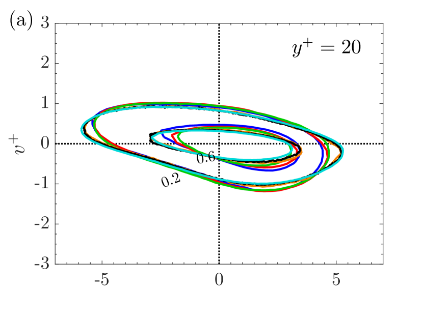
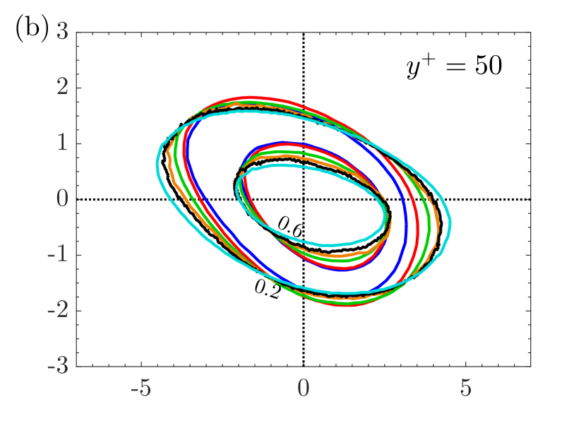
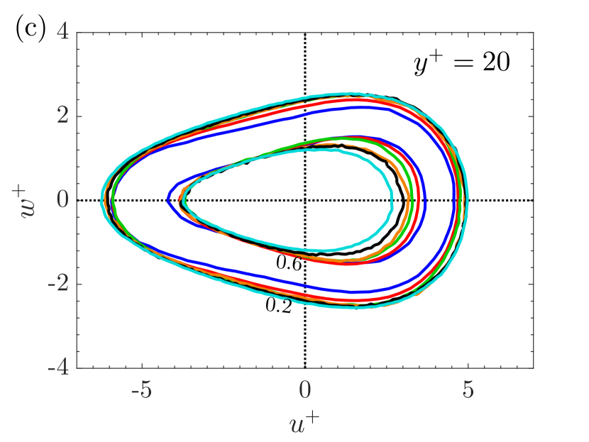
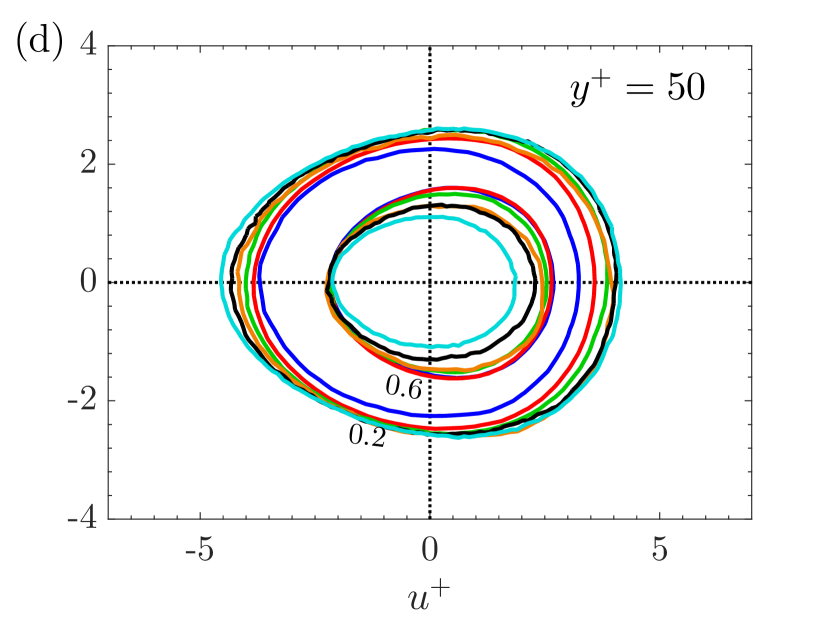
Figure 2: Joint p.d.f.s $P(u^{+},v^{+})$ (a, b) and $P(u^{+},w^{+})$ (c, d) at $y^{+}$ = 20 (a, c) and $y^{+}$ = 50 (b, d) in the fully developed turbulent channel flows at the Reynolds numbers $Re_{\tau}=180\sim 5200$. Lines with different colors correspond to different Reynolds numbers, see table 1. The contour levels are normalized by the peak value of the p.d.f.

The joint probability distribution function (p.d.f.) between velocity components is a useful tool related to the quadrant analysis, which was proposed nearly fifty years before and has been thoroughly adopted to detect the outward (Q1, $u>0$ and $v>0$), ejection (Q2, $u<0$ and $v>0$), inward (Q3, $u<0$ and $v<0$) and sweep (Q4, $u>0$ and $v<0$) events [81, 82, 83, 84]. As displayed in FIG 2 (a, b), the shape of $P(u^{+},v^{+})$ is inclined with the major axis in the Q2-Q4 direction, implying much higher probabilities of the ejection and sweep events. The p.d.f. contours at the two heights both show Reynolds number dependence, and the major axis tends to $v^{+}=0$ if $Re_{\tau}$ increases, which indicates $u^{+}$ increases more rapidly than $v^{+}$. If comparing the p.d.f.s at the two heights, i.e. $y^{+}=20$ and $y^{+}=50$ in FIG 2 (a) and (b), it can be seen that the inclination of the major axis is steeper at $y^{+}=50$, that means the ejecting and sweeping angles of coherent motions are smaller towards the wall. FIG 2 (c, d) demonstrates that the shape of $P(u^{+}$, $w^{+})$ is symmetric about $w^{+}=0$ in all cases. However, the p.d.f.s are not symmetric about $u^{+}=0$, showing quite different velocity distributions at $u>0$ and $u<0$. In general, the spanwise velocity $w$ has a wider distribution at $u>0$ than $u<0$. This is probably due to the splatting effect [65, 66, 85] or the dispersive motions of high-speed structures [86], i.e., high-speed sweeping (Q4) motions (mainly $u$ component) may be partly converted into spanwise motions ($w$ component) near the wall. The splatting/dispersive effect becomes weaker away from the wall, which could be confirmed in FIG 2 (d). Also, there exists visible Reynolds number dependence of $P(u^{+}$, $w^{+})$. Also, some modern developments of the quadrant analysis have been applied to reveal the spatial organization and time evolution of sweeps and ejections [87, 88, 89, 90].

In summary, we have presented some statistics (pre-multiplied energy spectra and joint p.d.f.s) of the channel flow DNS data in the near-wall region, covering a wide range of Reynolds numbers at $Re_{\tau}=180\sim 5200$. From the spectra, we found that the near-wall small-scale turbulence may be Reynolds number independent at $Re_{\tau}\geq 1000$, while which is Reynolds number dependent at $Re_{\tau}=180\sim 600$. However, there are very few attempts to extract the part of the flow which should be Reynolds number independent. In the following, we will employ the above DNS data to work out the decomposition of near-wall turbulent motions and verify whether the extracted $(u^{*},v^{*},w^{*})$ are really Reynolds number independent.

III Decomposition methodology

The decomposition of near-wall turbulent motions is based on the framework of the predictive inner-outer (PIO) model proposed by Marusic and co-workers [59, 58]. The basic idea of the PIO model is that the near-wall turbulence fluctuations could be decomposed into two components, i.e., the footprints of outer large-scale fluctuations (the superposition effect), and the small-scale fluctuations with modulated amplitudes by large scales (the modulation effect). Here we resort to the refined PIO model of Baars et al. [60], which eliminates the need for a specific spectral cut-off filter to separate small- and large-scale velocities as in the original version of this model.

The refined PIO model proposed for streamwise velocity takes the form of

$${\color[rgb]{0,0,0}u^{+}_{p}(x^{+},y^{+},z^{+},t^{+})=\underbrace{u^{*}(x^{+},y^{+},z^{+},t^{+})\left[1+\Gamma_{uu}(y^{+})u_{L}^{+}(x^{+},y^{+},z^{+},t^{+})\right]}_{\textbf{modulation}}+\underbrace{u_{L}^{+}(x^{+},y^{+},z^{+},t^{+})}_{\textbf{superposition}}.}$$ (1)

Here $u_{p}^{+}$ is the predicted streamwise fluctuating velocity near the wall. All of the variables are normalized by the viscous units. In the right-hand-side of equation (1), $\Gamma_{uu}(y^{+})$ is the modulation coefficient and $u^{*}(x^{+},y^{+},z^{+},t^{+})$ is the near-wall Reynolds number independent signal in the absence of outer influence, which are usually determined through a synchronously two-point calibration experiment, and assumed to be $Re_{\tau}$ independent [58, 60]. Where the second term $u_{L}^{+}(x^{+},y^{+},z^{+},t^{+})$ denotes the large-scale component of streamwise velocity fluctuation in the near wall region. Here we also follow Baars et al. [60] to calculate the outer footprint of streamwise velocity $u_{L}^{+}(x^{+},y^{+},z^{+},t^{+})$ as

$${\color[rgb]{0,0,0}u_{L}^{+}(x^{+},y^{+},z^{+},t^{+})=F_{x}^{-1}\{H_{Lu}(\lambda_{x}^{+},y^{+})F_{x}[u_{O}^{+}(x^{+},y_{O}^{+},z^{+},t^{+})]\},}$$ (2)

and the large-scale footprints $v_{L}$ and $w_{L}$ are obtained similar to $u_{L}^{+}(x^{+},y^{+},z^{+},t^{+})$ [64], i.e.,

$${\color[rgb]{0,0,0}v_{L}^{+}(x^{+},y^{+},z^{+},t^{+})=F_{x}^{-1}\{H_{Lv}(\lambda_{x}^{+},y^{+})F_{x}[v_{O}^{+}(x^{+},y_{O}^{+},z^{+},t^{+})]\},}$$ (3)

$${\color[rgb]{0,0,0}w_{L}^{+}(x^{+},y^{+},z^{+},t^{+})=F_{x}^{-1}\{H_{Lw}(\lambda_{x}^{+},y^{+})F_{x}[w_{O}^{+}(x^{+},y_{O}^{+},z^{+},t^{+})]\},}$$ (4)

in which, $u_{O}^{+},v_{O}^{+}$ and $w_{O}^{+}$ are the input outer fluctuating velocity at $y_{O}^{+}$ and $y_{O}^{+}=3.9\sqrt{Re_{\tau}}$ is usually used to approximate the centre of the logarithmic layer which also corresponds to the location of the outer spectral peak [58, 60]. By checking the exact locations of the outer spectral peaks at $Re_{\tau}=2000$ and 5200 [28, 91], we found the approximation $y_{O}^{+}=3.9\sqrt{Re_{\tau}}$ is quite accurate. $F_{x}$ and $F_{x}^{-1}$ denote FFT and inverse FFT, respectively. In equation (2-4), $H_{Lu}$, $H_{Lv}$ and $H_{Lw}$ are scale-dependent complex-valued kernel functions for calculating footprints, representing the spectral linear stochastic estimation of outer velocity components in the near-wall region, defined by

$${\color[rgb]{0,0,0}H_{Lu}(\lambda_{x}^{+},y^{+})=\frac{\langle\hat{u}^{+}(\lambda_{x}^{+},y^{+},z^{+},t^{+})\overline{\hat{u}^{+}(\lambda_{x}^{+},y_{O}^{+},z^{+},t^{+})}\rangle}{\langle\hat{u}^{+}(\lambda_{x}^{+},y_{O}^{+},z^{+},t^{+})\overline{\hat{u}^{+}(\lambda_{x}^{+},y_{O}^{+},z^{+},t^{+})}\rangle}=|H_{Lu}|e^{j\phi_{u}},}$$ (5)

$${\color[rgb]{0,0,0}H_{Lv}(\lambda_{x}^{+},y^{+})=\frac{\langle\hat{v}^{+}(\lambda_{x}^{+},y^{+},z^{+},t^{+})\overline{\hat{v}^{+}(\lambda_{x}^{+},y_{O}^{+},z^{+},t^{+})}\rangle}{\langle\hat{v}^{+}(\lambda_{x}^{+},y_{O}^{+},z^{+},t^{+})\overline{\hat{v}^{+}(\lambda_{x}^{+},y_{O}^{+},z^{+},t^{+})}\rangle}=|H_{Lv}|e^{j\phi_{v}},}$$ (6)

$${\color[rgb]{0,0,0}H_{Lw}(\lambda_{x}^{+},y^{+})=\frac{\langle\hat{w}^{+}(\lambda_{x}^{+},y^{+},z^{+},t^{+})\overline{\hat{w}^{+}(\lambda_{x}^{+},y_{O}^{+},z^{+},t^{+})}\rangle}{\langle\hat{w}^{+}(\lambda_{x}^{+},y_{O}^{+},z^{+},t^{+})\overline{\hat{w}^{+}(\lambda_{x}^{+},y_{O}^{+},z^{+},t^{+})}\rangle}=|H_{Lw}|e^{j\phi_{w}}.}$$ (7)

and $<>$ denotes the average in time and in the spanwise direction. $\phi_{u}$, $\phi_{v}$ and $\phi_{w}$ are the phase differences of the velocities at the two heights. Following Baars et al. [60], we also use a bandwidth moving filter of 25% to smooth the original spectral kernel functions.

Moreover, Talluru et al. [92] has revealed similar amplitude modulations of the three velocity components by outer large-scale streamwise velocity. Then the universal velocity components $(u^{*},v^{*},w^{*})$ can be obtained separately in the three directions, once the modulation coefficients $(\Gamma_{uu},\Gamma_{uv},\Gamma_{uw})$ are determined, i.e.

$${\color[rgb]{0,0,0}u^{*}(x^{+},y^{+},z^{+},t^{+})=\frac{u^{+}(x^{+},y^{+},z^{+},t^{+})-u_{L}^{+}(x^{+},y^{+},z^{+},t^{+})}{1+\Gamma_{uu}(y^{+})u_{L}^{+}(x^{+},y^{+},z^{+},t^{+})},}$$ (8)

$${\color[rgb]{0,0,0}v^{*}(x^{+},y^{+},z^{+},t^{+})=\frac{v^{+}(x^{+},y^{+},z^{+},t^{+})-v_{L}^{+}(x^{+},y^{+},z^{+},t^{+})}{1+\Gamma_{uv}(y^{+})u_{L}^{+}(x^{+},y^{+},z^{+},t^{+})},}$$ (9)

$${\color[rgb]{0,0,0}w^{*}(x^{+},y^{+},z^{+},t^{+})=\frac{w^{+}(x^{+},y^{+},z^{+},t^{+})-w_{L}^{+}(x^{+},y^{+},z^{+},t^{+})}{1+\Gamma_{uw}(y^{+})u_{L}^{+}(x^{+},y^{+},z^{+},t^{+})}.}$$ (10)

The amplitude modulation coefficients $(\Gamma_{uu},\Gamma_{uv},\Gamma_{uw})$ are determined through iterative procedures separately, that stop when the amplitude modulation factor AM is zero [59, 58, 60], which can be written as

$$AM(u^{*})=\frac{\langle E_{L}(u^{*})u_{L}^{+}\rangle}{\sqrt{\langle E_{L}(u^{*})^{2}\rangle\langle u_{L}^{+2}\rangle}},$$ (11)

$$AM(v^{*})=\frac{\langle E_{L}(v^{*})u_{L}^{+}\rangle}{\sqrt{\langle E_{L}(v^{*})^{2}\rangle\langle u_{L}^{+2}\rangle}},$$ (12)

$$AM(w^{*})=\frac{\langle E_{L}(w^{*})u_{L}^{+}\rangle}{\sqrt{\langle E_{L}(w^{*})^{2}\rangle\langle u_{L}^{+2}\rangle}},$$ (13)

where $E_{L}(u^{*})$, $E_{L}(v^{*})$ and $E_{L}(w^{*})$ denote the envelopes of $u^{*}$, $v^{*}$ and $w^{*}$, respectively, which are obtained by Hilbert transform. More details about the procedure can be found in Mathis et al. [58] and Baars et al. [60].

According to the aforementioned works [59, 58, 60], the determination procedure of near-wall demodulated small-scale fluctuating velocities ($u^{*}$, $v^{*}$ and $w^{*}$) as well as the modulation coefficients ($\Gamma_{uu}$, $\Gamma_{uv}$ and $\Gamma_{uw}$) can be summarized as follows:

1. Calculate the kernel functions $H_{Lu}$, $H_{Lv}$ and $H_{Lw}$, given the outer reference height $y^{+}_{O}$, according to (5)-(7).

2. Calculate the near-wall large-scale velocity footprints $u_{L}^{+}$, $v_{L}^{+}$ and $w_{L}^{+}$, according to (2)-(4).

3. Get the near-wall small-scale velocity components by subtracting the large-scale footprints from the total fluctuations, i.e. $(u_{S}^{+},v_{S}^{+},w_{S}^{+})=(u^{+},v^{+},w^{+})-(u_{L}^{+},v_{L}^{+},w_{L}^{+})$.

4. De-modulate ($u_{S}^{+}$, $v_{S}^{+}$, $w_{S}^{+}$) to obtain ($u^{*}$, $v^{*}$, $w^{*}$) and ($\Gamma_{uu}$, $\Gamma_{uv}$, $\Gamma_{uw}$) through the iterative procedure, i.e., (8)-(13). To be more specific, one firstly assumes an initial guess of ($\Gamma_{uu}$, $\Gamma_{uv}$, $\Gamma_{uw}$) at each height, substitutes into (8)-(10) to get ($u^{*}$, $v^{*}$, $w^{*}$), and uses them in (11)-(13) to check whether the AMs are zero. If not, choosing another set of ($\Gamma_{uu}$, $\Gamma_{uv}$, $\Gamma_{uw}$) to repeat the above procedure, until finding a set of ($u^{*}$, $v^{*}$, $w^{*}$) that leads to zero amplitude modulation coefficients at this height.

IV Reynolds-number-independent near-wall motions

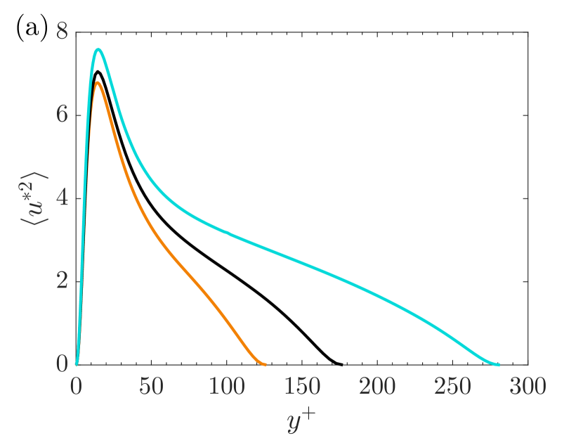
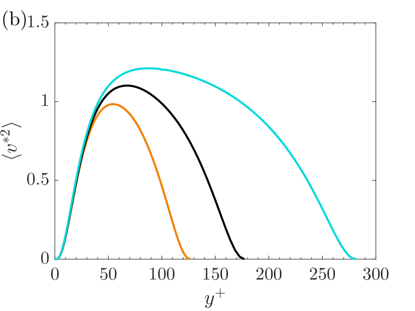
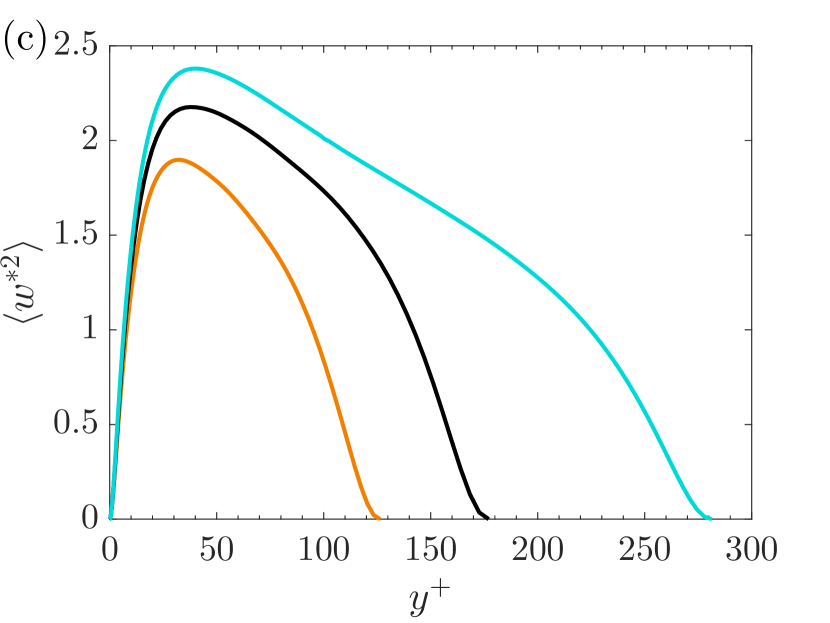
Figure 3: Turbulence intensities of the extracted small-scale near-wall fluctuating velocities at $Re_{\tau}=1000$, 2000 and 5200 using $y_{O}^{+}=3.9\sqrt{Re_{\tau}}$: (a) streamwise turbulence intensity, (b) wall-normal turbulence intensity and (c) spanwise turbulence intensity. Refer to table 1 for the line colors.

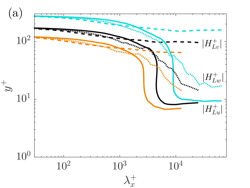
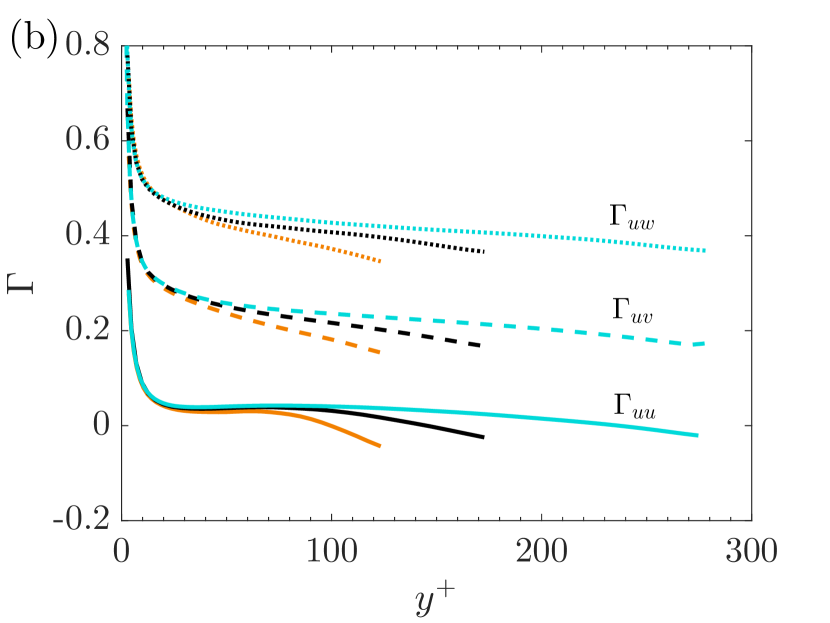
Figure 4: (a) Contour lines for the magnitudes of the scale-dependent kernel functions ($|H_{Lu}|$, $|H_{Lv}|$ and $|H_{Lw}|$) with a constant value of 0.6, and (b) profiles of the modulation coefficients ($\Gamma_{uu}$, $\Gamma_{uv}$ and $\Gamma_{uw}$) at $Re_{\tau}=1000,2000$ and 5200, where the solid lines represent $|H_{Lu}|$ and $\Gamma_{uu}$, dashed lines for $|H_{Lv}|$ and $\Gamma_{uv}$ and dotted lines for $|H_{Lw}|$ and $\Gamma_{uw}$, using $y_{O}^{+}=3.9\sqrt{Re_{\tau}}$, the vertical and spanwise modulation coefficients are moved up by 0.2 and 0.4, respectively. Refer to table 1 for the line colors.

Now we present application results of the extracting scheme (8 and 10) for the near-wall Reynolds-number-independent velocity fields. The primary input is the outer reference height $y_{O}^{+}$, since the kernel functions ($H_{Lu}$, $H_{Lv}$, $H_{Lw}$) and the imprint velocities ($u_{L}^{+}$, $v_{L}^{+}$, $w_{L}^{+}$) can be directly calculated once $y_{O}^{+}$ is given. In the majority of the previous studies, $y_{O}^{+}$ is chosen at the centre of the logarithmic layer [58, 93, 60], i.e. $y_{O}^{+}\approx 3.9\sqrt{Re_{\tau}}$, because the outer spectral peak of streamwise velocity fluctuations is located at this height [28]. As shown in FIG 3, we find that the extracted near-wall motions from the channel DNS data are actually Reynolds number dependent in the range of $Re_{\tau}=1000\sim 5200$. Additionally, the magnitudes of the footprint kernel functions ($H_{Lu}$, $H_{Lv}$ and $H_{Lw}$) and the amplitude modulation coefficients ($\Gamma_{uu}$, $\Gamma_{uv}$ and $\Gamma_{uw}$) are also Reynolds-number dependent, which is displayed in FIG 4. These results indicate that the near-wall influence from a portion of outer motions may be still included, if we trust the inner-outer interaction hypothesis and choose $y_{O}^{+}\approx 3.9\sqrt{Re_{\tau}}$. This could be true as Townsend [2] already proposed that the wall-attached eddies can influence the near-wall flow, and the geometrically self-similar eddies with sizes of $l_{y}^{+}<3.9\sqrt{Re_{\tau}}$ are probably active near the wall [3]. Therefore it suggests that the truly Reynolds-number-independent near-wall motions may be extracted by reducing the input reference height $y_{O}^{+}$. In addition, the small scale velocities $(u^{*},v^{*},w^{*})$ should be zero at $y^{+}=y^{+}_{O}$ according to the PIO model (see §3). Therefore, we stress that the optimal $y^{+}_{O}$ should be a constant in viscous scaling, since Reynolds number independence requires that the zero crossing height of $(u^{*},v^{*},w^{*})$ should be the same at different Reynolds numbers.

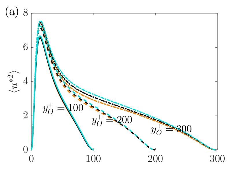
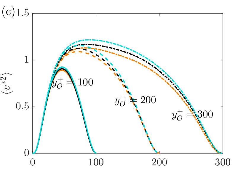
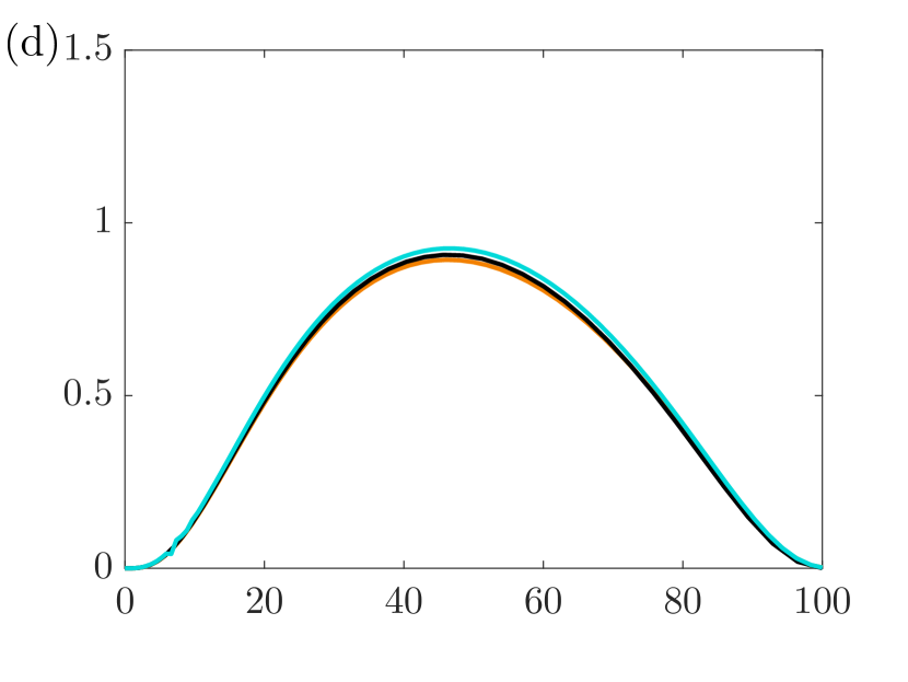
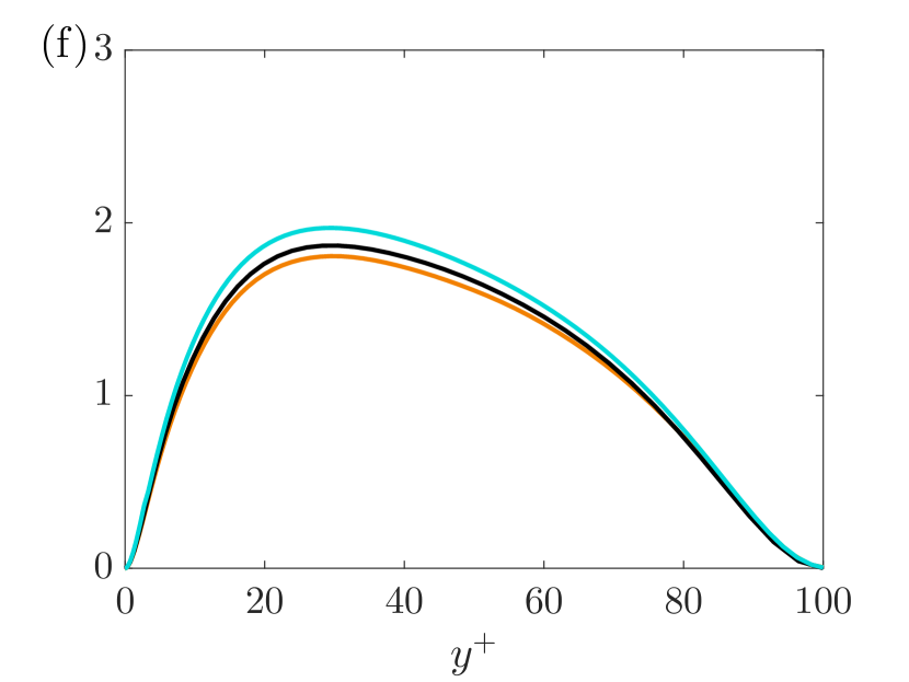
Figure 5: Turbulence intensities of the extracted Reynolds-number-independent fluctuating velocity components at $Re_{\tau}=$ 1000, 2000 and 5200: (a, b) streamwise velocity; (c, d) wall-normal velocity; (e, f) spanwise velocity. In (a, c, e), the reference wall-normal position $y_{O}^{+}$ varies from 300 to 100: $y_{O}^{+}=300$ (dot-dashed lines), $y_{O}^{+}=200$ (dashed lines) and $y_{O}^{+}=100$ (solid lines). In (b, d, f), only the results using the reference position $y_{O}^{+}=100$ are shown. Refer to table 1 for the line colors.

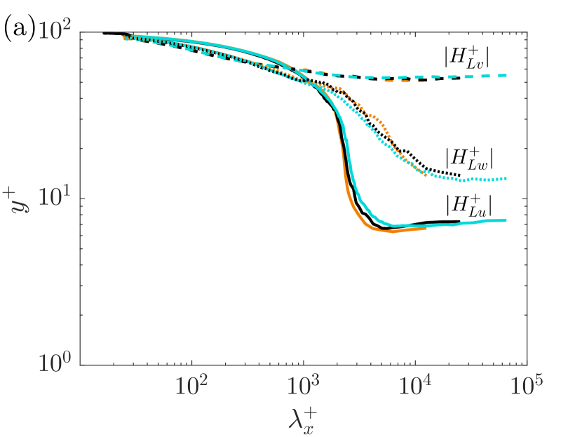
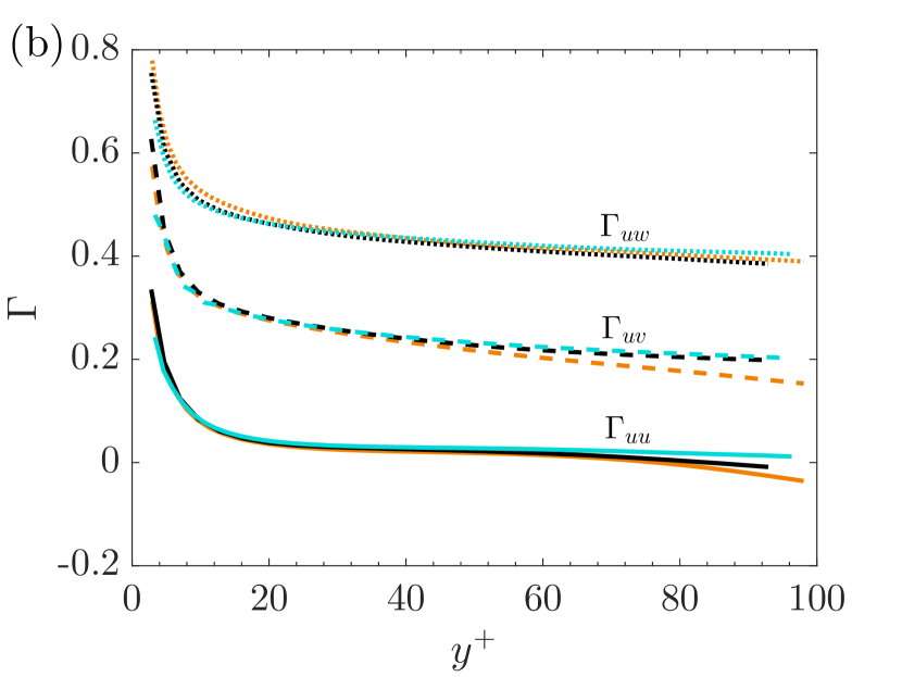
Figure 6: (a) Contour lines for the magnitudes of the scale-dependent kernel functions ($|H_{Lu}|$, $|H_{Lv}|$ and $|H_{Lw}|$) with a constant value of 0.6, and (b) profiles of the modulation coefficients ($\Gamma_{uu}$, $\Gamma_{uv}$ and $\Gamma_{uw}$) at $Re_{\tau}=1000,2000$ and 5200, where the solid lines represent $|H_{Lu}|$ and $\Gamma_{uu}$, dashed lines for $|H_{Lv}|$ and $\Gamma_{uv}$ and dotted lines for $|H_{Lw}|$ and $\Gamma_{uw}$, using $y_{O}^{+}=100$. And the vertical and spanwise modulation coefficients are moved up by 0.2 and 0.4, respectively. Refer to table 1 for the line colors.

By systematically decreasing the reference height $y_{O}^{+}$ from 300 to 200 and finally 100, it clearly shows that the extracted $\langle u^{*2}\rangle$, $\langle v^{*2}\rangle$, $\langle w^{*2}\rangle$ are less dependent on Reynolds number, if $y_{O}^{+}$ is smaller, as shown in FIG 5 (a, c, e). Furthermore, the Reynolds-number invariant $\langle u^{*2}\rangle$, $\langle v^{*2}\rangle$, $\langle w^{*2}\rangle$ could be well defined with $y_{O}^{+}=100$ and at $Re_{\tau}=1000\sim 5200$. In FIG 5 (b, d, f), only the extracted ($\langle u^{*2}\rangle$, $\langle v^{*2}\rangle$, $\langle w^{*2}\rangle$) with $y_{O}^{+}=100$ at the three Reynolds numbers are displayed and good collapse can be found. In addition, excellent Reynolds-number independence of the magnitudes of the footprint kernel functions ($H_{Lu}$, $H_{Lv}$ and $H_{Lw}$) and the amplitude modulation coefficients ($\Gamma_{uu}$, $\Gamma_{uv}$ and $\Gamma_{uw}$) are also obtained and demonstrated in FIG 6. The contour plots of $|H_{Lu}|$, $|H_{Lv}|$ and $|H_{Lw}|$ with $y^{+}_{O}=100$, 200 and 300 at $Re_{\tau}=1000\sim 5200$ are also presented in Appendix B. It should be noted that although $y_{O}^{+}=200$ and 300 are constants in viscous units, they actually locate in the logarithmic layer or outer layer. This is why $y^{+}_{O}=100$ works best, as it may be regarded as a critical height dividing the inner and outer regions.

Moreover, we present evidence of the extracted Reynolds-number-independent near-wall motions in the scale space through pre-multiplied streamwise and spanwise energy spectra of all the three velocity components at the Reynolds numbers $Re_{\tau}=1000\sim 5200$ with $y_{O}^{+}=100$, as shown in FIG 7. It is clearly seen that the spectra of the extracted $u^{*}$ and $v^{*}$ collapse excellently at the three Reynolds numbers. The inner peaks of the streamwise and spanwise $u^{*}$-spectra locate at $y^{+}=10\sim 20$, $\lambda_{x}^{+}\sim O(10^{3})$ and $\lambda_{z}^{+}\sim O(10^{2})$, which is well in accordance with experimental observations of near-wall streaks [72, 73, 74]. For the wall-normal components $v^{*}$, the spectral peaks locate at $y^{+}\approx 50$, $\lambda_{x}^{+}=200\sim 300$ and $\lambda_{z}^{+}\approx 100$. In accordance with the integrated spanwise velocity intensity $\langle w^{*2}\rangle$, it is also found there exists slight Reynolds number dependence in the pre-multiplied spectra of $w^{*}$, as displayed in FIG 7 (e, f). The discrepancy is principally located at large wavelengths, i.e., $\lambda_{x}^{+}>O(10^{3})$ and $\lambda_{z}^{+}>200\sim 300$. Here we claim that this discrepancy is only marginal and could be neglected. The spectral peaks of $w^{*}$ locate at similar wall-normal height and wavelengths with $v^{*}$, namely, $y^{+}=30\sim 40$, $\lambda_{x}^{+}=200\sim 300$ and $\lambda_{z}^{+}\approx 200$. Therefore, the wall-normal positions of ($v^{*}$, $w^{*}$) spectral peaks are much higher than that of $u^{*}$, while their streamwise and spanwise wavelengths are much smaller, which is consistent with the characteristics of the near-wall inner spectral peaks before decomposition (FIG 1). It is also noted that the $u^{*}$ and $w^{*}$ spectra can well penetrate into $y^{+}<10$ while the $v^{*}$ spectra are mainly located at $y^{+}>10$. This is due to the impermeable condition or the blocking effect of the wall-normal velocity at the wall [3, 94].

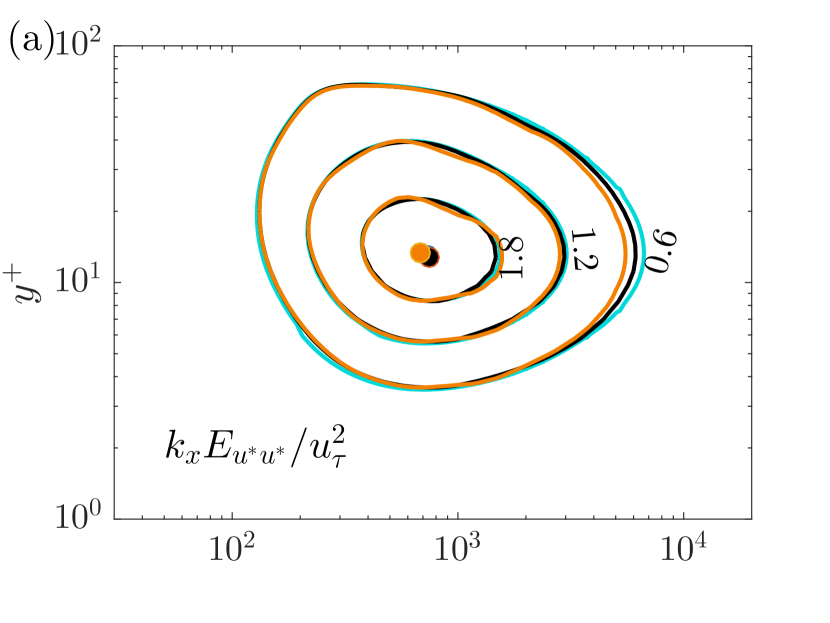
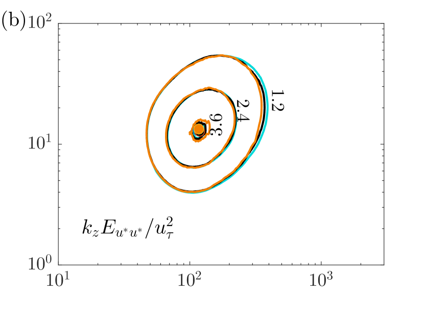
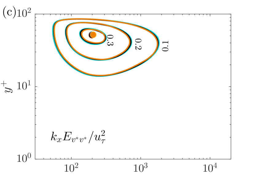
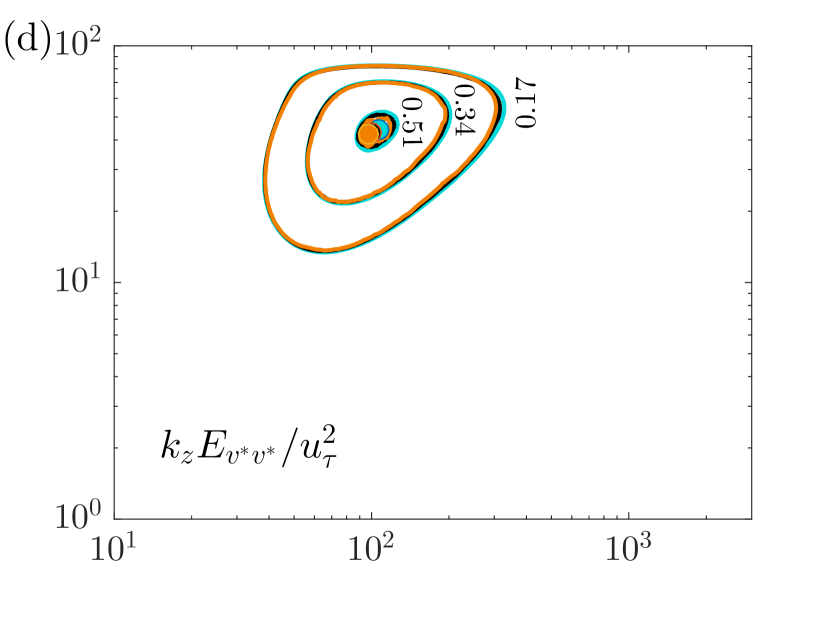
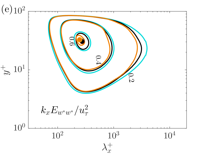
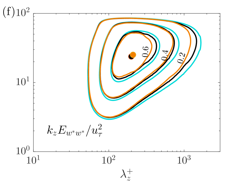
Figure 7: Pre-multiplied energy spectra of the three near-wall Reynolds-number-independent velocity components at $Re_{\tau}=1000$, 2000 and 5200. (a) $k_{x}E_{u^{*}u^{*}}/u_{\tau}^{2}$, (b) $k_{z}E_{u^{*}u^{*}}/u_{\tau}^{2}$, (c) $k_{x}E_{v^{*}v^{*}}/u_{\tau}^{2}$, (d) $k_{z}E_{v^{*}v^{*}}/u_{\tau}^{2}$, (e) $k_{x}E_{w^{*}w^{*}}/u_{\tau}^{2}$ and (f) $k_{z}E_{w^{*}w^{*}}/u_{\tau}^{2}$. The locations of spectral peaks have been marked with symbols. Refer to table 1 for the line colors.

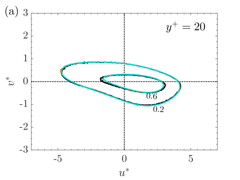
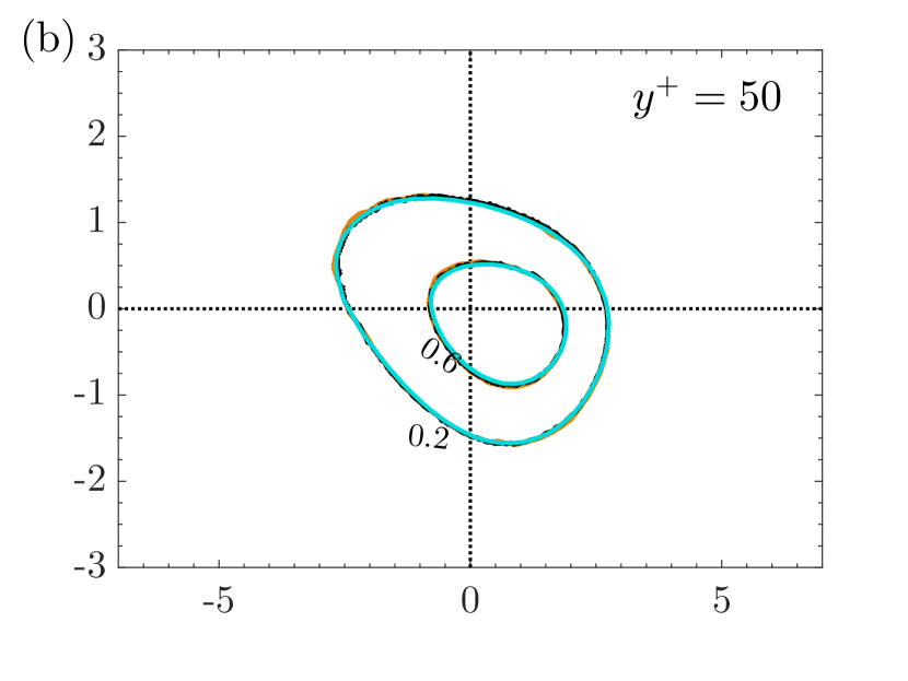
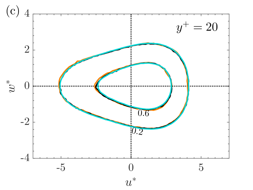
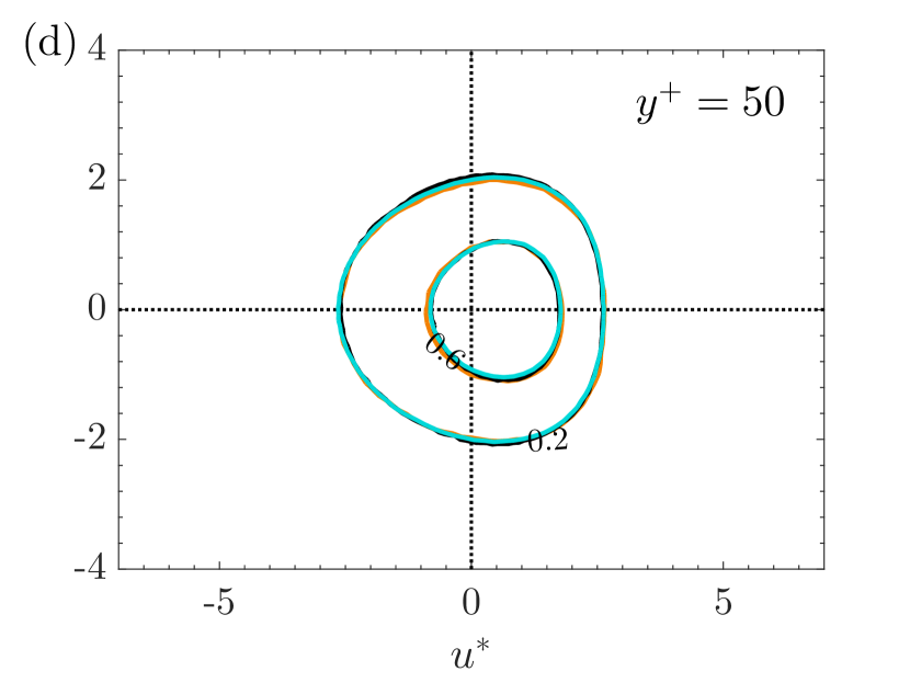
Figure 8: Joint p.d.f.s $P(u^{*},v^{*})$) (a, b) and $P(u^{*},w^{*})$ (c, d) at $y^{+}$ = 20 (a, c) and $y^{+}$ = 50 (b, d) in the fully developed turbulent channel flows at the Reynolds numbers $Re_{\tau}=1000\sim 5200$. The contour levels are normalized by the peak value of the p.d.f. at $Re_{\tau}=1000$ of the two heights. Refer to table 1 for the line colors.

Furthermore, we present joint p.d.f.s $P(u^{*},v^{*})$ and $P(u^{*},w^{*})$ of the extracted near-wall Reynolds-number-independent velocities at the Reynolds number $Re_{\tau}=1000\sim 5200$, which is displayed in FIG 8. The comparisons at the two wall-normal heights $y^{+}=20$ and $y^{+}=50$ exhibit remarkable coincidence of the joint p.d.f.s of the extracted Reynolds-number-independent velocity components at the three Reynolds numbers. The major axis of $P(u^{*},v^{*})$ is inclined in the Q2-Q4 direction, indicating higher probabilities of the ejection and sweep motions. By comparing $P(u^{*},v^{*})$ at the two heights, i.e. FIG 8 (a) and (b), it can be seen that the inclination of the major axis is shallower at $y^{+}=20$, suggesting the ejecting or sweeping of the turbulent motions occurs at a smaller angle nearer the wall, similar to FIG 2 (a, b). In addition, the joint p.d.f. $P(u^{*},w^{*})$ is shown in FIG 8 (c, d), which is symmetric about $w^{*}=0$ axis, also similar to FIG 2 (c, d).

So far, Reynolds-number-invariant statistics of the decomposed small-scale near-wall motions have been thoroughly demonstrated, in the Reynolds number range of $Re_{\tau}=1000\sim 5200$. Now we turn to demonstrate the corresponding instantaneous flow snapshots and reveal the dominant coherent structures composing the Reynolds-number-independent near-wall flow. FIG 9 displays $x-z$ plane snapshots of the Reynolds-number-independent streamwise velocity at $y^{+}=15$, where the full streamwise velocity fluctuation intensity is approximately the maximum. It is seen that, as Reynolds number increases (i.e., FIG 9 (a,c,e)), the general streaky features of the flows are quite similar, indicating that not only the statistics, but also the instantaneous fields of $u^{*}$ exhibit good Reynolds-number-independent behavior. Furthermore, instantaneous $w^{*}$ fields are shown on FIG 9 (b,d,f) at the $y^{+}=25$, which shows that there is no evident residual large-scale footprints.

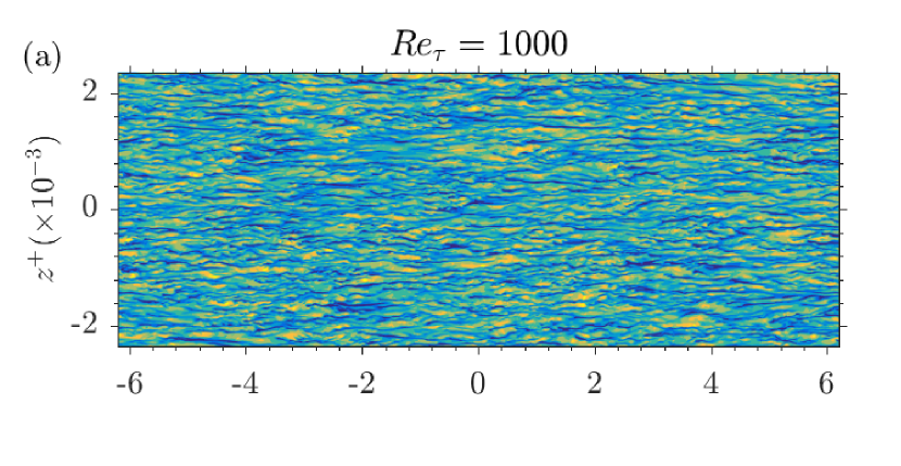
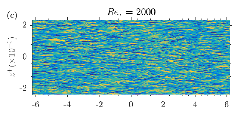
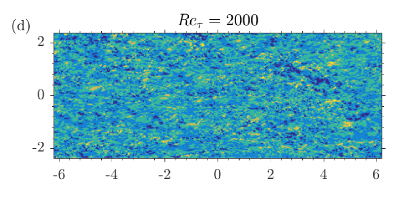
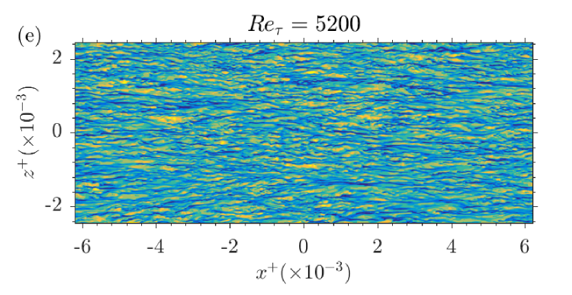
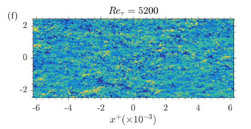
Figure 9: Plane snapshots of the near-wall Reynolds-number-independent streamwise velocity fields at $y^{+}=15$ (a,c,e) and Reynolds-number-independent spanwise velocity fields at $y^{+}=25$ (b,d,f) for $Re_{\tau}=1000,2000,5200$.

In FIG 10, we show Reynolds-number invariance of vortical statistics of the Reynolds-number-independent flow fields. The $\lambda_{ci}$ criterion [95] is employed for the vortex identification, which is defined as the imaginary part of the complex eigenvalue of velocity gradient tensor and usually referred to the local swirling strength. The p.d.f.s of $\lambda_{ci,*}$ at the three Reynolds numbers, i.e., $Re_{\tau}=1000,2000$ and 5200, are plotted in FIG 10 (a), which demonstrates excellent agreement among the three distributions. Meanwhile, the wall-normal variation of the most probable value of $\lambda_{ci,*}$ is represented by the black dotted line, the maximum of which is located around $y^{+}=25$. Furthermore, FIG 10 (b) exhibits the mean swirling strength profiles. It is seen that, the mean swirling strength increases first and then decreases with $y^{+}$, and the maximum also appears at $y^{+}=25$. Excellent Reynolds-number invariance is observed. An approximately linear variation of the mean swirling strength $\langle\lambda_{ci,*}\rangle$ with $y^{+}$ in the range of $y^{+}\approx 30\sim 75$ is also denoted in the FIG 1. Since the swirling strength is defined in terms of velocity gradient, it is of higher order than velocity itself, and the comparison here further strengthens the reliability of the current extraction scheme for the Reynolds-number-independent velocity field.

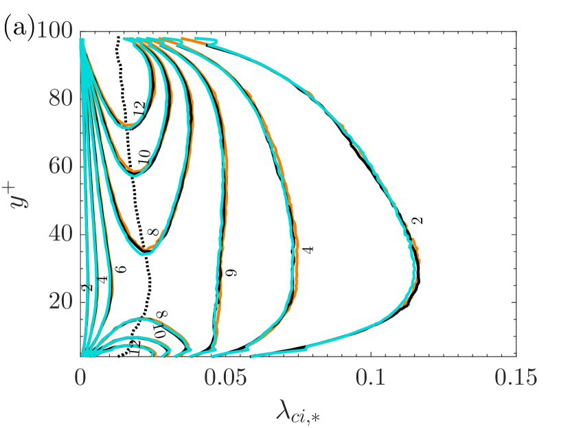
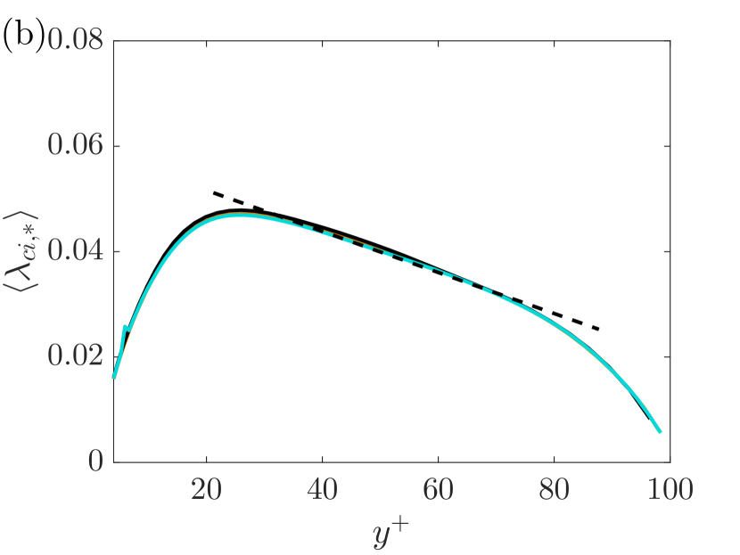
Figure 10: P.d.f.s of $\lambda_{ci,*}$ (a) and mean swirling strength $\langle\lambda_{ci,*}\rangle$ (b) as functions of $y^{+}$ at $Re_{\tau}=1000$, 2000 and 5200. The dashed line indicates a linear variation of $\langle\lambda_{ci,*}\rangle$ with $y^{+}$. Refer to table 1 for the line colors.

Besides swirling strength $\lambda_{ci}$, vortex orientation is another important aspect for the characterization of vortical structures. Zhou et al. [95] suggested that local swirling flow will be stretched or compressed along the direction of the real eigenvector $\mathbf{\Lambda}_{r}$ of the velocity gradient tensor. Gao et al. [96] employed $\mathbf{\Lambda}_{r}$ to identify the local vortex orientations. Recently, Wang et al. [97] analyzed the vortex geometries and topologies in turbulent boundary layers measured by tomographic particle image velocimetry using the same method. Following the above studies, in this work, we also identify the vortex orientations through the real eigenvector $\Lambda_{r}$ of the velocity gradient tensor. For the details of the method, one could see Gao et al. [96] and Wang et al. [97]. FIG 11 illustrates the p.d.f.s of the vortex orientations at $Re_{\tau}=1000\sim 5200$, where the $\Lambda_{r}$ vector is projected onto the $x-y$ plane and $x-z$ plane separately. In the $x-y$ plane, the angle between the projected vector and the $x$ axis is denoted by $\theta_{xy}$. In the $x-z$ plane, the angle between the projected $\Lambda_{r}$ vector and the negative $z$ axis is indicated by $\theta_{-zx}$. FIG 11 clearly shows that the p.d.f.s collapse excellently, i.e., demonstrating Reynolds number invariance of vortex orientations. Wang et al. [97] reported that the near-wall vortex orientations from the full velocity fields are also nearly independent of Reynolds number in the range of $Re_{\tau}=1238\sim 3081$. They attributed it to that the Reynolds number only has evident influence on large-scale flow structures, while the small-scale vortical structures are likely independent of the Reynolds number.

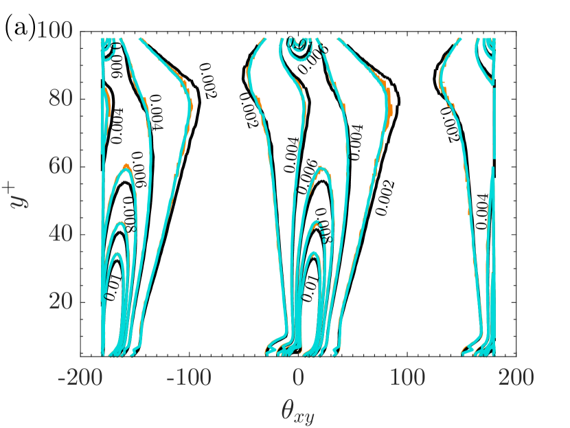
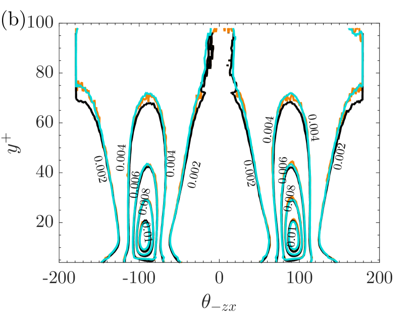
Figure 11: P.d.f.s of $\theta_{xy,*}$ (a) and $\theta_{-zx,*}$ (b) as functions of $y^{+}$ at $Re_{\tau}=1000$, 2000 and 5200. Refer to table 1 for the line colors.

In summary, here we have successfully demonstrated that truly Reynolds-number-independent near-wall turbulent motions that are independent of outer influences have been successfully extracted via the inner-outer interaction hypothesis, the extraction scheme (8-10) and the outer reference height $y_{O}^{+}=100$, in the Reynolds number range of $Re_{\tau}=1000\sim 5200$. Plenty of evidence, i.e., integrated statistics, spectra, joint p.d.f. as well as instantaneous flow fields, has been provided.

V Low-Reynolds-number effect

Some studies have reported the existence of the low-Reynolds-number effect ($180<Re_{\tau}<1000$), that near-wall turbulence statistics can not be well scaled by the viscous units at low Reynolds numbers [20, 22, 23]. It is unclear whether this anomalous scaling is due to the effect of outer footprints, which should not be very strong at low Reynolds number in our view. In this part, we will inspect whether the small-scale near-wall velocity fields extracted by (8-10) could also be Reynolds-number-independent in the fully developed low-Reynolds-number turbulent channel flows, e.g., $Re_{\tau}<1000$.

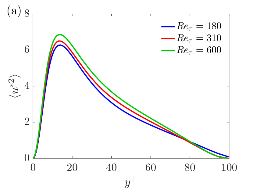
Figure 12: The intensities of the extracted $u^{*}$ (a), $v^{*}$ (b) and $w^{*}$ (c) at $Re_{\tau}=180,310$ and 600. Refer to table 1 for the line colors.

The intensities of the extracted $u^{*}$, $v^{*}$ and $w^{*}$ in the context of the inner-outer interaction model are shown in FIG 12. It is seen that the streamwise turbulence intensity $\langle u^{*2}\rangle$ slightly increases with $Re_{\tau}$ and the intensity peaks locate at $y^{+}\approx 15$ at all the three Reynolds numbers, as displayed in FIG 12 (a). The Reynolds number dependence is also evident from the wall-normal and spanwise turbulence intensities, i.e., $\langle v^{*2}\rangle$ and $\langle w^{*2}\rangle$, as shown in FIG 12 (b) and (c). The wall-normal peak locations of $\langle v^{*2}\rangle$ and $\langle w^{*2}\rangle$ are $y^{+}\approx 40\sim 50$ and $y^{+}\approx 30\sim 40$, respectively. Therefore, the extracted $\langle u^{*2}\rangle$, $\langle v^{*2}\rangle$ and $\langle w^{*2}\rangle$ are not Reynolds-number-independent, instead they show definite Reynolds number dependence. Then, we will denote it as low Reynolds number effect hereafter, which should not be confounded with that in the literature [22, 23], since the large scales were present and small scales were not separated from the total fluctuations. In addition, we also tried smaller $y_{o}^{+}$ at these low Reynolds numbers, and the results are presented in Appendix C. It is found that the low-Reynolds-number effect still exists.

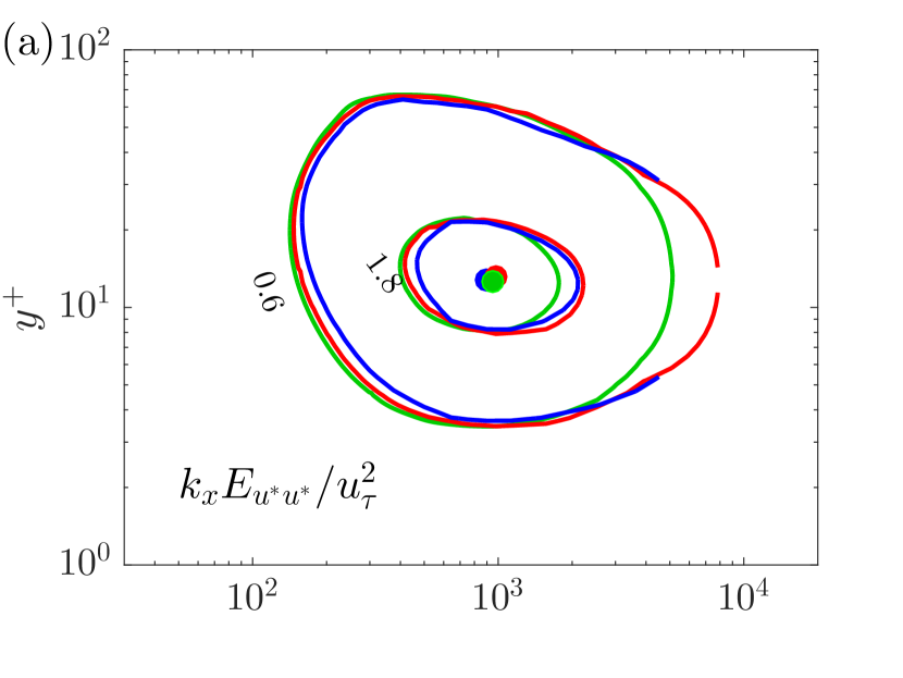
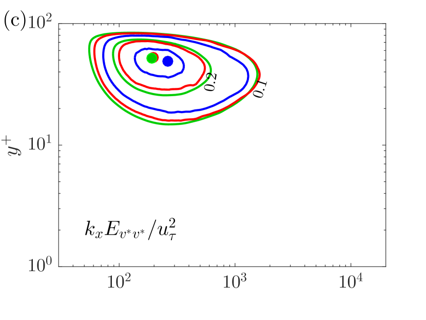
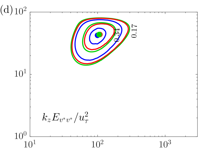
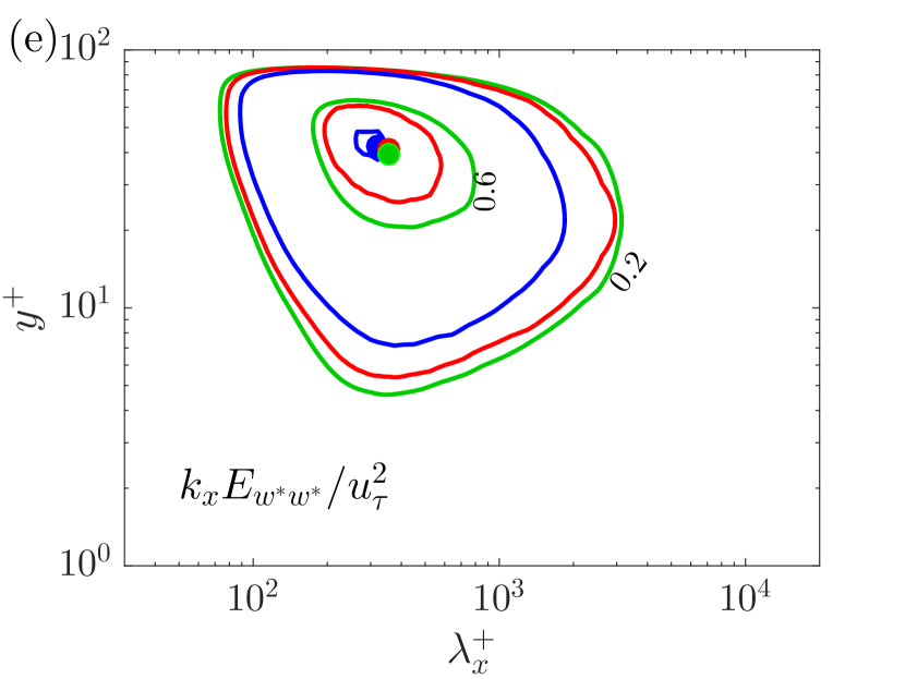
Figure 13: Pre-multiplied energy spectra of the three near-wall small-scale velocity components at $Re_{\tau}=$180, 310 and 600. (a) $k_{x}E_{u^{*}u^{*}}/u_{\tau}^{2}$, (b) $k_{z}E_{u^{*}u^{*}}/u_{\tau}^{2}$, (c) $k_{x}E_{v^{*}v^{*}}/u_{\tau}^{2}$, (d) $k_{z}E_{v^{*}v^{*}}/u_{\tau}^{2}$, (e) $k_{x}E_{w^{*}w^{*}}/u_{\tau}^{2}$ and (f) $k_{z}E_{w^{*}w^{*}}/u_{\tau}^{2}$. The locations of spectral peaks have been marked with symbols. Refer to table 1 for the line colors.

Furthermore, similar to FIG 13, we show the one-dimensional streamwise and spanwise pre-multiplied energy spectra of the three small-scale velocity components at the low Reynolds numbers in FIG 13, with the viscous-scaled wavelength ($\lambda_{x}^{+}$ or $\lambda_{z}^{+}$) and the wall-normal height $(y^{+})$. For the contour level, we try to keep consistent with FIG 13, but for clarity, only two levels between zero and the peak values are shown. As displayed in FIG 13 (a,b), the near-wall spectral peaks of the streamwise and spanwise pre-multiplied spectra locate at $y^{+}=10\sim 20$ with $\lambda_{x}^{+}\sim O(10^{3})$ and $\lambda_{z}^{+}\sim O(10^{2})$, which are similar with those in FIG 1 and FIG 13. However, it may not be claimed with confidence that the spectral contours are perfectly scaled by viscous units. In fact, FIG 13 (a) shows that the streamwise wavelength of the inner peak is slightly larger at lower Reynolds numbers, which is consistent with our previous simulations at much lower Reynolds numbers [70]. Meanwhile, the spanwise wavelength of the inner peak is larger at higher Reynolds number, see FIG 13 (b). This may indicate that as Reynolds number increases, the near-wall small-scale $u^{*}$ structures tend to be shorter and wider, in the low Reynolds number regime. Moreover, in FIG 13 (c-f), the streamwise and spanwise pre-multiplied energy spectra of $v^{*}$ and $w^{*}$ are presented, in which the wall-normal locations of the inner spectral peaks are also consistent with the undecomposed ones, as in FIG 1 (c-f), say $y^{+}=30\sim 70$. Compared to the $u^{*}$-spectra, the $v^{*}$- and $w^{*}$-spectra exhibit much stronger Reynolds number dependence. Particularly, as Reynolds number increases, the spectral energy increases accordingly, resulting in stronger integrated $\langle v^{*2}\rangle$ and $\langle w^{*2}\rangle$, as shown in FIG 12 (b) and (c). Since the spanwise and wall-normal velocity components are closely related to vortical structures, it may imply that the strength of near-wall small-scale quasi-streamwise vortices increases with Reynolds number in the low $Re_{\tau}$ regime ($Re_{\tau}<1000$), and can reach a fully-developed asymptotic status once $Re_{\tau}\geq 1000$. It should be mentioned that Antonia & Kim [23] also attributed the low-Reynolds-number effect to an increase in strength of the quasi-streamwise vortices in the buffer layer, other than the average diameter or average location.

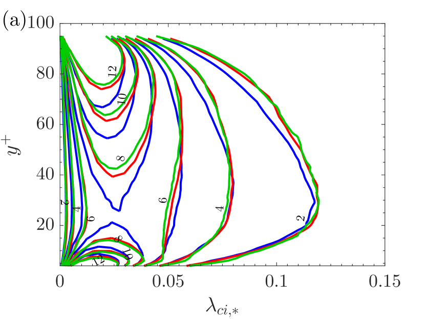
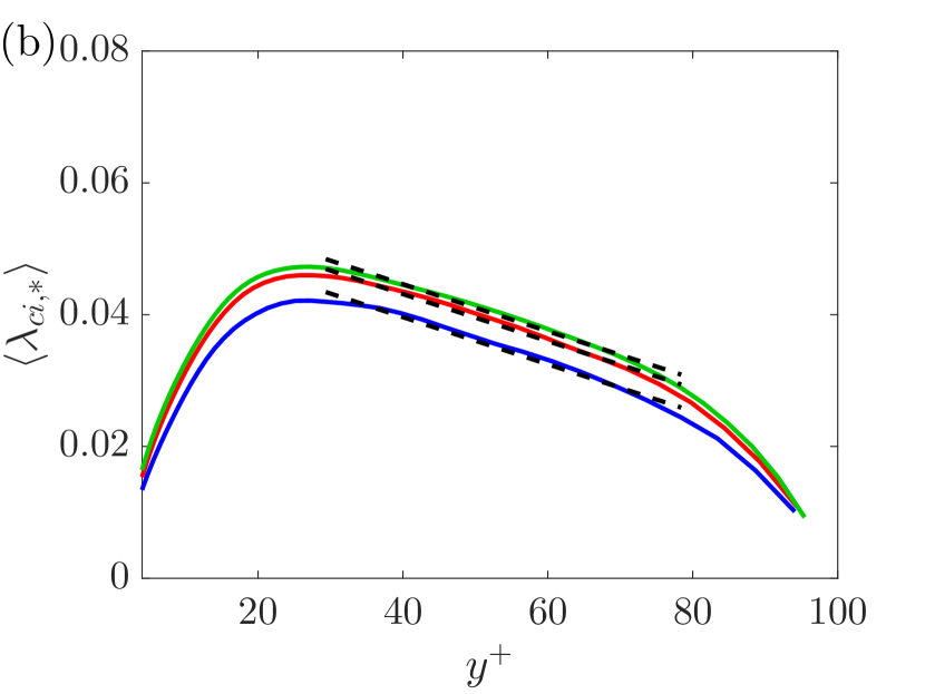
Figure 14: P.d.f.s of $\lambda_{ci,*}$ (a) and mean swirling strength $\langle\lambda_{ci,*}\rangle$ (b) as functions of $y^{+}$ at $Re_{\tau}$ = 180, 310 and 600. Refer to table 1 for the line colors.

Finally, we illustrate the low-Reynolds-number effect on the swirling strength statistics. The p.d.f. distributions of $\lambda_{ci,*}$ at $Re_{\tau}=180$, 310 and 600 in the near-wall region are compared in FIG 14 (a). The shapes of the p.d.f.s at the different Reynolds numbers are generally similar. However, it can be clearly seen that, as Reynolds number increases, the probability of large swirling strength gradually becomes higher, indicating stronger vortical strength at higher $Re_{\tau}$. Besides, FIG 14 (b) demonstrates the mean swirling strength profiles at the three low Reynolds numbers. The swirling strength increases first then decreases with $y^{+}$, and the maximum value appears at $y^{+}\approx 25$, which is similar to the higher Reynolds number cases, as in FIG 10 (b). However, the absolute value of $\lambda_{ci,*}$ is found to increase with $Re_{\tau}$ and be consistent with the p.d.f. result. Moreover, the linear relationship also exists and almost has an identical slope from $Re_{\tau}=$180 to 5200 in the range of $y^{+}=30\sim 75$. In addition, the mean inclination and the corresponding p.d.f. of the near-wall small-scale vortex structures are found to be basically independent of Reynolds number, which are not shown here for saving space.

In summary, we have applied the decomposition scheme (8-10) to the low-Reynolds-number turbulent channels at $Re_{\tau}=180\sim 600$, and the extracted near-wall small-scale velocity fields ($u^{*}$, $v^{*}$ and $w^{*}$) are discovered to be Reynolds number dependent. The main mechanism may be the strengthening of the near-wall quasi-streamwise vortical structures. And it will induce the augments of the velocity fluctuations, as well as the widening and shortening of the near-wall streaks.

VI Characteristics of outer footprints

In this part, we present the characteristics of the near-wall footprints of outer turbulent motions, i.e., $(u_{L},v_{L},w_{L})$, also known as the superposition effect [40, 59, 58], as well as their interactions with the near-wall small-scale motions, which is quantified by the amplitude modulation of large scales to small scales.

We scrutinize the spectral energy distributions of the outer footprints in the near-wall region. The streamwise and spanwise pre-multiplied energy spectra of all the three velocity components with the viscous scaling, are given in FIG 15. In FIG 15 (a) and (b), it is shown that the TKE spectral distribution of $u_{L}$ seems to obey the viscous scaling very well in the range of $\lambda_{x}^{+}<6000$ and $\lambda_{z}^{+}<500$ approximately at $Re_{\tau}\geq 1000$. Furthermore, the pre-multiplied energy spectra of the wall-normal velocity footprints $v_{L}$ are displayed in FIG 15 (c,d). It is seen that excellent collapse is found with the viscous scaling with $\lambda_{x}^{+}<1000$ and $\lambda_{z}^{+}<300$ at $Re_{\tau}\leq 1000$. The pre-multiplied spectra of the spanwise velocity footprints $w_{L}$ are shown in FIG 15 (e,f). In the wavelength region of $\lambda_{x}^{+}\leq 600$ and $\lambda_{z}^{+}<400$ at $Re_{\tau}\leq 1000$, it can be clearly seen that the spectra are well collapsed with the viscous-scaled wavelength.

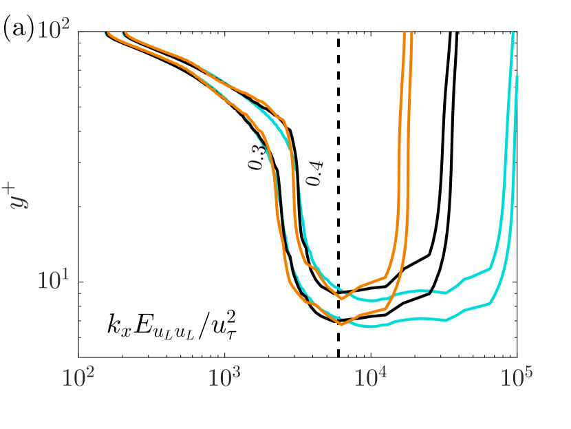
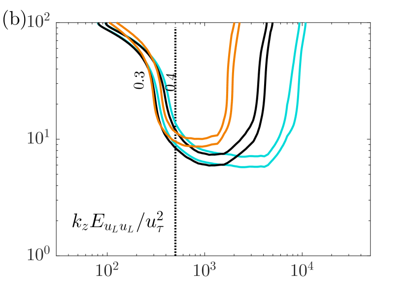
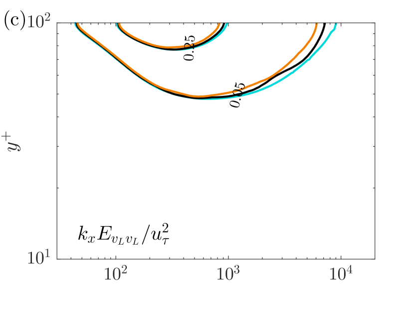
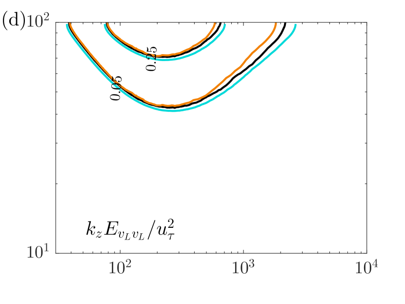
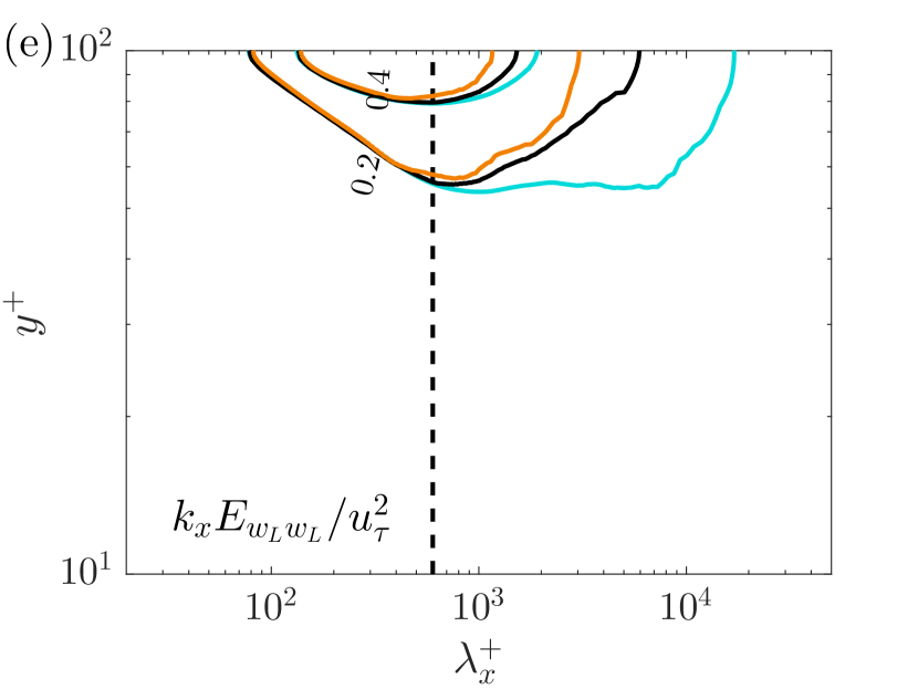
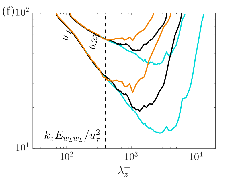
Figure 15: Streamwise (a,c,e) and spanwise (b,d,f) pre-multiplied energy spectra of the outer footprint velocity components $(u_{L},v_{L},w_{L})$ with the viscous-scaled wavelength $\lambda_{x}^{+}$ and $\lambda_{z}^{+}$. Refer to table 1 for the line colors.

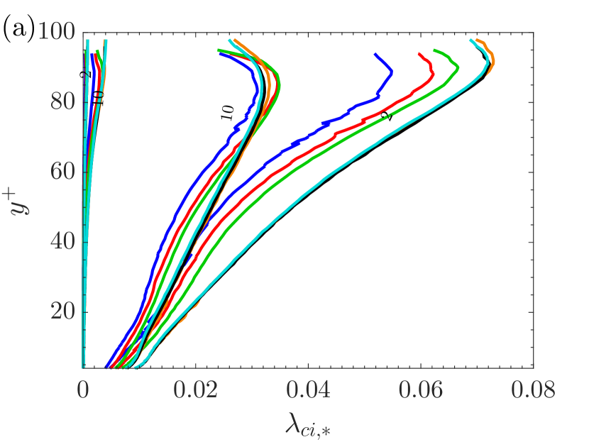
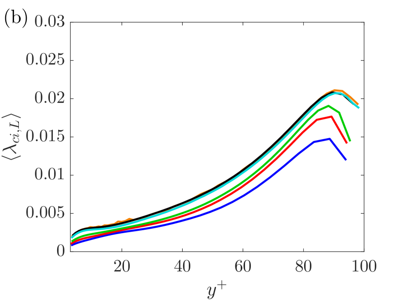
Figure 16: P.d.f.s (a) and mean profiles (b) of $\lambda_{ci,L}$ as functions of $y^{+}$ at the Reynolds numbers from 180 to 5200. Refer to table 1 for the line colors.

At last, we demonstrate the Reynolds-number effect on the swirling strength statistics of outer footprint fields. The p.d.f. distributions of $\lambda_{ci,L}$ at the Reynolds numbers from 180 to 5200 in the near-wall region are compared in FIG 16 (a). The contours of the p.d.f.s exhibit excellent collapse at the Reynolds numbers of 1000, 2000 and 5200. However, the swirling strengths at lower Reynolds numbers show definite $Re_{\tau}$ dependence, and decreases as Reynolds number decreases. FIG 16 (b) displays the mean swirling strength profiles at different Reynolds numbers. It can be seen that, the mean swirling strength $\langle\lambda_{ci,L}\rangle$ is generally larger at higher $y^{+}$, while only decays at about $y^{+}>90$ possibly due to the decrease of the gradient of $u_{i,L}$ near $y^{+}=100$. At the three higher Reynolds numbers, i.e., $Re_{\tau}=1000$, 2000 and 5200, the $\langle\lambda_{ci,L}\rangle$ profiles collapse very well which is consistent with FIG 16 (a), but not the case at lower Reynolds numbers which is increasing with the Reynolds number.

VII Concluding remarks

In this work, we present a scaling based decomposition methodology of three-dimensional turbulence velocities into small-scale and large-scale components in the near-wall region at $y^{+}<100$. The method is principally based on the refined PIO model of Baars et al. [60]. However, a significant difference is that we use $y_{O}^{+}=100$ instead of $y^{+}_{O}=3.9\sqrt{Re_{\tau}}$ as the reference height for evaluating outer footprints. Reynolds-number-invariant small-scale turbulent motions are then extracted at $1000\leq Re_{\tau}\leq 5200$ with plenty of evidences, including integrated intensities, spectra and joint p.d.f.s of velocity fluctuations, as well as vortex swirling quantities. Finally, it is discovered that a small-scale part of the outer footprint can also be well scaled by the viscous units, as well as the vortical statistics.

The reason for the improved scaling collapse can be simply attributed to that the eddies with size of $100<l_{y}^{+}<3.9\sqrt{Re_{\tau}}$ should also be responsible and incorporated for near-wall footprints, and $y^{+}\approx 100$ can be regarded as one ’critical’ dividing height of inner and outer regions in the context of inner-outer interactions. A recent experimental investigation in open channel flows also supports it [98]. This can be further elucidated by the properties of attached eddies and detached eddies [99, 100, 101] that both have coherence with the wall. The detached eddies in the context of Hu et al. [101] are longer than the attached eddies and peaked at the centre of the logarithmic layer approximately. This is why previous studies commonly used $y^{+}_{O}=3.9\sqrt{Re_{\tau}}$, where the outer spectral peak resides [58, 60]. However, the attached eddies are more populated near the wall and lead to the logarithmic decay of $\langle u^{+2}\rangle$. As illustrated in FIG 17, if we use $y^{+}_{O}\sim\sqrt{Re_{\tau}}$, only the contribution of the largest attached eddies is included. In order to take into account smaller eddies, it is required to let $y^{+}_{O}=l_{y1}^{+}$, i.e., the size of the smallest attached eddies. According to the present finding, it is suggested that $l_{y1}^{+}=y^{+}_{O}\approx 100$, which is consistent with previous conjecture that the smallest attached eddies should be on the order of 100 viscous units in height [3].

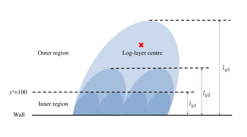
Figure 17: Sketch of a hierarchical structure of attached eddies with three levels.

At lower Reynolds numbers of $Re_{\tau}<1000$, we find that the extracted small-scale velocity and swirling-strength statistics can not be scaled by the viscous units. The intensities of these turbulence quantities increase with Reynolds number, showing a developing trend of near-wall small-scale turbulence. After examining the vortical structures, it is revealed that the overall swirling strength of the small-scale motions is enhanced at larger $Re_{\tau}$, which is consistent with the vortex strengthening mechanism [20, 22, 23].

The Reynolds-number independence of the extracted small-scale motions is not obtained at low Reynolds numbers, thus we may add a restriction for applications of the PIO model as $Re_{\tau}\geq 1000$. On the other hand, the low-Reynolds-number effect could probably not be a surprise, which can also be observed in FIG 1 before decomposition, and explained by insufficient separation of inner and outer scales in this range. Another related issue is the quasi-steady-quasi-homogeneous (QSQH) theory proposed by Chernyshenko and coworkers [102, 103], in which it is assumed that the small-scale motions vary much faster than the large-scale motions, therefore should be universal if scaled by local large-scale wall shear stress, instead of the mean one in the viscous scaling. Moreover, some studies [104, 105] also showed that velocity fluctuations can be better-scaled accounting by the effect of the mean shear. In fact, the QSQH theory admits two universalities, i.e., one is Reynolds-number invariance as in the PIO model, and the other is the independence of the small scales scaled by the large-scale wall shear stress. The former one was validated by Chernyshenko and coworkers using spectral cut-off filters [106, 107].The latter has been recently checked by Agostini & Leschziner [108] at a single Reynolds number of $Re_{\tau}\approx 1000$. Each one of the two universalities may not rely on the other. Whether the low-Reynolds-number data satisfies the second universality of the QSQH theory or not could be checked in future.

Availability of data

The data that support the findings of this study are available from the corresponding author upon reasonable request.

Appendix A Validation of the present DNS data

The low-Reynolds-number data are generated by our own DNS and here compared with the DNS data of [32] at similar Reynolds numbers to validate the present data quality. The fluctuating intensities of all three velocity components and the Reynolds shear stress are shown in FIG 18, where the present results at $Re_{\tau}$ = 180 and 600 are compared with the data of [32] at $Re_{\tau}$ = 180 and 550, respectively. FIG 18 confirms the excellent agreements between the two simulations, verifying the adequacy of the present DNS data. It is also noted that the slightly larger $\langle u^{+2}\rangle$ of the present DNS in (b) is probably due to the higher Reynolds number.

Figure 18: Comparison of the turbulence intensities ($\langle u^{2},v^{2},w^{2}\rangle^{+}$) and Reynolds shear stress $\langle uv\rangle^{+}$ between the present DNS and [32] (indicated by LM15) at $Re_{\tau}$ = 180 (a) and $Re_{\tau}$ = 600 (b). The LM15 data in (b) is at $Re_{\tau}$ = 550.

Appendix B Characteristics of $H_{Lu}$, $H_{Lv}$ and $H_{Lw}$ with different $y^{+}_{O}$

Here the contour plots of $|H_{Lu}|$, $|H_{Lv}|$ and $|H_{Lw}|$ with $y^{+}_{O}=100$, 200 and 300 at $Re_{\tau}=1000\sim 5200$ are compared in FIG 19. It can clearly seen that the contour lines of different Reynolds numbers are not well collapsed at large scales with $y^{+}_{O}=200$ and 300, while much improved collapse can be found with $y^{+}_{O}=100$.

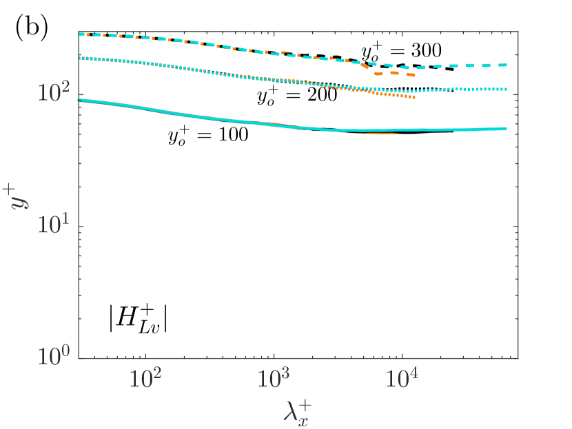
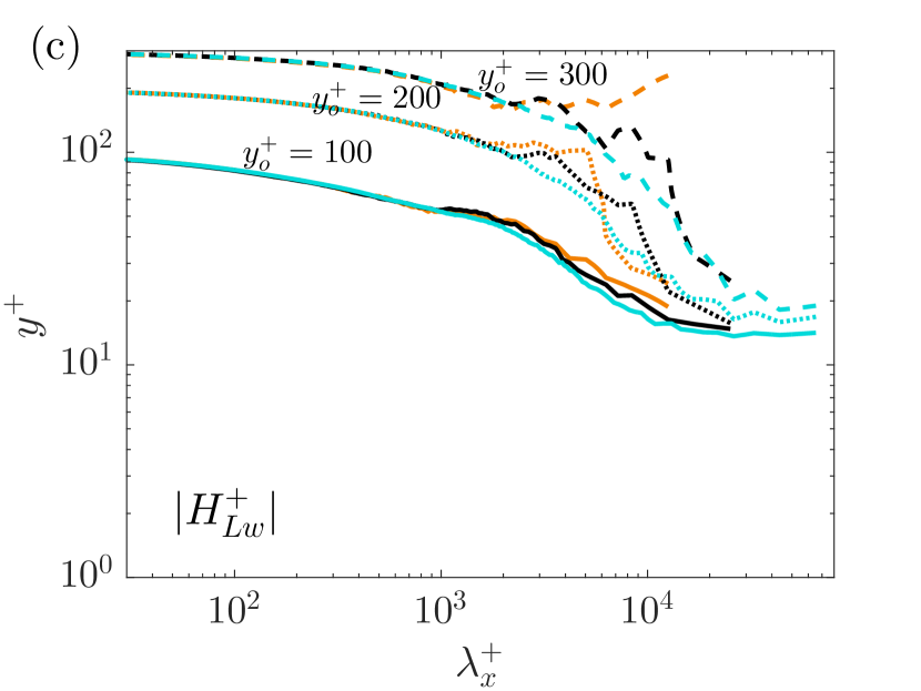
Figure 19: Contour lines for the magnitudes of the scale-dependent complex-valued kernel functions, (a) $|H_{Lu}|$, (b) $|H_{Lv}|$ and (c) $|H_{Lw}|$ with a constant value of 0.6, and solid lines for $y_{O}^{+}=100$, dotted lines for $y_{O}^{+}=200$, dashed lines for $y_{O}^{+}=300$. Refer to table 1 for the line colors.

Appendix C Effect of the outer reference height $y^{+}_{O}$ at low Reynolds numbers

We have shown that excellent viscous scaling of $u^{*}$, $v^{*}$ and $w^{*}$ can be obtained with $y^{+}_{O}=100$ at $Re_{\tau}=1000\sim 5200$, while low-Reynolds-number effect exists at $Re_{\tau}=180\sim 600$ using the same $y_{O}^{+}$. It may be argued that $y^{+}=100$ is located in the outer region at the low Reynolds numbers with the outer scaling ($\delta$ and $u_{\tau}$). Therefore it may be interesting to see what will happen if further lowering $y^{+}_{O}$ at the low Reynolds numbers. FIG 20 shows the intensities of the extracted $u^{*}$, $v^{*}$ and $w^{*}$ at the low Reynolds numbers from 180 to 600, with $y^{+}_{O}$ = 60. It is seen that the scaling of $u^{*}$ is improved slightly, compared to FIG 12 (a), while the low-Reynolds-number effect still exists for $v^{*}$ and $w^{*}$. Therefore, it may indicate that using smaller $y_{O}^{+}$ can not relieve the anomalous scaling, and the low-Reynolds-number effect may be an objective phenomenon.

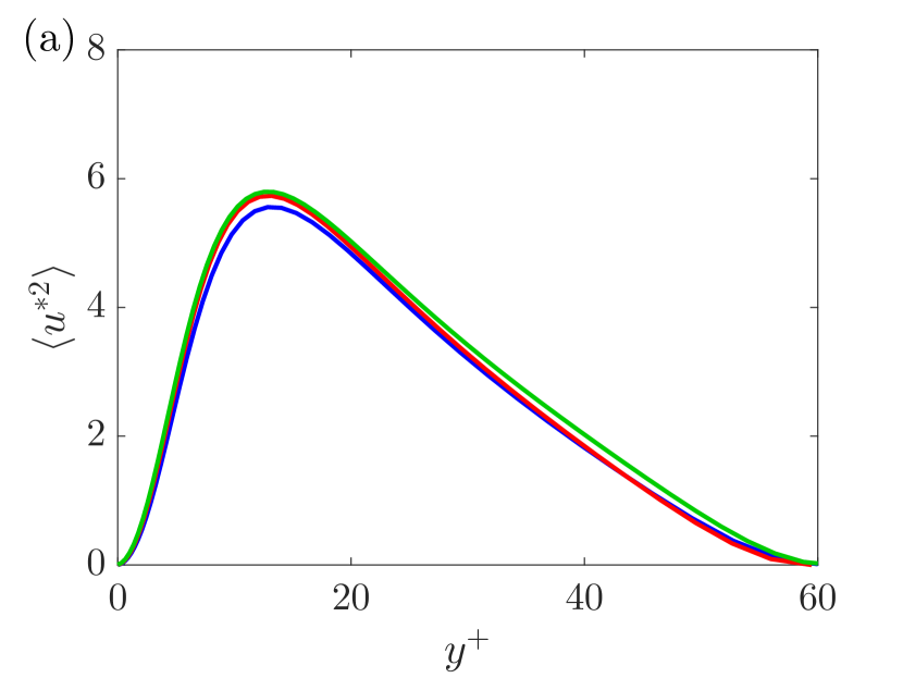
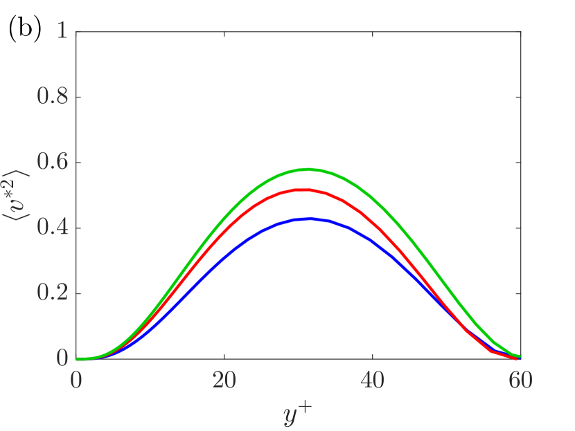
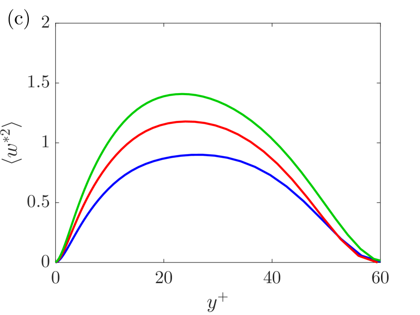
Figure 20: Intensities of the extracted (a) $u^{*}$, (b) $v^{*}$ and (c) $w^{*}$ with lowering the outer reference height to $y^{+}_{O}$ = 60 at $Re_{\tau}$ = 180, 310 and 600. Refer to table 1 for the line colors.

References

- Marusic et al. [2010] I. Marusic, B. J. McKeon, P. A. Monkewitz, H. M. Nagib, A. J. Smits, and K. R. Sreenivasan, “Wall-bounded turbulent flows at high Reynolds numbers: Recent advances and key issues,” Phys. Fluids 22, 065103 (2010).
- Townsend [1976] A. Townsend, The structure of turbulent shear flow (Cambridge University Press, 1976).
- Perry and Chong [1982] A. E. Perry and M. S. Chong, “On the mechanism of wall turbulence,” J. Fluid Mech. 119, 173–217 (1982).
- Hwang and Sung [2018] J. Hwang and H. J. Sung, “Wall-attached structures of velocity fluctuations in a turbulent boundary layer,” J. Fluid Mech. 856, 958–983 (2018).
- Marusic and Monty [2019] I. Marusic and J. P. Monty, “Attached eddy model of wall turbulence,” Annu. Rev. Fluid Mech. 51, 49–74 (2019).
- Monkewitz and Nagib [2015] P. A. Monkewitz and H. M. Nagib, “Large-Reynolds-number asymptotics of the streamwise normal stress in zero-pressure-gradient turbulent boundary layers,” J. Fluid Mech. 783, 474–503 (2015).
- Chen, Hussain, and She [2018] X. Chen, F. Hussain, and Z.-S. She, “Quantifying wall turbulence via a symmetry approach. Part 2. Reynolds stresses,” J. Fluid Mech. 850, 401–438 (2018).
- Chen, Hussain, and She [2019] X. Chen, F. Hussain, and Z.-S. She, “Non-universal scaling transition of momentum cascade in wall turbulence,” J. Fluid Mech. 871, R2 (2019).
- De Graaff and Eaton [2000] D. B. De Graaff and J. K. Eaton, “Reynolds-number scaling of the flat-plate turbulent boundary layer,” J. Fluid Mech. 422, 319–346 (2000).
- Marusic, Baars, and Hutchins [2017] I. Marusic, W. J. Baars, and N. Hutchins, “Scaling of the streamwise turbulence intensity in the context of inner-outer interactions in wall turbulence,” Phys. Rev. Fluids 2, 100502 (2017).
- Tennekes and Lumley [1972] H. Tennekes and J. L. Lumley, A first course in turbulence (MIT Press, 1972).
- von Kármán [1931] T. von Kármán, “Mechanical similitude and turbulence,” Tech. Rep. NACA TM 611 (1931).
- Perry and Abell [1975] A. E. Perry and C. J. Abell, “Scaling laws for pipe-flow turbulence,” J. Fluid Mech. 67, 257–271 (1975).
- Mochizuki and Nieuwstadt [1996] S. Mochizuki and F. T. M. Nieuwstadt, “Reynolds-number-dependence of the maximum in the streamwise velocity fluctuations in wall turbulence,” Exp. Fluids 21, 218–226 (1996).
- Tachie, Balachandar, and Bergstrom [2003] M. F. Tachie, R. Balachandar, and D. J. Bergstrom, “Low Reynolds number effects in open-channel turbulent boundary layers,” Exp. Fluids 34, 616–624 (2003).
- Hultmark et al. [2012] M. Hultmark, M. Vallikivi, S. C. C. Bailey, and A. J. Smits, “Turbulent pipe flow at extreme Reynolds numbers,” Phys. Rev. Lett. 108, 094501 (2012).
- Vallikivi, Hultmark, and Smits [2015] M. Vallikivi, M. Hultmark, and A. J. Smits, “Turbulent boundary layer statistics at very high Reynolds number,” J. Fluid Mech. 779, 371–389 (2015).
- Purtell, Klebanoff, and Buckley [1981] L. P. Purtell, P. S. Klebanoff, and F. T. Buckley, “Turbulent boundary layer at low Reynolds number,” Phys. Fluids A 24, 802–811 (1981).
- Spalart [1988] P. R. Spalart, “Direct simulation of a turbulent boundary layer up to = 1410,” J. Fluid Mech. 187, 61–98 (1988).
- Wei and Willmarth [1989] T. Wei and W. W. Willmarth, “Reynolds-number effects on the structure of a turbulent channel flow,” J. Fluid Mech. 204, 57–95 (1989).
- Erm and Joubert [1991] L. Erm and P. N. Joubert, “Low-Reynolds-number turbulent boundary layers,” J. Fluid Mech. 230, 1–44 (1991).
- Antonia et al. [1992] R. A. Antonia, M. Teitel, J. Kim, and L. W. B. Browne, “Low-Reynolds-number effects in a fully developed turbulent channel flow,” J. Fluid Mech. 236, 579–605 (1992).
- Antonia and Kim [1994] R. A. Antonia and J. Kim, “Low-Reynolds-number effects on near-wall turbulence,” J. Fluid Mech. 276, 61–80 (1994).
- Ching, Djenidi, and Antonia [1995] C. Y. Ching, L. Djenidi, and R. A. Antonia, “Low-Reynolds-number effects in a turbulent boundary layer,” Exp. Fluids 19, 61–68 (1995).
- Metzger and Klewicki [2001] M. M. Metzger and J. C. Klewicki, “A comparative study of near-wall turbulence in high and low Reynolds number boundary layers,” Phys. Fluids 13, 692 (2001).
- Morrison et al. [2004] J. F. Morrison, B. J. McKeon, W. Jiang, and A. J. Smits, “Scaling of the streamwise velocity component in turbulent pipe flow,” J. Fluid Mech. 508, 99 (2004).
- Hoyas and Jiménez [2006] S. Hoyas and J. Jiménez, “Scaling of the velocity fluctuations in turbulent channels up to = 2003,” Phys. Fluids 18, 011702 (2006).
- Hutchins and Marusic [2007a] N. Hutchins and I. Marusic, “Evidence of very long meandering features in the logarithmic region of turbulent boundary layers,” J. Fluid Mech. 579, 1–28 (2007a).
- Schultz and Flack [2013] M. P. Schultz and K. A. Flack, “Reynolds-number scaling of turbulent channel flow,” Phys. Fluids 25, 025104 (2013).
- Vincenti et al. [2013] P. Vincenti, J. Klewicki, C. Morrill-Winter, C. M. White, and M. Wosnik, “Streamwise velocity statistics in turbulent boundary layers that spatially develop to high Reynolds number,” Exp. Fluids 54, 1629 (2013).
- Bernardini, Pirozzoli, and Orlandi [2014] M. Bernardini, S. Pirozzoli, and P. Orlandi, “Velocity statistics in turbulent channel flow up to = 4000,” J. Fluid Mech. 742, 171–191 (2014).
- Lee and Moser [2015] M. K. Lee and R. D. Moser, “Direct numerical simulation of turbulent channel flow up to ,” J. Fluid Mech. 774, 395–415 (2015).
- Willert et al. [2017] C. E. Willert, J. Soria, M. Stanislas, J. Klinner, O. Amili, M. Eisfelder, C. Cuvier, G. Bellani, T. Fiorini, and A. Talamelli, “Near-wall statistics of a turbulent pipe flow at shear Reynolds numbers up to 40,000,” J. Fluid Mech. 826 (2017).
- Samie et al. [2018] M. Samie, I. Marusic, N. Hutchins, M. K. Fu, Y. Fan, M. Hultmark, and A. J. Smits, “Fully resolved measurements of turbulent boundary layer flows up to = 20 000,” J. Fluid Mech. 851, 391–415 (2018).
- Gad-el Hak and Bandyopadhyay [1994] M. Gad-el Hak and P. R. Bandyopadhyay, “Reynolds number effects in wall-bounded turbulent flows,” Appl. Mech. Rev. 47, 307–365 (1994).
- Fernholz and Finley [1996] H. Fernholz and J. Finley, “The incompressible zero-pressure-gradient turbulent boundary layer: an assessment of the data,” Prog. Aerospa. Sci. 32, 245–311 (1996).
- Klewicki [2010] J. C. Klewicki, “Reynolds number dependence, scaling, and dynamics of turbulent boundary layers,” J. Fluids Eng. 132 (2010).
- Del Álamo and Jiménez [2003] J. C. Del Álamo and J. Jiménez, “Spectra of the very large anisotropic scales in turbulent channels,” Phys. Fluids 15, L41 (2003).
- Abe, Kawamura, and Choi [2004] H. Abe, H. Kawamura, and H. Choi, “Very large-scale structures and their effects on the wall shear-stress fluctuations in a turbulent channel flow up to = 640,” J. Fluids Eng. 126, 835–843 (2004).
- Hutchins and Marusic [2007b] N. Hutchins and I. Marusic, “Large-scale influences in near-wall turbulence,” Phil. Trans. R. Soc. A 365, 647–664 (2007b).
- Kovasznay, Kibens, and Blackwelder [1970] L. S. G. Kovasznay, V. Kibens, and R. F. Blackwelder, “Large-scale motion in the intermittent region of a turbulent boundary layer,” J. Fluid Mech. 41, 283–325 (1970).
- Brown and Thomas [1977] G. L. Brown and A. S. W. Thomas, “Large structure in a turbulent boundary layer,” Phys. Fluids 20, S243–S252 (1977).
- Kim and Adrian [1999] K. C. Kim and R. J. Adrian, “Very large-scale motion in the outer layer,” Phys. Fluids 11, 417–422 (1999).
- Del Álamo et al. [2004] J. C. Del Álamo, J. Jiménez, P. Zandonade, and R. Moser, “Scaling of the energy spectra of turbulent channels,” J. Fluid Mech. 500, 135 (2004).
- Lee and Sung [2011] J. H. Lee and H. J. Sung, “Very-large-scale motions in a turbulent boundary layer,” J. Fluid Mech. 673, 80–120 (2011).
- Balakumar and Adrian [2007] B. J. Balakumar and R. J. Adrian, “Large- and very-large-scale motions in channel and boundary-layer flows,” Phil. Trans. R. Soc. A 365, 665–681 (2007).
- Vallikivi, Ganapathisubramani, and Smits [2015] M. Vallikivi, B. Ganapathisubramani, and A. J. Smits, “Spectral scaling in boundary layers and pipes at very high Reynolds numbers,” J. Fluid Mech. 771, 303–326 (2015).
- Hamilton, Kim, and Waleffe [1995] J. M. Hamilton, J. Kim, and F. Waleffe, “Regeneration mechanisms of near-wall turbulence structures,” J. Fluid Mech. 287, 317–348 (1995).
- Waleffe [1997] F. Waleffe, “On a self-sustaining process in shear flows,” Phys. Fluids 9, 883–900 (1997).
- Kawahara and Kida [2001] G. Kawahara and S. Kida, “Periodic motion embedded in plane Couette turbulence: regeneration cycle and burst,” J. Fluid Mech. 449, 291–300 (2001).
- Schoppa and Hussain [2002] W. Schoppa and F. Hussain, “Coherent structure generation in near-wall turbulence,” J. Fluid Mech. 453, 57–108 (2002).
- Ellingsen and Palm [1975] T. Ellingsen and E. Palm, “Stability of linear flow,” Phys. Fluids 18, 487–488 (1975).
- Landahl [1990] M. T. Landahl, “On sublayer streaks,” J. Fluid Mech. 212, 593–614 (1990).
- Butler and Farrell [1993] K. M. Butler and B. F. Farrell, “Optimal perturbations and streak spacing in wall-bounded turbulent shear flow,” Phys. Fluids A 5, 774–777 (1993).
- Brandt [2014] L. Brandt, “The lift-up effect: the linear mechanism behind transition and turbulence in shear flows,” Eur. J. Mech. B-Fluid 47, 80–96 (2014).
- Waleffe [2001] F. Waleffe, “Exact coherent structures in channel flow,” J. Fluid Mech. 435, 93 (2001).
- Jiménez and Pinelli [1999] J. Jiménez and A. Pinelli, “The autonomous cycle of near-wall turbulence,” J. Fluid Mech. 389, 335–359 (1999).
- Mathis, Hutchins, and Marusic [2011] R. Mathis, N. Hutchins, and I. Marusic, “A predictive inner-outer model for streamwise turbulence statistics in wall-bounded flows,” J. Fluid Mech. 681, 537–566 (2011).
- Marusic, Mathis, and Hutchins [2010] I. Marusic, R. Mathis, and N. Hutchins, “Predictive model for wall-bounded turbulent flow,” Science 329, 193–196 (2010).
- Baars, Hutchins, and Marusic [2016] W. J. Baars, N. Hutchins, and I. Marusic, “Spectral stochastic estimation of high-Reynolds-number wall-bounded turbulence for a refined inner-outer interaction model,” Phys. Rev. Fluids 1, 054406 (2016).
- Hwang [2013] Y. Hwang, “Near-wall turbulent fluctuations in the absence of wide outer motions,” J. Fluid Mech. 723, 264–288 (2013).
- Jiménez and Moin [1991] J. Jiménez and P. Moin, “The minimal flow unit in near-wall turbulence,” J. Fluid Mech. 225, 213–240 (1991).
- Yin, Huang, and Xu [2017] G. Yin, W.-X. Huang, and C.-X. Xu, “On near-wall turbulence in minimal flow units,” Int. J. Heat Fluid Flow 65, 192–199 (2017).
- Yin, Huang, and Xu [2018] G. Yin, W.-X. Huang, and C.-X. Xu, “Prediction of near-wall turbulence using minimal flow unit,” J. Fluid Mech. 841, 654–673 (2018).
- Agostini and Leschziner [2014] L. Agostini and M. A. Leschziner, “On the influence of outer large-scale structures on near-wall turbulence in channel flow,” Phys. Fluids 26, 075107 (2014).
- Agostini, Leschziner, and Gaitonde [2016] L. Agostini, M. A. Leschziner, and D. Gaitonde, “Skewness-induced asymmetric modulation of small-scale turbulence by large-scale structures,” Phys. Fluids 28, 015110 (2016).
- Hearst, Dogan, and Ganapathisubramani [2018] R. J. Hearst, E. Dogan, and B. Ganapathisubramani, “Robust features of a turbulent boundary layer subjected to high-intensity free-stream turbulence,” J. Fluid Mech. 851, 416–435 (2018).
- Carney, Engquist, and Moser [2020] S. P. Carney, B. Engquist, and R. D. Moser, “Near wall patch representation of wall-bounded turbulence,” J. Fluid Mech. 903, A23 (2020).
- Hu et al. [2018] R. Hu, L. Wang, P. Wang, Y. Wang, and X. Zheng, “Application of high-order compact difference scheme in the computation of incompressible wall-bounded turbulent flows,” Computation 6, 31 (2018).
- Hu and Zheng [2018] R. Hu and X. Zheng, “Energy contributions by inner and outer motions in turbulent channel flows,” Phys. Rev. Fluids 3, 084607 (2018).
- Graham et al. [2016] J. Graham, K. Kanov, X. I. A. Yang, M. Lee, N. Malaya, C. C. Lalescu, R. Burns, G. Eyink, A. Szalay, R. D. Moser, and C. Meneveau, “A web services accessible database of turbulent channel flow and its use for testing a new integral wall model for LES,” J. Turbul. 17, 181–215 (2016).
- Kline et al. [1967] S. J. Kline, W. C. Reynolds, F. A. Schraub, and P. W. Runstadler, “The structure of turbulent boundary layers,” J. Fluid Mech. 30, 741–773 (1967).
- Smith and Metzler [1983] C. R. Smith and S. P. Metzler, “The characteristics of low-speed streaks in the near-wall region of a turbulent boundary layer,” J. Fluid Mech. 129, 27–54 (1983).
- Kim, Moin, and Moser [1987] J. Kim, P. Moin, and R. Moser, “Turbulence statistics in fully developed channel flow at low Reynolds number,” J. Fluid Mech. 177, 133–166 (1987).
- Jeong et al. [1997] J. Jeong, F. Hussain, W. Schoppa, and J. Kim, “Coherent structures near the wall in a turbulent channel flow,” J. Fluid Mech. 332, 185–214 (1997).
- Cheng et al. [2019] C. Cheng, W. Li, A. Lozano-Durán, and H. Liu, “Identity of attached eddies in turbulent channel flows with bidimensional empirical mode decomposition,” J. Fluid Mech. 870, 1037–1071 (2019).
- Wang, Wang, and He [2018] H.-P. Wang, S.-Z. Wang, and G.-W. He, “The spanwise spectra in wall-bounded turbulence,” Act. Mech. Sin. 34, 452–461 (2018).
- Morrison [2007] J. F. Morrison, “The interaction between inner and outer regions of turbulent wall-bounded flow,” Phil. Trans. R. Soc. A 365, 683–698 (2007).
- Hwang [2016] Y. Hwang, “Mesolayer of attached eddies in turbulent channel flow,” Phys. Rev. Fluids 1, 064401 (2016).
- Lee and Moser [2019] M. K. Lee and R. D. Moser, “Spectral analysis of the budget equation in turbulent channel flows at high Reynolds number,” J. Fluid Mech. 860, 886–938 (2019).
- Wallace, Eckelmann, and Brodkey [1972] J. M. Wallace, H. Eckelmann, and R. S. Brodkey, “The wall region in turbulent shear flow,” J. Fluid Mech. 54, 39–48 (1972).
- Willmarth and Lu [1972] W. W. Willmarth and S. S. Lu, “Structure of the Reynolds stress near the wall,” J. Fluid Mech. 55, 65–92 (1972).
- Lu and Willmarth [1973] S. S. Lu and W. W. Willmarth, “Measurements of the structure of the Reynolds stress in a turbulent boundary layer,” J. Fluid Mech. 60, 481–511 (1973).
- Wallace [2016] J. M. Wallace, “Quadrant analysis in turbulence research: history and evolution,” Annu. Rev. Fluid Mech. 48, 131–158 (2016).
- Pan and Kwon [2018] C. Pan and Y. Kwon, “Extremely high wall-shear stress events in a turbulent boundary layer,” J. Phys.: Conf. Ser. 1001, 012004 (2018).
- Hwang et al. [2016] J. Hwang, J. Lee, H. J. Sung, and T. A. Zaki, “Inner–outer interactions of large-scale structures in turbulent channel flow,” J. Fluid Mech. 790, 128–157 (2016).
- Lozano-Durán, Flores, and Jiménez [2012] A. Lozano-Durán, O. Flores, and J. Jiménez, “The three-dimensional structure of momentum transfer in turbulent channels,” J. Fluid Mech. 694, 100–130 (2012).
- Lozano-Durán and Jiménez [2014] A. Lozano-Durán and J. Jiménez, “Time-resolved evolution of coherent structures in turbulent channels: characterization of eddies and cascades,” J. Fluid Mech. 759, 432–471 (2014).
- Dong et al. [2017] S. Dong, A. Lozano-Durán, A. Sekimoto, and J. Jiménez, “Coherent structures in statistically stationary homogeneous shear turbulence,” J. Fluid Mech. 816, 167–208 (2017).
- Fiscaletti, de Kat, and Ganapathisubramani [2018] D. Fiscaletti, R. de Kat, and B. Ganapathisubramani, “Spatial–spectral characteristics of momentum transport in a turbulent boundary layer,” J. Fluid Mech. 836, 599–634 (2018).
- Altıntaş, Davidson, and Peng [2019] A. Altıntaş, L. Davidson, and S. H. Peng, “A new approximation to modulation-effect analysis based on empirical mode decomposition,” Phys. Fluids 31, 025117 (2019).
- Talluru et al. [2014] K. M. Talluru, R. Baidya, N. Hutchins, and I. Marusic, “Amplitude modulation of all three velocity components in turbulent boundary layers,” J. Fluid Mech. 746, R1 (2014).
- Inoue et al. [2012] M. Inoue, R. Mathis, I. Marusic, and D. I. Pullin, “Inner-layer intensities for the flat-plate turbulent boundary layer combining a predictive wall-model with large-eddy simulations,” Phys. Fluids 24, 075102 (2012).
- Yang et al. [2018] X. I. A. Yang, R. Baidya, Y. Lv, and I. Marusic, “Hierarchical random additive model for the spanwise and wall-normal velocities in wall-bounded flows at high Reynolds numbers,” Phys. Rev. Fluids 3, 124606 (2018).
- Zhou et al. [1999] J. Zhou, R. J. Adrian, S. Balachandar, and T. M. Kendall, “Mechanisms for generating coherent packets of hairpin vortices in channel flow,” J. Fluid Mech. 387, 353–396 (1999).
- Gao, Ortiz-Duenas, and Longmire [2011] Q. Gao, C. Ortiz-Duenas, and E. K. Longmire, “Analysis of vortex populations in turbulent wall-bounded flows,” J. Fluid Mech. 678, 87–123 (2011).
- Wang et al. [2019] C. Wang, Q. Gao, J. Wang, B. Wang, and C. Pan, “Experimental study on dominant vortex structures in near-wall region of turbulent boundary layer based on tomographic particle image velocimetry,” J. Fluid Mech. 874, 426–454 (2019).
- Duan et al. [2020] Y. Duan, P. Zhang, Q. Zhong, D. Zhu, and D. Li, “Characteristics of wall-attached motions in open channel flows,” Phys. Fluids 32, 055110 (2020).
- Perry and Marusic [1995] A. E. Perry and I. Marusic, “A wall-wake model for the turbulence structure of boundary layers. part 1. extension of the attached eddy hypothesis,” J. Fluid Mech. 298, 361–388 (1995).
- Baars and Marusic [2020] W. J. Baars and I. Marusic, “Data-driven decomposition of the streamwise turbulence kinetic energy in boundary layers. Part 1: Energy spectra,” J. Fluid Mech. 882, A25 (2020).
- Hu, Yang, and Zheng [2020] R. Hu, X. I. A. Yang, and X. Zheng, “Wall-attached and wall-detached eddies in wall-bounded turbulent flows,” J. Fluid Mech. 885, A30 (2020).
- Chernyshenko, Marusic, and Mathis [2012] S. I. Chernyshenko, I. Marusic, and R. Mathis, “Quasi-steady description of modulation effects in wall turbulence,” arXiv preprint arXiv:1203.3714 (2012).
- Zhang and Chernyshenko [2016] C. Zhang and S. I. Chernyshenko, “Quasisteady quasihomogeneous description of the scale interactions in near-wall turbulence,” Phys. Rev. Fluids 1, 014401 (2016).
- Mizuno and Jiménez [2011] Y. Mizuno and J. Jiménez, “Mean velocity and length-scales in the overlap region of wall-bounded turbulent flows,” Phys. Fluids 23, 085112 (2011).
- Lozano-Durán and Bae [2019] A. Lozano-Durán and H. J. Bae, “Characteristic scales of Townsend’s wall-attached eddies,” J. Fluid Mech. 868, 698–725 (2019).
- Chernyshenko et al. [2017] S. I. Chernyshenko, C. Zhang, H. Butt, and M. Beit-Sadi, “Extrapolating statistics of turbulent flows to higher re using quasi-steady theory of scale interaction in near-wall turbulence,” in 10th International Symposium on Turbulence and Shear Flow Phenomena Proceedings, Vol. 3 (2017).
- Chernyshenko et al. [2019] S. I. Chernyshenko, C. Zhang, H. Butt, and M. Beit-Sadi, “A large-scale filter for applications of QSQH theory of scale interactions in near-wall turbulence,” Fluid Dyn. Res. 51, 011406 (2019).
- Agostini and Leschziner [2019] L. Agostini and M. Leschziner, “On the departure of near-wall turbulence from the quasi-steady state,” J. Fluid Mech. 871 (2019).