Abstract

Data in the real world frequently involve binary status: truth or falsehood, positiveness or negativeness, similarity or dissimilarity, spam or non-spam, and to name a few, with applications into the regression, classification problems and so on. To characterize the binary status, one of the ideal functions is the Heaviside step function that returns one for one status and zero for the other. Hence, it is of dis-continuity. Because of this, the conventional approaches to deal with the binary status tremendously benefit from its continuous surrogates. In this paper, we target the Heaviside step function directly and study the Heaviside set constrained optimization: calculating the tangent and normal cones of the feasible set, establishing several first-order sufficient and necessary optimality conditions, as well as developing a Newton type method that enjoys locally quadratic convergence and excellent numerical performance.

Keywords: Heaviside set constrained optimization, tangent and normal cones, optimality condition, Newton method, locally quadratic convergence

Mathematical Subject Classification: 49M05 $\cdot$ 90C26 $\cdot$ 90C30 $\cdot$ 65K05

1 Introduction

In this paper, we study the Heaviside set constrained optimization (HSCO):

(1.1) $$\underset{{\bf x}\in{\mathbb{R}}^{n}}{\min}~{}f({\bf x}),~{}~{}{\rm s.t.}~{}\|(A{\bf x}-{\bf b})_{+}\|_{0}\leq s,$$

where $f:{\mathbb{R}}^{n}\rightarrow{\mathbb{R}}$ is continuously differentiable, $A\in{\mathbb{R}}^{m\times n}$ with $m\leq n$, ${\bf b}\in{\mathbb{R}}^{m}$ and $s<m$ is a given positive integer. Here ${{\bf z}}_{+}:=((z_{1})_{+},\cdots,(z_{m})_{+})^{\top}$ with $z_{+}:=\max\{z,{0}\}$. $\|{\bf z}\|_{0}$ is the so-called $\ell_{0}$ norm of ${\bf z}$, counting the number of its non-zero entries. Therefore, $\|{\bf z}_{+}\|_{0}$ returns the number of positive entries in ${\bf z}$, and can be expressed as

(1.2) $$\|{\bf z}_{+}\|_{0}=\frac{1}{2}\sum_{i=1}^{m}({\mathrm{sgn}}(z_{i})+1),$$

where ${\mathrm{sgn}}(t)=1$ if $t$ is positive and $-1$ otherwise. Here, we set ${\mathrm{sgn}}(0)=-1$ instead of $0$ since it can be chosen as any scalar between 0 and 1 [35]. The function $h(t):=({\mathrm{sgn}}(t)+1)/2$ is known as the Heaviside step function (or the unit step function) from [43] named after Oliver Heaviside (1850-1925), an English mathematician and physicist. Therefore, we call the following set the Heaviside set:

(1.3) $$S:=\{{\bf z}\in{\mathbb{R}}^{m}:~{}\|{\bf z}_{+}\|_{0}\leq s\}.$$

It is worth mentioning that the authors in [31, 9, 38] phrased $h(\cdot)$ the Heaviside step function, while the authors in [12, 23, 16, 3, 14] called it the $0/1$ loss function. Motivations of (1.1) include the support vector machine in marching learning, the 1-bit compressed sensing in signal processing, and to name a few.

1.1 Background

Example 1.1: Support vector machine (SVM). It was first introduced by [7] and then extensively applied into machine learning, pattern recognition, and to name a few. The task is to find a hyperplane in the input space that best separates the training data. More precisely, for the binary classification problem, suppose we are given a training data $\{({\bf a}_{i},c_{i}):i\in{\mathbb{N}}_{m}\}$ with ${\bf a}_{i}\in{\mathbb{R}}^{n}$ and $a_{in}=1$ being the samples and $c_{i}\in\{-1,1\}$ being the labels, where ${\mathbb{N}}_{m}:=\{1,2,\cdots,m\}$. SVM aims at seeking a hyperplane $\langle{\bf a},{\bf x}\rangle:=a_{1}x_{1}+\cdots+a_{n}x_{n}=0$ based on the training data, where ${\bf x}\in{\mathbb{R}}^{n}$ is the classifier to be trained. If the training data can be linearly separated in the input space, the unique optimal hyperplane can be obtained by solving the following convex quadratic programming problem:

(1.4) $$\underset{{\bf x}\in{\mathbb{R}}^{n}}{\min}~{}\|D{\bf x}\|^{2},~{}~{}\mbox{s.t.}~{}c_{i}\langle{\bf a}_{i},{\bf x}\rangle\geq 1,\ i\in{\mathbb{N}}_{m},$$

where $D$ is a diagonal matrix with $D_{ii}=1,i\in{\mathbb{N}}_{n-1}$, $D_{nn}\geq 0$, and $\|\cdot\|:=\|\cdot\|_{2}$ is the Euclidean norm. This model is called hard-margin SVM because it requires all samples classified correctly. However, the training data are frequently linearly inseparable, which means the above constraints cannot be fully satisfied. This scenario leads to the soft-margin SVM model:

(1.5) $$\min_{{\bf x}\in{\mathbb{R}}^{n}}~{}~{}\|D{\bf x}\|^{2}+\mu\sum_{i=1}^{m}\ell(1-c_{i}\langle{\bf a}_{i},{\bf x}\rangle),$$

where $\mu>0$ is a penalty parameter and $\ell$ can be some loss functions, such as the Hinge loss function $\ell(t)=t_{+}$ first introduced by [7]. An impressive body of work has designed the loss functions: popular candidates include convex ones like the squared Hinge loss in [39] and the pinball loss in [18] and some non-convex ones in [28, 6, 23]. However, authors in [7, 23, 3, 30, 11, 42] pointed out that the ideal loss function is the $0/1$ loss function which turns out to be the Heaviside step function [31, 9, 38], because it is completely robust to outliers and enables to attain the best learning-theoretic guarantee on predictive accuracy [3, 30, 41]. Since the soft-margin SVM models allow some samples to be misclassified, if at most $s$ misclassified samples are allowable, we then could consider the following Heaviside set constrained model as a counterpart of the soft-margin SVM:

(1.6) $$\underset{{\bf x}\in{\mathbb{R}}^{n}}{\min}~{}\|D{\bf x}\|^{2},~{}~{}\mbox{s.t.}~{}\|(A{\bf x}+{\bf 1})_{+}\|_{0}\leq s,$$

where $A:=-[c_{1}{\bf a}_{1}~{}c_{2}{\bf a}_{2}~{}\cdots~{}c_{m}{\bf a}_{m}]^{\top}\in{\mathbb{R}}^{m\times n}$ and ${{\bf 1}}:=[1~{}1~{}\cdots~{}1]^{\top}\in{\mathbb{R}}^{m}$. We would like to emphasize that, compared with conventional soft-margin SVM (1.5), the Heaviside set constrained model enjoys al least two advantages:

• It well captures the binary status of the problem: correctly and incorrectly classified samples. The Heaviside step function treats all incorrectly classified samples equally, that is, counting 1 if a sample is misclassified (i.e., $t_{i}:=(A{\bf x}+{\bf 1})_{i}>0$). However, the soft margin may treat misclassified samples unevenly. For example, the Hinge loss returns $t_{i}$ if $t_{i}>0$. This means if one sample has an unexpectedly large $t_{i}$ (such a sample is called an outlier), then the model will be affected tremendously. Therefore, the Heaviside set constrained model is more robust to the outliers than most soft-margin SVM models.

• It is well known that tuning a proper penalty parameter $\mu>0$ in the soft-margin SVM (1.5) is always a tedious and tough task since the range of $\mu$ is usually unknown. A commonly used approach to select the parameter from a group of choices is the $K$-folder cross validation. But it may incur very expensive computational cost if $K$ is large or the choices are too many. By contrast, $s$ in (1.6) is an integer from ${\mathbb{N}}_{m}$, so the range of $s$ is known. In some scenarios, the integer $s$ is able to be settled beforehand. For example, in regression or classification problems, $\|(A{\bf x}+{\bf 1})_{+}\|_{0}/m$ calculates the ratio of the misclassified samples over the total samples, which is often required to be less than an acceptable tolerance, e.g., $5\%$. In such a case, one can set $s=\lceil 0.05m\rceil$, where $\lceil t\rceil$ returns the smallest integer that is no less than $t$.

Example 1.2: 1-bit compressed sensing (1-bit CS). It was first introduced by [2]. The basic idea is to reconstruct the signal ${\bf x}$ from the signs of the coded measurements, namely, $c_{i}={\mathrm{sgn}}(\langle{\bf a}_{i},{\bf x}\rangle+\varepsilon_{i}),~{}i\in{\mathbb{N}}_{m}$, where ${\bf a}_{i}\in{\mathbb{R}}^{n}$ is the measurement, $c_{i}\in\{1,-1\}$ is the 1-bit measurement and $\varepsilon_{i}$ is the noise. Originally, the model takes the form:

(1.7) $$\underset{{\bf x}\in{\mathbb{R}}^{n}}{\min}~{}\|{\bf x}\|_{1},~{}~{}\mbox{s.t.}~{}c_{i}\langle{\bf a}_{i},{\bf x}\rangle\geq{0},i\in{\mathbb{N}}_{m},~{}\|{\bf x}\|=1,$$

where $\|{\bf x}\|_{1}:=\sum_{i}|x_{i}|$ is the $\ell_{1}$ norm. A common approach of dealing with these inequality constraints in (1.7) is the same as that of processing (1.5), namely, penalizing them via some loss functions, such as $\sum(c_{i}-\langle{\bf a}_{i},{\bf x}\rangle)^{2}$ in [17] and $\|(A{\bf x})_{+}\|^{p}_{p}$ with $p=1,2$ in [22, 20], where $A$ is defined similarly in SVM. Particularly, in [8], $\|(A{\bf x}+\epsilon{\bf 1})_{+}\|_{0}$ was benefited for quantifying the number of the incorrect signs, where $\epsilon$ is a given positive parameter to eliminate the zero solution. Therefore, if the recovered signal is allowed to have $s$ incorrect signs, we then could take the following Heaviside set constrained model into consideration:

(1.8) $$\underset{{\bf x}\in{\mathbb{R}}^{n}}{\min}~{}\phi({\bf x})+\eta\|{\bf x}\|^{2},~{}~{}\mbox{s.t.}~{}\|(A{\bf x}+\epsilon{\bf 1})_{+}\|_{0}\leq s,$$

where $\phi$ is the function pursuing the sparse structure of a solution. For example, the $\ell_{1}$ norm $\|{\bf x}\|_{1}$, which means the objective function in (1.8) is the elastic net [47], the smoothing $\ell_{q}$ norm $\sum_{i=1}^{n}(x_{i}^{2}+\varepsilon)^{q/2}$ with $0<q<1$ and $\varepsilon>0$ [21], or the log penalty $\sum_{i=1}^{n}{\rm ln}(|x_{i}|+\varepsilon)$ with $\varepsilon>0$, which has a close relationship with the weighted $\ell_{1}$ norm [4]. Again, we would like to emphasize that the Heaviside set constrained model (1.8) well captures the binary status of the data and thus is more robust to outliers, in the meantime, the selection of the involved integer $s$ is easier than that of $\mu$.

1.2 Contributions

It is known that most conventional approaches to deal with the Heaviside step function involved optimization problems are based on surrogates. The relationships between the solutions to the surrogates and their original problems are unravelled, partially because of the hardness of establishing the optimality conditions of the original problems. However, this paper conquers the hardness and contributes to the following aspects.

• As far as we know, this is the first paper where the optimization problem (1.1), whose constraint function $\|(\cdot)_{+}\|_{0}$ is a combination of the sparsity and the Heaviside step function, is studied. It is motivated by at least two important real applications: the SVM and 1-bit CS problems. Compared with their conventional optimization models, the Heaviside set constrained counterparts have their advantages. Moreover, it is known that the sparse set $\{{\bf z}\in{\mathbb{R}}^{m}:\|{\bf z}\|_{0}\leq s\}$ a union of finitely many subspaces, while the Heaviside set in (1.3) is a union of finitely many polyhedral sets, which incurs tremendous difficulties. However, we succeed in the face of such difficulties.

• To establish the optimality conditions of the problem (1.1), we first investigate the properties of the Heaviside set $S$ defined by (1.3), including calculating the projection of a given point onto $S$ by Proposition 2.1, and deriving the Bouligand tangent cone and Fr$\acute{e}$chet normal cone of $S$ by Proposition 2.3 and Proposition 2.4.

• The feasible region of the problem (1.1) turns out to be nonempty if $A$ has a row rank $m-s$ by Theorem 3.1 for a given $s$. To well understand the solutions to the problem, the normal cone of $S$ and the projection of $S$ respectively allow us to define KKT points and $\tau$-stationary points to (1.1). We show that one of a local minimizer, a KKT point and a $\tau$-stationary point can be the other under some mild conditions. For example, a $\tau$-stationary point is a KKT point that is also a local minimizer if $f$ is convex. And under a mild condition, a local minimizer is a KKT point which is also a $\tau$-stationary point. Detailed relationships are summarized in Corollary 3.1.

• A $\tau$-stationary point can be expressed by an equation system that enables us to take advantage of the Newton method. The proposed method is dubbed as NHS, an abbreviation for the Newton method solving the Heaviside set constrained optimization. It turns out to enjoy a locally quadratic convergence property under the standard assumptions, see Theorem 4.2. However, when it comes to numerical computing, the involved parameter $s$ in (1.1) is unknown beforehand in general. We thus integrate a tuning strategy of updating $s$ during the process in NHS, which gives rise to NHST in Algorithm 2. Such a strategy makes NHS work relatively well when it is benchmarked against several leading solvers for addressing the SVM and 1-bit CS problems.

1.3 Organization

This paper is organized as follows. In the next section, we analyze the Heaviside set $S$, calculating the projection of one point onto it and deriving its tangent cone and normal cone. In Section 3, we first show the nonemptiness of the feasible region of the problem (1.1). Then based on the normal cone of $S$, we establish two kinds of optimality conditions of the problem (1.1): KKT points and $\tau$-stationary points, followed by the establishments of their relationships to the local or global minimizers. In Section 4, Newton type method NHS is designed to solve the $\tau$-stationary equations stemmed from the $\tau$-stationary points, and its locally quadratic convergence property is then achieved. In Section 5, we develop an improved scheme of NHS (dubbed as NHST), where a tuning strategy to select the unknown parameter $s$ is integrated, and then conduct extensive numerical experiments to demonstrate that NHST is relatively competitive, when it is against a few leading solvers for addressing the SVM and 1-bit CS problems. Concluding remarks are given in the last section of this paper.

1.4 Notation

We end this section with defining some notation employed throughout this paper. Give a subset $T\subseteq{\mathbb{N}}_{m}$, its cardinality and complementary set are $|T|$ and $\overline{T}$. For a vector ${\bf z}\in{\mathbb{R}}^{m}$, we define

(1.12) $$\begin{array}[]{lcllll}|{\bf z}|&:=&(|z_{1}|,\cdots,|z_{m}|)^{\top},&\Gamma_{+}&:=&\left\{i\in{\mathbb{N}}_{m}:~{}z_{i}>0\right\},\\ {\rm supp}({\bf z})&:=&\{i\in{\mathbb{N}}_{m}:z_{i}\neq 0\},&\Gamma_{0}&:=&\left\{i\in{\mathbb{N}}_{m}:~{}z_{i}=0\right\},\\ U({\bf z},\epsilon)&:=&\{{\bf v}\in{\mathbb{R}}^{m}:\|{\bf v}-{\bf z}\|<\epsilon\},{}{}&\Gamma_{-}&:=&\left\{i\in{\mathbb{N}}_{m}:~{}z_{i}<0\right\},\end{array}$$

where ${\rm supp}({\bf z})$ is the support of ${\bf z}$ and $U({\bf z},\epsilon)$ is the neighbourhood of ${\bf z}$ with a radius $\epsilon>0$. Note that $\Gamma_{+},\Gamma_{0}$ and $\Gamma_{-}$ should depend on ${\bf z}$. We drop their dependence if no extra explanations are provided since it would not cause confusion in the context. Let $z_{[s]}$ be the $s$th largest element of ${\bf z}_{+}$, which means it is zero when $\|{\bf z}_{+}\|_{0}<s$ and positive otherwise. In addition, ${\bf z}_{T}$ (resp. $A_{T}$) represents the sub-vector (resp. sub-matrix) contains elements (resp. rows) of ${\bf z}$ indexed on $T$ and $({\bf x};{\bf y}):=({\bf x}^{\top}~{}{\bf y}^{\top})^{\top}$. For a scalar $z$, $\lceil z\rceil$ represents the smallest integer that is no less than $z$. The $i$th largest singular value of $H\in{\mathbb{R}}^{n\times n}$ is denoted by $\sigma_{i}(H)$, namely $\sigma_{1}(H)\geq\sigma_{2}(H)\geq\cdots\geq\sigma_{n}(H).$ Particularly, we write $\|H\|:=\sigma_{1}(H)$ (i.e., the spectral norm) and $\sigma_{\min}(H):=\sigma_{n}(H).$

2 Properties of the Heaviside Set

In this section, we pay our attention on the Heaviside set $S$ in (1.3), aiming at deriving the projection of a point onto it and its tangent and normal cones. To proceed that, we need the following notation that are used throughout the paper. Let $\Gamma_{+},\Gamma_{0}$ and $\Gamma_{-}$ be given by (1.12). Denote

(2.1) $${\mathbb{T}}({\bf z};s):=\left\{T=(\Gamma_{+}\setminus\Gamma_{s})\cup\Gamma_{0}:\begin{array}[]{l}\forall~{}\Gamma_{s}\subseteq\Gamma_{+},|\Gamma_{s}|=\min\{s,|\Gamma_{+}|\}\\ \forall~{}i\in\Gamma_{s},~{}z_{i}\geq z_{j}\geq 0,~{}\forall~{}j\in T\end{array}\right\}.$$

It is easy to see that for any $T\in{\mathbb{T}}({\bf z};s)$,

(2.2) $$\overline{T}={\Gamma_{s}\cup\Gamma_{-}},~{}~{}\|{\bf z}_{+}\|_{0}=|\Gamma_{+}|.$$

Therefore, if $\|{\bf z}_{+}\|_{0}\leq s$ then $\Gamma_{s}=\Gamma_{+}$ and hence ${\mathbb{T}}({\bf z};s)=\{\Gamma_{0}\},\overline{T}=\Gamma_{+}\cup\Gamma_{-}$. If $\|{\bf z}_{+}\|_{0}>s$, then $T\in{\mathbb{T}}({\bf z};s)$ captures the indices of the $|\Gamma_{+}|-|\Gamma_{s}|+|\Gamma_{0}|$ smallest non-negative entries of ${\bf z}$. Taking ${\bf z}=(3,2,2,0,-2)^{\top}$ for an instance, ${\mathbb{T}}({\bf z};3)=\{\{4\}\}$ and ${\mathbb{T}}({\bf z};2)=\{\{2,4\},\{3,4\}\}$.

2.1 Projection

For a nonempty and closed set $\Omega\subseteq{\mathbb{R}}^{m}$, the projection ${\mathbb{P}}_{\Omega}({\bf z})$ of ${\bf z}\in{\mathbb{R}}^{m}$ onto $\Omega$ is given by

(2.3) $${\mathbb{P}}_{\Omega}({\bf z})={\rm argmin}~{}\Big{\{}\|{\bf z}-{\bf u}\|:{\bf u}\in\Omega\Big{\}}.$$

It is well known that the solution set of the right hand side problem is unique when $\Omega$ is convex and might have multiple elements otherwise in general. The following property shows that the projection onto $S$ enjoys a the closed form.

Proposition 2.1

Let ${\mathbb{T}}({\bf z};s)$ be defined by (2.1). Then

(2.4) $${\mathbb{P}}_{S}({\bf z})=\Big{\{}\left(0;{\bf z}_{\overline{T}}\right):T\in{\mathbb{T}}({\bf z};s)\Big{\}}.$$

The proof is simple and thus is omitted here. Every point in the projection set is calculated by setting ${\bf z}_{T}=0$ for $T\in{\mathbb{T}}({\bf z};s)$. We give an example to illustrate (2.4). Again consider the point ${\bf z}=(3,2,2,0,-2)^{\top}$. Then ${\mathbb{T}}({\bf z};3)=\{\{4\}\},{\mathbb{P}}_{S}({\bf z})=\{{\bf z}\}$ and ${\mathbb{T}}({\bf z};2)=\{\{2,4\},\{3,4\}\},{\mathbb{P}}_{S}({\bf z})=\{(3,0,2,0,-2)^{\top},$ $(3,2,0,0,-2)^{\top}\}$. Our next concept associated with the projection ${\mathbb{P}}_{S}({\bf z})$ is a fixed point inclusion.

Proposition 2.2

Given ${\bf{\boldsymbol{\lambda}}}\in{\mathbb{R}}^{m}$ and $\tau>0$, a point ${\bf y}\in{\mathbb{R}}^{m}$ satisfies

(2.5) $${\bf y}\in{\mathbb{P}}_{S}({{\bf y}}+\tau{\bf{\boldsymbol{\lambda}}})$$

if and only if it satisfies that

(2.6) $$\|{\bf y}_{+}\|_{0}\leq s,~{}~{}\lambda_{i}\begin{cases}=0,&i\in{\rm supp}({\bf y}),\\ \in\left[0,y_{[s]}/\tau\right],&i\notin{\rm supp}({\bf y}).\end{cases}$$

Proof   Direct verification can show that a point satisfying (2.6) also satisfies (2.5). So we only prove ‘only if’ part. It follows from Proposition 2.1 that

$${\bf y}\in{\mathbb{P}}_{S}({{\bf y}}+\tau{\bf{\boldsymbol{\lambda}}})=\left\{\left[\begin{array}[]{c}0\\ {\bf y}_{\overline{T}}+\tau{\bf{\boldsymbol{\lambda}}}_{\overline{T}}\end{array}\right]:~{}T\in{\mathbb{T}}({\bf y}+\tau{\bf{\boldsymbol{\lambda}}};s)\right\}.$$

This derives $\|{\bf y}_{+}\|_{0}\leq s$, and for any $T\in{\mathbb{T}}({\bf y}+\tau{\bf{\boldsymbol{\lambda}}};s)$,

(2.9) $${\bf y}_{T}=0,~{}~{}~{}{\bf{\boldsymbol{\lambda}}}_{\overline{T}}=0,~{}~{}~{}{\bf y}+\tau{\bf{\boldsymbol{\lambda}}}=\left[\begin{array}[]{c}\tau{\bf{\boldsymbol{\lambda}}}_{T}\\ {\bf y}_{\overline{T}}\end{array}\right],$$

which together with the definition of ${\mathbb{T}}({\bf y}+\tau{\bf{\boldsymbol{\lambda}}};s)$ in (2.1) gives rise to

(2.10) $$T=(\Gamma_{+}\setminus\Gamma_{s})\cup\Gamma_{0},~{}~{}\overline{T}=\Gamma_{s}\cup\Gamma_{-}={\rm supp}({\bf y}),$$

where $\Gamma_{+},\Gamma_{-}$ and $\Gamma_{0}$ are defined as (1.12) in which ${\bf z}$ is replaced by ${\bf y}+\tau{\bf{\boldsymbol{\lambda}}}$.
For $\|{\bf y}_{+}\|_{0}<s$, we must have ${\bf{\boldsymbol{\lambda}}}_{{T}}=0$, leading to ${\bf{\boldsymbol{\lambda}}}=0$ and showing (2.6). If fact, suppose there is an $i\in T$ such that $\lambda_{i}\neq 0$. If $\lambda_{i}>0$, then ${\bf y}+\tau{\bf{\boldsymbol{\lambda}}}$ has at least $\|{\bf y}_{+}\|_{0}+1\leq s$ positive entries and thus $\|{\bf y}_{+}\|_{0}=\|({\mathbb{P}}_{S}({{\bf y}}+\tau{\bf{\boldsymbol{\lambda}}}))_{+}\|_{0}\geq\|{\bf y}_{+}\|_{0}+1$, a contradiction. If $\lambda_{i}<0$, then $y_{i}+\tau\lambda_{i}=\tau\lambda_{i}<0$ due to $i\in T$ and ${\bf y}_{T}=0$, which means $i\in\Gamma_{-}\subseteq\overline{T}$, another contradiction.
For $\|{\bf y}_{+}\|_{0}=s$, (2.6) is satisfied for any $j\in{\rm supp}({\bf y})=\overline{T}$ due to ${\bf{\boldsymbol{\lambda}}}_{\overline{T}}=0$. For $j\notin{\rm supp}({\bf y})$, namely, $j\in{T}$, the definition of $\Gamma_{s}$ in (2.1) yields

$$\forall~{}j\in T,~{}~{}0\leq y_{j}+\tau\lambda_{j}\leq y_{i}+\tau\lambda_{i},~{}~{}\forall~{}i\in\Gamma_{s},$$

which together with $\Gamma_{s}\subseteq\overline{T}$ and (2.9) results in

$$\forall~{}j\in T,~{}~{}0\leq\tau\lambda_{j}\leq y_{i},~{}~{}\forall~{}i\in\Gamma_{s}.$$

Hence, $0\leq\tau\lambda_{j}\leq{\min}_{i\in\Gamma_{s}}y_{i}=y_{[s]},\forall~{}j\in T(j\notin{\rm supp}({\bf y}))$, showing (2.6). . $\Box$

2.2 Tangent and Normal cones

Recalling that for any nonempty set $\Omega\subseteq\mathbb{R}^{m}$, its Bouligand tangent cone $T_{\Omega}({\bf z})$ and corresponding Fr$\acute{e}$chet normal cone $\widehat{N}_{\Omega}({\bf z})$ at point ${\bf z}\in\Omega$ are defined as [36]:

(2.13) $$T_{\Omega}({\bf z}) := \left\{~{}{\bf d}\in\mathbb{R}^{m}:\begin{array}[]{r}\exists~{}\eta_{k}\geq 0,\{{\bf z}^{k}\}\subseteq\Omega,\underset{k\rightarrow\infty}{\lim}{\bf z}^{k}={\bf z}\\ \text{such~{}that}~{}\underset{k\rightarrow\infty}{\lim}\eta_{k}({\bf z}^{k}-{\bf z})={\bf d}\end{array}\right\},$$

(2.14) $$\widehat{N}_{\Omega}({\bf z}) := \Big{\{}~{}{\bf d}\in\mathbb{R}^{m}:~{}\langle{\bf d},{\bf u}\rangle\leq 0,~{}\forall~{}{\bf u}\in T_{\Omega}({\bf z})~{}\Big{\}}.$$

To acquire these cones of the Heaviside set $S$ in (1.3), for a point ${\bf z}\in S$, we define the following index set

(2.16) $$\begin{array}[]{ccl}{\mathcal{P}}&:=&\{\Gamma\subseteq\Gamma_{0}:~{}|\Gamma|\leq s-|\Gamma_{+}|\},\end{array}$$

where $\Gamma_{0}$ and $\Gamma_{+}$ are given by (1.12). One can discern that since $\|{\bf z}_{+}\|_{0}=|\Gamma_{+}|$ by (2.2), ${\mathcal{P}}=\emptyset$ if $\|{\bf z}_{+}\|_{0}=s$ and ${\mathcal{P}}\neq\emptyset$ if $\|{\bf z}_{+}\|_{0}<s$ and $\Gamma_{0}\neq\emptyset$. The definition of (2.16) allows for expressing the Bouligand tangent cone of $S$ explicitly by the following theorem.

Proposition 2.3

The Bouligand tangent cone $T_{S}({\bf z})$ at ${\bf z}\in S$ is given by

(2.17) $$T_{S}({\bf z}) = \underset{\Gamma\in\mathcal{P}}{\bigcup}\Big{\{}{\bf d}\in\mathbb{R}^{m}:{\bf d}_{\Gamma_{0}\setminus\Gamma}\leq{0}\Big{\}}.$$

Proof   Let $\Phi({\bf z})$ the set in right hand side of (2.17). We first verify the inclusion $T_{S}({\bf z})\subseteq\Phi({\bf z})$. Consider any ${\bf d}\in T_{S}({\bf z})$. Then it follows from (2.13) that $\exists~{}\eta_{k}\geq 0,\{{\bf z}^{k}\}\subseteq S,{\bf z}^{k}\rightarrow{\bf z}$ such that $\eta_{k}({\bf z}^{k}-{\bf z})\rightarrow{\bf d}$. By ${\bf z}^{k}\rightarrow{\bf z}$, we have that for sufficiently large $k$,

$${\bf z}^{k}_{\Gamma_{+}}\rightarrow{\bf z}_{\Gamma_{+}}>{0}\Longrightarrow{\bf z}^{k}_{\Gamma_{+}}>{0},$$

(2.18) $${\bf z}^{k}_{\Gamma_{-}}\rightarrow{\bf z}_{\Gamma_{-}}<{0}\Longrightarrow{\bf z}^{k}_{\Gamma_{-}}<{0},$$

$${\bf z}^{k}_{\Gamma_{0}}~{}\rightarrow{\bf z}_{\Gamma_{0}}={0}.$$

The index of each positive element of ${\bf z}^{k}$ is contained by either $\Gamma_{+}$ or $J_{k}:=\{i\in\Gamma_{0}:z_{i}^{k}>0\}$. It follows from $\|({\bf z}^{k})_{+}\|_{0}\leq s$ that $|J_{k}|\leq s-|\Gamma_{+}|$ and hence $J_{k}\in\mathcal{P}$. Since $\Gamma_{0}$ has finitely many elements, $\{J_{k}\}$ is bounded and thus has a subsequence $J_{k}\equiv:J,\forall k\in{\mathcal{T}}$, where ${\mathcal{T}}$ is a subsequence of $\{1,2,3,\cdots\}$. What is more, we can conclude that for any $i\in\Gamma_{0}\setminus J$, we have $z_{i}^{k}\leq 0,k\in{\mathcal{T}}$. In fact, if there is an $i_{0}\in\Gamma_{0}\setminus J$ such that $z^{t}_{i_{0}}>0,t\in{\mathcal{T}}_{1}$, where ${\mathcal{T}}_{1}$ is a subsequence of ${\mathcal{T}}$. Then we let $J=J\cup\{i_{0}\}$ and consider the sub-subsequence $\{{\bf z}^{t},t\in{\mathcal{T}}_{1}\}$. So without loss of any generality, we focus on the subsequence $\{{\bf z}^{k},k\in{\mathcal{T}}\}$ that satisfies

(2.19) $$z^{k}_{j}>0,~{}j\in J,~{}~{}~{}~{}z^{k}_{i}\leq 0,~{}i\in\Gamma_{0}\setminus J.$$

Let $k\in{\mathcal{T}}$ and $k\rightarrow\infty$. The above conditions lead to

$${\bf d}_{\Gamma_{0}\setminus J}=\lim_{{k}{\rightarrow}\infty}\eta_{k}({\bf z}^{k}-{\bf z})_{\Gamma_{0}\setminus J}\overset{(\ref{uku0})}{=}\lim_{{k}{\rightarrow}\infty}\eta_{k}{\bf z}^{k}_{\Gamma_{0}\setminus J}\overset{(\ref{uk<0})}{\leq}{0}.$$

This and $J\in\mathcal{P}$ from $J_{k}\in\mathcal{P}$ show ${\bf d}\in\Phi({\bf z})$, which verifies $T_{S}({\bf z})\subseteq\Phi({\bf z})$.

Next we show $T_{S}({\bf z})\supseteq\Phi({\bf z})$. For any ${\bf d}\in\Phi({\bf z})$, there is a $\Gamma\in\mathcal{P}$ such that ${\bf d}_{\Gamma_{0}\setminus\Gamma}\leq{0}$. Consider a positive sequence $\eta_{k}\rightarrow 0$ and let ${\bf z}^{k}={\bf z}+\eta_{k}{\bf d}$. These indicate ${\bf z}^{k}\rightarrow{\bf z}$ and $({\bf z}^{k}-{\bf z})/\eta_{k}={\bf d}$. To check ${\bf z}^{k}\in S$, decompose ${\bf z}^{k}$ as

$${\bf z}^{k}={\bf z}+\eta_{k}{\bf d}=\left[\begin{array}[]{l}({\bf z}+\eta_{k}{\bf d})_{\Gamma_{-}}\\ ({\bf z}+\eta_{k}{\bf d})_{\Gamma_{+}\cup\Gamma}\\ ({\bf z}+\eta_{k}{\bf d})_{\Gamma_{0}\setminus\Gamma}\\ \end{array}\right]\overset{(\ref{uku0})}{=}\left[\begin{array}[]{l}({\bf z}+\eta_{k}{\bf d})_{\Gamma_{-}}\\ ({\bf z}+\eta_{k}{\bf d})_{\Gamma_{+}\cup\Gamma}\\ ~{}~{}~{}~{}~{}~{}~{}\eta_{k}{\bf d}_{\Gamma_{0}\setminus\Gamma}\\ \end{array}\right].$$

For sufficiently large $k$, it holds ${\bf z}_{\Gamma_{-}}+\eta_{k}{\bf d}_{\Gamma_{-}}\leq{0}$ by the definition of $\Gamma_{-}$ in (1.12), which together with $\eta_{k}{\bf d}_{\Gamma_{0}\setminus\Gamma}\leq{0}$ suffices to

$$\|({\bf z}^{k})_{+}\|_{0} = \|(({\bf z}+\eta_{k}{\bf d})_{\Gamma_{+}\cup\Gamma})_{+}\|_{0}$$

$$\leq |\Gamma_{+}|+|\Gamma|\leq|\Gamma_{+}|+s-|\Gamma_{+}|=s,$$

where the last inequality is due to $\Gamma\in\mathcal{P}$. Therefore, we have ${\bf d}\in T_{S}({\bf z})$, which verifies $T_{S}({\bf z})\supseteq\Phi({\bf z})$. This completes the whole proof. . $\Box$

The direct verification allows us to derive the Fr$\acute{e}$chet normal cone of $S$ by (2.14).

Proposition 2.4

The Fr$\acute{e}$chet normal cone $\widehat{N}_{S}({\bf z})$ at ${\bf z}\in S$ can be expressed as

(2.21) $$\widehat{N}_{S}({\bf z})=\begin{cases}\left\{{\bf d}\in\mathbb{R}^{m}:~{}d_{i}\left\{\begin{array}[]{ll}=0&{\rm if}~{}~{}z_{i}\neq 0\\ \geq 0&{\rm if}~{}~{}z_{i}=0\\ \end{array}\right.\right\},&\|{\bf z}_{+}\|_{0}=s,\\ \hskip 85.35826pt\{0\},&\|{\bf z}_{+}\|_{0}<s.\end{cases}$$

Proof   If $\|{\bf z}_{+}\|_{0}=s$, then $|\Gamma_{+}|=s$, leading to ${\mathcal{P}}=\emptyset$. This together with (2.17) yields $T_{S}({\bf z})=\left\{{\bf d}\in\mathbb{R}^{m}:{\bf d}_{\Gamma_{0}}\leq{0}\right\}$ and hence derives (2.21) by the definition (2.14) of $\widehat{N}_{S}({\bf z})$. Now consider the case $\|{\bf z}_{+}\|_{0}<s$. If $\Gamma_{0}=\emptyset$, then $T_{S}({\bf z})=\left\{{\bf d}\in\mathbb{R}^{m}:{\bf d}_{\emptyset}\leq{0}\right\}$ and hence gives rise to (2.21). If $|\Gamma_{0}|\geq 1$, then for any $i\in\Gamma_{0}$, $\{i\}\in\mathcal{P}$ because of $|\{i\}|=1\leq s-\|{\bf z}_{+}\|_{0}=s-|\Gamma_{+}|$. This means for any ${\bf d}\in T_{S}({\bf z})$, it holds ${\bf d}_{\Gamma_{0}\setminus\{i\}}\leq 0$ and $d_{j}\in{\mathbb{R}},j\in\{i\}\cup\overline{\Gamma}_{0}$, as a result, ${\bf d}^{\prime}_{\{i\}\cup\overline{\Gamma}_{0}}=0$ for any ${\bf d}^{\prime}\in\widehat{N}_{S}({\bf z})$. The arbitrariness of $i$ taken from $\Gamma_{0}$ suffices to ${\bf d}^{\prime}=0$.. $\Box$

We end this section with giving one example to illustrate the tangent and normal cones of $S$ at three points: ${\bf z}_{1}=(0,1)^{\top}$, ${\bf z}_{2}=(-1,0)^{\top}$ and ${\bf z}_{3}=(0,0)^{\top}$ in two dimensional space, namely,

$$S=\{{\bf z}\in{\mathbb{R}}^{2}:~{}\|{\bf z}_{+}\|_{0}\leq 1\}=\{{\bf z}\in{\mathbb{R}}^{2}:~{}z_{1}\leq 0~{}{\rm or}~{}z_{2}\leq 0\}.$$

It can be easily seen that

$$\begin{array}[]{llllll}T_{S}({\bf z}_{1})&=&\{{\bf d}\in\mathbb{R}^{2}:d_{1}\leq 0\},{}{}&\widehat{N}_{S}({\bf z}_{1})&=&\{{\bf d}\in\mathbb{R}^{2}:d_{1}\geq 0,d_{2}=0\},\\ T_{S}({\bf z}_{2})&=&\mathbb{R}^{2},&\widehat{N}_{S}({\bf z}_{2})&=&\left\{{0}\right\},\\ T_{S}({\bf z}_{3})&=&S,&\widehat{N}_{S}({\bf z}_{3})&=&\left\{{0}\right\}.\end{array}$$

3 Optimality Conditions

The first issue we encounter is the feasibility of the problem (1.1), which is guaranteed by the following theorem, where the assumption can be guaranteed if $A$ has a row rank $m-s$.

Theorem 3.1

For any given $s\in{\mathbb{N}}_{m}$, the problem (1.1) is feasible if there is a $T\subseteq{\mathbb{N}}_{m}$ with $|T|\geq m-s$ such that $A_{T}$ is full row rank.

Proof   By assumption, there is a $T\subseteq{\mathbb{N}}_{m}$ with $|T|\geq m-s$ such that $A_{T}$ is full row rank. If the solution set of $A_{T}{\bf x}\leq{\bf b}_{T}$ is nonempty, then we have

$$\|(A{\bf x}-{\bf b})_{+}\|_{0} = \|(A_{T}{\bf x}-{\bf b}_{T})_{+}\|_{0}+\|(A_{\overline{T}}{\bf x}-{\bf b}_{\overline{T}})_{+}\|_{0}$$

$$= \|(A_{\overline{T}}{\bf x}-{\bf b}_{\overline{T}})_{+}\|_{0}\leq m-|T|\leq s.$$

Therefore, we need to prove that the solution set of $A_{T}{\bf x}\leq{\bf b}_{T}$ is nonempty. It follows from [34, Theorem 7] or [13] that $A_{T}{\bf x}\leq{\bf b}_{T}$ admits a solution if and only if the following system has no solution,

$$A_{T}^{\top}{\bf u}=0,~{}~{}{\bf u}\geq 0,~{}~{}\langle{\bf u},~{}{\bf b}_{T}\rangle<0.$$

Apparently, ${\bf u}=0$ from the first equation since $A_{T}$ is full row rank, causing a contradiction $0=\langle{\bf u},~{}{\bf b}_{T}\rangle<0$, which shows the desired result.. $\Box$

Next, we establish the first order necessary and sufficient optimality conditions of (1.1). To proceed this, we consider an equivalent formulation of the problem (1.1),

(3.1) $$\underset{{\bf x},{\bf y}}{\min} f({\bf x}),$$

$${\rm s.t.} {\bf y}=A{\bf x}-{\bf b},~{}\|{\bf y}_{+}\|_{0}\leq s.$$

Before the main theorems ahead of us, we first denote the feasible sets by

(3.2) $${\mathcal{F}} := \Big{\{}({\bf x},{\bf y})\in{\mathbb{R}}^{n}\times{\mathbb{R}}^{m}:~{}{\bf y}=A{\bf x}-{\bf b},\|{\bf y}_{+}\|_{0}\leq s\Big{\}},$$

$${\mathcal{F}}_{1} := \Big{\{}({\bf x},{\bf y})\in{\mathbb{R}}^{n}\times{\mathbb{R}}^{m}:~{}{\bf y}=A{\bf x}-{\bf b}\Big{\}}.$$

Given a point $({\bf x}^{*},{\bf y}^{*})\in{\mathcal{F}}$ and a constant $\delta>0$, denote

(3.5) $$\delta_{*} := \left\{\begin{array}[]{ll}\min\Big{\{}\delta,\sqrt{2m}~{}\underset{i}{\min}~{}\{|y_{i}^{*}|:y_{i}^{*}\neq 0\}\Big{\}},&~{}~{}{\bf y}^{*}\neq{0},\\ \delta&~{}~{}{\bf y}^{*}={0},\end{array}\right.$$

$$J_{*} := \{i\in{\mathbb{N}}_{m}:(A{\bf x}^{*}-{\bf b})_{i}=0\},~{}~{}~{}~{}\delta_{m}~{}:=~{}{\delta_{*}}/{\sqrt{2m}}.$$

Based on above constants, we also define a local region of $({\bf x}^{*},{\bf y}^{*})$ by

(3.6) $${\mathcal{F}}_{*} := \Big{\{}({\bf x},{\bf y})\in{\mathbb{R}}^{n}\times{\mathbb{R}}^{m}:\|{\bf x}-{\bf x}^{*}\|<\delta_{*}/\sqrt{2},~{}{\bf y}\in S_{*}\Big{\}},$$

where $S_{*}$ is given by

(3.14) $$S_{*} := \left\{\begin{array}[]{lll}~{}~{}~{}~{}~{}~{}\left\{{\bf y}\in{\mathbb{R}}^{m}:\begin{array}[]{rccl}|y_{i}-y_{i}^{*}|&\leq&\delta_{m},&i\in\overline{J}_{*}\\ -\delta_{m}~{}\leq~{}y_{i}&\leq&0,&i\in J_{*}\end{array}\right\},&\|{\bf y}^{*}_{+}\|_{0}=s,\\ {}\\ \underset{j\in J_{*}}{\bigcup}\left\{{\bf y}\in{\mathbb{R}}^{m}:\begin{array}[]{rccl}|y_{i}-y_{i}^{*}|&\leq&\delta_{m},&i\in\overline{J}_{*}\cup\{j\}\\ -\delta_{m}~{}\leq~{}y_{i}&\leq&0,&i\in J_{*}\setminus\{j\}\end{array}\right\},&\|{\bf y}^{*}_{+}\|_{0}<s.\end{array}\right.$$

Some properties of above sets are given as below.

Lemma 3.1

Consider a point $({\bf x}^{*},{\bf y}^{*})\in{\mathcal{F}}$. The following properties hold.

• $S_{*}\subseteq S$ and $\widehat{N}_{S_{*}}({\bf y}^{*})=\widehat{N}_{S}({\bf y}^{*})$.

• ${\mathcal{F}}_{*}\subseteq U({\bf x}^{*},{\bf y}^{*},\delta_{*})$.

• $\widehat{N}_{{\mathcal{F}}_{1}\cap{\mathcal{F}}_{*}}({\bf x}^{*},{\bf y}^{*})=\widehat{N}_{{\mathcal{F}}_{1}}({\bf x}^{*},{\bf y}^{*})+\widehat{N}_{{\mathcal{F}}_{*}}({\bf x}^{*},{\bf y}^{*})$ holds if $A_{J_{*}}$ is full row rank.

Proof   a) Since $({\bf x}^{*},{\bf y}^{*})\in{\mathcal{F}}$, from (3.5), we have

$$J_{*}=\{i\in{\mathbb{N}}_{m}:(A{\bf x}^{*}-{\bf b})_{i}=0\}=\{i\in{\mathbb{N}}_{m}:y^{*}_{i}=0\}.$$

If $\|{\bf y}^{*}_{+}\|_{0}=s$, then for any ${\bf y}\in S_{*}$ and any $i\in\overline{J}_{*}$, it follows

(3.15) $$y_{i}^{*}>0,~{}|y_{i}-y_{i}^{*}|\leq\delta_{m} ~{}~{}\Longrightarrow~{}~{} y_{i}\geq~{}y_{i}^{*}-\delta_{m}\overset{\eqref{delta*}}{\geq}~{}y_{i}^{*}-\underset{i\in\overline{J}_{*}}{\min}|y_{i}^{*}|\geq 0,~{}~{}$$

(3.16) $$y_{i}^{*}<0,~{}|y_{i}-y_{i}^{*}|\leq\delta_{m} ~{}~{}\Longrightarrow~{}~{} y_{i}\leq~{}y_{i}^{*}+\delta_{m}\overset{\eqref{delta*}}{\leq}~{}y_{i}^{*}+\underset{i\in\overline{J}_{*}}{\min}|y_{i}^{*}|\leq 0.~{}~{}$$

These mean ${\bf y}$ has at most $\|{\bf y}^{*}_{+}\|_{0}$ positive elements, therefore, ${\bf y}\in S$ and $S_{*}\subseteq S$. By the convexity of $S_{*}$, one can easily to derive that

(3.19) $$\widehat{N}_{S_{*}}({\bf y}^{*}) = \left\{{\bf d}\in{\mathbb{R}}^{m}:~{}d_{i}\left\{\begin{array}[]{ll}=0,&~{}i\in\overline{J}_{*}\\ \geq 0,&~{}i\in J_{*}\\ \end{array}\right.\right\}\overset{\eqref{NS-exp}}{=}\widehat{N}_{S}({\bf y}^{*}).$$

If $\|{\bf y}^{*}_{+}\|_{0}<s$, by denoting $S_{j}$ as

$$S_{j}:=\left\{{\bf y}\in{\mathbb{R}}^{m}:\begin{array}[]{ll}|y_{i}-y_{i}^{*}|\leq\delta_{m},&i\in\overline{J}_{*}\cup\{j\}\\ -\delta_{m}\leq y_{i}\leq 0,&i\in J_{*}\setminus\{j\}\end{array}\right\},~{}~{}{\rm then}~{}~{}S_{*}={\bigcup}_{j\in J_{*}}S_{j}$$

by (3.14). For any ${\bf y}\in S_{*}$, there is one $j\in J_{*}$ such that ${\bf y}\in S_{j}$. The same reasoning to show (3.15) and (3.16) is able to show that ${\bf y}$ has at most $\|{\bf y}^{*}_{+}\|_{0}+1\leq s$ positive elements. Therefore, ${\bf y}\in S$ and $S_{*}\subseteq S$. By the convexity of $S_{j}$, it follows

(3.22) $$\widehat{N}_{S_{j}}({\bf y}^{*}) = \left\{{\bf d}\in{\mathbb{R}}^{m}:~{}d_{i}\left\{\begin{array}[]{ll}=0,&~{}i\in\overline{J}_{*}\cup\{j\}\\ \geq 0,&~{}i\in J_{*}\setminus\{j\}\\ \end{array}\right.\right\}.$$

In addition, for a group of convex sets $\Omega_{i}$, it follows from [1, Proposition 3.1] that

(3.23) $$\widehat{N}_{\underset{i}{\bigcup}\Omega_{i}}({\bf x})=\bigcap_{i\in\{i:~{}{\bf x}\in\Omega_{i}\}}\widehat{N}_{\Omega_{i}}({\bf x}).$$

Therefore, $S_{*}={\bigcup}_{j\in J_{*}}S_{j}$ with each $S_{j}$ being convex and ${\bf y}^{*}\in S_{j},\forall~{}j\in J_{*}$ yield

(3.24) $$\widehat{N}_{S_{*}}({\bf y}^{*}) \overset{\eqref{cond-pro31}}{=} \bigcap_{j\in J_{*}}\widehat{N}_{S_{j}}({\bf y}^{*})$$

$$\overset{\eqref{normal-S2-1-0}}{=} \{0\}\overset{\eqref{NS-exp}}{=}\widehat{N}_{S}({\bf y}^{*}).$$

b) For any $({\bf x},{\bf y})\in{\mathcal{F}}_{*}$, where ${\bf y}\in S_{*}={\bigcup}_{j\in J_{*}}S_{j}$, there exists $j\in J_{*}$ such that ${\bf y}\in S_{j}$. Therefore, ${\mathcal{F}}_{*}\subseteq U({\bf x}^{*},{\bf y}^{*},\delta_{*})$ holds immediately owing to

$$\|{\bf x}-{\bf x}^{*}\|^{2}+\|{\bf y}-{\bf y}^{*}\|^{2} < \frac{\delta_{*}^{2}}{2}+\|({\bf y}-{\bf y}^{*})_{\overline{J}_{*}\cup\{j\}}\|^{2}+\|({\bf y}-{\bf y}^{*})_{J_{*}\setminus\{j\}}\|^{2}$$

$$< \frac{\delta_{*}^{2}}{2}+\frac{\delta_{*}^{2}}{2m}\Big{[}|\overline{J}_{*}|+1\Big{]}+\frac{\delta_{*}^{2}}{2m}\Big{[}|J_{*}|-1\Big{]}=\delta^{2}_{*}.$$

c) Let $X:=\{{\bf x}\in{\mathbb{R}}^{n}:\|{\bf x}-{\bf x}^{*}\|<\delta_{*}/\sqrt{2}\}$. We prove the conclusion by two cases. Case I $\|{\bf y}^{*}_{+}\|_{0}<s$. Obviously, ${\mathcal{F}}_{1}\cap(X\times S_{j})$ is convex and $({\bf x}^{*},{\bf y}^{*})\in{\mathcal{F}}_{1}\cap(X\times S_{j})$. It has

$${\mathcal{F}}_{1}\cap{\mathcal{F}}_{*} = {\mathcal{F}}_{1}\cap\left[X\times S_{*}\right]={\mathcal{F}}_{1}\cap\Big{[}X\times\underset{j\in J_{*}}{\bigcup}S_{j}\Big{]}$$

$$= {\mathcal{F}}_{1}\cap\Big{[}\underset{j\in J_{*}}{\bigcup}X\times S_{j}\Big{]}=\underset{j\in J_{*}}{\bigcup}\Big{[}{\mathcal{F}}_{1}\cap(X\times S_{j})\Big{]}.$$

These three facts results in

(3.25) $$\widehat{N}_{{\mathcal{F}}_{1}\cap{\mathcal{F}}_{*}}({\bf x}^{*},{\bf y}^{*})\overset{\eqref{cond-pro31}}{=}\underset{j\in J_{*}}{\bigcap}\widehat{N}_{{\mathcal{F}}_{1}\cap(X\times S_{j})}({\bf x}^{*},{\bf y}^{*}).$$

Next, we prove that

(3.26) $$\widehat{N}_{{\mathcal{F}}_{1}\cap(X\times S_{j})}({\bf x}^{*},{\bf y}^{*})=\widehat{N}_{{\mathcal{F}}_{1}}({\bf x}^{*},{\bf y}^{*})+\widehat{N}_{X\times S_{j}}({\bf x}^{*},{\bf y}^{*}).$$

In fact, [29, Proposition 2.12] states that

(3.27) $$\widehat{N}_{{\mathcal{F}}_{1}}({\bf x}^{*},{\bf y}^{*})=\left\{(A^{\top}{\bf{\boldsymbol{\lambda}}},-{\bf{\boldsymbol{\lambda}}})\in{\mathbb{R}}^{n}\times{\mathbb{R}}^{m}:{\bf{\boldsymbol{\lambda}}}\in{\mathbb{R}}^{m}\right\}$$

and [36, Theorem 6.41] states that

(3.28) $$\widehat{N}_{X\times S_{j}}({\bf x}^{*},{\bf y}^{*})=\{{0}\}\times\widehat{N}_{S_{j}}({\bf y}^{*}).$$

Note that ${\mathcal{F}}_{1}$ and $X\times S_{j}$ are convex and thus are regular at ${\bf x}^{*},{\bf y}^{*}$ regarding [36, Definition 6.4]. Therefore, to check (3.26), [36, Theorem 6.42] indicates that we only need to check the following inclusion

(3.29) $$(A^{\top}{\bf{\boldsymbol{\lambda}}},-{\bf{\boldsymbol{\lambda}}})+({0},{\bf d})={0}~{}~{}\Longrightarrow~{}~{}(A^{\top}{\bf{\boldsymbol{\lambda}}},-{\bf{\boldsymbol{\lambda}}})=({0},{\bf d})={0}$$

holds for any $(A^{\top}{\bf{\boldsymbol{\lambda}}},-{\bf{\boldsymbol{\lambda}}})\in\widehat{N}_{{\mathcal{F}}_{1}}({\bf x}^{*},{\bf y}^{*})$ and $({0},{\bf d})\in\widehat{N}_{X\times S_{j}}({\bf x}^{*},{\bf y}^{*})$ with ${\bf d}\in\widehat{N}_{S_{j}}({\bf y}^{*})$. The condition in (3.29) delivers ${\bf{\boldsymbol{\lambda}}}_{\overline{J}_{*}}=-{\bf d}_{\overline{J}_{*}}=0$ by (3.22) and hence

(3.30) $$0\overset{\eqref{inclusion-lam-d-0}}{=}A^{\top}{\bf{\boldsymbol{\lambda}}} = A^{\top}_{J_{*}}{\bf{\boldsymbol{\lambda}}}_{J_{*}}+A^{\top}_{\overline{J}_{*}}{\bf{\boldsymbol{\lambda}}}_{\overline{J}_{*}}=A^{\top}_{J_{*}}{\bf{\boldsymbol{\lambda}}}_{J_{*}}.$$

As a result, ${\bf{\boldsymbol{\lambda}}}_{J_{*}}=0$ since $A_{J_{*}}$ is full row rank, showing ${\bf{\boldsymbol{\lambda}}}={\bf d}=0$ and thus (3.29). Namely, (3.26) is true, which contributes to

(3.31) $$\widehat{N}_{{\mathcal{F}}_{1}\cap{\mathcal{F}}_{*}}({\bf x}^{*},{\bf y}^{*}) \overset{\eqref{N-F1-F3},\eqref{N-X-Fi}}{=} \underset{j\in J_{*}}{\bigcap}\Big{[}\underset{\Phi_{j}}{\underbrace{\widehat{N}_{{\mathcal{F}}_{1}}({\bf x}^{*},{\bf y}^{*})+\widehat{N}_{X\times S_{j}}({\bf x}^{*},{\bf y}^{*})}}\Big{]}.$$

We now conclude that

(3.32) $$\widehat{N}_{{\mathcal{F}}_{1}\cap{\mathcal{F}}_{*}}({\bf x}^{*},{\bf y}^{*})=\widehat{N}_{{\mathcal{F}}_{1}}({\bf x}^{*},{\bf y}^{*}).$$

To show this, we first verify $\widehat{N}_{{\mathcal{F}}_{1}}({\bf x}^{*},{\bf y}^{*})\subseteq\widehat{N}_{{\mathcal{F}}_{1}\cap{\mathcal{F}}_{*}}({\bf x}^{*},{\bf y}^{*})$. This is clearly true because of $0\in\widehat{N}_{X\times S_{j}}({\bf x}^{*},{\bf y}^{*})$ for any $j\in J_{*}$ and

$$\widehat{N}_{{\mathcal{F}}_{1}}({\bf x}^{*},{\bf y}^{*})=\underset{j\in J_{*}}{\bigcap}\Big{[}\widehat{N}_{{\mathcal{F}}_{1}}({\bf x}^{*},{\bf y}^{*})+\{0\}\Big{]}\subseteq\underset{j\in J_{*}}{\bigcap}\Phi_{j}\overset{\eqref{N-PHI}}{=}\widehat{N}_{{\mathcal{F}}_{1}\cap{\mathcal{F}}_{*}}({\bf x}^{*},{\bf y}^{*}).$$

We next verify $\widehat{N}_{{\mathcal{F}}_{1}\cap{\mathcal{F}}_{*}}({\bf x}^{*},{\bf y}^{*})\subseteq\widehat{N}_{{\mathcal{F}}_{1}}({\bf x}^{*},{\bf y}^{*})$. For any point ${\bf v}\in\widehat{N}_{{\mathcal{F}}_{1}\cap{\mathcal{F}}_{*}}({\bf x}^{*},{\bf y}^{*}),$ it follows from (3.31) that ${\bf v}\in\Phi_{i}\cap\Phi_{j}$ for any $i,j\in J_{*}$ with $i\neq j$. This means there exist

$${\bf{\boldsymbol{\lambda}}}^{1}\in\widehat{N}_{{\mathcal{F}}_{1}}({\bf x}^{*},{\bf y}^{*}), (0;{\bf d}^{1})\in\widehat{N}_{X\times S_{i}}({\bf x}^{*},{\bf y}^{*})$$

$${\bf{\boldsymbol{\lambda}}}^{2}\in\widehat{N}_{{\mathcal{F}}_{1}}({\bf x}^{*},{\bf y}^{*}), (0;{\bf d}^{2})\in\widehat{N}_{X\times S_{j}}({\bf x}^{*},{\bf y}^{*})$$

such that ${\bf d}^{1}_{\overline{J}_{*}\cup\{i\}}={\bf d}^{2}_{\overline{J}_{*}\cup\{j\}}=0$ by (3.22) and

(3.33) $${\bf v} = \left[A^{\top}{\bf{\boldsymbol{\lambda}}}^{1},~{}{\bf{\boldsymbol{\lambda}}}^{1}\right]+\left[0,~{}\left[0;~{}{\bf d}^{1}_{J_{*}\setminus\{i\}}\right]\right]=\left[A^{\top}{\bf{\boldsymbol{\lambda}}}^{1},~{}{\bf{\boldsymbol{\lambda}}}^{1}+\left[0;~{}{\bf d}^{1}_{J_{*}\setminus\{i\}}\right]\right]$$

$$= \left[A^{\top}{\bf{\boldsymbol{\lambda}}}^{2},~{}{\bf{\boldsymbol{\lambda}}}^{2}\right]+\left[0,~{}\left[0;~{}{\bf d}^{2}_{J_{*}\setminus\{j\}}\right]\right]=\left[A^{\top}{\bf{\boldsymbol{\lambda}}}^{2},~{}{\bf{\boldsymbol{\lambda}}}^{2}+\left[0;~{}{\bf d}^{2}_{J_{*}\setminus\{j\}}\right]\right],~{}~{}~{}~{}$$

which results in $A^{\top}{\bf{\boldsymbol{\lambda}}}^{1}=A^{\top}{\bf{\boldsymbol{\lambda}}}^{2}$ and ${\bf{\boldsymbol{\lambda}}}^{1}_{\overline{J}_{*}}={\bf{\boldsymbol{\lambda}}}^{2}_{\overline{J}_{*}}$. Consequently, we have

$$0=A^{\top}({\bf{\boldsymbol{\lambda}}}^{1}-{\bf{\boldsymbol{\lambda}}}^{2}) = A^{\top}_{J_{*}}({\bf{\boldsymbol{\lambda}}}^{1}_{J_{*}}-{\bf{\boldsymbol{\lambda}}}^{2}_{J_{*}})+A^{\top}_{\overline{J}_{*}}({\bf{\boldsymbol{\lambda}}}^{1}_{\overline{J}_{*}}-{\bf{\boldsymbol{\lambda}}}^{2}_{\overline{J}_{*}})$$

$$= A^{\top}_{J_{*}}({\bf{\boldsymbol{\lambda}}}^{1}_{J_{*}}-{\bf{\boldsymbol{\lambda}}}^{2}_{J_{*}}),$$

and thus ${\bf{\boldsymbol{\lambda}}}^{1}_{J_{*}}-{\bf{\boldsymbol{\lambda}}}^{2}_{J_{*}}=0$ due to the full row rankness of $A_{J_{*}}$. Namely, ${\bf{\boldsymbol{\lambda}}}^{1}={\bf{\boldsymbol{\lambda}}}^{2}$, which by (3.33) enables us to prove ${\bf d}^{1}_{J_{*}\setminus\{i\}}={\bf d}^{2}_{J_{*}\setminus\{i\}}$, sufficing to ${\bf d}^{1}={\bf d}^{2}$. And thus ${\bf d}^{1}_{\overline{J}_{*}\cup\{i,j\}}=0$ due to ${\bf d}^{2}_{\overline{J}_{*}\cup\{j\}}=0$. Since $j(\neq i)$ is chosen arbitrarily from ${J_{*}}$, we can claim that ${\bf d}^{1}={\bf d}^{1}_{\overline{J}_{*}\cup{J_{*}}}=0$ and thus ${\bf v}=(A^{\top}{\bf{\boldsymbol{\lambda}}}^{1},{\bf{\boldsymbol{\lambda}}}^{1})\in\widehat{N}_{{\mathcal{F}}_{1}}({\bf x}^{*},{\bf y}^{*})$. Overall, we show (3.32), which allows us to make the conclusion by

$$\widehat{N}_{{\mathcal{F}}_{1}\cap{\mathcal{F}}_{*}}({\bf x}^{*},{\bf y}^{*}) \overset{\eqref{NF1F3}}{=} \widehat{N}_{{\mathcal{F}}_{1}}({\bf x}^{*},{\bf y}^{*})$$

$$= \widehat{N}_{{\mathcal{F}}_{1}}({\bf x}^{*},{\bf y}^{*})+\{0\}\times\{0\}$$

$$\overset{\eqref{normal-S2-1}}{=} \widehat{N}_{{\mathcal{F}}_{1}}({\bf x}^{*},{\bf y}^{*})+\widehat{N}_{X}({\bf x}^{*})\times\widehat{N}_{S_{*}}({\bf y}^{*})$$

$$= \widehat{N}_{{\mathcal{F}}_{1}}({\bf x}^{*},{\bf y}^{*})+\widehat{N}_{{\mathcal{F}}_{*}}({\bf x}^{*},{\bf y}^{*}).$$

Case II $\|{\bf y}^{*}_{+}\|_{0}=s$. Same reasoning to prove (3.26) is able to show

$$\widehat{N}_{{\mathcal{F}}_{1}\cap(X\times S_{*})}({\bf x}^{*},{\bf y}^{*})=\widehat{N}_{{\mathcal{F}}_{1}}({\bf x}^{*},{\bf y}^{*})+\widehat{N}_{X\times S_{*}}({\bf x}^{*},{\bf y}^{*}).$$

Then the conclusion can be made immediately due to ${\mathcal{F}}_{*}=X\times{\mathcal{F}}_{2}$. . $\Box$

3.1 KKT points

We call ${\bf x}^{*}\in{\mathbb{R}}^{n}$ is a KKT point of (1.1) if there is a ${\bf{\boldsymbol{\lambda}}}^{*}\in{\mathbb{R}}^{m}$ such that

(3.34) $$\begin{cases}\nabla f({\bf x}^{*})+A^{\top}{\bf{\boldsymbol{\lambda}}}^{*}&=~{}~{}{0},\\ ~{}~{}~{}\widehat{N}_{S}(A{\bf x}^{*}-{\bf b})&\ni~{}~{}{\bf{\boldsymbol{\lambda}}}^{*},\\ ~{}~{}\|(A{\bf x}^{*}-{\bf b})_{+}\|_{0}&\leq~{}~{}s.\end{cases}$$

From now on, again as in (3.5), we always denote

(3.35) $$J_{*}:=\{i\in{\mathbb{N}}_{m}:~{}(A{\bf x}^{*}-{\bf b})_{i}=0\}.$$

We first build the relation between a KKT point and a local minimizer.

Theorem 3.2 (KKT points and local minimizers)

The following relationships hold for the problem (1.1).

• A local minimizer ${\bf x}^{*}$ is a KKT point if $A_{J_{*}}$ is full row rank. Furthermore, if $\|(A{\bf x}^{*}-{\bf b})_{+}\|_{0}<s$, then ${\bf{\boldsymbol{\lambda}}}^{*}=0$ and $\nabla f({\bf x}^{*})=0$.

• Suppose $f$ is convex. A KKT point is a local minimizer if $\|(A{\bf x}^{*}-{\bf b})_{+}\|_{0}=s$ and a global minimizer if $\|(A{\bf x}^{*}-{\bf b})_{+}\|_{0}<s$.

Proof   a) Consider a local minimizer ${\bf x}^{*}$ of (1.1). Then $({\bf x}^{*},{\bf y}^{*})$ with ${\bf y}^{*}=A{\bf x}^{*}-{\bf b}$ is also a local minimizer of (3.1). So we have $\|{\bf y}^{*}_{+}\|_{0}\leq s$ and there is a $\delta>0$ such that $({\bf x}^{*},{\bf y}^{*})$ is a global minimizer of the following problem

$$\underset{{\bf x},{\bf y}}{\min}~{}f({\bf x}),~{}~{}{\rm s.t.}~{} {\bf y}=A{\bf x}-{\bf b},~{}{\bf y}\in S,$$

$$({\bf x},{\bf y})\in U(({\bf x}^{*},{\bf y}^{*}),\delta).$$

Now consider an even much smaller radius $\delta_{*}$ by (3.5). Then, $({\bf x}^{*},{\bf y}^{*})$ is a minimizer of the problem

$$\underset{{\bf x},{\bf y}}{\min}~{}f({\bf x}),~{}~{}{\rm s.t.}~{} {\bf y}=A{\bf x}-{\bf b},~{}{\bf y}\in S,$$

$$({\bf x},{\bf y})\in U(({\bf x}^{*},{\bf y}^{*}),\delta_{*}).$$

Let ${\mathcal{F}}_{1},{\mathcal{F}}_{*}$ and $S_{*}$ be defined by (3.2), (3.6) and (3.14). These and Lemma 3.1 result in ${\mathcal{F}}_{*}\subseteq U({\bf x}^{*},{\bf y}^{*},\delta_{*})$ and ${\bf y}\in S_{*}\subseteq S$ for any $({\bf x},{\bf y})\in{\mathcal{F}}_{*}$. In addition, $({\bf x}^{*},{\bf y}^{*})\in{\mathcal{F}}_{1}\cap{\mathcal{F}}_{*}$. Hence, (3.1) allows us to conclude that $({\bf x}^{*},{\bf y}^{*})$ is also a minimizer of the following problem

$$\underset{{\bf x},{\bf y}}{\min}~{}~{}f({\bf x}),~{}~{}~{}~{}{\rm s.t.}~{}~{}({\bf x},{\bf y})\in{\mathcal{F}}_{1}\cap{\mathcal{F}}_{*}.$$

Based on [36, Theorem 6.12], a minimizer of the above problem satisfies

$$-(\nabla f({\bf x}^{*}),0) \in \widehat{N}_{{\mathcal{F}}_{1}\cap{\mathcal{F}}_{*}}({\bf x}^{*},{\bf y}^{*})$$

$$\overset{\lx@cref{creftype~refnum}{lemma:F123}}{=} \widehat{N}_{{\mathcal{F}}_{1}}({\bf x}^{*},{\bf y}^{*})+\widehat{N}_{{\mathcal{F}}_{*}}({\bf x}^{*},{\bf y}^{*})$$

$$\overset{(\ref{normal-F1},\ref{normal-F3})}{=} \{(A^{\top}{\bf{\boldsymbol{\lambda}}},-{\bf{\boldsymbol{\lambda}}})\in{\mathbb{R}}^{n}\times{\mathbb{R}}^{m}:{\bf{\boldsymbol{\lambda}}}\in{\mathbb{R}}^{m}\}+\{{0}\}\times\widehat{N}_{S_{*}}({\bf y}^{*})$$

$$\overset{\lx@cref{creftype~refnum}{lemma:F123}}{=} \{(A^{\top}{\bf{\boldsymbol{\lambda}}},-{\bf{\boldsymbol{\lambda}}})\in{\mathbb{R}}^{n}\times{\mathbb{R}}^{m}:{\bf{\boldsymbol{\lambda}}}\in{\mathbb{R}}^{m}\}+\{{0}\}\times\widehat{N}_{S}({\bf y}^{*}).$$

As a result, there is a ${\bf{\boldsymbol{\lambda}}}^{*}\in{\mathbb{R}}^{m}$ such that

$$\nabla f({\bf x}^{*})+A^{\top}{\bf{\boldsymbol{\lambda}}}^{*}={0},~{}~{}~{}~{}{\bf{\boldsymbol{\lambda}}}^{*}\in\widehat{N}_{S}({\bf y}^{*}).$$

These together with ${\bf y}^{*}=A{\bf x}^{*}-{\bf b}$ and $\|{\bf y}^{*}_{+}\|_{0}\leq s$ show (3.34). Furthermore, if $\|{\bf y}^{*}_{+}\|_{0}<s$, then $\widehat{N}_{S}({\bf y}^{*})=\{0\}$ from (2.21), yielding ${\bf{\boldsymbol{\lambda}}}^{*}=0$ and $\nabla f({\bf x}^{*})={0}$.

b) Let $({\bf x}^{*},{\bf{\boldsymbol{\lambda}}}^{*})$ satisfy (3.34) and ${\bf y}^{*}=A{\bf x}^{*}-{\bf b}$. If $\|{\bf y}^{*}_{+}\|_{0}<s$, then (3.34) and $\widehat{N}_{S}({\bf y}^{*})=\{0\}$ from (2.21) suffice to ${\bf{\boldsymbol{\lambda}}}^{*}=0$ and $\nabla f({\bf x}^{*})={0}$. It follows from the convexity of $f$ that

$$f({\bf x}) \geq f({\bf x}^{*})+\langle\nabla f({\bf x}^{*}),{\bf x}-{\bf x}^{*}\rangle=f({\bf x}^{*}).$$

This displays the global optimality of ${\bf x}^{*}$.

Now we focus on $\|{\bf y}^{*}_{+}\|_{0}=s$. Consider a local region $U(({\bf x}^{*},{\bf y}^{*}),\delta_{0})$ with $\delta_{0}:=\min_{i}\{y_{i}^{*}:y_{i}^{*}>0\}$. For any $({\bf x},{\bf y})\in{\mathcal{F}}\cap U(({\bf x}^{*},{\bf y}^{*}),\delta_{0})$ where ${\mathcal{F}}$ is defined by (3.2), we claim three facts: F1)

(3.38) $${\bf y}-{\bf y}^{*}=A({\bf x}-{\bf x}^{*}).$$

F2) Since ${\bf y}^{*}=A{\bf x}^{*}-{\bf b}$ and the definition of $J_{*}$ in (3.35) that ${\bf y}^{*}_{J_{*}}=0$ and ${\bf y}^{*}_{\overline{J}_{*}}\neq 0$. It follows from ${\bf{\boldsymbol{\lambda}}}^{*}\in\widehat{N}_{S}({\bf y}^{*})$ in (3.34) and (2.21) that

(3.39) $${\bf y}^{*}_{\overline{J}_{*}}\neq 0,~{}{\bf{\boldsymbol{\lambda}}}^{*}_{\overline{J}_{*}}=0,~{}~{}~{}~{}{\bf y}^{*}_{J_{*}}=0,~{}{\bf{\boldsymbol{\lambda}}}^{*}_{J_{*}}\geq 0.$$

F3) If there is a $j\in\overline{J}_{*}$ such that $y_{j}^{*}>0$ but $y_{j}\leq 0$, then this causes the following contradiction,

$$\delta_{0}^{2}>\|{\bf x}^{*}-{\bf x}\|^{2}+\|{\bf y}^{*}-{\bf y}\|^{2}\geq|y_{j}^{*}-y_{j}|^{2}\geq|y_{j}^{*}|^{2}\geq\delta_{0}^{2}.$$

Therefore, for any $j\in\overline{J}_{*}$, $y_{j}>0$ if $y_{j}^{*}>0$, which indicates $\|{\bf y}_{+}\|_{0}\geq\|{\bf y}^{*}_{+}\|_{0}=s$. Moreover, if there is a $j\in J_{*}$ such that $y_{j}>0$, then $\|{\bf y}_{+}\|_{0}\geq s+1$, contradicting with ${\bf y}\in S$. So we have

(3.40) $${\bf y}_{J_{*}}\leq 0~{}~{}{\rm due~{}to}~{}~{}{\bf y}^{*}_{J_{*}}=0.$$

Finally, these three facts and the convexity of $f$ can conclude that

$$f({\bf x}) \geq f({\bf x}^{*})+\langle\nabla f({\bf x}^{*}),{\bf x}-{\bf x}^{*}\rangle$$

$$\overset{(\ref{KKT-point})}{=} f({\bf x}^{*})-\langle{\bf{\boldsymbol{\lambda}}}^{*},A({\bf x}-{\bf x}^{*})\rangle$$

$$\overset{(\ref{yyAxx})}{=} f({\bf x}^{*})-\langle{\bf{\boldsymbol{\lambda}}}^{*},{\bf y}-{\bf y}^{*}\rangle$$

$$\overset{(\ref{yTlT})}{=} f({\bf x}^{*})-\langle{\bf{\boldsymbol{\lambda}}}^{*}_{J_{*}},{\bf y}_{J_{*}}-{\bf y}^{*}_{J_{*}}\rangle$$

$$\overset{(\ref{yTlT})}{=} f({\bf x}^{*})-\langle{\bf{\boldsymbol{\lambda}}}^{*}_{J_{*}},{\bf y}_{J_{*}}\rangle$$

$$\overset{(\ref{yTlT},\ref{yTyT})}{\geq} f({\bf x}^{*}),$$

which presents the global optimality of $({\bf x}^{*},{\bf y}^{*})$ to the problem $\min\{f({\bf x}):({\bf x},{\bf y})\in{\mathcal{F}}\cap U(({\bf x}^{*},{\bf y}^{*}),\delta_{0})\}$, namely, ${\bf x}^{*}$ is a local minimizer of (1.1). . $\Box$

3.2 $\tau$-stationary points

Our next result is about the $\tau$-stationary point of (1.1). We say ${\bf x}^{*}\in{\mathbb{R}}^{n}$ is a $\tau$-stationary point of (1.1) for some $\tau>0$ if there is a ${\bf{\boldsymbol{\lambda}}}^{*}\in{\mathbb{R}}^{m}$ such that

(3.41) $$\begin{cases}~{}~{}~{}~{}\nabla f({\bf x}^{*})+A^{\top}{\bf{\boldsymbol{\lambda}}}^{*}&=~{}~{}{0},\\ {\mathbb{P}}_{S}\left(A{\bf x}^{*}-{\bf b}+\tau{\bf{\boldsymbol{\lambda}}}^{*}\right)&\ni~{}~{}A{\bf x}^{*}-{\bf b}.\end{cases}$$

Hereafter, we also say $({\bf x}^{*},{\bf{\boldsymbol{\lambda}}}^{*})$ is a $\tau$-stationary point of (1.1) if it satisfies (3.41). To establish the relationship between a $\tau$-stationary point and a local/global minimizer of (1.1), we need the concept of the strong convexity. A function $f$ is strongly convex with a constant $M_{f}>0$ if for any ${\bf x},{\bf x}^{\prime}\in{\mathbb{R}}^{n}$ it satisfies

(3.42) $$f({\bf x})\geq f({\bf x}^{\prime})+\langle\nabla f({\bf x}^{\prime}),{\bf x}-{\bf x}^{\prime}\rangle+(M_{f}/2)\|{\bf x}-{\bf x}^{\prime}\|^{2}.$$

Under the strong convexity, a $\tau$-stationary point might be a global minimizer.

Theorem 3.3 ($\tau$-stationary points and local/global minimizers)

The following results hold for the problem (1.1).

• Suppose $A_{J_{*}}$ is full row rank. A local minimizer ${\bf x}^{*}$ is also a $\tau$-stationary point

  • either for any  $\tau>0$ if $\|(A{\bf x}^{*}-{\bf b})_{+}\|_{0}<s$

  • or for any $0<\tau\leq\tau_{*}$ if $\|(A{\bf x}^{*}-{\bf b})_{+}\|_{0}=s$, where

    (3.43) $$\tau_{*}:=\frac{(A{\bf x}^{*}-{\bf b})_{[s]}}{\max_{i\in{\mathbb{N}}_{m}}\left|(\Pi\nabla f({\bf x}^{*}))_{i}\right|}>0~{}~{}{\rm and}~{}~{}\Pi:=(A_{J_{*}}A_{J_{*}}^{\top})^{-1}A_{J_{*}}.$$

• Suppose $f$ is convex. A $\tau$-stationary point with $\tau>0$ is a local minimizer if $\|(A{\bf x}^{*}-{\bf b})_{+}\|_{0}=s$ and a global minimizer if $\|(A{\bf x}^{*}-{\bf b})_{+}\|_{0}<s$.

• Assume $f$ is strongly convex with $M_{f}>0$. If ${\bf x}^{*}$ is a $\tau$-stationary point with $\tau\geq\|A\|^{2}/M_{f}$, then it is also a global minimizer.

Proof   a) Denote ${\bf y}^{*}:=A{\bf x}^{*}-{\bf b}$. It follows from Theorem 3.2 that a local minimizer ${\bf x}^{*}$ is also a KKT point. Therefore, we have (3.34). The normal cone $\widehat{N}_{S}$ at ${\bf x}^{*}$ in (2.21) indicates ${\bf{\boldsymbol{\lambda}}}^{*}=0$ if $\|{\bf y}^{*}_{+}\|_{0}<s$, and

(3.44) $${\bf{\boldsymbol{\lambda}}}_{\overline{J}_{*}}^{*}=0,~{}~{}{\bf y}_{\overline{J}_{*}}^{*}\neq 0,~{}~{}~{}~{}{\bf{\boldsymbol{\lambda}}}_{J_{*}}^{*}\geq 0,~{}~{}{\bf y}_{J_{*}}^{*}=0,$$

if $\|{\bf y}^{*}_{+}\|_{0}=s$. To prove the $\tau$-stationarity, we only need to show ${\bf y}^{*}\in{\mathbb{P}}_{S}\left({\bf y}^{*}+\tau{\bf{\boldsymbol{\lambda}}}^{*}\right)$ from (3.41), namely, to show

(3.47) $$\|{\bf y}^{*}_{+}\|_{0}\leq s,~{}~{}\lambda_{i}^{*}\left\{\begin{array}[]{ll}=0,&i\in{\rm supp}({\bf y}^{*}),\\ \in\left[0,y^{*}_{[s]}/\tau\right],&i\notin{\rm supp}({\bf y}^{*}),\end{array}\right.$$

from (2.6) in Proposition 2.2. If $\|{\bf y}^{*}_{+}\|_{0}<s$, then ${\bf{\boldsymbol{\lambda}}}^{*}=0$, which derives (3.47) for any $\tau>0$.

Now consider the case $\|{\bf y}^{*}_{+}\|_{0}=s$. It suffices to $\tau_{*}>0$ in (3.43) because $(A{\bf x}^{*}-{\bf b})_{[s]}=y^{*}_{[s]}>0$. It follows from the full row rankness of $A_{J_{*}}$ and

$$0=\nabla f({\bf x}^{*})+A^{\top}{\bf{\boldsymbol{\lambda}}}^{*}\overset{\eqref{kkt-N}}{=}\nabla f({\bf x}^{*})+A^{\top}_{J_{*}}{\bf{\boldsymbol{\lambda}}}^{*}_{J_{*}}$$

that ${\bf{\boldsymbol{\lambda}}}^{*}_{J_{*}}=-\Pi\nabla f({\bf x}^{*}),$ which enables us to derive (3.47) by $0<\tau\leq\tau_{*}$ and

$$\forall~{}j\in J_{*},~{}~{}\tau\lambda_{j}^{*}\leq\tau_{*}\max_{i}|(\Pi\nabla f({\bf x}^{*}))_{i}|\overset{\eqref{tau*}}{=}(A{\bf x}^{*}-{\bf b})_{[s]}=y^{*}_{[s]}.$$

b) A $\tau$-stationary point satisfies ${\bf y}^{*}\in{\mathbb{P}}_{S}\left({\bf y}^{*}+\tau{\bf{\boldsymbol{\lambda}}}^{*}\right)$, implying (3.47), which suffices to show ${\bf{\boldsymbol{\lambda}}}^{*}\in\widehat{N}_{S}({\bf y}^{*})$ by (2.21). This together with the first condition in (3.41), ${\bf y}^{*}=A{\bf x}^{*}-{\bf b}$ and $\|{\bf y}^{*}_{+}\|_{0}\leq s$ exhibits ${\bf x}^{*}$ satisfying (3.34), a KKT point. Then the conclusion holds immediately by Theorem 3.2 b).

c) The second inclusion ${\bf y}^{*}\in{\mathbb{P}}_{S}\left({\bf y}^{*}+\tau{\bf{\boldsymbol{\lambda}}}^{*}\right)$ of (3.41) indicates

(3.48) $$\|{\bf y}^{*}-({\bf y}^{*}+\tau{\bf{\boldsymbol{\lambda}}}^{*})\|^{2}\leq\|{\bf y}-({\bf y}^{*}+\tau{\bf{\boldsymbol{\lambda}}}^{*})\|^{2}$$

for any ${\bf y}\in S$, which leads to the fact that

(3.49) $$2\langle{\bf{\boldsymbol{\lambda}}}^{*},{\bf y}-{\bf y}^{*}\rangle \leq \|{\bf y}-{\bf y}^{*}\|^{2}/\tau.$$

In addition, For any point $({\bf x},{\bf y})\in{\mathcal{F}}$, namely, ${\bf y}=A{\bf x}-{{\bf b}}$ and ${\bf y}\in S$, we have

(3.50) $${\bf y}-{\bf y}^{*}=A({\bf x}-{\bf x}^{*}).$$

Finally, the strongly convexity of $f$ allows us to derive that

$$2f({\bf x})-2f({\bf x}^{*}) \geq 2\langle\nabla f({\bf x}^{*}),{\bf x}-{\bf x}^{*}\rangle+M_{f}\|{\bf x}-{\bf x}^{*}\|^{2}$$

$$\overset{(\ref{eta-point})}{=} -2\langle A^{\top}{\bf{\boldsymbol{\lambda}}}^{*},{\bf x}-{\bf x}^{*}\rangle+M_{f}\|{\bf x}-{\bf x}^{*}\|^{2}$$

$$\overset{(\ref{yyxx})}{=} -2\langle{\bf{\boldsymbol{\lambda}}}^{*},{\bf y}-{\bf y}^{*}\rangle+M_{f}\|{\bf x}-{\bf x}^{*}\|^{2}$$

$$\overset{(\ref{eta-point-3-0})}{\geq} -\|{\bf y}-{\bf y}^{*}\|^{2}/\tau+M_{f}\|{\bf x}-{\bf x}^{*}\|^{2}$$

$$\overset{(\ref{yyxx})}{=} -\|A({\bf x}-{\bf x}^{*})\|^{2}/\tau+M_{f}\|{\bf x}-{\bf x}^{*}\|^{2}$$

$$\geq (M_{f}-\|A\|^{2}/\tau)\|{\bf x}-{\bf x}^{*}\|^{2}.$$

This shows the global optimality of $({\bf x}^{*},{\bf y}^{*})$ if it is an $\tau$-stationary point with $\tau\geq\|A\|^{2}/M_{f}$. The whole proof is finished. . $\Box$

It is worth mentioning that for the case of $\|(A{\bf x}^{*}-{\bf b})_{+}\|_{0}=s$, a $\tau$-stationary point with $\tau>0$ is a local minimizer if $f$ is convex. Moreover, it is able to be global minimizer if $f$ is further strong convex and $\tau\geq\|A\|^{2}/M_{f}.$ Based on Theorem 3.2 and Theorem 3.3, we have the following relationships among $\tau$-stationary points, KKT points and local/global minimizers.

Corollary 3.1

The relationships among $\tau$-stationary points, KKT points and local/global minimizers are displayed in Figure 1.

Figure 1: Relationships among four types of points.

We would like to point out that the first-order sufficient and necessary optimality conditions are established for the model (1.1), where the objective function $f$ is assumed to be continuously differentiable. In fact, those results can be extended for the model with $f$ being sub-differentiable, for example, $f({\bf x})=\|{\bf x}\|_{1}+\eta\|{\bf x}\|^{2}$ in the problem (1.8).

4 Newton Method

This section casts a Newton-type algorithm that aims at solving (1.1) to find a $\tau$-stationary point. Before embarking that, in the sequel, we assume the following assumptions on $f$ for a given $\tau$-stationary point ${\bf x}^{*}$ of (1.1).

Assumption 4.1

The function $f$ is twice continuously differentiable on ${\mathbb{R}}^{n}$, $\nabla^{2}f({\bf x}^{*})$ is positive definite and $A_{J_{*}}$ is full row rank, where $J_{*}$ is given by (3.35).

Assumption 4.2

The Hessian matrix $\nabla^{2}f(\cdot)$ is locally Lipschitz continuous around ${\bf x}^{*}$ with a constant $L_{*}>0$, namely,

(4.1) $$\|\nabla^{2}f({\bf x})-\nabla^{2}f({\bf x}^{\prime})\|\leq L_{*}\|{\bf x}-{\bf x}^{\prime}\|$$

for any ${\bf x},{\bf x}^{\prime}$ in the neighbourhood of ${\bf x}^{*}$.

4.1 $\tau$-stationary equations

To employ the Newton method, we first convert a $\tau$-stationary point satisfying (3.41) to an equation system.

Theorem 4.1

A point ${\bf x}^{*}$ is a $\tau$-stationary point with $\tau>0$ of (1.1) if and only if there is a ${\bf{\boldsymbol{\lambda}}}^{*}\in{\mathbb{R}}^{m}$ such that $J_{*}\in{\mathbb{T}}_{\tau}(A{\bf x}^{*}-{\bf b}+\tau{\bf{\boldsymbol{\lambda}}}^{*};s)$ and

(4.5) $$F({\bf w}^{*};J_{*}):=\left[\begin{array}[]{c}\nabla f({\bf x}^{*})+A^{\top}_{J_{*}}{\bf{\boldsymbol{\lambda}}}_{J_{*}}^{*}\\ A_{J_{*}}{\bf x}^{*}-{\bf b}_{J_{*}}\\ {\bf{\boldsymbol{\lambda}}}^{*}_{\overline{J}_{*}}\\ \end{array}\right]=0.$$

Furthermore, for the fixed ${J}_{*}$, the Jacobian of $F$ takes the following form

(4.9) $$\nabla F({\bf w}^{*};{J}_{*})=\left[\begin{array}[]{ccc}\nabla^{2}f({\bf x}^{*})&A^{\top}_{J_{*}}&0\\ A_{J_{*}}&0&0\\ 0&0&I\\ \end{array}\right],$$

which is non-singular if Assumption 4.1 holds.

Proof   The second claim can be made by Assumption 4.1 obviously. We only prove the first conclusion. Let $\Gamma_{s}^{*}$ and $\Gamma_{0}^{*}$ be defined as (1.12) in which ${\bf z}$ is replaced by ${\bf z}^{*}:=A{\bf x}^{*}-{\bf b}+\tau{\bf{\boldsymbol{\lambda}}}^{*}$. Necessity. By (3.41), there is a ${\bf{\boldsymbol{\lambda}}}^{*}\in{\mathbb{R}}^{m}$ satisfying

$$A{\bf x}^{*}-{\bf b} \in {\mathbb{P}}_{S}(A{\bf x}^{*}-{\bf b}+\tau{\bf{\boldsymbol{\lambda}}}^{*})={\mathbb{P}}_{S}({\bf z}^{*})$$

$$\overset{\eqref{psz}}{=} \{(0;{\bf z}_{\overline{T}}^{*}):~{}T\in{\mathbb{T}}_{\tau}({\bf z}^{*};s)\}$$

$$= \left\{\left(0;(A{\bf x}^{*}-{\bf b})_{\overline{T}}+\tau{\bf{\boldsymbol{\lambda}}}_{\overline{T}}^{*}\right):~{}T\in{\mathbb{T}}_{\tau}({\bf z}^{*};s)\right\},$$

which indicates that there is a $T_{*}\in{\mathbb{T}}_{\tau}({\bf z}^{*};s)$ such that $A{\bf x}^{*}-{\bf b}=(0;(A{\bf x}^{*}-{\bf b})_{\overline{T}_{*}}+\tau{\bf{\boldsymbol{\lambda}}}_{\overline{T}_{*}}^{*})$, sufficing to $A_{T_{*}}{\bf x}^{*}-{\bf b}_{T_{*}}=0$ and ${\bf{\boldsymbol{\lambda}}}^{*}_{\overline{T}_{*}}=0$ and hence $\nabla f({\bf x}^{*})+A^{\top}_{T_{*}}{\bf{\boldsymbol{\lambda}}}_{T_{*}}^{*}=0$. Now we claim that $T_{*}=J_{*}$. Obviously, the definition of $J_{*}$ in (3.35) indicates $T_{*}\subseteq J_{*}$. Suppose there is a $j\in J_{*}$ but $j\notin T_{*}$. Then we get $A_{j}{\bf x}^{*}-b_{j}=0$ by (3.35) and $\lambda^{*}_{j}=0$ by $j\in\overline{T}_{*}$. These show $z_{j}^{*}=A_{j}{\bf x}^{*}-b_{j}+\tau\lambda^{*}_{j}=0$ and hence $j\in\Gamma_{0}^{*}\subseteq T_{*}$, a contradiction. So $T_{*}=J_{*}$.
Sufficiency. $\nabla f({\bf x}^{*})+A^{\top}{\bf{\boldsymbol{\lambda}}}^{*}=0$ due to the first and third equations in (4.5). The last two equations in (4.5) indicate that

$$A{\bf x}^{*}-{\bf b} = (0;(A{\bf x}^{*}-{\bf b})_{\overline{J}_{*}}),$$

$${\bf z}^{*}=A{\bf x}^{*}-{\bf b}+\tau{\bf{\boldsymbol{\lambda}}}^{*} = (\tau{\bf{\boldsymbol{\lambda}}}_{J_{*}}^{*};(A{\bf x}^{*}-{\bf b})_{\overline{J}_{*}}).$$

These and the definition of $J_{*}=(\Gamma^{*}_{+}\setminus\Gamma^{*}_{s})\cup\Gamma^{*}_{0}\in{\mathbb{T}}_{\tau}({\bf z}^{*};s)$ from (2.1) derive

$$\forall i\in\Gamma_{s}^{*}\subseteq\overline{J}_{*},~{}(A{\bf x}^{*}-{\bf b})_{i}=z_{i}^{*}\geq z_{j}^{*}=\tau\lambda_{j}^{*}\geq 0,\forall j\in J_{*},$$

which shows $A{\bf x}^{*}-{\bf b}\in{\mathbb{P}}_{S}({\bf z}^{*})$ immediately by Proposition 2.2. Namely, ${\bf x}^{*}$ is a $\tau$-stationary point of the problem (1.1). . $\Box$

4.2 Algorithmic design

For notational simplicity, hereafter, we always let

(4.10) $${\bf w}^{k} := ({\bf x}^{k};{\bf{\boldsymbol{\lambda}}}^{k}),~{}~{}~{}~{}{\bf z}^{k}:=A{\bf x}^{k}-{\bf b}+\tau{\bf{\boldsymbol{\lambda}}}^{k},$$

if no extra explanations are given. These allow us to borrow the notation in (1.12) and (2.1). In addition, we rewrite ${\mathbb{T}}({\bf z}^{k};s)$ in (2.1) as

(4.11) $${\mathbb{T}}_{\tau}({\bf z}^{k};s):={\mathbb{T}}({\bf z}^{k};s),$$

since ${\bf z}^{k}$ is associated with the parameter $\tau$. Recall that (1.12), for ${\bf z}^{k}$ we have $\Gamma$-related index sets: $\Gamma_{+}^{k},\Gamma_{s}^{k},\Gamma_{0}^{k}$ and $\Gamma_{-}^{k}$. Then

(4.12) $$\forall~{}T_{k}\in{\mathbb{T}}_{\tau}({\bf z}^{k};s),~{}~{}~{}T_{k} \overset{\eqref{T-z}}{=} (\Gamma_{+}^{k}\setminus\Gamma_{s}^{k})\cup\Gamma_{0}^{k},~{}~{}~{}\overline{T}_{k}=\Gamma_{s}^{k}\cup\Gamma_{-}^{k}.$$

To differ with the superscripts used in the $\Gamma$-related index sets, we make use of the subscript in $T_{k}$. Now turn our attention to solve the equations (4.5), in which, however, $J_{*}\in{\mathbb{T}}_{\tau}({\bf z}^{*};s)$ is unknown. Therefore, to proceed the Newton method, we need to find such a $J_{*}$, which will be adaptively updated by using the approximation of ${\bf w}^{*}$. More precisely, let ${\bf w}^{k}$ be the current point, we first select a $T_{k}\in{\mathbb{T}}_{\tau}({\bf z}^{k};s)$ and then find Newton direction ${\bf d}^{k}$ by solving the following linear equations:

(4.13) $$\nabla F({\bf w}^{k};T_{k})~{}{\bf d}=-F({\bf w}^{k};T_{k}).$$

Let ${\bf d}^{k}=({\bf u}^{k};{\bf v}^{k})$ with ${\bf u}^{k}\in{\mathbb{R}}^{n}$ and ${\bf v}^{k}\in{\mathbb{R}}^{m}$. By (4.9), the above equation yields

(4.23) $$\left[\begin{array}[]{ccc}\nabla^{2}f({\bf x}^{k})&A^{\top}_{T_{k}}&0\\ A_{T_{k}}&0&0\\ 0&0&I\end{array}\right]\left[\begin{array}[]{l}{\bf u}^{k}\\ {\bf v}^{k}_{T_{k}}\\ {\bf v}^{k}_{\overline{T}_{k}}\end{array}\right] = -\left[\begin{array}[]{c}\nabla f({\bf x}^{k})+A^{\top}_{T_{k}}{\bf{\boldsymbol{\lambda}}}_{T_{k}}^{k}\\ A_{T_{k}}{\bf x}^{k}-{\bf b}_{T_{k}}\\ {\bf{\boldsymbol{\lambda}}}_{\overline{T}_{k}}^{k}\end{array}\right].$$

The framework of our proposed method is summarized in Algorithm 1.

Algorithm 1 NHS: Newton method for Heaviside set constrained optimization

1:  Initialize ${\bf w}^{0}=({\bf x}^{0};{\bf{\boldsymbol{\lambda}}}^{0})$. Give the parameter $\tau>0$, the maximum number of iteration maxIt and the tolerance tol. Select $s\in{\mathbb{N}}_{m}$ and set $k:=0$.

2:  Pick $T_{0}\in\mathbb{T}_{\tau}({\bf z}^{0};s)$.

3:  if  $k\leq\texttt{maxIt}$ and $\|F({\bf w}^{k};T_{k})\|>\texttt{tol}$ then

4:     Update ${\bf d}^{k}$ by solving (4.23).

5:     Update ${\bf w}^{k+1}~{}=~{}{\bf w}^{k}+{\bf d}^{k}$.

6:     Update $T_{k+1}\in\mathbb{T}_{\tau}({\bf z}^{k+1};s)$ and set $k:=k+1$.

7:  end if

8:  return  ${\bf w}^{k}$.

Remark 4.1

With regard to Algorithm 1, we have some observations.

• One of the halting conditions makes use of $\|F({\bf w}^{k};T_{k})\|$. The reason behind this is that if we find a $T_{k}\in{\mathbb{T}}_{\tau}({\bf z}^{k};s)$ satisfying $\|F({\bf w}^{k};T_{k})\|=0$, then ${\bf w}^{k}$ is a $\tau$-stationary point of the problem (1.1) by Theorem 4.1.

• The major concern is made on the existence of ${\bf d}^{k}$, namely the existence of solutions of the linear equations (4.23). Suppose $f$ is strongly convex, such as $f=\|D{\bf x}\|^{2}$ in (1.4) with $D_{nn}>0$. Then $\Theta_{k}:=\nabla^{2}f({\bf x}^{k})$ is invertible. In order to solve (4.23), one could address

  (4.27) $$\left\{\begin{array}[]{rll}A_{T_{k}}\Theta_{k}^{-1}A^{\top}_{T_{k}}{\bf v}^{k}_{T_{k}}&=&A_{T_{k}}{\bf x}^{k}-{\bf b}_{T_{k}}-A_{T_{k}}\Theta_{k}^{-1}\Big{[}\nabla f({\bf x}^{k})+A^{\top}_{T_{k}}{\bf{\boldsymbol{\lambda}}}_{T_{k}}^{k}\Big{]},\\ {\bf u}^{k}&=&-\Theta_{k}^{-1}\Big{[}\nabla f({\bf x}^{k})+A^{\top}_{T_{k}}{\bf{\boldsymbol{\lambda}}}_{T_{k}}^{k}+A^{\top}_{T_{k}}{\bf v}^{k}_{T_{k}}\Big{]},\\ {\bf v}^{k}_{\overline{T}_{k}}&=&-{\bf{\boldsymbol{\lambda}}}_{\overline{T}_{k}}^{k}.\end{array}\right.$$

• When it comes to the computational complexity, if $\Theta_{k}$ is a diagonal matrix with diagonal elements being non-zeros (e.g., $f$ is the one in (1.6) or (1.8)), then the complexity of computing $A_{T_{k}}\Theta_{k}^{-1}A^{\top}_{T_{k}}$ is $\mathcal{O}(n|T_{k}|^{2})$ and tackling the first linear equation in (4.27) needs complexity at most $\mathcal{O}(|T_{k}|^{3})$. Overall the total complexity of solving (4.27) is $\mathcal{O}(n|T_{k}|^{2}+|T_{k}|^{3})$. However, for general Hessians $\Theta_{k}$, the computation might be expensive when $n$ is enormous. For such scenarios, a potential way is to adopt the conjugate gradient method to solve (4.23). To select $T_{k}\in\mathbb{T}_{\tau}({\bf z}^{k};s)$, we pick the indices of the $|\Gamma_{+}^{k}|-s+|\Gamma_{0}^{k}|$ smallest non-negative entries of ${\bf z}^{k}$. The complexity of the section of $T_{k}$ is about $O(m+s\log s)$.

4.3 Locally quadratic convergence

Loosely speaking, Newton method enjoys the locally quadratic convergence property if the starting point is sufficiently close to a stationary point under some standard assumptions, such as Assumptions 4.1 and 4.2. In the sequel, we will show that our proposed method NHS enjoys this property under those assumptions. Before which, we define some notation and constants. Given a $\tau$-stationary point ${\bf w}^{*}=({\bf x}^{*};{\bf{\boldsymbol{\lambda}}}^{*})$ of the problem (1.1), let $J_{*}$ be given by (3.35) and

(4.30) $${\bf y}^{*}:=A{\bf x}^{*}-{\bf b},~{}~{}~{}{\bf z}^{*}:={\bf y}^{*}+\tau{\bf{\boldsymbol{\lambda}}}^{*},~{}~{}~{}H(J):=\left[\begin{array}[]{ccc}\nabla^{2}f({\bf x}^{*})&A^{\top}_{J}\\ A_{J}&0\end{array}\right],$$

where $J\subseteq{\mathbb{N}}_{m}$. Based on which, we denote some constants by

$$C_{*} := 2\max\{\|H(J_{*})\|,1\},$$

(4.31) $$c_{*} := 2/\min\Big{\{}\min_{J\subseteq J_{*}}\sigma_{\min}(H(J)),1\Big{\}},$$

$$\tau_{*} := \begin{cases}{y^{*}_{[s]}}/\max_{i}\lambda_{i}^{*},&~{}~{}{\rm if}~{}~{}{\bf{\boldsymbol{\lambda}}}^{*}\neq 0,\\ +\infty,&~{}~{}{\rm if}~{}~{}{\bf{\boldsymbol{\lambda}}}^{*}=0.\end{cases}$$

It is worth mentioning that the term $\min_{J\subseteq J_{*}}\sigma_{\min}(H(J))$ can be derived explicitly by only using $\nabla^{2}f({\bf x}^{*})$ and $A_{J_{*}}$. For simplicity, we keep such an expression. Under Assumptions 4.1 and 4.2, those constants are all well defined. Now we present the main convergence results in the following theorem.

Theorem 4.2 (Locally quadratic convergence)

Let ${\bf w}^{*}$ be a $\tau$-stationary point of (1.1) with $0<\tau<\tau_{*}$, Assumptions 4.1 and 4.2 hold and $\tau_{*},c_{*},C_{*}$ be given by (4.3). Let $\{{\bf w}^{k}\}$ be the sequence generated by Algorithm 1. There always exists a $\delta_{*}>0$ such that, if the initial point satisfies ${\bf w}^{0}\in U({\bf w}^{*},\min\{{\delta_{*}},1/({c_{*}L_{*}})\})$, then the following results hold.

• The sequence $\{{\bf d}^{k}\}_{k\geq 0}$ is well defined and $\lim_{k\rightarrow\infty}{\bf d}^{k}=0$.

• The whole sequence $\{{\bf w}^{k}\}$ converges to ${\bf w}^{*}$ quadratically, namely,

  $$\|{\bf w}^{k+1}-{\bf w}^{*}\| \leq 0.5c_{*}L_{*}\|{\bf w}^{k}-{\bf w}^{*}\|^{2}.$$

We would like to emphasize that $\delta_{*}$ can be replaced by one of its upper bounds that is able be derived explicitly through the $\tau$-stationary point ${\bf w}^{*}$. For simplicity of the proof, we assume the existence of $\delta_{*}$.

5 Numerical Experiments

In this section, we will conduct extensive numerical experiments of NHST, a variant of NHS, by using MATLAB (R2019a) on a laptop of $32$GB memory and Inter(R) Core(TM) i9-9880H 2.3Ghz CPU, against a few solvers for addressing the SVM and 1-bit CS problems.

5.1 Tuning $s$

In the model (1.1), $s$ is a given integer, while being unknown for many applications in general. Therefore, it is necessary to design a proper scheme to tuning $s$ adaptively. In fact, $s$ plays two important roles:

• For starters, $s$ is suggested to be a small integer instead of a large one. Taking the SVM as an example, the constraint $\|(A{\bf x}+{\bf 1})_{+}\|_{0}\leq s$ in (1.6) allows $s$ samples to be misclassified. Therefore, a big value of $s$ means that too many samples will be classified incorrectly, which is clearly not what we expect.

• In Remark 4.1, the complexity depends on $|T_{k}|=|\Gamma_{+}^{k}|-s+|\Gamma_{0}^{k}|$ by (2.2) if $T_{k}\neq\emptyset$. Therefore, $s$ impacts the computational speed. In addition, Theorem 4.1 states that $F({\bf w}^{k};T_{k})$ is non-singular if $\nabla^{2}f({\bf x}^{k})$ is non-singular and $A_{T_{k}}$ is full row rank. Therefore, the smaller $|T_{k}|$, the higher possibility of $A_{T_{k}}$ being full row rank. However, the small $|T_{k}|$ suggests $s$ to be large, which contradicts with the requirement in i).

To balance them, we apply a tuning strategy as follows: starting with a slightly bigger $s$ and gradually reducing it to an acceptable scale. More precisely, we initialize an integer $s_{0}\in{\mathbb{N}}_{m}$, and then for $k\geq 1$, update $s_{k+1}$ by

(5.1) $$s_{k+1}=\min\left\{\lceil\rho_{1}s_{k}\rceil,\lceil\rho_{2}|\Gamma_{+}^{k}|\rceil\right\},$$

where $\rho_{1},\rho_{2}\in(0,1)$. We now interpolate this updating rule into Algorithm 1 and obtain Algorithm 2 as below.

Algorithm 2 NHST: NHS with tuning $s$

1:  Initialize ${\bf w}^{0}=({\bf x}^{0};{\bf{\boldsymbol{\lambda}}}^{0})$. Give the maximum number of iteration maxIt, the tolerance tol and parameters $\tau,1>\rho_{i}>0,i=0,1,2,3$. Set $k:=0$.

2:  Pick $T_{0}\in{\mathbb{T}}_{\tau}({\bf z}^{0};s_{0})$ with $s_{0}=\lceil\rho_{0}|\Gamma_{+}^{0}|\rceil$.

3:  if ($\|F({\bf w}^{k};T_{k})\|\geq\texttt{tol}$ or $s_{k}\geq\lceil\rho_{3}m\rceil$) and ($k\leq\texttt{maxIt}$) then

4:     Update ${\bf d}^{k}$ by solving (4.23).

5:     Update ${\bf w}^{k+1}={\bf w}^{k}+{\bf d}^{k}$.

6:     Update $s_{k+1}$ by (5.1) and $T_{k+1}\in{\mathbb{T}}_{\tau}({\bf z}^{k+1};s_{k+1})$. Set $k:=k+1$.

7:  end if

8:  return  ${\bf w}^{k}$.

Remark 5.1

Algorithm 2 can be reduced to Algorithm 1 if we set $s_{k}=s$ for any $k\geq 0$. However, there are at least three advantages of the tuning rule in NHST.

• Starting with a slightly bigger value of $s_{0}$ could accelerate the calculation at the beginning of NHST since $|T_{k}|=|\Gamma_{+}^{k}|-s_{k}+|\Gamma_{0}^{k}|$ can be small. The larger $s_{k}$, the smaller $|T_{k}|$ and thus the higher possibility of $A_{T_{k}}$ being full row rank, which results in a nice singularity condition of $\nabla F({\bf w}^{k};T_{k})$. So for the first few steps, the method behaves steadily and fast.

• On the other hand, numerical experiments have demonstrated that when the sequence starts to converge, most samples’ signs can be recovered correctly, namely $(A{\bf x}^{k}-{\bf b})_{i}<0$. This means $\Gamma_{-}^{k}$ dominants the whole index set ${\mathbb{N}}_{m}$, which leads to the small value of $|T_{k}|$. Hence, reducing $s_{k}$ would not cause expensive computational costs.

• We add $s_{k}\leq\lceil\rho_{3}m\rceil$ as one of the halting conditions, where $\rho_{3}$ is a small rate (e.g, $0.001$). This controls at most $\rho_{3}$ percentage of signs that might be mis-recovered. Numerically experiments demonstrate that such a stopping criterion makes NHST generate relatively accurate classifications or recovery.

5.2 Implementation

Parameters and starting points are initialized as follows: $\texttt{maxIt}=1000$, tol$=10^{-6}\sqrt{n}$ and $\rho_{i}=0.5,i=0,1,2$ and $\rho_{3}=0.001$. Note that NHST will stop with $s\leq\lceil\rho_{3}m\rceil$, which means the smaller $\rho_{3}$ is, the longer time it will take to meet such a halting condition. Despite that, our numerical experiments demonstrate that NHST is able to run fast for some datasets on large scales. However, the choice of $\rho_{3}$ is flexible and would not impact on NHST significantly. For parameter $\tau$, if we fix it, then it is suggested to be tuned for different problems, which can be done manually or by the so-called cross validation. Apart from this, empirical experience shows that we can update it iteratively so as to select proper one automatically by the method. We actually tested the method with both schemes: fixing $\tau$ and updating $\tau$. The former delivered sightly better results if it was chosen properly, but needs to be chosen differently for different problems. Therefore, we employ the second scheme to unify the selection process. That is, let $\tau_{0}=0.5$ and update $\tau_{k+1}=\tau_{k}/1.1$ if $k$ is a multiple of 10 and $\tau_{k+1}=\tau_{k}$ otherwise. Starting points $({\bf x}^{0};{\bf{\boldsymbol{\lambda}}}^{0})$ are set as ${\bf x}^{0}=0,{\bf{\boldsymbol{\lambda}}}^{0}={\bf 1}$ for the SVM problems and ${\bf x}^{0}=\overline{\bf x}$, ${\bf{\boldsymbol{\lambda}}}^{0}=\bf 1$ for the 1-bit CS problems by [8], where

(5.2) $$\overline{\bf x}:=\frac{A_{0}^{\top}{\bf c}}{\|A_{0}^{\top}{\bf c}\|},~{}~{}~{}~{}A_{0}:=[{\bf a}_{1}~{}{\bf a}_{2}~{}\cdots~{}{\bf a}_{m}]^{\top}.$$

5.3 Simulations for SVM

The model (1.6) has the objective function $f({\bf x})=\|D{\bf x}\|^{2}$ with $D_{ii}=1,i\in{\mathbb{N}}_{n-1}$ and $D_{nn}\geq 0$. Let ${\bf x}^{*}$ be a $\tau$-stationary point with $(A{\bf x}^{*}-{\bf b})_{J_{*}}=0$, where $J_{*}$ is given by (3.35). In SVM, this means $\langle{\bf a}_{i},{\bf x}^{*}\rangle=\pm 1$ if the sample $i\in J_{*}$, namely, samples fall into the hyperplanes $\langle{\bf a}_{i},{\bf x}^{*}\rangle=\pm 1$. Those samples (belonging to the so-called support vectors) usually take a very small portion of the total samples, namely, $|J_{*}|\ll m$. Therefore, the full row rankness of $A_{J_{*}}$ turns out to be a mild assumption. To guarantee the non-singularity of $\nabla F({\bf w}^{*};{J_{*}})$ by Theorem 4.1, we need Assumption 4.1, where the non-singularity $\nabla^{2}f({\bf x}^{*})$ can be ensured by setting $D_{nn}>0$ (e.g. $10^{-4}$ in our numerical experiments), and the full row rankness of $A_{J_{*}}$, a mild assumption as mentioned above.

5.3.1 Testing examples

We select 27 real datasets with more number of samples and less number of features (i.e., $m\leq n$) from three popular libraries: libsvm, uci and kaggle.

Example 5.1 (Real data in higher dimensions)

All datasets are feature-wisely scaled to $[-1,1]$ and all the classes unequal to $1$ are treated as $-1$. Their details are presented in Table 1. The number of samples in training and testing data is denoted by $m$ and $m_{t}$. The sparse status of a dataset is also given, for instance, newb is on a large scale but sparse.

Table 1: Data sets with less training samples and more features, namely $m\leq n$.

				Train	Test	Sparse
Data	Descriptions	Source	$n$	$m$	$m_{t}$
colc	colon-cancer	libsvm	2000	62	0	No
dbw1	Dbworld e-mails	uci	4702	64	0	Yes
dbw2		uci	3721	64	0	Yes
dbw3		uci	242	64	0	Yes
dbw4		uci	229	64	0	Yes
fabc	Farm ads binary classification	kaggle	54877	4143	0	Yes
lsvt	Lsvt voice rehabilitation	uci	310	126	0	No
newb	News20.binary	libsvm	1355191	19996	0	Yes
scad	Scadi	uci	205	70	0	Yes
set1	Data for software engineering teamwork assessment in education setting	uci	84	64	0	No
set2		uci	84	74	0	No
set3		uci	84	74	0	No
set4		uci	84	63	0	No
set5		uci	84	74	0	No
set6		uci	84	74	0	No
set7		uci	84	74	0	No
set8		uci	84	74	0	No
set9		uci	84	74	0	No
set10		uci	84	74	0	No
set11		uci	84	74	0	No
arce	Arcene	uci	10000	100	100	No
dext	Dexter	uci	19999	300	300	Yes
dmea	Detect malacious executable	uci	531	373	1	Yes
doro	Dorothea	uci	100000	800	350	Yes
dubc	Duke breast-cancer	libsvm	7129	38	4	No
leuk	Leukemia	libsvm	7129	38	34	No
rcvb	Rcv1.binary	libsvm	47236	20242	20000	Yes

To compare the performance of all methods selected in the sequel, let ${\bf x}$ be the solution/classifier generated by one method and $A_{0}$ given in (5.2). We report the CPU time and the classification accuracy defined by

(5.3) $${\tt Acc}:=\left[1-\frac{\|{\rm sgn}(A_{0}{\bf x})-{\bf c}\|_{0}}{m}\right]\times 100\%.$$

We denote Acc the training accuracy if $(A_{0},{\bf c})$ is the training data and TAcc the testing accuracy if $(A_{0},{\bf c})$ is the testing data, where $m$ is replaced by $m_{t}$ in (5.3).

5.3.2 Benchmark methods

There is a vast body of work on developing methods to tackle the SVM problems. We select a Matlab built-in solver fitclinear and four leading ones from the machine learning community. These methods aim at solving the regularization model (1.5) with different soft-margin loss functions $\ell$. They are: HSVM from the library libsvm [5], where $\ell$ is the hinge loss; SSVM [39] implemented by liblssvm [32], where $\ell$ is the squared hinge loss; RSVM [44], where $\ell$ is the ramp loss; LSVM from the library liblinear [10], where $\ell$ is $\ell_{2}$-regularized $\ell_{2}$-loss. We set the parameter ${\tt-s~{}2}$ for LSVM so that primal model is solved; FSVM, an abbreviation for the solver fitclinear,where $\ell$ is the hinge loss. The first three methods are kennel-based and we choose the liner kennel for all of them. Other involved parameters of these five methods are set as defaults.

5.3.3 Comparisons for Example 5.1

Results of six methods are reported in Table 2, where $``--"$ denotes the results are omitted if a solver consumes too much time or requires memory that is out of the capacity of our desktop. In general, NHST provides the best classification accuracy for all training datasets since its Acc is the highest, e.g., Acc$=100\%$ for datasets set1 - set11. As for the computational speed, despite that NHST does not run the fastest, as a second-order method, it is considerably competitive with the other solvers. It is worth mentioning that LSVM and FSVM are naturally expected to run very fast since they are programmed by C language.

Table 2: Results of six solvers for Example 5.1.

data	Acc$\%$							Time (seconds)							TAcc$\%$
	FSVM	HSVM	LSVM	RSVM	SSVM	NHST		FSVM	HSVM	LSVM	RSVM	SSVM	NHST		FSVM	HSVM	LSVM	RSVM	SSVM	NHST
colc	95.16	100.0	100.0	100.0	100.0	100.0		0.207	0.018	0.015	0.493	0.864	0.027		$--$	$--$	$--$	$--$	$--$	$--$
dbw1	98.44	98.44	98.44	98.44	98.44	98.44		0.043	0.011	0.002	0.061	7.710	0.024		$--$	$--$	$--$	$--$	$--$	$--$
dbw2	98.44	98.44	98.44	98.44	98.44	98.44		0.038	0.010	0.002	0.069	4.790	0.012		$--$	$--$	$--$	$--$	$--$	$--$
dbw3	98.44	98.44	100.0	95.31	100.0	100.0		0.022	0.001	0.000	0.035	0.115	0.003		$--$	$--$	$--$	$--$	$--$	$--$
dbw4	98.44	98.44	100.0	93.75	100.0	100.0		0.094	0.001	0.001	0.027	0.124	0.006		$--$	$--$	$--$	$--$	$--$	$--$
fabc	99.61	99.86	99.88	99.44	$--$	99.88		0.040	8.430	0.194	96.10	$--$	3.782		$--$	$--$	$--$	$--$	$--$	$--$
lsvt	95.24	98.41	100.0	87.3	100.0	100.0		0.030	0.007	0.005	0.045	0.141	0.019		$--$	$--$	$--$	$--$	$--$	$--$
newb	99.54	$--$	99.87	$--$	$--$	99.88		0.481	$--$	2.030	$--$	$--$	5.240		$--$	$--$	$--$	$--$	$--$	$--$
scad	98.57	100.0	100.0	97.14	100.0	100.0		0.011	0.001	0.000	0.015	0.097	0.003		$--$	$--$	$--$	$--$	$--$	$--$
set1	81.25	81.25	87.5	68.75	92.19	100.0		0.017	0.001	0.001	0.022	0.039	0.008		$--$	$--$	$--$	$--$	$--$	$--$
set2	87.84	87.84	90.54	71.62	93.24	100.0		0.010	0.001	0.001	0.011	0.041	0.001		$--$	$--$	$--$	$--$	$--$	$--$
set3	85.14	85.14	90.54	68.92	100.0	100.0		0.012	0.001	0.001	0.013	0.039	0.002		$--$	$--$	$--$	$--$	$--$	$--$
set4	80.95	80.95	90.48	71.43	98.41	100.0		0.011	0.001	0.000	0.019	0.038	0.002		$--$	$--$	$--$	$--$	$--$	$--$
set5	81.08	81.08	81.08	33.78	89.19	100.0		0.013	0.001	0.001	0.012	0.039	0.001		$--$	$--$	$--$	$--$	$--$	$--$
set6	86.49	86.49	93.24	70.27	97.3	100.0		0.011	0.001	0.001	0.011	0.038	0.001		$--$	$--$	$--$	$--$	$--$	$--$
set7	90.54	90.54	91.89	70.27	100.0	100.0		0.013	0.001	0.000	0.013	0.038	0.001		$--$	$--$	$--$	$--$	$--$	$--$
set8	83.78	83.78	90.54	67.57	98.65	100.0		0.010	0.001	0.001	0.017	0.038	0.001		$--$	$--$	$--$	$--$	$--$	$--$
set9	83.78	83.78	93.24	67.57	98.65	100.0		0.013	0.001	0.001	0.014	0.038	0.001		$--$	$--$	$--$	$--$	$--$	$--$
set10	79.73	79.73	89.19	72.97	98.65	100.0		0.011	0.001	0.001	0.011	0.038	0.002		$--$	$--$	$--$	$--$	$--$	$--$
set11	83.78	83.78	90.54	66.22	95.95	100.0		0.011	0.001	0.001	0.029	0.038	0.001		$--$	$--$	$--$	$--$	$--$	$--$
arce	100.0	100.0	100.0	100.0	100.0	100.0		0.040	0.965	0.077	0.017	8.390	0.044		81.00	86.00	87.00	86.00	83.00	86.00
dext	100.0	100.0	100.0	100.0	100.0	100.0		0.008	0.167	0.009	0.055	81.60	0.023		92.33	92.33	92.67	92.33	86.33	92.33
dmea	100.0	100.0	100.0	98.39	100.0	100.0		0.008	0.010	0.003	0.518	1.100	0.030		100.0	100.0	100.0	100.0	100.0	100.0
doro	100.0	100.0	100.0	100.0	$--$	100.0		0.026	8.450	0.078	0.564	$--$	0.095		93.14	93.14	92.86	93.14	$--$	93.14
dubc	100.0	100.0	100.0	100.0	100.0	100.0		0.010	0.035	0.019	0.007	5.970	0.010		100.0	75.00	100.0	75.00	75.00	100.0
leuk	100.0	100.0	100.0	100.0	100.0	100.0		0.010	0.044	0.022	0.006	5.990	0.010		76.47	82.35	73.53	82.35	85.29	85.29
rcvb	98.97	98.96	99.72	$--$	$--$	99.86		0.092	180.0	0.256	$--$	$--$	0.770		96.37	96.37	96.38	$--$	$--$	95.49

5.4 Simulations for 1-bit CS

The model (1.8) has the objective function $\phi({\bf x})+\eta\|{\bf x}\|^{2}$, where $\eta\geq 0$. Note that some $\phi({\bf x})$ are not twice continuously differentiable, such as the $\ell_{1}$ norm or the log penalty. Hence, we will solve the problem with the smoothing $\ell_{q}$ norm, i.e., $\phi({\bf x})=\sum_{i=1}^{n}(x_{i}^{2}+\varepsilon)^{q/2}$ with fixing $q=0.9$ and $\varepsilon=1/n$ for simplicity. Other associated parameters in (1.8) are set as $\epsilon=0.001$ and $\eta=0.07$.

5.4.1 Testing examples

Example 5.2 (Independent covariance [45, 8])

Entries of $A_{0}$ and the nonzero entries of the ground truth $k_{*}$-sparse vector ${\bf x}^{*}\in{\mathbb{R}}^{n}$ (i.e., $\|{\bf x}^{*}\|_{0}\leq k_{*}$) are generated from the independent and identically distributed (i.i.d.) samples of the standard Gaussian distribution $\mathcal{N}(0,1)$. Then ${\bf x}^{*}$ is normalized to be a unit vector. Let ${\bf c}^{*}={\rm sgn}(A_{0}{\bf x}^{*})$ and $\tilde{\bf c}={\rm sgn}(A_{0}{\bf x}^{*}+\xi)$, where entries of the noise $\xi$ are the i.i.d. samples of $\mathcal{N}(0,0.1^{2})$. Finally, we randomly select $\lceil rm\rceil$ entries in $\tilde{\bf c}$ and flip their signs, and the flipped vector is denoted by ${\bf c}$, where $r$ is the flipping ratio.

Example 5.3 (Correlated covariance [17])

Rows of $A_{0}$ are generated from i.i.d. samples of $\mathcal{N}(0,\Sigma)$ with $\Sigma_{ij}=2^{-|i-j|},i,j\in{\mathbb{N}}_{n}$. Then ${\bf x}^{*},{\bf c}^{*}$ and ${\bf c}$ are generated the same as in Example 5.2.

To compare the performance of all methods selected in the sequel, let ${\bf x}$ be the solution generated by one method. We report the CPU time, the signal-to-noise ratio (SNR$:=-20{\log}_{10}\|{\bf x}-{\bf x}^{*}\|$), the hamming error (HE$:=\|{\rm sgn}(A_{0}{\bf x})-{\bf c}^{*}\|_{0}/m$) and the hamming distance (HD$:=\|{\rm sgn}(A_{0}{\bf x})-{\bf c}\|_{0}/m$), defined as follows, where the larger SNR (or the smaller HE or HD) means the better recovery.

5.4.2 Benchmark methods

Four state-of-the-art solvers are selected for comparisons with our method NHST. They are PDASC[17], BIHT [20], AOP [45] and PBAOP [19]. The last three ones are required to specify the true sparsity level $k_{*}$. In addition, the last two solvers also need the flipping ratio, denoted by $\tilde{r}$. As stated by [45], there are three options. To make the comparisons more fairly, we choose the first one, namely, setting $\tilde{r}=\|{\rm sgn}(A_{0}{\bf x})-c\|_{0}/m$, where ${\bf x}$ is the solution generated by BIHT. The rest of parameters for each method are chosen as defaults. Finally, all methods start with the initial point ${\bf x}^{0}=\overline{\bf x}$ given in (5.2), and their final solutions are normalized to have a unit length.

5.4.3 Comparisons for Example 5.2 and Example 5.3

We now apply the five methods into solving two examples under different scenarios. For each scenario, we report average results over $500$ instances if $n\leq 1000$ and $20$ instances otherwise, which are summarized as below.

• Effect to $k_{*}$ from $\{2,3,\cdots,10\}$ with fixing $n=256,m=64$ and $r=0.05$. As shown in Figure 2, it can be clearly seen that NHST gets the smallest HD and HE under each $k_{*}\leq 9$ for both examples. This is because the solution obtained by NHST satisfying the constraint in (1.1), which means only a tiny portion of samples allowing for having wrong signs. Consequently, HD is expected to be relatively small. Moreover, NHST delivers the highest SNR for all cases.

  

  

  

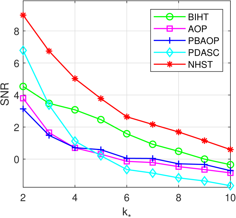
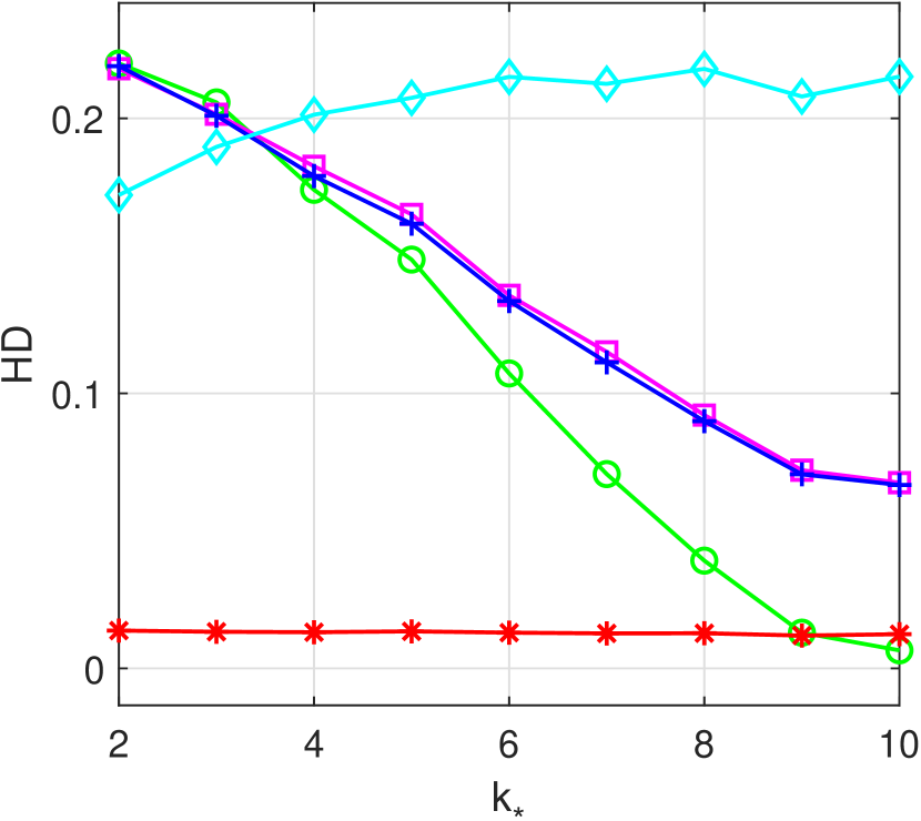
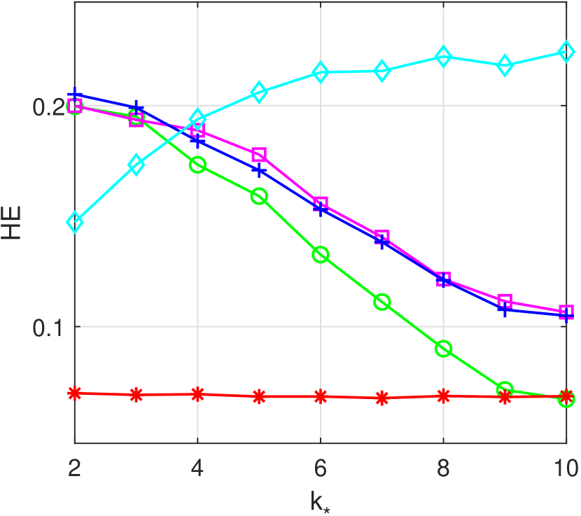
  Figure 2: Effect to $k_{*}$ Example 5.3.

• Effect to $m/n$ from $\{0.1,0.2,\cdots,0.7\}$ with fixing $n=256,k_{*}=\lceil 0.01n\rceil$ and $r=0.05$. As shown in Figure 4, again, NHST gets the smallest HD and HE for each $k_{*}$. In terms of SNR, NHST outperforms others when $m/n<0.4$ and PDASC behaves outstandingly for the bigger $m/n$. Similar observations can be seen for Example 5.2 and were omitted.

  

  

  

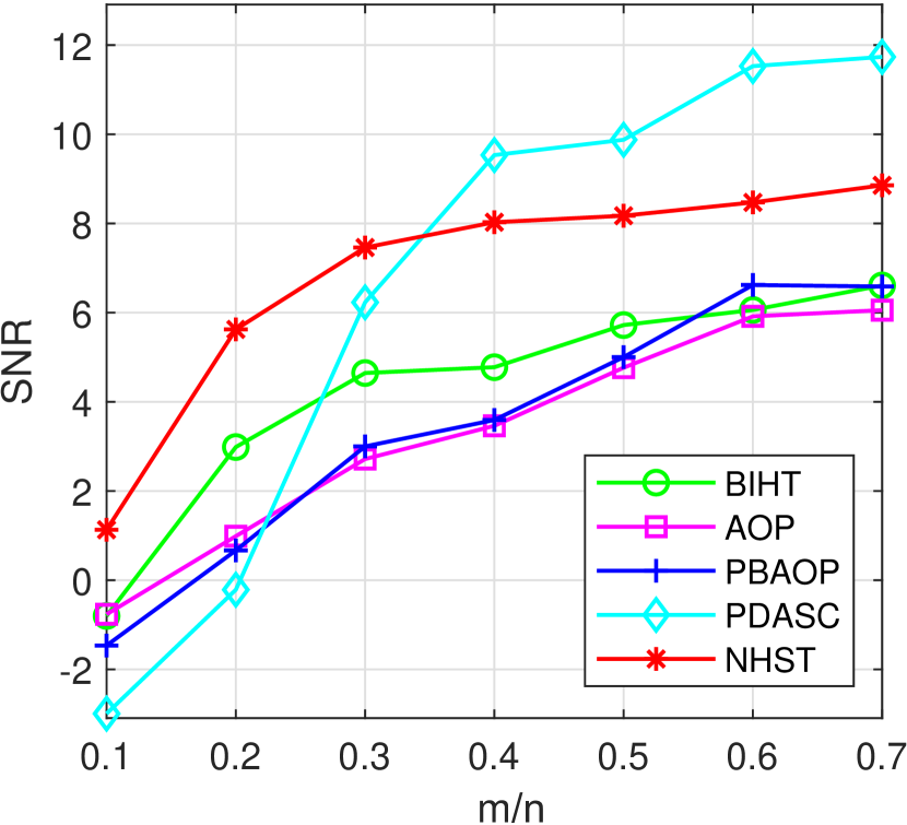
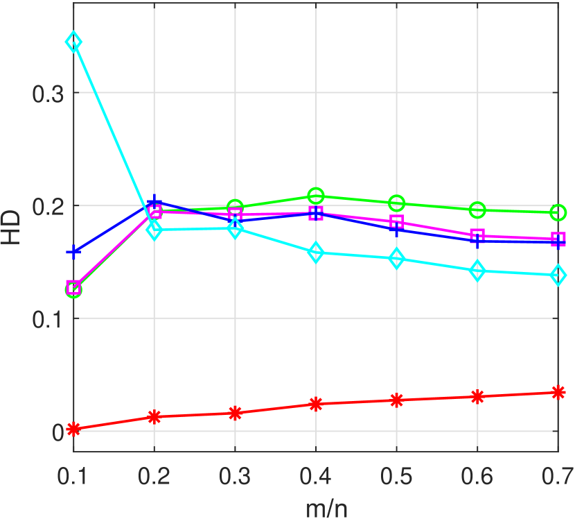
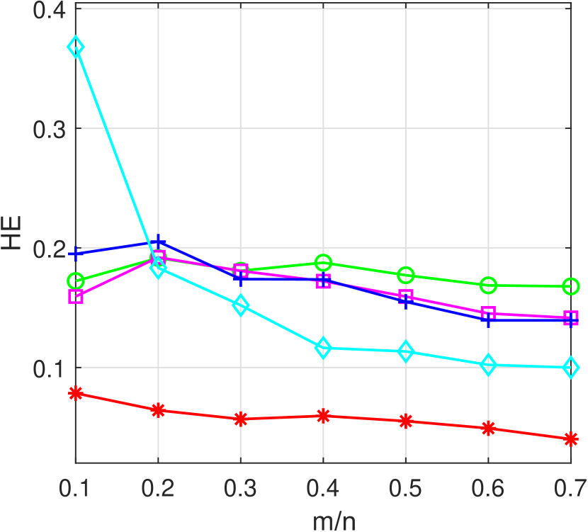
  Figure 3: Effect to $m/n$ for Example 5.3.

• Effect to $r$ from $\{0.02,0.02,\cdots,0.2\}$ with fixing $n=256,m=64$ and $k_{*}=\lceil 0.01n\rceil$. Average results for Example 5.3 are reported in Figure 4. As expected, NHST behaves the best in terms of delivering the highest SNR, the lowest HD and HE for each scenario. Again, we omitted the similar results for Example 5.2.

  

  

  

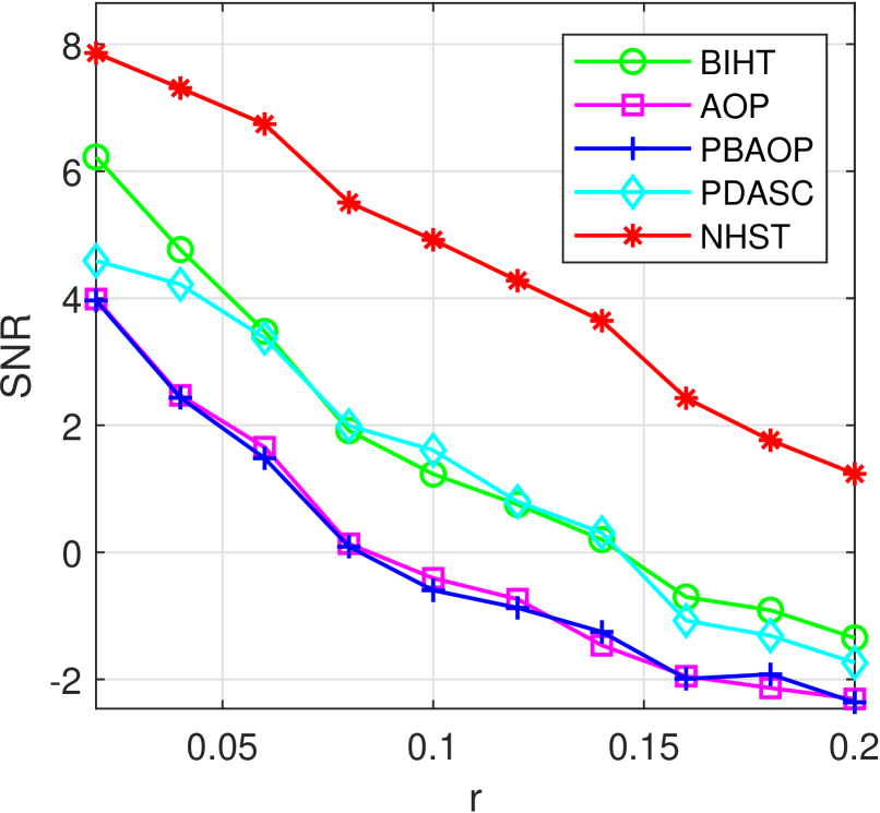
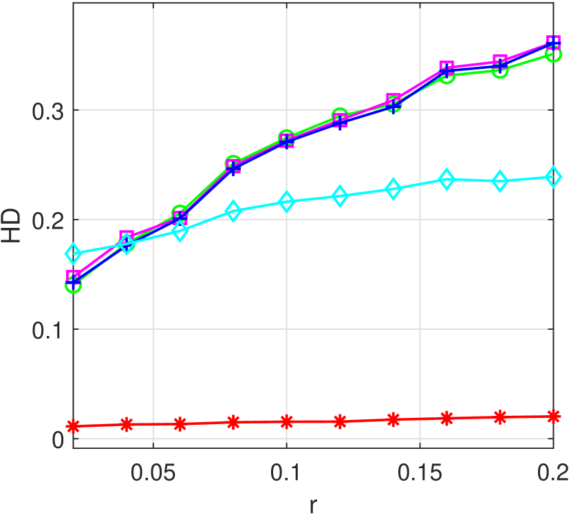
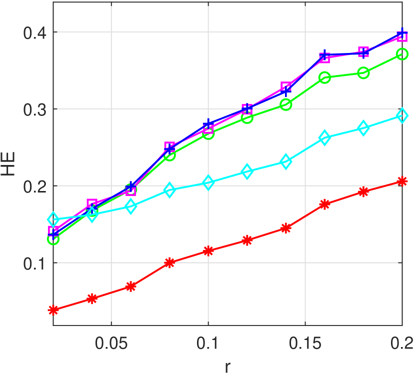
  Figure 4: Effect to $r$ for Example 5.3.

• Effect to $n$ from $\{1,2,3,4\}\times 5000$ with fixing $m=\lceil 0.25n\rceil,k_{*}=\lceil 0.01n\rceil$ and $r=0.05$. We record the average results in Table 3. Obviously, NHST achieves the highest SNR, lowest HD and HE but with consuming the shortest computational time. So it performs the best.

Table 3: Effect to the bigger values of $n$.

	Example 5.2						Example 5.3
$n$	BIHT	AOP	PBAOP	PDASC	NHST		BIHT	AOP	PBAOP	PDASC	NHST
	SNR						SNR
5000	4.485	1.883	2.360	0.787	5.753		4.985	1.762	2.193	1.417	5.420
10000	4.399	1.830	2.081	-0.133	5.478		4.826	1.574	1.939	0.004	5.470
15000	4.357	1.861	2.186	-1.060	5.455		4.889	1.692	2.024	-0.839	5.402
20000	4.425	1.770	2.242	-1.011	5.472		5.008	1.895	2.203	-1.456	5.143
	HD						HD
5000	0.167	0.161	0.162	0.321	0.034		0.168	0.155	0.160	0.293	0.036
10000	0.170	0.163	0.171	0.353	0.034		0.171	0.164	0.167	0.342	0.036
15000	0.170	0.166	0.170	0.392	0.034		0.163	0.152	0.158	0.379	0.036
20000	0.169	0.164	0.172	0.453	0.034		0.159	0.148	0.160	0.409	0.036
	HE						HE
5000	0.156	0.158	0.155	0.305	0.040		0.153	0.148	0.153	0.276	0.041
10000	0.158	0.158	0.163	0.339	0.041		0.158	0.157	0.160	0.327	0.041
15000	0.158	0.161	0.162	0.381	0.042		0.149	0.147	0.152	0.367	0.041
20000	0.157	0.160	0.163	0.445	0.041		0.145	0.141	0.149	0.401	0.042
	Time(in seconds)						Time(in seconds)
5000	0.676	1.220	0.576	0.181	0.107		0.688	1.247	0.528	0.182	0.122
10000	6.759	5.903	3.222	0.806	0.456		6.335	6.202	2.811	0.778	0.489
15000	15.37	14.64	7.296	1.843	1.080		14.85	13.03	6.982	1.868	1.159
20000	29.14	26.08	14.09	3.597	2.344		28.80	23.29	14.06	3.412	2.236

6 Conclusion

The Heaviside step function ideally characterizes the binary status of some real-world data. However, the hardness stemmed from the dis-continuity restricts its applications for a time. Fortunately, this paper manages to address the optimization (1.1) with the Heaviside set constraint. One of the key factors of such a success is based on the closed form of the normal cone to the feasible set, namely, the Heaviside step set (1.3). Another key factor is the establishment of the $\tau$-stationary point, which enables us to benefit from the Newton type method. We feel that those results could be extended to a more general case where $A{\bf x}-{\bf b}$ in the problem (1.1) is replaced by some nonlinear functions $c({\bf x})$. A possible explanation can be given as follows: For the optimization problem $\min\{f({\bf x}):c({\bf x})\leq 0\}$, if only a few (e.g., $s\ll m$) inequalities allow to be violated in the constraints, then $\|(c({\bf x}))_{+}\|_{0}\leq s$. Moreover, it is also worth applying the Heaviside set constrained optimization into dealing with some other relevant problems, such as the maximum rank correlation estimation for the linear transformation regression in statistics[15, 37, 24] and the area under the receiver operating characteristic curve in medicine [26, 33, 27, 46, 14].

7 Appendix

Similar to the definitions in (4.30), we denote

(7.1) $${\bf w}:=({\bf x};{\bf{\boldsymbol{\lambda}}}),~{}~{}{\bf y}:=A{\bf x}-{\bf b},~{}~{}~{}{\bf z}:={\bf y}+\tau{\bf{\boldsymbol{\lambda}}}.$$

To prove Theorem 4.2, we first prove the following lemma.

Lemma 7.1

Let ${\bf w}^{*}$ be a $\tau$-stationary point with $0<\tau<\tau_{*}$ of the problem (1.1) and $c_{*},C_{*},\tau_{*}$ be given by (4.3). The following results hold.

• There is a $\delta_{*}>0$ such that for any ${\bf w}\in U({\bf w}^{*},\delta_{*})$ and any $T\in{\mathbb{T}}_{\tau}({\bf z};s)$,

  (7.2) $$F({\bf w}^{*};T)=0.$$

• Suppose Assumptions 4.1 and 4.2 hold. There always exists a $\delta_{*}>0$ such that for any ${\bf w}\in U({\bf w}^{*},\min\{{\delta_{*}},{1}/({c_{*}L_{*}})\})$ and any $T\in{\mathbb{T}}_{\tau}({\bf z};s)$,

  (7.3) $$0<1/c_{*}\leq\sigma_{\min}(\nabla F({\bf w};T))~{}\leq\|\nabla F({\bf w};T)\|~{}\leq C_{*}.$$

Proof   a) Recall $J_{*}$ in (3.35) and ${\bf y}^{*}=A{\bf x}^{*}-{\bf b}$ by (4.30) that

$$J_{*}=\{i\in{\mathbb{N}}_{m}:(A{\bf x}^{*}-{\bf b})_{i}=0\}=\{i\in{\mathbb{N}}_{m}:~{}y^{*}_{i}=0\}.$$

This and ${\bf w}^{*}$ being a $\tau$-stationary point with $0<\tau<\tau_{*}$ satisfying (3.47) lead to

(7.4) $$\lambda_{i}^{*}=0,~{}y_{i}^{*}\neq 0,~{}i\in\overline{J}_{*},~{}~{}~{}~{}0\leq\lambda_{i}^{*}\leq y^{*}_{[s]}/\tau,~{}y_{i}^{*}=0,~{}i\in J_{*}.$$

Based on which, decompose ${\bf z}^{*}$ as

(7.9) $${\bf z}^{*}={\bf y}^{*}+\tau{\bf{\boldsymbol{\lambda}}}^{*}=\left[\begin{array}[]{ccc}{\bf y}^{*}_{J_{*}}+\tau{\bf{\boldsymbol{\lambda}}}^{*}_{J_{*}}\\ {\bf y}^{*}_{\overline{J}_{*}}+\tau{\bf{\boldsymbol{\lambda}}}^{*}_{\overline{J}_{*}}\end{array}\right]=\left[\begin{array}[]{r}\tau{\bf{\boldsymbol{\lambda}}}^{*}_{J_{*}}\\ {\bf y}^{*}_{\overline{J}_{*}}\end{array}\right].$$

Note that $y^{*}_{[s]}>0$ and $\max_{i}\lambda_{i}^{*}>0$ if ${\bf{\boldsymbol{\lambda}}}\neq 0$ by (7.4), so $\tau_{*}$ in (4.3) is well defined, which together with $0<\tau<\tau_{*}$ indicates

(7.10) $${y^{*}_{[s]}}-\tau\max_{i}\lambda_{i}^{*}>{y^{*}_{[s]}}-\tau_{*}\max_{i}\lambda_{i}^{*}\overset{\eqref{constants}}{=}0.$$

For any $T_{*}\in{\mathbb{T}}_{\tau}({\bf z}^{*};s)$, we have ${\mathbb{N}}_{m}=\Gamma_{+}^{*}\cup\Gamma_{-}^{*}\cup\Gamma_{0}^{*}$ by (1.12) and

(7.11) $$T_{*}=(\Gamma_{+}^{*}\setminus\Gamma_{s}^{*})\cup\Gamma_{0}^{*},~{}~{}\overline{T}_{*}=\Gamma_{s}^{*}\cup\Gamma_{-}^{*},~{}~{}\Gamma_{s}^{*}\subseteq\Gamma_{+}^{*}.$$

From (7.9) and (7.10), $\overline{J}_{*}$ contains all indices of $s$ largest elements and all indices of negative elements of ${\bf z}^{*}$ if $\|{\bf y}_{+}^{*}\|_{0}=s$, namely,

(7.12) $$\overline{J}_{*}=\overline{T}_{*},~{}~{}|\Gamma^{*}_{s}|=\|{\bf y}^{*}_{+}\|_{0},~{}~{}J_{*}=T_{*}.$$

It is easy to check that (7.12) also holds if $\|{\bf y}_{+}^{*}\|_{0}<s$ (Under such a case $\Gamma^{*}_{s}=\Gamma^{*}_{+}$ and $T_{*}=\Gamma_{0}^{*}$). Similarly, for any $T\in{\mathbb{T}}_{\tau}({\bf z};s)$, we have ${\mathbb{N}}_{m}=\Gamma_{+}\cup\Gamma_{-}\cup\Gamma_{0}$ and

(7.13) $$T=(\Gamma_{+}\setminus\Gamma_{s})\cup\Gamma_{0},~{}~{}\overline{T}=\Gamma_{s}\cup\Gamma_{-},~{}~{}\Gamma_{s}\subseteq\Gamma_{+}.$$

One can easily show that there is a sufficiently small $\delta_{*}>0$ (relied on ${\bf w}^{*}$) such that for ${\bf w}\in U({\bf w}^{*},\delta_{*})$ and any $T\in{\mathbb{T}}_{\tau}({\bf z};s)$,

(7.14) $$\Gamma_{-}^{*}\subseteq\Gamma_{-},~{}\Gamma_{+}^{*}\subseteq\Gamma_{+},~{}\Gamma_{s}^{*}\subseteq\Gamma_{s}$$

due to $z_{i}^{*}<0,\forall i\in\Gamma_{-}^{*}$ and $z_{i}^{*}>0,\forall i\in\Gamma_{+}^{*}$. We just show one of them. If $\Gamma_{-}^{*}\subseteq\Gamma_{-}$ is not true, then there is a $i\in\Gamma_{-}^{*}$ but $i\notin\Gamma_{-}$. This means $z_{i}\geq 0$ and $z_{i}^{*}<0$, which deliver $\|{\bf z}-{\bf z}^{*}\|\geq|z_{i}-z_{i}^{*}|\geq|z_{i}^{*}|$. On the other hand, by (4.30) and (7.1) one can derive $\|{\bf z}-{\bf z}^{*}\|\leq\max\{\|A\|,\tau\}\|{\bf w}-{\bf w}^{*}\|$, causing a contradiction due to $\delta_{*}$ being small enough. Therefore, those relations in (7.14) are true and imply

(7.15) $$\overline{T}_{*}=(\Gamma_{s}^{*}\cup\Gamma_{-}^{*})\subseteq(\Gamma_{s}\cup\Gamma_{-})=\overline{T},~{}~{}T\subseteq T_{*}.$$

Moreover, let $\Delta:=(\overline{T}\setminus\overline{T}_{*})=(T_{*}\setminus T)$. Recall that $T_{*}=(\Gamma_{+}^{*}\setminus\Gamma_{s}^{*})\cup\Gamma_{0}^{*}$ from (7.11) and $T=(\Gamma_{+}\setminus\Gamma_{s})\cup\Gamma_{0}$ from (7.13). If $|\Gamma_{s}^{*}|<s$, then by (2.1), we have $\Gamma_{s}^{*}=\Gamma_{+}^{*}$. So $T_{*}=\Gamma_{0}^{*}$ and $\Delta\subseteq\Gamma_{0}^{*}$. If $|\Gamma_{s}^{*}|=s$, then

$$s=|\Gamma_{s}^{*}|\overset{\eqref{JGG}}{\leq}|\Gamma_{s}|=\min\{s,|\Gamma_{+}|\}\overset{\eqref{T-z}}{\leq}s.$$

So $\Gamma_{s}^{*}=\Gamma_{s}$ and $(\Gamma_{+}^{*}\setminus\Gamma_{s}^{*})\subseteq(\Gamma_{+}\setminus\Gamma_{s})$ by (7.14), which also shows

(7.16) $$\Delta=(T_{*}\setminus T)\subseteq\Gamma_{0}^{*}.$$

We are ready to prove that for any ${\bf w}\in U({\bf w}^{*},\delta_{*})$ and any $T\in{\mathbb{T}}_{\tau}({\bf z};s)$,

(7.20) $$F({\bf w}^{*};T)=\left[\begin{array}[]{c}\nabla f({\bf x}^{*})+A^{\top}_{T}{\bf{\boldsymbol{\lambda}}}^{*}_{T}\\ A_{T}{\bf x}^{*}-{\bf b}_{T}\\ {\bf{\boldsymbol{\lambda}}}^{*}_{\overline{T}}\\ \end{array}\right]=0.$$

In fact, it follows from Theorem 4.1 and $J_{*}=T_{*}$ by (7.12) that the $\tau$-stationary point stationary point ${\bf w}^{*}$ of (1.1) satisfies the conditions

$$\nabla f({\bf x}^{*})+A^{\top}_{T_{*}}{\bf{\boldsymbol{\lambda}}}^{*}_{T_{*}} = 0,$$

(7.21) $$A_{T_{*}}{\bf x}^{*}-{\bf b}_{T_{*}} = 0,$$

$${\bf{\boldsymbol{\lambda}}}^{*}_{\overline{T}_{*}}=0,~{}~{}{\bf z}^{*}_{\Gamma_{0}^{*}} = 0,$$

for any $T_{*}\in{\mathbb{T}}_{\tau}({\bf z}^{*};s)$, where the last one is from the definition of $\Gamma_{0}^{*}$ in (1.12). These conditions enable us to obtain three facts:

• $A_{T}{\bf x}^{*}-{\bf b}_{T}=0$ due to $T\subseteq T_{*}$ by (7.15).

• As $\Delta\subseteq\Gamma_{0}^{*}\subseteq T_{*}$ by (7.16), we have ${\bf z}^{*}_{\Delta}=0,(A{\bf x}^{*}-{\bf b})_{\Delta}=0$ and thus $\tau{\bf{\boldsymbol{\lambda}}}^{*}_{\Delta}={\bf z}^{*}_{\Delta}-(A{\bf x}^{*}-{\bf b})_{\Delta}=0$. This suffices to ${\bf{\boldsymbol{\lambda}}}^{*}_{\overline{T}}={\bf{\boldsymbol{\lambda}}}^{*}_{\overline{T}_{*}\cup(\overline{T}\setminus\overline{T}_{*})}={\bf{\boldsymbol{\lambda}}}^{*}_{\overline{T}_{*}\cup\Delta}=0$.

• By ${\bf{\boldsymbol{\lambda}}}^{*}_{\overline{T}}=0$ and ${\bf{\boldsymbol{\lambda}}}^{*}_{\overline{T}_{*}}=0$,

  $$\nabla f({\bf x}^{*})+A_{T}^{\top}{\bf{\boldsymbol{\lambda}}}^{*}_{T}=\nabla f({\bf x}^{*})+A^{\top}{\bf{\boldsymbol{\lambda}}}^{*}=\nabla f({\bf x}^{*})+A_{T_{*}}^{\top}{\bf{\boldsymbol{\lambda}}}^{*}_{T_{*}}=0.$$

Overall, the above three facts verify (7.20), claiming the conclusion.

b) For any two matrices $D$ and $D^{\prime}$, we have

(7.22) $$\|D^{\prime}-D\| \geq \max_{i}|\sigma_{i}(D^{\prime})-\sigma_{i}(D)|$$

$$\geq |\sigma_{i_{0}}(D^{\prime})-\sigma_{i_{0}}(D)|$$

$$\geq \sigma_{i_{0}}(D^{\prime})-\sigma_{\min}(D)$$

$$\geq \sigma_{\min}(D^{\prime})-\sigma_{\min}(D),$$

where the first inequality holds from [25, Reminder (2), on Page 76] and $i_{0}$ satisfies $\sigma_{i_{0}}(D)=\sigma_{\min}(D)$. Recall $H(J)$ in (4.30) that

(7.27) $$H(J)\overset{\eqref{constants-y-H}}{=}\left[\begin{array}[]{ccc}\nabla^{2}f({\bf x}^{*})&A^{\top}_{J}\\ A_{J}&0\end{array}\right],~{}~{}~{}~{}\nabla F({\bf w}^{*};T)=\left[\begin{array}[]{cc}H(T)&0\\ 0&I\end{array}\right].~{}~{}~{}~{}~{}$$

It follows from the full row rankness of $A_{J_{*}}$ in Assumption 4.1 that $A_{J}$ is full row rank for any $J\subseteq J_{*}$. Again by Assumption 4.1, we have $H(J)$ is non-singular for any $J\subseteq J_{*}$, namely $\sigma_{\min}(H(J))>0$. As a result,

(7.28) $$1/c_{*}\overset{\eqref{constants}}{=}\min\{\min_{J\subseteq J_{*}}\sigma_{\min}(H(J)),1\}/2>0.$$

From a), there is a $\delta_{*}>0$ such that for any ${\bf w}\in U({\bf w}^{*},\delta_{*})$ and any $T\in{\mathbb{T}}_{\tau}({\bf z};s)$

(7.29) $$T\overset{\eqref{JGG1}}{\subseteq}T_{*}\overset{\eqref{G*y*}}{=}J_{*},$$

which means $H(T)$ is a submatrix of $H(J_{*})$. Then by [40, Theorem 1] that the maximum singular value of a matrix is no less than the maximum singular value of its sub-matrix, we obtain

(7.30) $$\|H(T)\|\leq\|H(J_{*})\|,~{}~{}\sigma_{\min}(H(T))\overset{\eqref{JJoG0-0}}{\geq}\min_{J\subseteq J_{*}}\sigma_{\min}(H(J)).$$

For any ${\bf w}\in U({\bf w}^{*},\min\{{\delta_{*}},{1}/({c_{*}L_{*}})\})$, the locally Lipschitz continuity of $\nabla^{2}f$ around ${\bf x}^{*}$ with $L_{*}>0$ leads to

(7.31) $$\|\nabla F({\bf w};T)-\nabla F({\bf w}^{*};T)\| \overset{\eqref{sta-eq-2}}{=} \|\nabla^{2}f({\bf x})-\nabla^{2}f({\bf x}^{*})\|$$

$$\overset{\eqref{Hessian-Lip}}{\leq} L_{*}\|{\bf x}-{\bf x}^{*}\|\leq L_{*}\|{\bf w}-{\bf w}^{*}\|<1/c_{*},~{}~{}$$

which contributes to

$$\|\nabla F({\bf w};T)\| \leq \|\nabla F({\bf w}^{*};T)\|+\|\nabla F({\bf w};T)-\nabla F({\bf w}^{*};T)\|$$

$$\overset{\eqref{HH*2}}{\leq} \|\nabla F({\bf w}^{*};T)\|+1/c_{*}$$

$$\overset{\eqref{FH*-FG}}{=} \max\{\|H(T)\|,1\}+1/c_{*}$$

$$\overset{\eqref{JJoG0-H}}{\leq} \max\{\|H(J_{*})\|,1\}+1/c_{*}$$

$$\leq 2\max\{\|H(J_{*})\|,1\}\overset{\eqref{constants}}{=}C_{*}.$$

Next we show the smallest singular value of $\nabla F({\bf w};T)$ has a lower bound. In fact,

$$\sigma_{\min}(\nabla F({\bf w};T)) \overset{\eqref{D-D}}{\geq} \sigma_{\min}(\nabla F({\bf w}^{*};T))-\|\nabla F({\bf w}^{*};T)-\nabla F({\bf w};T)\|$$

$$\overset{\eqref{HH*2}}{\geq} \sigma_{\min}(\nabla F({\bf w}^{*};T))-1/c_{*}$$

$$\overset{\eqref{FH*-FG}}{=} \min\{\sigma_{\min}(H(T)),1\}-1/c_{*}$$

$$\overset{\eqref{JJoG0-H}}{\geq} \min\{\min_{J\subseteq J_{*}}\sigma_{\min}(H(J)),1\}-1/c_{*}$$

$$\overset{\eqref{1-c-*}}{=} 2/c_{*}-1/c_{*}=1/c_{*}.$$

Hence, the whole proof is completed. . $\Box$

The proof of Theorem 4.2

Proof   a) Let $\epsilon_{*}:=\min\{{\delta_{*}},{1}/({c_{*}L_{*}})\}$. Then

(7.32) $$\epsilon_{*}c_{*}L_{*}\leq 1.$$

It follows from Lemma 7.1 and ${\bf w}^{0}\in U({\bf w}^{*},\epsilon_{*})$ that

(7.33) $$F({\bf w}^{*};T_{0})\overset{\eqref{gw*-0}}{=}0,~{}~{}~{}\|(\nabla F({\bf w}^{0};T_{0}))^{-1}\|\overset{\eqref{bd-h-0}}{\leq}c_{*}$$

for the $T_{0}\in{\mathbb{T}}_{\tau}({\bf z}^{0};s)$. From (4.13), we have

(7.34) $$\nabla F({\bf w}^{0};T_{0})~{}{\bf d}^{0}=-F({\bf w}^{0};T_{0}).$$

Lemma 7.1 c) states that $\nabla F({\bf w}^{0};T_{0})$ is non-singular and thus ${\bf d}^{0}$ is well defined. Let ${\bf w}^{0}_{\beta}={\bf w}^{*}+\beta({\bf w}^{0}-{\bf w}^{*})$ where $\beta\in[0,1]$. One can easily check that ${\bf w}^{0}_{\beta}\in U({\bf w}^{*},\epsilon_{*})$ as $\|{\bf w}^{0}_{\beta}-{\bf w}^{*}\|=\beta\|{\bf w}^{0}-{\bf w}^{*}\|\leq\epsilon_{*}.$ For notational simplicity, let $\nabla F^{0}:=\nabla F({\bf w}^{0};T_{0})$ and $\nabla F^{0}_{\beta}:=\nabla F({\bf w}^{0}_{\beta};T_{0})$.The locally Lipschitz continuity of $\nabla^{2}f(\cdot)$ around ${\bf x}^{*}$ with $L_{*}>0$ brings out

(7.35) $$\|\nabla F^{0}-\nabla F^{0}_{\beta}\| \overset{\eqref{sta-eq-2}}{=} \|\nabla^{2}f({\bf x}^{0})-\nabla^{2}f({\bf x}^{0}_{\beta})\|$$

$$\overset{\eqref{Hessian-Lip}}{\leq} L_{*}\|{\bf x}^{0}-{\bf x}^{0}_{\beta}\|\leq L_{*}\|{\bf w}^{0}-{\bf w}^{0}_{\beta}\|$$

$$= L_{*}(1-\beta)\|{\bf w}^{0}-{\bf w}^{*}\|.$$

Note that for the fixed $T_{0}$, the function $F(\cdot;T_{0})$ is differentiable. So we have the following mean value expression

(7.36) $$F({\bf w}^{0};T_{0}) = F({\bf w}^{*};T_{0})+\int_{0}^{1}\nabla F^{0}_{\beta}\cdot({\bf w}^{0}-{\bf w}^{*})d\beta$$

$$\overset{\eqref{gw*-bd-h}}{=} \int_{0}^{1}\nabla F^{0}_{\beta}\cdot({\bf w}^{0}-{\bf w}^{*})d\beta.$$

Then the following chain of inequalities hold.

(7.37) $$\|{\bf w}^{1}-{\bf w}^{*}\| = \|{\bf w}^{0}+{\bf d}^{0}-{\bf w}^{*}\|$$

$$\overset{\eqref{dkt}}{=} \|{\bf w}^{0}-{\bf w}^{*}-(\nabla F^{0})^{-1}\cdot F({\bf w}^{0};T_{0})\|$$

$$\overset{\eqref{gw*-bd-h}}{\leq} c_{*}\|\nabla F^{0}\cdot({\bf w}^{0}-{\bf w}^{*})-F({\bf w}^{0};T_{0})\|$$

$$\overset{\eqref{mean-value}}{=} c_{*}\|\nabla F^{0}\cdot({\bf w}^{0}-{\bf w}^{*})-\int_{0}^{1}\nabla F^{0}_{\beta}\cdot({\bf w}^{0}-{\bf w}^{*})d\beta\|$$

$$\leq c_{*}\int_{0}^{1}\|\nabla F^{0}-\nabla F^{0}_{\beta}\|\|{\bf w}^{0}-{\bf w}^{*}\|d\beta$$

$$\overset{\eqref{lipschitz}}{\leq} c_{*}L_{*}\int_{0}^{1}(1-\beta)\|{\bf w}^{0}-{\bf w}^{*}\|\|{\bf w}^{0}-{\bf w}^{*}\|d\beta$$

$$= 0.5c_{*}L_{*}\|{\bf w}^{0}-{\bf w}^{*}\|^{2}.$$

The above relation suffices to

(7.38) $$\|{\bf w}^{1}-{\bf w}^{*}\|\leq 0.5c_{*}L_{*}\epsilon_{*}\|{\bf w}^{0}-{\bf w}^{*}\|\overset{\eqref{radius}}{\leq}0.5\|{\bf w}^{0}-{\bf w}^{*}\|<\epsilon_{*}.$$

This means ${\bf w}^{1}\in U({\bf w}^{*},\epsilon_{*})$. Replacing $T_{0}$ by $T_{1}$, the same reasoning allows us to show that ${\bf d}^{1}$ is well defined and $\|{\bf w}^{2}-{\bf w}^{*}\|\leq 0.5c_{*}L_{*}\|{\bf w}^{1}-{\bf w}^{*}\|^{2}$. By the induction, we can conclude that ${\bf w}^{k}\in U({\bf w}^{*},\epsilon_{*})$, ${\bf d}^{k}$ is well defined and

(7.39) $$\|{\bf w}^{k+1}-{\bf w}^{*}\| \leq 0.5c_{*}L_{*}\|{\bf w}^{k}-{\bf w}^{*}\|^{2},$$

(7.40) $$\leq 0.5c_{*}L_{*}\epsilon_{*}\|{\bf w}^{k}-{\bf w}^{*}\|\overset{\eqref{radius}}{\leq}0.5\|{\bf w}^{k}-{\bf w}^{*}\|.$$

Therefore, (7.39) claims b). The conclusion of a) can be made by (7.40) that ${\bf w}^{k}\rightarrow{\bf w}^{*}$ and ${\bf d}^{k}={\bf w}^{k+1}-{\bf w}^{k}={\bf w}^{k+1}-{\bf w}^{*}+{\bf w}^{*}-{\bf w}^{k}\rightarrow 0.$ . $\Box$

References

- [1] L. Ban, B. S. Mordukhovich, and W. Song. Lipschitzian stability of parametric variational inequalities over generalized polyhedra in banach spaces. Nonlinear Analysis: Theory, Methods & Applications, 74(2):441–461, 2011.
- [2] P. T. Boufounos and R. G. Baraniuk. 1-bit compressive sensing. In 2008 42nd Annual Conference on Information Sciences and Systems, pages 16–21. IEEE, 2008.
- [3] J. P. Brooks. Support vector machines with the ramp loss and the hard margin loss. Operations Research, 59(2):467–479, 2011.
- [4] E. J. Candes, M. B. Wakin, and S. P. Boyd. Enhancing sparsity by reweighted minimization. Journal of Fourier Analysis and Applications, 14(5-6):877–905, 2008.
- [5] C.-C. Chang and C.-J. Lin. LIBSVM: A library for support vector machines. ACM Transactions on Tntelligent Systems and Technology (TIST), 2(3):1–27, 2011.
- [6] R. Collobert, F. Sinz, J. Weston, and L. Bottou. Large scale transductive svms. Journal of Machine Learning Research, 7(Aug):1687–1712, 2006.
- [7] C. Cortes and V. Vapnik. Support-vector networks. Machine Learning, 20(3):273–297, 1995.
- [8] D.-Q. Dai, L. Shen, Y. Xu, and N. Zhang. Noisy 1-bit compressive sensing: models and algorithms. Applied and Computational Harmonic Analysis, 40(1):1–32, 2016.
- [9] T. Evgeniou, M. Pontil, and T. Poggio. Regularization networks and support vector machines. Advances in Computational Mathematics, 13(1):1, 2000.
- [10] R.-E. Fan, K.-W. Chang, C.-J. Hsieh, X.-R. Wang, and C.-J. Lin. Liblinear: A library for large linear classification. Journal of Machine Learning Research, 9(Aug):1871–1874, 2008.
- [11] Y. Feng, Y. Yang, X. Huang, S. Mehrkanoon, and J. A. Suykens. Robust support vector machines for classification with nonconvex and smooth losses. Neural Computation, 28(6):1217–1247, 2016.
- [12] J. H. Friedman. On bias, variance, 0/1 loss, and the curse-of-dimensionality. Data Mining and Knowledge Discovery, 1(1):55–77, 1997.
- [13] D. Gale. The theory of linear economic models. University of Chicago Press, 1989.
- [14] H. Ghanbari, M. Li, and K. Scheinberg. Novel and efficient approximations for zero-one loss of linear classifiers. arXiv preprint arXiv:1903.00359, 2019.
- [15] A. K. Han. Non-parametric analysis of a generalized regression model: the maximum rank correlation estimator. Journal of Econometrics, 35(2-3):303–316, 1987.
- [16] T. Hastie, R. Tibshirani, and J. Friedman. The elements of statistical learning: data mining, inference, and prediction. Springer Science & Business Media, 2009.
- [17] J. Huang, Y. Jiao, X. Lu, and L. Zhu. Robust decoding from 1-bit compressive sampling with ordinary and regularized least squares. SIAM Journal on Scientific Computing, 40(4):A2062–A2086, 2018.
- [18] X. Huang, L. Shi, and J. A. Suykens. Support vector machine classifier with pinball loss. IEEE Transactions on Pattern Analysis and Machine Intelligence, 36(5):984–997, 2013.
- [19] X. Huang, L. Shi, M. Yan, and J. A. Suykens. Pinball loss minimization for one-bit compressive sensing: Convex models and algorithms. Neurocomputing, 314:275–283, 2018.
- [20] L. Jacques, J. N. Laska, P. T. Boufounos, and R. G. Baraniuk. Robust 1-bit compressive sensing via binary stable embeddings of sparse vectors. IEEE Transactions on Information Theory, 59(4):2082–2102, 2013.
- [21] M.-J. Lai, Y. Xu, and W. Yin. Improved iteratively reweighted least squares for unconstrained smoothed minimization. SIAM Journal on Numerical Analysis, 51(2):927–957, 2013.
- [22] J. N. Laska, Z. Wen, W. Yin, and R. G. Baraniuk. Trust, but verify: Fast and accurate signal recovery from 1-bit compressive measurements. IEEE Transactions on Signal Processing, 59(11):5289–5301, 2011.
- [23] L. Li and H.-T. Lin. Optimizing 0/1 loss for perceptrons by random coordinate descent. In 2007 International Joint Conference on Neural Networks, pages 749–754. IEEE, 2007.
- [24] H. Lin and H. Peng. Smoothed rank correlation of the linear transformation regression model. Computational Statistics & Data Analysis, 57(1):615–630, 2013.
- [25] H. Lütkepohl. Handbook of matrices, volume 1. Wiley Chichester, 1996.
- [26] S. Ma and J. Huang. Regularized ROC method for disease classification and biomarker selection with microarray data. Bioinformatics, 21(24):4356–4362, 2005.
- [27] S. Ma and J. Huang. Combining multiple markers for classification using ROC. Biometrics, 63(3):751–757, 2007.
- [28] L. Mason, P. L. Bartlett, and J. Baxter. Improved generalization through explicit optimization of margins. Machine Learning, 38(3):243–255, 2000.
- [29] B. S. Mordukhovich and N. M. Nam. An easy path to convex analysis and applications. Synthesis Lectures on Mathematics and Statistics, 6(2):1–218, 2013.
- [30] T. Nguyen and S. Sanner. Algorithms for direct 0-1 loss optimization in binary classification. In International Conference on Machine Learning, pages 1085–1093, 2013.
- [31] E. Osuna and F. Girosi. Reducing the run-time complexity of support vector machines. In International Conference on Pattern Recognition (submitted), 1998.
- [32] K. Pelckmans, J. Suykens, T. Gestel, J. Brabanter, L. Lukas, B. Hamers, B. Moor, and J. Vandewalle. A matlab/c toolbox for least square support vector machines. ESATSCD-SISTA Technical Report, pages 02–145, 2002.
- [33] M. S. Pepe, T. Cai, and G. Longton. Combining predictors for classification using the area under the receiver operating characteristic curve. Biometrics, 62(1):221–229, 2006.
- [34] C.-T. Perng. On a class of theorems equivalent to Farkas’s lemma. Applied Mathematical Sciences, 11(44):2175–2184, 2017.
- [35] Y. Plan and R. Vershynin. Robust 1-bit compressed sensing and sparse logistic regression: A convex programming approach. IEEE Transactions on Information Theory, 59(1):482–494, 2012.
- [36] R. T. Rockafellar and R. J.-B. Wets. Variational analysis, volume 317. Springer Science & Business Media, 2009.
- [37] R. P. Sherman. The limiting distribution of the maximum rank correlation estimator. Econometrica: Journal of the Econometric Society, pages 123–137, 1993.
- [38] P. Sollich. Bayesian methods for support vector machines: Evidence and predictive class probabilities. Machine Learning, 46(1-3):21–52, 2002.
- [39] J. A. Suykens and J. Vandewalle. Least squares support vector machine classifiers. Neural Processing Letters, 9(3):293–300, 1999.
- [40] R. C. Thompson. Principal submatrices ix: Interlacing inequalities for singular values of submatrices. Linear Algebra and its Applications, 5(1):1–12, 1972.
- [41] B. Ustun and C. Rudin. Supersparse linear integer models for optimized medical scoring systems. Machine Learning, 102(3):349–391, 2016.
- [42] H. Wang, Y. Shao, S. Zhou, C. Zhang, and N. Xiu. Support vector machine classifier via soft-margin loss. arXiv preprint arXiv:1912.07418, 2019.
- [43] E. W. Weisstein. Heaviside step function. https://mathworld.wolfram.com/, 2002.
- [44] Y. Wu and Y. Liu. Robust truncated hinge loss support vector machines. Journal of the American Statistical Association, 102(479):974–983, 2007.
- [45] M. Yan, Y. Yang, and S. Osher. Robust 1-bit compressive sensing using adaptive outlier pursuit. IEEE Transactions on Signal Processing, 60(7):3868–3875, 2012.
- [46] X. Zhao, W. Dai, Y. Li, and L. Tian. Auc-based biomarker ensemble with an application on gene scores predicting low bone mineral density. Bioinformatics, 27(21):3050–3055, 2011.
- [47] H. Zou and T. Hastie. Regularization and variable selection via the elastic net. Journal of the Royal Statistical Society: Series B (Statistical Methodology), 67(2):301–320, 2005.