$\mathcal{PT}$-symmetry in compact phase space for a linear Hamiltonian

Abstract

We study the time evolution of a $\mathcal{PT}$-symmetric, non-Hermitian quantum system for which the associated phase space is compact. We focus on the simplest non-trivial example of such a Hamiltonian, which is linear in the angular momentum operators. In order to describe the evolution of the system, we use a particular disentangling decomposition of the evolution operator, which remains numerically accurate even in the vicinity of the Exceptional Point. We then analyze how the non-Hermitian part of the Hamiltonian affects the time evolution of two archetypical quantum states, coherent and Dicke states. For that purpose we calculate the Husimi distribution or $Q$ function and study its evolution in phase space. For coherent states, the characteristics of the evolution equation of the Husimi function agree with the trajectories of the corresponding angular momentum expectation values. This allows to consider these curves as the trajectories of a classical system. For other types of quantum states, e.g. Dicke states, the equivalence of characteristics and trajectories of expectation values is lost.

1 Introduction and motivation

Non-Hermitian quantum systems may still have a real spectrum, if they are $\mathcal{PT}$-symmetric Benderbook2018 . Since their introduction by Bender and Boettcher in 1998 BenderPRL1998 , these systems have found a wide range of applications HeissJPA2012 ; BenderJP2015 ; FengNature2017 ; El-GanainyNature2018 ; Miri2019 . One of the defining features of such systems is that the corresponding Hamiltonian may have real or complex eigenvalues. In the first case, one says that the $\mathcal{PT}$-symmetric phase is intact, in the second that it is broken. The transition between these phases occurs at so-called “Exceptional Points” (EPs), at which two or more eigenvalues and eigenvectors coalesce. In this case, the Hamiltonian becomes defective Katobook1995 . EPs have been related to many remarkable phenomena. Some recent examples are chirality PhysRevLett.86.787 ; Mailybaev2005 ; Peng2016 , unidirectional invisibility Regensburger2012 ; Lin2011 ; Feng2012 , enhanced sensing Chen2017 and the possibility to stop light GoldzakPRL2018 . From the transport point of view, a $\mathcal{PT}$-symmetric Hamiltonian offers a convenient way to describe a physical system with gains and losses. Such phenomena can be studied conveniently in tight-binding Hamiltonians JinPRA2009 ; YogeshPRA2010 ; OrtegaJPA2020 .

Only recently, $\mathcal{PT}$-symmetric systems have been studied from a semiclassical perspective, also GraefeJPA2010 ; GraefePRA2011 ; PraxmeyerPRA2016 . In this context it is natural to use phase space representations of the quantum system in question. These investigations have been focused mainly on systems described by the Heisenberg-Weyl algebra where the associated phase space is a two-dimensional plane. The case of a compact phase space, which corresponds to the angular momentum algebra has received much less attention, though note GraefeJPA2010 ; GrKoNi10 ; MudGra20 .

In this work, we provide a thorough analysis of the simplest non-trivial $\mathcal{PT}$-symmetric system, where the Hamiltonian is a linear function of the angular momentum operators. For such systems, the Bloch sphere plays the role of a classical phase space. In the case of a linear Hermitian Hamiltonian, the phase space representations (for instance Glauber, Wigner or Husimi) refI1 ; refI2 ; refI3 ; refI4 of the quantum system evolve along characteristics, conserving their function values – just as in the case of the classical Liouville equation. As a consequence, the expectation values of the angular momentum operators follow these characteristics also, and this allows one to identify them as classical trajectories.

In the case of a non-Hermitian and $\mathcal{PT}$-symmetric Hamiltonian, the situation is different: The evolution equations for the different quantum representations in phase space do no longer agree, and some of them may no longer be solved in terms of characteristics.

In this work we use the Husimi function, which can still be solved with the method of characteristics. There the only difference is that the function changes its value along the characteristics, which is equivalent to the existence of sources and sinks in the phase space. The expectation values of the angular momentum operators follow different trajectories, lying inside the Bloch ball, which depend on the complete shape of the quantum states. Surprisingly, it is still possible to return to the old unified picture. To achieve this, one has to limit to the evolution of coherent states. These states conserve their shape and follow the characteristcs of the evolution equation for the Husimi function. However, they do not conserve their norm. This allows one to speak of a corresponding classical system, where the trajectories represent localized excitations which may vary in intensity MudGra20 , according to the sources and sinks present in the system.

The paper is organized as follows. In Sec. 2, we describe our model and introduce the quantities of interest: the evolution operator, expectation values and the Husimi function (or $Q$ function). In Sec. 3 we present two methods to compute the evolution of the system, the diagonalization of the Hamiltonian with a non-unitary similarity transformation and the disentangling decomposition inspired by the decomposition of a general rotation using Euler angles. In Sec. 4 we discuss our results for the time evolution of the quantum system in phase space. After this we consider the Husimi function and the evolution of expectation values in Sec. 5. In the appendix, we collect a few general properties of expectation values and variances for coherent states and Dicke states (in App. A), derive the evolution equation for the Husimi function (in App. B) and the analytical solution to the Ehrenfest equation for the angular momentum expectation values (in App. C).

2 General definitions and the model

We are interested in systems where the dynamical symmetry group is $\operatorname{SO}(3)$. The angular momentum operators $\{{S_{x},S_{y},S_{z}\}}$ are the generators of the corresponding Lie algebra $\mathfrak{so}(3)$, and hence fulfill the commutation relations $[S_{x},S_{y}]=iS_{z}$ (and cyclic permutations of it). For simplicity, we set $\hbar=1$. The eigenvectors of the operator $S_{z}$ are the Dicke states $\left|S,m\right\rangle$, where

$$S_{z}\left|S,m\right\rangle=m\left|S,m\right\rangle\quad,\qquad-S\leq m\leq S$$ (1)

with $S$ being a positive integer. As the generator of the dynamics, we choose the simplest non-trivial, linear, PT-symmetric Hamiltonian,

$$H=2v\;S_{x}-2i\,\gamma\;S_{z}=H_{0}+i\;\Gamma\;,$$ (2)

with real parameters $\gamma$ and $v$, such that both operators $H_{0}$ and $\Gamma=-2\gamma S_{z}$ are Hermitian. This Hamiltonian can describe, under a Schwinger transformation, the motion of a non-interacting Bose-Einstein condensate in a two-well potential under $\mathcal{PT}$-symmetry GraefePRL2008 .

The Hamiltonian in Eq. (2) is $\mathcal{PT}$-symmetric. This means that there exist an antilinear (conjugated linear) operator $\mathcal{T}$ and a linear involution $\mathcal{P}$ (i.e. $\mathcal{P}=\mathcal{P}^{-1}$) which commute, $[\mathcal{T},\mathcal{P}]=0$, such that $[\mathcal{PT},H]=0$ MudGra20 ; JonMat10 . As a consequence the Hamiltonian may have real eigenvalues.

In our case, the parity operator may be defined by its action on the Dicke states:

$$\forall\;-S\leq m\leq S\quad:\quad\mathcal{P}\;|S,m\rangle=|S,-m\rangle\;,$$ (3)

and the time-reversal operator by its action on an arbitrary state written as a linear combination of the Dicke states:

$$\mathcal{T}\;\sum_{m}c_{m}\;|S,m\rangle=\sum_{m}c_{m}^{*}\;|S,m\rangle\;.$$ (4)

The operators $\mathcal{P}$ and $\mathcal{T}$ fulfill all the requirements mentioned above. In addition it holds that $\mathcal{T}^{2}=+\,\mathbb{1}$ such that we may speak of an “even” $\mathcal{PT}$ symmetry.

2.1 Evolution and expectation values

We find the solution of the Schrödinger equation

$$i\,\frac{d}{dt}\;|\Psi\rangle=H\;|\Psi\rangle\,$$ (5)

in terms of the non-unitary evolution operator

$$U(t)=e^{-iHt}\;.$$ (6)

Accordingly, we obtain for the evolution of the corrresponding density matrix

$$\varrho(t)=U(t)\;\varrho(0)\;U(t)^{\dagger}\;.$$ (7)

This shows that the density matrix $\varrho(t)$ does not remain normalized in general. However, $\rho\left(t\right)$ is Hermitian by construction, so its trace, and also the expectation values of observables calculated from it, are real.

Non-Hermitian Hamiltonians are typically used to describe quantum systems or wave-mechanical systems with gains and losses. In the single particle case, this implies that ${\rm tr}[\varrho(t)\,]\leq 1$ is the probability that the measurement of some observable $\hat{A}$ actually finds the particle and gives a valid result. In the case of many particles (e.g. a Bose-Einstein condensate) or a classical wave field, the density matrix describes the intensity of the field as it varies over time. In both cases, we calculate the expectation value of $\hat{A}$ using the density matrix as

$$\langle\hat{A}\rangle=\frac{{\rm tr}[\varrho(t)\,\hat{A}\,]}{{\rm tr}[\varrho(t)\,]}\;.$$ (8)

This is because in the single particle case, measuring $\hat{A}$ implies to average over many realizations of the measurement. Then, the only meaningful average is that over those realizations where the measurement was actually successful.

2.2 Husimi function

A useful method to visualize a quantum system consists in mapping its state $\varrho$ into a complex valued function defined on the corresponding classical phase space. According to Weyl Weyl and later Stratonovich and Moyal Stratonovich ; moyal there are several choices for such a mapping, which can be tagged by the parameter $s\in\{+1,0,-1\}$. In that case, the different values correspond to the $P$ (Glauber), $W$ (Wigner) and $Q$ (Husimi) functions, respectively. Since the dynamical symmetry group is $\operatorname{SO}(3)$, the classical phase space is the so-called Bloch sphere $\mathbb{S}^{2}$. For our purposes, we will use the (real positive) Husimi function, which is defined as

$$Q_{\varrho}(\theta,\phi)=\langle\theta,\phi|\varrho|\theta,\phi\rangle={\rm tr}\big{[}\,\varrho\,\hat{\omega}_{Q}(\theta,\phi)\,\big{]}\;,$$ (9)

where the angles $(\theta,\phi)$ parametrize the points in $\mathbb{S}^{2}$ and

$$|\theta,\phi\rangle=e^{-i\phi S_{z}}e^{-i\theta S_{y}}\left|S,S\right\rangle$$ (10)

is the coherent state refcoh with angular momentum expectation values

$$\begin{pmatrix}\langle S_{x}\rangle\\ \langle S_{y}\rangle\\ \langle S_{z}\rangle\end{pmatrix}=S\begin{pmatrix}\sin\theta\,\cos\phi\\ \sin\theta\,\sin\phi\\ \cos\theta\end{pmatrix}\;.$$ (11)

The kernel operator $\hat{\omega}_{Q}(\theta,\phi)=|\theta,\phi\rangle\langle\theta,\phi|$ can be written as

$$\hat{\omega}_{Q}(\theta,\phi)=\frac{2\sqrt{\pi}}{\sqrt{2S+1}}\sum_{L=0}^{2S}\sum_{M=-L}^{L}Y^{*}_{L,M}(\theta,\phi)\hat{T}^{(S)}_{L,M}C^{SS}_{SS;L0}\;,$$ (12)

where $Y_{L,M}(\Omega)=(-1)^{M}Y^{*}_{L,-M}(\Omega)$ is the standard spherical harmonic function. In Eq. (12) we used the irreducible tensor operators

$$\hat{T}^{(S)}_{L,M}=\sqrt{\frac{2L+1}{2S+1}}\sum_{m,m^{{}^{\prime}}=-S}^{S}C^{S,m^{{}^{\prime}}}_{S,m;L,M}|S,m^{{}^{\prime}}\rangle\langle S,m|.$$ (13)

Here $C^{S,m^{{}^{\prime}}}_{S,m;L,M}$ and $C^{SS}_{SS;L0}$ are the Clebsch-Gordan coefficients Varshalovichbook . The Husimi function is real and positive.

In order to study the dynamics generated by $H$, we choose as initial conditions two archetipycal states: a coherent state (semiclassical) and a Dicke state (no semiclassical). The Husimi function of a coherent state $|\theta_{0},\phi_{0}\rangle$ is

$$Q_{|\theta_{0},\phi_{0}\rangle}=\Big{(}\frac{1+\mathbf{n_{0}}\cdot\mathbf{n}}{2}\Big{)}^{2S},$$ (14)

which is a localized distribution in phase space, centered at the point $\mathbf{n_{0}}=(\sin\theta_{0}\cos\phi_{0},\sin\theta_{0}\sin\phi_{0},\cos\theta_{0})$ with the variables $(\theta,\phi)$ contained in $\mathbf{n}=(\sin\theta\cos\phi,\sin\theta\sin\phi,\cos\theta)$. Fig. 1(a) shows an example for $\theta_{0}=\pi/2,\phi_{0}=\pi/4$.

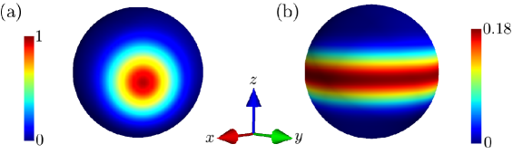
Figure 1: (a) Husimi function $Q_{|\theta_{0},\phi_{0}\rangle}$ of the coherent state with $\theta_{0}=\pi/2,\phi_{0}=\nicefrac{{\pi}}{{4}}$. (b) Husimi function of the Dicke state $|S=10,m=0\rangle$.

On the other hand, the Husimi function of a Dicke state is usually not localized,

$$Q_{|S,m\rangle}=\frac{1}{\sqrt{4\pi}}\sum_{L=0}^{2S}\sqrt{2L+1}\;Y^{*}_{L0}(\theta,\phi)\;C^{SS}_{SS;L0}C^{Sm}_{Sm;L0}\;.$$ (15)

For instance, the Husimi function of the state $\left|S,0\right\rangle$, is delocalized in the $\phi$-coordinate, as can be seen in Fig 1(b). General expressions for expectation values and variances of coherent states and Dicke states are collected in App. A.

3 Decomposition of the evolution operator

In this section, we consider two methods to calculate the evolution operator $U(t)$ from Eq. (6) analytically. The first is based on a similarity transformation which diagonalizes $H$. The second, so-called “disentangling method”, factorizes the evolution into three elementary parts.

3.1 Diagonalization method

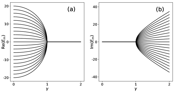
Figure 2: The eigenvalues $E_{m}$ of the Hamiltonian $H$, as given in Eq. (17) as a function of $\gamma$ for $S=10$ and $v=1$. In panel (a) the eigenvalues are real for $\gamma<v$, in panel (b) the eigenvalues are imaginary for $\gamma>v$. As $\gamma\to v$, all eigenvalues coalesce in a single EP.

Following GraefeJPA2008 , the Hamiltonian can be rewritten as

$$H=e^{\alpha S_{y}}\;\tilde{H}\;e^{-\alpha S_{y}}\;,\qquad\tilde{H}=-2\sqrt{v^{2}-\gamma^{2}}\;S_{z}\;,$$ (16)

with $\cosh\alpha=\gamma/\sqrt{\gamma^{2}-v^{2}}$ and $\sinh\alpha=v/\sqrt{\gamma^{2}-v^{2}}$. Eq. (16) shows that the eigenvalues of $H$ are given by

$$E_{m}=-2m\sqrt{v^{2}-\gamma^{2}}\;,\qquad-S\leq m\leq S\;.$$ (17)

The behavior of the eigenvalues is shown in Fig. 2. Clearly, they are all real as long as $\gamma<v$, they coalesce for $\gamma=v$ in one single point, and become all imaginary when $\gamma>v$. Thus our system has a unique exceptional point at $\gamma=v$.

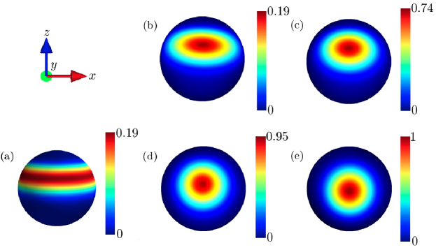
Figure 3: Initial Dicke state under the transformation $e^{-rS_{y}}$. The initial Dicke state $|\psi\rangle=|S=10,m=4\rangle$ (a) is deformed as a function of $\gamma$: In (b) we show the deformation for $\gamma=0$.2, in (c) for $\gamma=0.5$, in (d) for $\gamma=0.9$ and in (e) for $\gamma=0.99$. Interestingly, for $\gamma\approx 1$ the transformation turns a Dicke state into a coherent one.

The dynamics of the system is very different for $\gamma<v$ and $\gamma>v$. On the one hand, when $\gamma>v$, we obtain $\tilde{H}=-2i\,\sqrt{\gamma^{2}-v^{2}}\;S_{z}$ such that

$$U(t)=e^{\alpha\,S_{y}}\;e^{-2\sqrt{\gamma^{2}-v^{2}}\,S_{z}\,t}\;e^{-\alpha\,S_{y}}\;,$$ (18)

with $\alpha={\rm atanh}(v/\gamma)$, real. Thus the evolution operator consists entirely of exponential solutions – i.e. rotations with purely imaginary arguments. Therefore, for sufficiently long times, $U(t)$ maps any initial state $|\Psi_{0}\rangle$ to

$$\lim_{t\to\infty}U(t)\;|\Psi_{0}\rangle\propto e^{\alpha\,S_{y}}\;|S,-S\rangle\;.$$ (19)

On the other hand, for $\gamma<v$, the eigenvalues of $H$ are all real, and the evolution in time consists of rotations around the $z$-axis. For the similarity transformation, we find $\alpha=-i\pi/2+r$, where

$$r={\rm atanh}(\gamma/v)=\frac{1}{2}\,\ln\Big{(}\,\frac{v+\gamma}{v-\gamma}\,\Big{)}\;.$$ (20)

In this way, we arrive at

$$U(t) =e^{-i\pi/2\,S_{y}}\,e^{r\,S_{y}}\;e^{-2i\sqrt{v^{2}-\gamma^{2}}\,S_{z}\,t}\;e^{-r\,S_{y}}\,e^{i\,\pi/2\,S_{y}}$$

$$=e^{r\,S_{y}}\;e^{-2i\sqrt{v^{2}-\gamma^{2}}\,S_{x}\,t}\;e^{-r\,S_{y}}\;.$$ (21)

According to this equation, the evolution of a quantum state consists of a rotation around the $x$-axis, sandwitched between a deformation of the state with the non-unitary operator $e^{-r\,S_{y}}$, and its inverse. In what follows we limit ourselves to this regime ($\gamma<v$), where some unitary dynamics (the rotation) still persists.

In Fig. 3, we show the effect of the deformation operator $e^{-r\,S_{y}}$ when choosing a Dicke state as initial state. For that purpose, we plot the Husimi function of the state before [panel (a)] and after applying the deformation operator. The remaining results are shown in the rest of the panels for increasing values of $\gamma$ (see the figure for details). This deformation changes the norm of the state very strongly, in particular when $\gamma$ comes close to $v$. For that reason we plot the normalized Husimi functions.

Note that for $r$ sufficiently large (i.e. $\gamma$ sufficiently close to $v$), the operator $e^{-rS_{y}}$ will map practically any state onto its eigenstate corresponding to the largest negative eigenvalue. This is a coherent state placed on the $y-$axis. This explains the fact that for increasing value of $\gamma$ [panels (b), (c), (d), (e)] the deformed state becomes ever more similar to the just mentioned coherent state.

3.2 Decomposition method

In the interval $\gamma\in[0,1)$, the spectrum of $H$ is real but the associated eigenfunctions tend to align to each other as $\gamma\rightarrow 1$, i.e. close to the EP. Numerically, this yields inacuracies which we want to avoid. For that purpose, we follow weigert , which allows to disentangle the evolution operator as follows. In general, the disentangling method searches for typically time-dependent coeficients $\alpha,\beta,\gamma$ such that

$$e^{-iHt}=e^{-i\alpha\,S_{1}}\;e^{-i\beta\,S_{2}}\;e^{-i\gamma\,S_{3}}\;.$$ (22)

where the operators $S_{1},S_{2},S_{3}$ are chosen from the angular momentum operators $S_{x},S_{y},S_{z}$. Many different combinations are possible Varshalovichbook , but as long as the dynamics is unitary, one refers to the parameters $\alpha,\beta,\gamma$ as Euler angles. In the present case, however, the dynamics is not unitary and some of the parameters must be complex or imaginary. After considering and discarding the quantum mechanical $S_{z}$–$S_{y}$–$S_{z}$ scheme, as well as the Gauss decomposition scheme Varshalovichbook due to eventual singularities, we found the following decomposition particularly convenient:

$$U(t)=e^{-i\alpha S_{z}}e^{-i\beta\,S_{y}}e^{-ih\,S_{x}}\;.$$ (23)

Deriving both sides of (23) by $t$, and then comparing them (factoring out the evolution operator), using the lineal independence of $S_{x}$, $S_{y}$ and $S_{z}$, one arrives at the following system of differential equations:

$$\dot{\alpha}-\dot{h}\;\sin\beta =-2i\,\gamma$$

$$\dot{\beta}\;\cos\alpha+\dot{h}\;\sin\alpha\;\cos\beta =0$$

$$\dot{\beta}\;\sin\alpha-\dot{h}\;\cos\alpha\;\cos\beta =-2v\;.$$ (24)

This system of equations can be converted into a real system for real parameters $f=i\alpha,g=i\beta,h$ which yields

$$\dot{f} =\tanh(g)\;\cosh(f)\;2v+2\gamma$$

$$\dot{g} =-2v\;\sinh(f)$$

$$\dot{h} =2v\;\frac{\cosh(f)}{\cosh(g)}\;.$$ (25)

The initial condition is $U(0)=\mathbb{1}$, which implies $f(0)=g(0)=h(0)=0$. Therefore, the system of equations has a unique solution, which assures that $f,g,h$ are real functions in time. In principle the system of ordinary differential equations can be solved analytically, by calculating the eigenvalues and eigenstates of the coefficient matrix. For simplicity, however, we have used numerical solutions of Eq. 25 and the results are presented below.

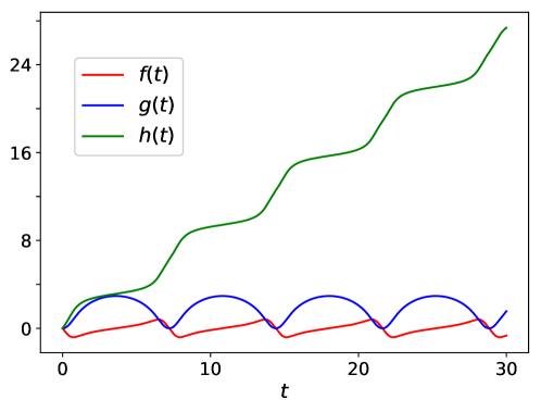
Figure 4: Numerical solutions of Eq. (25) for $v=1$ and $\gamma=0.9$.

In Fig. 4 we show the numerical solutions for these functions, for $v=1$ and $\gamma=0.9$, in a time interval $t\in[0,30]$. The function $h(t)$ (green) represents the way the unitary operator $\exp(-ih(t)S_{x})$ acts on the initial state. This only generates rotations around the $x$-axis on the phase space. Further, $h(t)$ is a monotonously increasing function. On the other hand, $f(t)$ (red) and $g(t)$ (blue) are periodic functions, such that the corresponding evolution operators perform imaginary rotations, which have their origin in the non-unitary part of the Hamiltonian $H$. This will lead to interesting dynamical effects discussed below. The dependence on $\gamma$ is reflected on the slope of $h(t)$ and the periods of $f(t)$ and $g(t)$.

In fact, according to Eqs. (16) and (21) one can see that the evolution is periodic with period $T=\pi/\sqrt{1-\gamma^{2}}$ ($v=1$). This is indeed the period of $f(t)$ and $g(t)$. For the monotone function $h(t)$ and the corresponding operator $\exp(-ih(t)S_{x})$, this means that $h(nT)=2\pi n$, for integer $n$. So, applying a linear fit to $h$ yields the slope $2\sqrt{1-\gamma^{2}}$.

3.3 Time evolution of the quantum state intensity

In our system the norm of a evolving quantum state is not conserved. From the physical point of view such a state may represent a large number of particles in a (may be effective) single particle quantum state (e.g. Bose-Einstein condensate  GraefePRL2008 , or quasi-particles in quantum transport Feng2012 ) or the quantum state can be interpreted as a classical wave field PhysRevLett.86.787 ; RochaPRApp2020 . In any case, the change in the norm squared of the state, i.e. its trace, can be interpreted as the loss or gain of particles or wave field intensity. The term “quantum state intensity” should be understood in this manner.

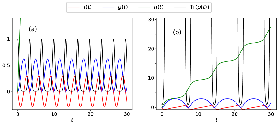
Figure 5: Time evolution of the functions involved in the disentagling of the evolution operator Eq. (23) along with the time evolution of the trace for the initial state $\left|\theta_{0}=\nicefrac{{\pi}}{{2}},\phi_{0}=\nicefrac{{\pi}}{{4}}\right\rangle$; $\sin\phi_{0}\approx 0$.$707$. (a) $\gamma=0.3$, (b) $\gamma=0.9$.

At this point it is instructive to analyze the evolution of the trace of the two different initial states given in the introduction along with the decomposition of the evolution operator, Eq. (23). The intensity of each state oscillates in different ways, which depend on the initial state and also on the value of $\gamma$. If the initial coherent state is centered in the $(S_{x},S_{y})$ plane, i.e. $\theta_{0}=\pi/2$, we observe that, for $\gamma<\sin\phi_{0}$, the trace oscillates in the values $0<\rho(t)\leq 1$. The minimal value that the trace attains depends on the initial state and $\gamma$. Further, the minima of the trace corresponds to the maxima of $g(t)$. These effects are shown in Fig. 5(a) for $\sin\phi_{0}\approx 0$.$707$, and $\gamma=0.3$.

For $\gamma>\sin\phi_{0}$, the trace oscillates between $1\leq\operatorname{Tr}(\rho(t))<M$, for $M>1$, where the maximum value of $M$ can be quite large. (This factor of $\sin\phi_{0}$ emerges when analyzing the evolution in phase space: Sec. 4.1.) In Fig. 5(b) for $\gamma=0.9$, clearly close to the EP, this value of $M$ can be as large as $\sim 10^{9}$. Besides, the minima of the trace corresponds to the minima of $g(t)$. This behaviour is also exhibited for an initial Dicke state with $m=0$, but in contrast to the previous case, it holds for all values of $\gamma$.

If the initial coherent state is not centered in the $xy$ plane, or for initial Dicke states with $m\neq 0$, the trace oscillates between a minimum value (that for some cases can be zero) and a value greater than one, irrespectively of the value of $\gamma$. As in the previous cases, this maximum value can be quite large. This generic behaviour is shown in Fig. 6 for a Dicke state $\left|S=10,m=4\right\rangle$ and $\gamma=0.7$. Further, notice that the minima of the trace do not coincide, though is close, to the minima of $g(t)$ (c.f. Fig. 6).

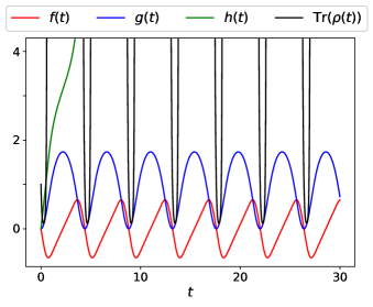
Figure 6: Time evolution of the functions involved in the disentagling of the evolution operator Eq. (23) along with the time evolution of the trace for the initial state $|S=10,m=4\rangle$ and $\gamma=0.7$.

4 Time evolution in phase space

In this section, we consider the evolution of the Husimi distribution and we analyze the evolution of the angular momentum expectation values. In the case of initial coherent states, we find a one-to-one correspondence between the trajectories traced by the expectation values and the characteristics of the evolution equation for the Husimi function. This is due to the fact that coherent states remain coherent during evolution – only their intensity (trace) changes. For initial Dicke states, this is no longer true.

4.1 Time dependent Husimi distribution

We are now in the position to study the time evolution in phase space of the system. Using the decomposition from Eq. (2) of the Hamiltonian into a Hermitian and an anti-Hermitian part, $H=H_{0}+i\Gamma$, the von Neumann equation can be written as

$$i\partial_{t}\rho(t)=[H_{0},\rho(t)]+i[\Gamma,\rho(t)]_{+}.$$ (26)

Following App. B, one gets the equation of motion of the Husimi function

$$i\partial_{t}{Q}(\theta,\phi)=-2(v\hat{l}_{x}+2i\gamma S\cos\theta-i\gamma\sin\theta\partial_{\theta})Q(\theta,\phi),$$ (27)

where $\hat{l}_{x}=i(\sin\phi\partial_{\theta}+\cot\theta\cos\phi\partial_{\phi})$. The method of characteristics then yields

$$\dot{\theta} = -2v\sin\phi+2\gamma\sin\theta,$$ (28)

$$\dot{\phi} = -2v\cot\theta\cos\phi,$$

$$\dot{Q} = 4\gamma S\cos\theta.$$

It is worth noting that the first two equations above are consistent with the Ehrenfest equations derived for coherent states (Sec. 4.2, Eq. (35)) and the last equation describes the deformation of the distribution along the characteristics.

As we have demonstrated in the App. C, the trajectories of the expectation values (in the case of coherent states) or the characteristics of Eq. (28), trace circles in phase space symmetric respect to deflection on the $yz$ plane. This implies that for an initial state with a Husimi function of the same symmetry that this symmetry is conserved. So for instance, as $\left\langle S_{x}\right\rangle=0$ for a Dicke state, $\left\langle S_{x}\right\rangle$ will remain zero for all times (See Fig. 8(b)).

We continue with the analysis of the time evolution of the Husimi function for $\gamma\in[0,1)$ in phase space. We observe that the distribution only spins around for coherent states (though there is an exception which is explained below in this section) but for initial Dicke states beside spinning it deforms too (also see below in this section). As before, the period and amplitude of the rotation depend on the initial state, as well as on the value of $\gamma$. The rotation period is the same as the periods of $f(t)$ and $g(t)$.

An interesting behaviour occurs on the rotating distribution. When it comes closer to the point $\left(\theta=\nicefrac{{\pi}}{{2}},\phi=\nicefrac{{\pi}}{{2}}\right)$, the distribution moves slower than it does on other regions. This also happens with initial Dicke states, but besides the rotation of the distribution, its Husimi function also becomes localized. Fig. 7 shows this effect for an initial Dicke state $|S=10,m=4\rangle$ with $\gamma=0.7$ at $t=2.4$.

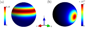
Figure 7: Time evolution of an initial Dicke state in phase space for $\gamma=0.7$. (a) the state $\left|S=10,m=4\right\rangle$. $\gamma=0.7$ at $t=0$. (b) the evolved state at $t=2.4$.

On the other hand, when the Husimi distribution comes closer to the point $(\theta=\nicefrac{{\pi}}{{2}},\phi=-\nicefrac{{\pi}}{{2}})$, while it moves faster for both types of states, also the correspondig distribution of the initial Dicke state recovers its original form.

Another courious effect happens for an initial coherent state located on the plane $(x,y)$. As $\gamma$ gets closer to $\sin\phi_{0}$, the amplitude of the rotations decreases until it becomes zero for $\gamma=\sin\phi_{0}$. For this particular value of $\gamma$ the Husimi function becomes stationary. When $\gamma>\sin\phi_{0}$, the amplitude increases and we recover the spinning pattern. Before and after that value, the distribution moves initially towards different directions, so the center of the circle followed by the distribution can be on one side or the other of the starting point. An explanation for the $\sin\phi_{0}$ factor is given in App. C.

Most of this discussion is then analyzed from another perspective in Sec. 4.2, where it is also illustrated.

4.2 Ehrenfest equations and the time evolution of the expectation values

In order to get an insight of what will be the time evolution of the distributions in phase space, we study the first and second moments of the operators $\{S_{x},S_{y},S_{z}\}$. Denoting for an observable $\hat{A}$, $\mbox{tr}(\,\hat{A}\rho\,)=\langle\langle\hat{A}\rangle\rangle$, we rewrite Eq. (8) as

$$\langle\hat{A}\rangle=\frac{\langle\langle\,\hat{A}\,\rangle\rangle}{{\rm tr}(\rho)}\;.$$ (29)

The evolution of the expectation value of $\hat{A}$ can be obtained from the Ehrenfest equation. However, we have to take into account that the trace of the density matrix depends on time. For a general Hamiltonian with $H=H_{0}+i\Gamma$ with Hermitian operators $H_{0}$ and $\Gamma$ one obtains GraefeJPA2010

$$i\frac{d}{dt}\langle\!\langle A\rangle\!\rangle=\langle\!\langle[A,H_{0}]+i[A,\Gamma]_{+}\rangle\!\rangle.$$ (30)

Writing for the trace of the density matrix ${\rm tr}(\rho)=\langle\langle\mathbb{1}\rangle\rangle$, we obtain

$$\frac{d}{dt}\langle\!\langle\mathbb{1}\rangle\!\rangle=2\,\langle\!\langle\Gamma\rangle\!\rangle$$ (31)

and

$$\frac{d}{dt}\langle A\rangle = \frac{1}{\langle\!\langle\mathbb{1}\rangle\!\rangle}\frac{d}{dt}\langle\!\langle A\rangle\!\rangle-\frac{\langle\!\langle A\rangle\!\rangle}{\langle\!\langle\mathbb{1}\rangle\!\rangle^{2}}\;\frac{d}{dt}\langle\!\langle\mathbb{1}\rangle\!\rangle$$ (32)

$$= \frac{1}{\langle\!\langle\mathbb{1}\rangle\!\rangle}\frac{d}{dt}\langle\!\langle A\rangle\!\rangle-2\,\langle A\rangle\,\langle\Gamma\rangle\;.$$

Applying these equations to the Hamiltonian from Eq. (2), we find for the normalized expectation values

$$\begin{split}\frac{d}{dt}\langle S_{x}\rangle&=-2\gamma\langle[S_{z},S_{x}]_{+}\rangle+4\gamma\langle S_{x}\rangle\langle S_{z}\rangle,\\ \frac{d}{dt}\langle S_{y}\rangle&=-2v\langle S_{z}\rangle-2\gamma\langle[S_{z},S_{y}]_{+}\rangle+4\gamma\langle S_{y}\rangle\langle S_{z}\rangle,\\ \frac{d}{dt}\langle S_{z}\rangle&=2v\langle S_{y}\rangle-4\gamma\langle S^{2}_{z}\rangle+4\gamma\langle S_{z}\rangle^{2}.\end{split}\;$$ (33)

For coherent states, the expectation value of the anti-commutators in Eq. (33) can be simplified using the relation GraefePRL2008 , GraefeJPA2010

$$\langle[S_{i},S_{j}]_{+}\rangle=\left(2-\frac{1}{S}\right)\langle S_{i}\rangle\;\langle S_{j}\rangle+\delta_{ij}\,S\;.$$ (34)

Thereby we obtain

$$\begin{split}\dot{s}_{x}&=2\gamma s_{x}s_{z}/S,\\ \dot{s}_{y}&=-2vs_{z}+2\gamma s_{y}s_{z}/S,\\ \dot{s}_{z}&=2vs_{y}+2\gamma s^{2}_{z}/S-2\gamma S,\end{split}\;$$ (35)

where $s_{j}=\langle S_{j}\rangle$. With the above equations it is easy to show that

$$\frac{d}{dt}\,\big{(}\,s_{x}^{2}+s_{y}^{2}+s_{z}^{2}\,\big{)}=0\;,$$ (36)

which means in particular that a coherent state remains coherent throughout the evolution of the system (see App. A).

The analytical solution for this system of equations is derived in App. C. At the heart of this solution, there is the finding that the trajectories are circles on the sphere, which can be defined as the intersection of the sphere with a plane parallel to the $z$-axis and crossing the $y$-axis at a point $y_{0}/S=v/\gamma>1$. In the $xy$ plane we can therefore draw a line through $(0,y_{0})$ and the starting point of the trajectory and thereby find a second intersection point (of the line with the unit circle). Depending on the size of $\gamma$ this second point may be on one side or on the “other side” of the starting point, which explains the movement of the circle centers as $\gamma$ is increased.

Numerical results.

One way to study the dynamics of the evolution is through the expectation value of $\vec{S}$, or in components $\left(s_{x},s_{y},s_{z}\right)$. Fig. 8 shows the trajectories of Eq. (LABEL:vecS) for the initial coherent state $\left|\theta_{0}=\nicefrac{{\pi}}{{2}},\phi_{0}=\nicefrac{{\pi}}{{4}}\right\rangle$ (a) and for the initial Dicke state $|S=10,m=4\rangle$ (b) for different values of $\gamma$. According to Eq. (36), for an initial coherent state, the time evolution of the expectation value of $\vec{S}$ lies always on the surface of the sphere $\mathbb{S}^{2}$. In this case, it represents the center of the distribution. Toghether with the change of “sides” of the circles, also we see that their radii decrease as $\gamma$ approaches $\sin\phi_{0}$. For completeness we have included on Fig. 8(a) the velocities of the different $\gamma$ trajectories. As stated earlier (Sec. 4.1), the distribution moves faster near the point $\left(\theta=\nicefrac{{\pi}}{{2}},\phi=-\nicefrac{{\pi}}{{2}}\right)$. An explanation for this speed up / slow down effect can be given by analyzing the disentangling functions in Eq. (23). We recall that $h(t)$ is a real function and its effect is precisely the rotation of the distribution. The slope of $h(t)$ defines the velocity for which the distribution rotates. As Fig. 4 shows, we see that when $g(t)$ takes values around its maxima, the local slope of $h(t)$ decreases; when $g(t)$ decreases, the local slope of $h(t)$ is more pronounced.

On the other hand, the corresponding $\vec{s}$ values for the evolution of an initial Dicke state never reach the surface of $\mathbb{S}^{2}$. We see that as $\gamma$ increases, the trajectories get closer to the circle $y^{2}+z^{2}=S^{2}$, though they never exactly reach it.

Additionally, the width of the distribution is given by the variances

$$\Delta^{2}S_{j}\left(t\right)=\left\langle S_{j}^{2}\left(t\right)\right\rangle-\left\langle S_{j}\left(t\right)\right\rangle^{2},$$ (37)

where $j=x,y,z$. We compute the sum of the different variances for the evolution of the initial coherent state $\left|\theta_{0}=\nicefrac{{\pi}}{{2}},\phi_{0}=\nicefrac{{\pi}}{{4}}\right\rangle$ and found

$$\sum_{j}\Delta^{2}S_{j}(t)=S.$$ (38)

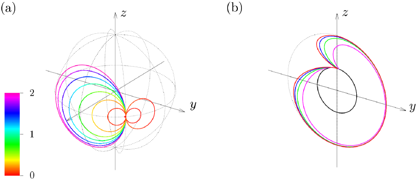
Figure 8: Trajectories of the expectation value of $\vec{S}$ for different values of $\gamma$. In panel (a) for the initial coherent state $\left|\theta=\nicefrac{{\pi}}{{2}},\phi=\nicefrac{{\pi}}{{4}}\right\rangle$, and for $\gamma=0$, $0$.$1$, $\ldots$, $0$.$9$. from left (violet) to right (red). The line color represents the velocity on a common scale from 0 (red) to 2 (violet). In panel (b) for the initial Dicke state $|S=10,m=4\rangle$ for $\gamma=0$ (black solid line), $0.2$ (magenta), $0.4$ (green), $0.6$ (blue), and $0.8$ (red solid line). The dotted line represents the circle $y^{2}+z^{2}=S^{2}$.

Notice that the time evolution of the sum of variances is the same as in the standard coherent state Eq. (48), namely the time evolution leaves invariant (except for the trace) the properties of the initial coherent state.

For initial Dicke states the variances behave differently. We plotted them in Fig. 9 for $|S=10,m=4\rangle$ and $\gamma=0$.$7$. We see that the initial state has variance $\sim S^{2}$, and periodically returns to that value. Interestingly, the sum $\sum_{j}\Delta^{2}S_{j}(t)$ is almost equal to $S=10$ in periodic time intervals. Thus, the sum of fluctuations almost fulfills Eq. (48) and the evolved Dicke state has periodically the properties of a coherent state: for certain periods of time the state attains a pseudo-coherent shape, as in Fig. 7 (though a numerical closer look shows that the sum of fluctuations never reaches exactly the value of $S$).

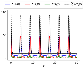
Figure 9: Time evolution of the variances $\Delta^{2}S_{j}(t)$ for the initial Dicke state $|S=10,m=4\rangle$ with $\gamma=0.7$. We also plotted the sum $\sum_{j}\Delta^{2}S_{j}(t)$ and the value $S=10$ (solid black line) for comparison.

As an important final observation, we note that one can obtain a consistent evolution equation for the normalized Husimi function. Defining

$$\rho^{\prime}=\frac{\rho}{\operatorname{tr}\rho}$$ (39)

one gets a modified version of Eq. (26),

$$i\partial_{t}\rho^{\prime}=[H_{0},\rho^{\prime}(t)]+i[\Gamma,\rho^{\prime}(t)]_{+}-i\frac{\rho^{\prime}}{\operatorname{tr}\rho}\frac{d\operatorname{tr}\rho}{dt}.$$ (40)

Using Eq. (31),

$$i\partial_{t}\rho^{\prime}=[H_{0},\rho^{\prime}(t)]+i[\Gamma,\rho^{\prime}(t)]_{+}+4i\gamma\rho^{\prime}\left\langle S_{z}\right\rangle.$$ (41)

Thus for the Husimi function, since $\partial_{t}{Q^{\prime}}(\theta,\phi)=\partial_{t}{Q}_{\rho^{\prime}}(\theta,\phi)$, one obtains

$$\begin{split}\partial_{t}{Q}_{\rho^{\prime}}(\theta,\phi)&=-2(v\hat{l}_{x}+2\gamma S\cos\theta-\gamma\sin\theta\partial_{\theta}\\ &-2i\gamma\rho^{\prime}\left\langle S_{z}\right\rangle)Q^{\prime}(\theta,\phi),\end{split}$$ (42)

which leads to

$$\dot{\theta} = -2v\sin\phi+2\gamma\sin\theta,$$ (43)

$$\dot{\phi} = -2v\cot\theta\cos\phi,$$

$$\dot{Q^{\prime}} = 4\gamma\left(S\cos\theta-\left\langle S_{z}\right\rangle\right).$$

As we pointed out, the evolution of a coherent state remains a coherent state. This is consistent with the latter equation, since in this case,

$$\left\langle S_{z}\right\rangle=S\cos\theta,$$ (44)

therefore

$$\dot{Q^{\prime}}=0.$$ (45)

5 Conclusions

In this contribution we study the time evolution of a quantum system with non-Hermitian, $\mathcal{PT}$-symmetric Hamiltonian with $\operatorname{SO}(3)$ as the dynamical symmetry group, where the corresponding classical phase space is the Bloch sphere. We consider the simplest non-trivial Hamiltonian (linear in the angular momentum operators) and analyze the evolution of, both, the Husimi representation and the evolution of the expectation values of the angular momentum operators.

The system has one single exceptional point (EP), where all eigenstates and eigenvalues coalesce at the same time. Because of this, standard numerical or analytical methods based on the diagonalization of the Hamiltonian quickly become unstable. We overcome this problem by disentangling the evolution operator into three different rotations, two of which are “imaginary”.

In the Hermitian case, the dynamics in phase space would consist of a rigid rotation around a fixed axis. Classical and quantum dynamics would essentially agree, the evolution equation for the Husimi distribution function being equal to the Liouville equation for classical phase space densities. The evolution of expectation values of the angular momentum operators would also agree with the evolution equation of the corresponding classical observables.

For the Hamiltonian studied here, many of these properties do no longer hold. The evolution of the Husimi distribution may still be solved by the method of characteristics, but the system of differential equations which determines the charactersitics is now quadratic and the characteristics themselves are deformed. In addition, the derivative of the Husimi function along these characteristics is no longer constant. Hence, the norm of the evolving quantum state (i.e. its trace) is no longer conserved. The phase space can be divided into the northern hemisphere ($\theta<\pi/2$) which acts as a source and the southern hemisphere ($\theta>\pi/2$) which acts as a sink.

Now, it is no longer possible to derive a closed evolution equation for the above mentioned expectation values. In addition since the Hamiltonian is linear the Planck constant drops out from the Schrödinger equation, so that there is no semiclassical regime, and no valid Ehrenfest equations apparently making it impossible to identify classical trajectories. For instance, studying the evolution of initial Dicke states, we find that the evolution of the angular momentum expectation values is limitted to the $yz$-plane inside the Bloch sphere, while the corresponding evolution for initial coherent states takes place on the Bloch sphere. This makes it possible to find different initial quantum states, such that the trajectories trazed out by the expectation values cross.

Coherent states offer an elegant solution to this problem. As it turns out, these states remain coherent throughout their evolution. Hence the corresponding expectation values trace a trajectory on the Bloch sphere. These trajectories agree with the characteristics and thereby they provide a means to define a corresponding classical dynamical system in a meaningful way. Nevertheless, even a coherent state will suffer from variations of its norm. Hence, the corresponding classical dynamics formulated in terms of the Liouville equation, really describes an ensemble of particles whose size varies according to the particle density function passing over the sources and sinks in phase space.

We have also studied the time evolution under a similarity transformation that effectively diagonalizes the Hamiltonian. In this case the similarity transformation of a coherent state remains coherent, while the similarity transformation of a Dicke state approaches a coherent state (the closer it is, the smaller $v-\gamma>0.9$). After this, the time evolution is a simple rotation around the $x-$axis.

For the present work, the disentangling procedure has been essential and it will be interesting to investigate the possibility to apply that method to PT-symmetric variantes of non-linear models, such as the Kerr or the Lipkin-Meshkov-Glick models valtierra2020quasiprobability .

Appendix A Properties of coherent and Dicke states

We are using as initial states two states with different properties of their distributions: one that is localized and one that is not. In fact, it is well known Klimovbook2009 that for a coherent state $\left|\theta_{0},\phi_{0}\right\rangle$, centered at $\left(\left\langle S_{x}\right\rangle,\left\langle S_{y}\right\rangle,\left\langle S_{z}\right\rangle\right)$ with

$$\left\langle S_{x}\right\rangle = S\sin\theta_{0}\cos\phi_{0},$$

$$\left\langle S_{y}\right\rangle = S\sin\theta_{0}\sin\phi_{0},$$

$$\left\langle S_{z}\right\rangle = S\cos\theta_{0},$$ (46)

its variances are,

$$\Delta^{2}S_{x} = \frac{S}{2}\left(1-\sin^{2}\theta_{0}\cos^{2}\phi_{0}\right),$$

$$\Delta^{2}S_{y} = \frac{S}{2}\left(1-\sin^{2}\theta_{0}\sin^{2}\phi_{0}\right),$$

$$\Delta^{2}S_{z} = \frac{S}{2}\left(1-\cos^{2}\theta_{0}\right),$$ (47)

with the property

$$\Delta^{2}S_{x}+\Delta^{2}S_{y}+\Delta^{2}S_{z}=S.$$ (48)

So the state is localized because its varaiances are $\sim S$.

The Dicke state $\left|S,m\right\rangle$, fulfills

$$\left\langle S_{x}\right\rangle=0,\left\langle S_{y}\right\rangle=0,\left\langle S_{z}\right\rangle=m,$$ (49)

with variances

$$\Delta^{2}S_{x} = \frac{1}{2}\left(S^{2}+S-m^{2}\right),$$

$$\Delta^{2}S_{y} = \frac{1}{2}\left(S^{2}+S-m^{2}\right),$$

$$\Delta^{2}S_{z} = 0,$$ (50)

one can see that the state is not localized, i.e. its variances are $\sim S^{2}$, when $m^{2}\sim S$.

Furthermore, consider the functional,

$$\mathcal{L}\quad:\quad|\Psi\rangle\to\langle S_{x}\rangle^{2}+\langle S_{x}\rangle^{2}+\langle S_{x}\rangle^{2}\;,$$

then we want to show two things: (i) In any case $\mathcal{L}[\Psi]\leq S$; (ii) $\mathcal{L}[\Psi]=S$ if and only if $\Psi$ is a coherent state. Both statements follow rather immediately from the invariance of $\mathcal{L}$ under rotations. For instance to prove (i) assume there exits a $\Psi$ with $\mathcal{L}[\Psi]>S$ then we can find a rotation which makes $\langle S_{x}\rangle=\langle S_{y}\rangle=0$. Hence, we find $\langle S_{z}\rangle>S$ which is impossible because of the eigenvalues of $S_{z}$.

To prove (ii) we note that one direction of the “if and only if” is clear: If $\Psi$ is a coherent state then $\mathcal{L}[\Psi]=S$. To show the other case, assume $\mathcal{L}[\Psi]<S$ and do the rotation just as in the previous case. Then we find $\langle S_{z}\rangle<S$, which means that the state in question cannot be the eigenstate $|S,S\rangle$ which it should be (if $\Psi$ really were a coherent state, according to Eq. (10)).

Appendix B Evolution Equation on Phase Space

The von Neumann equation can be written as

$$i\partial_{t}\rho(t)=[H_{0},\rho(t)]+i[\Gamma,\rho(t)]_{+}.$$ (51)

To recast this equation on phase space, we multiply by the kernel and take the trace

$$i\partial_{t}\mathrm{Tr}\Big{(}\rho(t)\hat{\omega}_{Q}(\theta,\phi)\Big{)} = \mathrm{Tr}\Big{(}[H_{0},\rho(t)]\hat{\omega}_{Q}(\theta,\phi)\Big{)}+$$ (52)

$$i\mathrm{Tr}\Big{(}[\Gamma,\rho(t)]_{+}\hat{\omega}_{Q}(\theta,\phi)\Big{)}.$$

The correspondence rules or Bopp operators are very useful ZFG ; ACGT ; Klimovbook2009 :

$$\left.\hat{\rho}\hat{S}_{z}\atop\hat{S}_{z}\hat{\rho}\right\}\longleftrightarrow\left\{\Big{(}\mp\frac{1}{2}l_{z}+\Lambda_{0}(\theta,\phi)\right.\Big{)}\hat{\rho},$$ (53)

$$\left.\hat{\rho}\hat{S}_{\pm}\atop\hat{S}_{\pm}\hat{\rho}\right\}\longleftrightarrow\left\{\Big{(}\mp\frac{1}{2}l_{\pm}+\Lambda_{\pm}(\theta,\phi)\right.\Big{)}\hat{\rho},$$ (54)

where $l_{\pm,z}$ are the first order differential operators,

$$l_{\pm}=e^{\pm i\phi}\left(\pm\partial_{\theta}+i\mathrm{cot}\theta\partial_{\phi}\right),\quad l_{z}=-i\partial_{\phi}.$$ (55)

The operators $\Lambda_{0,\pm}(\theta,\phi)$ are

$$\Lambda_{0}(\theta,\phi)=\frac{1}{2}\left(\frac{1}{\epsilon}\cos\theta-\cos\theta-\sin\theta\partial_{\theta}\right),$$ (56)

$$\Lambda_{\pm}(\theta,\phi)=\frac{e^{\pm i\phi}}{2\epsilon}\pm\frac{1}{2}\Big{[}\cos\theta l_{\pm}-e^{\pm i\phi}\sin\theta(l_{z}\pm 1)\Big{]},$$ (57)

with $\epsilon=(2S+1)^{-1}$.

Using Eqs. (53) and (54), Eq. (52) takes the following form

$$i\partial_{t}Q(\theta,\phi)=-2\left(vl_{x}+2i\gamma S\cos\theta-i\gamma\sin\theta\partial_{\theta}\right)Q(\theta,\phi).$$ (58)

Another way to obtain Eq. (58) is through KlimovJMP2002 . Eq. (52), can be recasted in the following form

$$i\partial_{t}Q(\theta,\phi)=\frac{i}{S}\{Q(\theta,\phi),Q_{H_{0}}(\theta,\phi)\}_{p}+i\ \hat{\Xi}(\theta,\phi)Q(\theta,\phi).$$ (59)

Here

$$\{F,G\}_{p}=\frac{1}{\sin\theta}\left(\partial_{\phi}F\ \partial_{\theta}G-\partial_{\theta}F\ \partial_{\phi}G\right)$$ (60)

are the Poisson brackets on the sphere and

$$\hat{\Xi}(\theta,\phi)Q(\theta,\phi)=\operatorname{Tr}([\Gamma,\rho(t)]_{+}\hat{\omega}_{Q}\left(\theta,\phi\right))$$ (61)

is the corresponding action of the anticommutator of $\Gamma$ and the density matrix on $Q$.

The structure of Eq. (59) comprises a sympletic structure given by the Possion brackets $\{,\}_{p}$ plus a term which originates from the $\mathcal{PT}$-symmetric structure of the Hamiltonian. This structure is similar to the one found by Graefe and coworkers in GraefeJPA2010 .

Appendix C Analytical solution of the Ehrenfest Equations for coherent states

According to Eq. (35), let $x$, $y$ and $z$ be $s_{x}/S$, $s_{y}/S$ and $s_{z}/S$, respectively. Then we get the system of equations,

$$\dot{x} = 2\gamma xz$$

$$\dot{y} = -2vz+2\gamma yz$$

$$\dot{z} = 2vy+2\gamma z^{2}-2\gamma,$$ (62)

valid for the evolution of coherent states. Our aim is it to find the trajectories on the sphere. First, we divide the second equation by the first and obtain

$$\frac{dy}{dx}=y^{\prime}(x)=\left(y-\frac{v}{\gamma}\right)\frac{1}{x}\ \Longrightarrow\ y(x)=C_{1}x+\frac{v}{\gamma}.$$ (63)

Here $C_{1}$ is a first integration constant, which is determined from the initial conditions and yields

$$C_{1}=-\frac{v/\gamma-y_{0}}{x0}=-\frac{v/\gamma-\sin\theta_{0}\sin\phi_{0}}{\sin\theta_{0}\cos\phi_{0}},$$ (64)

where $\theta_{0}$ and $\phi_{0}$ are the parameters of the initial coherent state. Now we simply use the fact that (Eq. (36))

$$x^{2}+y^{2}+z^{2}=1.$$ (65)

This means tha the trajectory is just the intersection of the unit sphere with the plane. This always gives a circle, with its center in the $(x,y)$ plane. Let $(x_{c},y_{c})$ be the center of that circle and $(\Delta x,\Delta y)$ be such that

$$\vec{r}(\alpha)=\left(\begin{array}[]{c}x_{c}\\ y_{c}\\ 0\end{array}\right)+\left(\begin{array}[]{c}\Delta x\\ \Delta y\\ 0\end{array}\right)\cos\alpha+\left(\begin{array}[]{c}0\\ 0\\ \sqrt{\Delta x^{2}+\Delta y^{2}}\end{array}\right)\sin\alpha.$$ (66)

Then we can calculate all the unknowns $x_{c}$, $y_{c}$, $\Delta x$ and $\Delta y$ from the two intersection points, $x_{1,2}$, of the line $y=C_{1}x+v/\gamma$ and the circle $x^{2}+y^{2}=1$ in the $(x,y)$ plane:

$$x^{2}+\left(C_{1}x+v/\gamma\right)^{2}=1,$$ (67)

then

$$x_{1,2} = -p\pm\sqrt{p^{2}-q},$$

$$p = \frac{v}{\gamma}\frac{C_{1}}{1+C_{1}^{2}},$$

$$q = \frac{v^{2}/\gamma^{2}-1}{1+C_{1}^{2}}.$$ (68)

With this we obtain

$$x_{c} = \frac{x_{1}+x_{2}}{2}=-p,$$

$$y_{c} = C_{1}x_{c}+v/\gamma=-C_{1}p+v/\gamma,$$ (69)

and also

$$\Delta x = \frac{x_{1}-x_{2}}{2}=\sqrt{p^{2}-q},$$

$$\Delta y = C_{1}\Delta x=C_{1}\sqrt{p^{2}-q}.$$ (70)

Now, as we observed some trajectories that degenerated to a point, let us find a solution for

$$\Delta x = \Delta y=0$$

$$\Delta z = \sqrt{\Delta x^{2}+\Delta y^{2}}=0.$$ (71)

It is clear from Eq. (70) that this is fulfilled when $p^{2}=q$, which yields

$$\gamma=\frac{\pm i\cos\theta_{0}\cos\phi_{0}+\sin\phi_{0}}{\sin\theta_{0}}v.$$ (72)

We see that real solutions exist only for $\theta_{0}=\pi/2$. Only the trajectory of the evolution of an initial coherent state located on the $(x,y)$ plane degenerates to a point. The value of $\gamma$ that leads to this is ($v=1$)

$$\gamma=\sin\phi_{0}.$$ (73)

Furthermore, in this case ($\theta_{0}=\pi/2$, $v=1$) we have

$$x_{c}-x_{0} \sim \sin\phi-\gamma,$$

$$y_{c}-y_{0} \sim \sin\phi-\gamma,$$ (74)

so both, $x_{c}-x_{0}$ and $y_{c}-y_{0}$, suffer a change of sign before and after Eq. (73). This means that trajectories for $\gamma<\sin\phi_{0}$ and for $\gamma>\sin\phi_{0}$ are centered in different sides of the common point ($\theta_{0},\phi_{0}$). All this is exemplified in Fig. 8.

Acknowledgements

The authors are grateful to A. B. Klimov for many fruitful discussions. T.G. received financial support from CONACyT through the grant “Ciencia de Frontera 2019”, No. 10872.

Appendix D Declarations

Funding

CONACyT “Ciencia de Frontera 2019”, Number 10872.

Conflict of interest

The authors declare that they have no conflict of interest.

Availability of data and material

The data generated for the paper are available upon personal request to the authors.

Code availability

The numerical programs are available upon personal request to the authors.

Authors’ contributions

All authors have contributed equally to the research.

References

- (1) C. M. Bender, P. E. Dorey, C. Dunning, D. W. Hook, A. Fring, H. F. Jones, S. Kuzhel, G. Léval, and R. Tateo: PT Symmetry:In Quantum and Classical Physics, 468. World Scientific Publishing Company, Europe (2018)
- (2) C. M. Bender and S. Boettcher: Real Spectra in Non-Hermitian Hamiltonians Having Symmetry, Phys. Rev. Lett. 80, 5243 (1998)
- (3) W. D. Heiss: The physics of exceptional points, J. Phys. A: Math. Theor. 45, 44016 (2012)
- (4) C. M. Bender: PT-symmetric quantum theory, Journal of Physics: Conference Series, 631 012002 (2015)
- (5) L. Feng, R. El-Ganainy, and L. Ge: Non-Hermitian photonics based on parity-time symmetry, Nature 11, 752 (2017)
- (6) R. El-Ganainy, K. G. Makris, M. Khajavikhan, Z. H. Musslimani, S. Rotter, and D. N. Christodoulides: Non-Hermitian physics and PT symmetry, Nature 14, 11 (2018)
- (7) M.-A. Miri and A. Alù: Exceptional points in optics and photonics, Science 363, eaar7709 (2019)
- (8) T. Kato: Perturbation Theory for Linear Operators 2nd ed. 623. Springer, New York (1995)
- (9) C. Dembowski, H.-D. Gräf, H. L. Harney, A. Heine, W. D. Heiss, H. Rehfeld, and A. Richter: Experimental Observation of the Topological Structure of Exceptional Points, Phys. Rev. Lett. 86, 787 (2001)
- (10) A. A. Mailybaev, O. N. Kirillov, and A. P. Seyranian: Geometric phase around exceptional points, Phys. Rev. A 72, 014104 (2005)
- (11) B. Peng, S. K. Özdemir, M. Liertzer, W. Chen, J. Kramer, H. Yılmaz, J. Wiersig, S. Rotter, and L. Yang: Chiral modes and directional lasing at exceptional points, PNAS 113, 6845 (2016)
- (12) A. Regensburger, C. Bersch, M.-A. Miri, G. Onishchukov, D. N. Christodoulides, and U. Peschel: Parity-time synthetic photonic lattices, Nature 488, 167 (2012)
- (13) Z. Lin, H. Ramezani, T. Eichelkraut, T. Kottos, H. Cao, and D. N. Christodoulides: Unidirectional Invisibility Induced by Symmetric Periodic Structures, Phys. Rev. Lett. 106, 213901 (2011)
- (14) L. Feng, Y.-L. Xu, W. S. Fegadolli, M.-H. Lu, J. E. B. Oliveira, V. R. Almeida, Y.-F. Chen, and A. Scherer: Experimental demonstration of a unidirectional reflectionless parity-time metamaterial at optical frequencies, Nat. Mater. 12, 108 (2012)
- (15) W. Chen, S. K. Özdemir, G. Zhao, J. Wiersig, and L. Yang: Exceptional points enhance sensing in an optical microcavity, Nature 548, 192 (2017)
- (16) T. Goldzak, A. A. Mailybaev, and N. Moiseyev: Light Stops at Exceptional Points, Phys. Rev. Lett. 120, 013901 (2018)
- (17) L. Jin and Z. Song: Solutions of symmetric tight-binding chain and its equivalent Hermitian counterpart, Phys. Rev. A 80, 052107 (2009)
- (18) Y. N. Joglekar, D. Scott, M. Babbey, and A. Saxena: Robust and fragile symmetric phases in a tight-binding chain, Phys. Rev. A 82, 030103 (2010)
- (19) A. Ortega, T. Stegman, L. Benet, and H. Larralde: Spectral and transport properties of a -symmetric tight-binding chain with gain and loss, J. Phys. A: Math. Theor. 53, 445308 (2020)
- (20) E. M. Graefe, M. Höning, and H. J. Korsch: Classical limit of non-Hermitian quantum dynamics-a generalized canonical structure, J. Phys. A: Math. Theor. 43, 075306 (2010)
- (21) E. M. Graefe and R. Schubert: Wave-packet evolution in non-Hermitian quantum systems, Phys. Rev. A 83, 060101 (2011)
- (22) L. Praxmeyer, P. Yang, and R.-K. Lee: Phase-space representation of a non-Hermitian system with symmetry, Phys. Rev. A 93, 042122 (2016)
- (23) E. M. Graefe, H. J. Korsch, and A. E. Niederle: Quantum-classical correspondence for a non-Hermitian Bose-Hubbard dimer, Phys. Rev. A, 82, 013629 (2010)
- (24) S. Mudute-Ndumbe and E. M. Graefe: A non-Hermitian symmetric kicked top, New J. Phys., 22, 103011 (2020)
- (25) R. J Glauber: Coherent and incoherent states of the radiation field, Phys. Rev. 131, 2766 (1963)
- (26) E. C. G. Sudarshan: Equivalence of Semiclassical and Quantum Mechanical Descriptions of Statistical Light Beams, Phys. Rev. Lett. 10, 277 (1963)
- (27) E. P. Wigner: On the quantum correction for thermodynamic equilibrium, Phys. Rev. 40, 749 (1932)
- (28) K. Husimi: Some formal properties of the density matrix, Proc. Phys. Math. Soc. Jpn. 22, 264 (1940)
- (29) E. M. Graefe, H. J. Korsch, and A. E. Niederle: Mean-Field Dynamics of a Non-Hermitian Bose-Hubbard Dimer, Phys. Rev. Lett. 101, 150408 (2008)
- (30) K. Jones-Smith and H. Mathur: Non-Hermitian quantum Hamiltonian with symmetry. Phys. Rev. A, 82, 042101 (2010)
- (31) H. Weyl: Gruppentheorie und Quantemechanik 1st ed. 46. Hirzel-Verlag, Lepizig (1928)
- (32) R. L. Stratonovich: On Distributions in Representation Space, JETP 31, 1012 (1956)
- (33) J. E. Moyal: Quantum mechanics as a statistical theory, Proc. Camb. Phil. Soc. 45, 99 (1949)
- (34) A. Perelomov: Generalized Coherent States and their Applications. Springer, Berlin (1986).
- (35) D. Varshalovich, A. N. Moskalev, and V. K. Khersonskii: Quantum Theory of Angular Momentum 1st ed. 528. World Scientific, Singapore (1989)
- (36) E. M. Graefe, U. Günther, H. J. Korsch, and A. E. Niederle: The Dissipative Bose-Hubbard Model. Methods and Examples, J. Phys. A: Math. Theor. 41, 255206 (2008)
- (37) S. Wiegert: Baker-Campbell-Hausdorff relation for special unitary groups SU(N), J. Phys. A 30, 8739 (1997)
- (38) V. Domínguez-Rocha, R. Thevamaran, F. Ellis, and T. Kottos: Environmentally Induced Exceptional Points in Elastodynamics, Phys. Rev. Applied 13, 014060 (2020)
- (39) A. B. Klimov: Exact evolution equations for SU(2) quasidistribution functions, J. Math. Phys. 43, 2202 (2002)
- (40) I. F. Valtierra, A. B. Klimov, G. Leuchs, and L. L. Sánchez-Soto: Quasiprobability currents on the sphere, Phys. Rev. A 101 033803 (2020)
- (41) A. B. Klimov and S. M. Chumakov: A Group-Theoretical Approach to Quantum Optics, 322. Wiley-VCH, Weinheim (2009)
- (42) W. M. Zhang, D. H. Feng, and R. Gilmore: Coherent states: Theory and some applications, Rev.Mod. Phys. 62 867 (1990)
- (43) F. T. Arecchi, E. Courtens, R. Gilmore, and H. Thomas: Atomic Coherent States in Quantum Optics, Phys. Rev. A 6 2211 (1972)