The Langevin Noise Approach for Lossy Media and the Lossless Limit

Abstract

The Langevin noise approach for quantization of macroscopic electromagnetics for three-dimensional, inhomogeneous environments is compared with normal mode quantization. Recent works on the applicability of the method are discussed, and several examples are provided showing that for closed systems the Langevin noise approach reduces to the usual cavity mode expansion method when loss is eliminated.

I Introduction

Methods for the study of the quantum properties of light, and the interaction of quantized light and atoms and other multi-leveled systems, were initially developed for vacuum. The observation of Purcell in 1946 that the spontaneous emission rate of an atom was dependent on the atom’s environment Purcell was a motivating factor for the study of how cavity materials affect quantized light. The incorporation of simplified models of materials (lossless, dispersionless dielectrics, perfect metals) is accommodated in quantum models in a fairy straightforward manner DM . However, the Kramers-Kronig relations Jac require that absorption is always accomplished by dispersion, and vice versa. Whereas in classical electromagnetics, dispersion and absorption are easily accounted for, in macroscopic quantum models this is not the case, since a naive implementation of absorption causes the commutators to vanish at long times, violating the Heisenberg uncertainty principle.

Motivated by the fluctuation–dissipation theorem, HB -B2 —describe macroscopic quantum electrodynamics (QED) as inspired by its nature as the quantum version of classical macroscopic electrodynamics—is a phenomenological dipolar, fully quantum, macroscopic theory developed to accommodate lossy, dispersive materials and open environments. It has been widely applied to a variety of problems since it is expressed in terms of the Green function, and allows for very general media, including anisotropic, nonreciprocal, and nonlocal materials Buh , RSW -Force2 . For inhomogeneous, complex-shaped regions, the Green function can be computed numerically Cole . In Ref. Phil , the phenomenological assumptions are derived from a canonical formulation; this approach was later extended to moving media Horsley12 . The equivalence of the approach with an alternative based on auxiliary fields 0710 was demonstrated explicitly 0711 . A critical assessment is provided in AD (see also AD1 )-AD2 ), where a comparison with a generalized Huttner-Barnett approach HB (canonical quantization of a bath of oscillators, based on Hop ) is discussed. Dissipation and dielectric models are also discussed in a wide range of other works, see e.g. Chew .

In AD , the practical equivalence of the Langevin noise approach (LNA) and Huttner-Barnett descriptions is shown. More precisely, it is shown that in an open system, the material oscillator degrees of freedom included in the standard Langevin noise approach must be augmented by quantized photonic degrees of freedom associated with fluctuating fields coming from infinity and scattered by the inhomogeneities of the medium. If space is considered to consist of a uniform background having some small absorption, the free fields coming from infinity are absorbed and the standard Langevin noise approach applies. However, it is often of interest to model finite regions of space having nonabsorbing materials. In AD a scheme is developed considering a finite region of space (which may be vacuum), surrounded by a weakly absorbing/dispersive medium $\varepsilon_{\text{inf}}$ that extends to infinity, and fluctuating polarization currents in $\varepsilon_{\text{inf}}$ generate the missing free fields, in which case the Huttner-Barnett and Langevin noise approaches are shown to be equivalent.

Nevertheless, questions about the validity of the Langevin noise approach remain DLGJ -DGJ , particularly, concerning various limiting procedures such as assuming the material region of interest shrinks to zero, or the limit of a lossless material is taken. In this work, we compare the Langevin noise approach with the standard cavity normal mode approach, which we refer to as normal-mode QED (NMQED) in the following, which is valid for media characterized by Hermitian permittivity tensors (lossless, and therefore, nondispersive). Although it is known that the Langevin noise approach recovers various quantities correctly, such as the atomic spontaneous decay rate, here we show for several explicit examples that the Langevin noise approach results in exactly the same formulation (final equations) as the normal-mode QED, although the former allows for much more general materials than the latter. Several possible geometries may be envisioned: 1) finite-size, PEC-wall cavities (i.e., closed systems) containing lossless inhomogeneous media, 2) same as (1) but for lossy, dispersive media, 3) large-cavity limit cavities containing lossless inhomogeneous media, 4) same as (3) but for lossy inhomogeneous media, 5) open systems, which admit loss even when the materials themselves are lossless. Cases (3) and (4) are actually subsets of (1) and (2); in the former, plane-wave eigenfunctions are used, whereas in the latter, more general cavity eigenfunctions are used. For (1), normal-mode QED is standard, often with homogeneous media (e.g., vacuum). The Langevin noise approach does not apply to Case (1) directly, but can be applied to Case (2), the lossy version. Here, we show that the Langevin noise approach recovers exactly the normal-mode QED equations for several problems considered in the lossless limit (i.e., as Case (2) reduces to Case (1)). For Case (3), the normal-mode QED is often used for homogeneous environments (utilizing discrete plane-wave mode functions to represent the actual mode continuum). Again, the Langevin noise approach can not be applied directly to Case (3), although it applies to Case (4) and again recovers the normal-mode QED result in the lossless limit. In fact, the resulting equations from the Langevin noise approach, e.g., the density operator or population evolution, are easily converted to the normal-mode QED (and, sometimes, vice-versa) using a simple Green function relation. For the study of non-absorbing materials, we point out the need to retain dissipation in the Langevin noise approach model until the final steps of the calculation, at which point the lossless limit can be taken. Similarly, if, say, the medium inhomogeneities vanish (e.g., the structure of interest, such as a metal resonator, shrinks to zero size), that limit must be taken at the end of the development.

Open systems, case (5), cannot be modeled using cavity normal modes, but it can be modeled using Langevin noise approach (in the references cited above, it is inherently a system-bath approach). For open systems, a quasinormal mode quantization (also based on a Langevin noise model) is a useful and natural approach for arbitrarily lossy open system modes SH1 , and implements a formulation akin to the standard modal approach, but for open lossy systems. An advantage of quasinormal modes beyond the Langevin noise approach is to explore nonlinear quantum optics at the system level, where it is no longer valid to treat the medium as a bath, e.g. SH2 –SH3 .

II Basic Relations

We first consider an environment/reservoir such as a three-dimensional cavity $\Omega\subseteq\mathbb{R}^{3}$ with closed surface $\Sigma$, having a uniform background material characterized by $\varepsilon_{\text{bulk}}$ and containing a region $\Omega_{1}\subseteq\Omega$ inhomogeneously-filled with material characterized by relative permittivity tensor $\mathbf{\varepsilon}_{1}\left(\mathbf{r},\omega\right)$ (this could be, e.g., a plasmonic material). The permittivity for all $\mathbf{r}\in\Omega$ is $\mathbf{\varepsilon}\left(\mathbf{r},\omega\right)$. We will assume the magnetic permeability is the unity tensor, although including a permeability response does not change the presented conclusions. As the notation indicates, we can allow $\Omega_{1}=\Omega$, and $\Omega$ can be finite (e.g., a closed system with surface $\Sigma$ perfectly conducting), or in the large-cavity limit. The geometry is depicted in Fig. 1, including a two-level system located somewhere within $\Omega$. We compare two formulations.

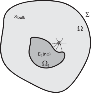
Figure 1: Two-level system in the vicinity of an inhomogeneous region $\Omega_{1}\subseteq\Omega\subseteq\mathbb{R}^{3}$

II.1 Normal-Mode QED Approach

Normal-mode QED is the usual textbook QOB1 -QOB4 and research RA1 -RA2 approach for i) closed empty cavities, where $\mathbf{\varepsilon}\left(\mathbf{r},\omega\right)=\mathbf{I}$, with $\mathbf{I}$ the identity operator, ii) closed cavities filled with lossless, dispersionless media, where $\mathbf{\varepsilon}\left(\mathbf{r}\right)$ is a real-valued, Hermitian tensor, and iii) closed cavities homogeneously-filled with lossy media. For the first two cases, classical mode functions $\mathbf{E}_{\mathbf{k}}\left(\mathbf{r}\right)=\mathbf{E}_{\mathbf{k}}\left(\mathbf{r},\omega_{\mathbf{k}}\right)$ can be defined that satisfy VanB , Wubs2

$$\nabla\times\nabla\times\mathbf{E}_{\mathbf{k}}\left(\mathbf{r},\omega_{\mathbf{k}}\right)=\frac{\omega_{\mathbf{k}}^{2}}{c^{2}}\mathbf{\varepsilon}\left(\mathbf{r}\right)\cdot\mathbf{E}_{\mathbf{k}}\left(\mathbf{r},\omega_{\mathbf{k}}\right),$$ (1)

subject to boundary conditions on the cavity walls, $\left.\widehat{\mathbf{n}}\left(\mathbf{r}\right)\times\mathbf{E}_{\mathbf{k}}\left(\mathbf{r},\omega_{\mathbf{k}}\right)\right|_{\mathbf{r}_{\text{wall}}}=\mathbf{0}$, $\widehat{\mathbf{n}}$ being the unit normal vector to the wall, with eigenfunction orthogonality VanB

$$\int\mathbf{E}_{\mathbf{k}}^{\ast}\left(\mathbf{r},\omega_{\mathbf{k}}\right)\cdot\mathbf{\varepsilon}\left(\mathbf{r}\right)\cdot\mathbf{E}_{\mathbf{k}^{\prime}}\left(\mathbf{r},\omega_{\mathbf{k}^{\prime}}\right)d^{3}\mathbf{r}=\delta_{\mathbf{kk}^{\prime}}.$$ (2)

Under the restriction of a Hermitian permittivity tensor, and defining the Hilbert space of Lebesgue integrable vector functions $\mathbf{L}^{2}$, the operator $L_{E}:\mathbf{L}^{2}\left(\Omega\right)^{3}\rightarrow\mathbf{L}^{2}\left(\Omega\right)^{3}$, $L_{E}\mathbf{x}\equiv\mathbf{\nabla\,\times\,\nabla}\times\mathbf{x}-\frac{\omega_{\mathbf{k}}^{2}}{c^{2}}\mathbf{\varepsilon}(\mathbf{r})\cdot\mathbf{x}$, with boundary condition $B\left(\mathbf{x}\right)=\left.\mathbf{n\times x}\right|_{\Gamma}\mathbf{=0}$ or $B\left(\mathbf{x}\right)=\left.\mathbf{n\times\nabla\times x}\right|_{\Gamma}\mathbf{=0}$ is self adjoint (SA) and negative-definite, and the modes form an orthonormal, complete set in the Hilbert space of square-integrable functions VanB ,

$$\mathbf{I}\delta\left(\mathbf{r}-\mathbf{r}^{\prime}\right)={\displaystyle\sum\nolimits_{\mathbf{k}}}\mathbf{E}_{\mathbf{k}}\left(\mathbf{r},\omega_{\mathbf{k}}\right)\mathbf{E}_{\mathbf{k}}^{\ast}\left(\mathbf{r}^{\prime},\omega_{\mathbf{k}}\right)\cdot\mathbf{\varepsilon}\left(\mathbf{r}^{\prime}\right).$$ (3)

The electric field operator in the Schrödinger picture is

$$\widehat{\mathbf{E}}\left(\mathbf{r}\right)^{\text{NMQED}}={\displaystyle\sum\nolimits_{\mathbf{k}}}\widehat{\mathbf{E}}_{\mathbf{k}}\left(\mathbf{r}\right)+\text{H.c.},$$ (4)

where

$$\widehat{\mathbf{E}}_{\mathbf{k}}\left(\mathbf{r}\right)=i\sqrt{\frac{\hslash\omega_{\mathbf{k}}}{2\varepsilon_{0}}}\widehat{a}_{\mathbf{k}}\mathbf{E}_{\mathbf{k}}\left(\mathbf{r}\right)$$ (5)

and where $\widehat{a}_{\mathbf{k}},\widehat{a}_{\mathbf{k}}^{{\dagger}}$ are annihilation and creation operators that satisfy

$$\left[\widehat{a}_{\mathbf{k}},\widehat{a}_{\mathbf{k}^{\prime}}\right]=\left[\widehat{a}_{\mathbf{k}}^{\dagger},\widehat{a}_{\mathbf{k}^{\prime}}^{\dagger}\right]=0,\ \left[\widehat{a}_{\mathbf{k}},\widehat{a}_{\mathbf{k}^{\prime}}^{\dagger}\right]=\delta_{\mathbf{kk}^{\prime}}.$$ (6)

In the Heisenberg picture, (6) become equal-time commutators.

The free-field Hamiltonian is (dropping the zero-point energy)

$$\widehat{H}^{\text{NMQED}}={\displaystyle\sum\nolimits_{\mathbf{k}s}}\hslash\omega_{\mathbf{k}}\widehat{a}_{\mathbf{k}s}^{\dagger}\widehat{a}_{\mathbf{k}s},$$ (7)

and eigenfunctions of the Hamiltonian are the multimode number (Fock) states

$$\left|n_{1}\right\rangle\left|n_{2}\right\rangle\left|n_{3}...\right\rangle\equiv\left|n_{1},n_{2},n_{3}...\right\rangle=\left|\left\{n_{j}\right\}\right\rangle,$$ (8)

which can be obtained from the ground state as

$$\left|n_{1}\right\rangle\left|n_{2}\right\rangle...n_{i},...=\frac{\left(\widehat{a}_{1}^{\dagger}\right)^{n_{1}}}{\sqrt{n_{1}!}}...\frac{\left(\widehat{a}_{i}^{\dagger}\right)^{n_{i}}}{\sqrt{n_{i}!}}...\left|0\right\rangle.$$ (9)

For the special case of an optically large vacuum cavity, the cavity mode functions become

$$\mathbf{E}_{\mathbf{ks}}\left(\mathbf{r}\right)\rightarrow\frac{\mathbf{e}_{\mathbf{k}s}}{\sqrt{V}}e^{i\mathbf{k}\cdot\mathbf{r}},$$ (10)

which satisfy periodic boundary conditions ($\Omega$ is assumed to be the union of boxes of volume $V$), where $s$ indicates spin (polarization), with $\mathbf{e}_{\mathbf{k}s}$ being an orthonormal set of polarization functions such that $\mathbf{e}_{\mathbf{k}s}\cdot\mathbf{e}_{\mathbf{k}^{\prime}s^{\prime}}=\delta_{\mathbf{kk}^{\prime}}\delta_{ss^{\prime}}$, and satisfy the transversality condition $\mathbf{k}\cdot\mathbf{e}_{\mathbf{k}s}=0$. The polarization vectors form a right-handed coordinate system, $\mathbf{e}_{\mathbf{k}1}\times\mathbf{e}_{\mathbf{k}2}=\mathbf{k/\left|\mathbf{k}\right|}$. In (10), $V$ is a quantization volume such that

$$\int_{V}\mathbf{E}_{\mathbf{ks}}^{\ast}\left(\mathbf{r}\right)\cdot\mathbf{E}_{\mathbf{k}^{\prime}s^{\prime}}\left(\mathbf{r}\right)d^{3}\mathbf{r}=\delta_{\mathbf{kk}^{\prime}}\delta_{ss^{\prime}}.$$ (11)

Note, however, that this is not an open system (truly infinite space), which inherently allows dissipation (photons going to infinity and never coming back). Mathematically, the difference between a large cavity and a true open system is that for the latter, modes must satisfy the Sommerfeld radiation condition, which renders the operator $L_{E}$ to be non-self-adjoint; the Sommerfeld radiation condition is an out-going wave condition, and the adjoint condition is an inward-traveling wave.

Finally, for case (iii), a cavity homogeneously-filled with lossy media, rather than $L_{E}$, the operator $L\mathbf{x}\equiv\mathbf{\nabla\,\times\,\nabla}\times\mathbf{x}$ can be defined such that eigenfunctions of $L$ satisfy the boundary condition $B\left(\mathbf{x}\right)=\mathbf{0}$, and the resulting operator is SA. The cavity must be homogeneously-filled; material inhomogeneities in piecewise constant media would necessitate boundary conditions $B$ such that $B\neq B^{\ast}$, rendering the problem non-self-adjoint.

In the usual normal-mode QED, the photonic Green functions is not explicitly needed, although it implicitly arises in, e.g., atom-atom coupling terms. However, to make connection with the Langevin noise approach, it is important to connect the mode functions $\mathbf{E}_{\mathbf{k}}\left(\mathbf{r},\omega_{\mathbf{k}}\right)$ with the Green tensor, which is defined by

$$\nabla\times\nabla\times\mathbf{G}\left(\mathbf{r},\mathbf{r}^{\prime},\omega\right)-\frac{\omega_{\mathbf{k}}^{2}}{c^{2}}\mathbf{\varepsilon}\left(\mathbf{r}\right)\cdot\mathbf{G}\left(\mathbf{r},\mathbf{r}^{\prime},\omega\right)=\mathbf{I}\delta\left(\mathbf{r}-\mathbf{r}^{\prime}\right)$$ (12)

and satisfies $\mathbf{G(r},\mathbf{r}^{\prime}\mathbf{)}^{\top}=\mathbf{G(r}^{\prime},\mathbf{r)}$. The Green tensor can be expanded as

$$\mathbf{G}\left(\mathbf{r},\mathbf{r}^{\prime},\omega\right)={\displaystyle\sum\nolimits_{\mathbf{k}}}c^{2}\frac{\mathbf{E}_{\mathbf{k}}\left(\mathbf{r},\omega_{\mathbf{k}}\right)\mathbf{E}_{\mathbf{k}}^{\ast}\left(\mathbf{r}^{\prime},\omega_{\mathbf{k}}\right)}{\omega_{\mathbf{k}}^{2}-\omega^{2}}.$$ (13)

The expression (13) formally encompasses the case of transverse modes, forming a transverse Green function, or could include longitudinal modes as well. It should be emphasized that (13) is only valid for closed cavities and the three cases discussed, although the Green tensor concept itself extends to dispersive and lossy inhomogeneous media. For certain spatial positions, a quasinormal mode expansion of the Green function is also possible SH1 –SH2 .

An important expression relating the Green function and modal summation is obtained by integrating (13) with respect to frequency and using the Sokhotski–Plemelj (SP) identity

$$\lim_{\varepsilon\rightarrow 0^{+}}\frac{1}{x\pm i\varepsilon}=\text{PV}\left(\frac{1}{x}\right)\mp i\pi\delta\left(x\right),$$ (14)

leading to

$$\frac{1}{\pi}\int_{0}^{\infty}d\omega\frac{\omega^{2}}{c^{2}}\operatorname{Im}\mathbf{G}\left(\mathbf{r},\mathbf{r}^{\prime},\omega\right)={\displaystyle\sum\nolimits_{\mathbf{k}}}\frac{\omega_{\mathbf{k}}}{2}\mathbf{E}_{\mathbf{k}}\left(\mathbf{r},\omega_{\mathbf{k}}\right)\mathbf{E}_{\mathbf{k}}^{\ast}\left(\mathbf{r}^{\prime},\omega_{\mathbf{k}}\right).$$ (15)

This is the key relationship that allows converting between the Langevin noise approach and normal-mode QED, and will be needed in the following. Since the case $\mathbf{r}=\mathbf{r}^{\prime}$ is often needed in field-atom interactions, it is worth noting that in the event of material loss at point $\mathbf{r}$ ($\operatorname{Im}\left(\mathbf{\varepsilon}\left(\mathbf{r},\omega_{\lambda}\right)\right)>0$), $\operatorname{Im}\mathbf{G}\left(\mathbf{r},\mathbf{r},\omega\right)\rightarrow\infty$, which is not seen with the transverse Green function/transverse mode expansion.

II.2 Langevin Noise Approach

The Langevin noise approach is developed in detail in Welsch0 -B2 , and here we merely use the main results as needed. We now allow a dispersive absorbing (complex-valued) permittivity, with causality requiring $\mathbf{\varepsilon}\left(\mathbf{r,-}\omega\right)=\mathbf{\varepsilon}^{\ast}\left(\mathbf{r,}\omega^{\ast}\right)$. For the Green function, $\mathbf{G}^{\ast}\mathbf{(r},\mathbf{r}^{\prime},\omega\mathbf{)}=\mathbf{G(r},\mathbf{r}^{\prime},-\omega^{\ast}\mathbf{)}$, and we impose the condition

$$\mathbf{G(r},\mathbf{r}^{\prime},\omega\mathbf{)}\mathbf{\rightarrow 0}\text{ for }\left|\mathbf{r-r}^{\prime}\right|\rightarrow\infty$$ (16)

associated with some material absorption. This is an often-overlooked requirement, which is discussed further in Section V.

The electric field operator in the Schrödinger picture is

$$\widehat{\mathbf{E}}\left(\mathbf{r}\right)^{\text{LNA}}=\int_{0}^{\infty}d\omega_{\lambda}\ \widehat{\mathbf{E}}\left(\mathbf{r},\omega_{\lambda}\right)+\text{H.c.},$$ (17)

where $\omega_{\lambda}$ is a continuum modal frequency (not a Fourier transform frequency), with

$$\widehat{\mathbf{E}}\left(\mathbf{r},\omega_{\lambda}\right)=i\sqrt{\frac{\hslash}{\pi\varepsilon_{0}}} \frac{\omega_{\lambda}^{2}}{c^{2}}\int d^{3}\mathbf{r}^{\prime}\mathbf{G}\left(\mathbf{r},\mathbf{r}^{\prime},\omega_{\lambda}\right)$$ (18)

$$\cdot\sqrt{\operatorname{Im}\left(\mathbf{\varepsilon}\left(\mathbf{r}^{\prime},\omega_{\lambda}\right)\right)}\cdot\widehat{\mathbf{f}}\left(\mathbf{r}^{\prime},\omega_{\lambda}\right),$$

where $\widehat{\mathbf{f}},\widehat{\mathbf{f}}^{{\dagger}}$ are canonically conjugate field variables, which are continuum bosonic operator–valued vectors of the combined matter-field system that satisfy

$$\left[\widehat{f}_{k}\left(\mathbf{r},\omega\right),\widehat{f}_{k^{\prime}}^{{\dagger}}\left(\mathbf{r}^{\prime},\omega^{\prime}\right)\right] =\delta_{kk^{\prime}}\delta\left(\omega-\omega^{\prime}\right)\delta\left(\mathbf{r}-\mathbf{r}^{\prime}\right),$$ (19)

$$\left[\widehat{f}_{k}\left(\mathbf{r},\omega\right),\widehat{f}_{k^{\prime}}\left(\mathbf{r}^{\prime},\omega^{\prime}\right)\right] =\left[\widehat{f}_{k}^{{\dagger}}\left(\mathbf{r},\omega\right),\widehat{f}_{k^{\prime}}^{{\dagger}}\left(\mathbf{r}^{\prime},\omega^{\prime}\right)\right]=0.$$ (20)

Comparing the two approaches, $\int_{0}^{\infty}d\omega_{\lambda}$ $\widehat{\mathbf{f}}\left(\mathbf{r},\omega_{\lambda}\right)$ is seen to be the continuous analog of $\sum_{\mathbf{k},s}\mathbf{E}_{\mathbf{k}}\left(\mathbf{r}\right)\widehat{a}_{\mathbf{k}s}$.

More complicated environments, including nonlocal, and nonreciprocal media, have also been considered Buh , RSW -Force2 . The conclusions described below hold for generally lossy, inhomogeneous, nonreciprocal media

The free field-matter Hamiltonian is

$$\widehat{H}^{\text{LNA}}=\int_{0}^{\infty}d\omega\int d\mathbf{r\ }\hslash\omega\widehat{\mathbf{f}}^{{\dagger}}\left(\mathbf{r},\omega\right)\cdot\widehat{\mathbf{f}}\left(\mathbf{r},\omega\right),$$ (21)

which is analogous to (7). Energy eigenstates of the free Hamiltonian are compositions of $\left|n_{i}\left(\mathbf{r},\omega_{\lambda}\right)\right\rangle$ (analogous to $\left|\left\{n\right\}\right\rangle$ in the cavity-mode case), which  indicates that the $\lambda^{\text{th}}$ field mode of the nonuniform continuum is populated with $n$ quanta, and that it is vector-valued with field component in the $i^{\text{th}}$ direction. As a trivial example, the one-quanta states are obtained from the ground state as

$$\left|1_{i}\left(\mathbf{r},\omega_{\lambda}\right)\right\rangle=\hat{f}_{i}^{\dagger}(\mathbf{r},\omega_{\lambda})\left|\left\{0\right\}\right\rangle.$$ (22)

An important relation in developing Langevin noise approach formulations is the “magic formula” Welsch1

$$\frac{\omega^{2}}{c^{2}}\int d^{3}\mathrm{r}^{\prime} \operatorname{Im}\left(\varepsilon\left(\mathbf{r}^{\prime},\omega\right)\right)\boldsymbol{\mathrm{G}}(\mathbf{r},\mathbf{r}^{\prime},\omega)\cdot\boldsymbol{\mathrm{G}}^{\text{\textdagger}}(\mathbf{r}_{0},\mathbf{r}^{\prime},\omega)$$ (23)

$$=\operatorname{Im}\boldsymbol{\mathrm{G}}(\mathbf{r},\mathbf{r}_{0},\omega),$$

generalized for tensor permittivity as Buh , Hanson

$$\frac{\omega^{2}}{c^{2}}\int d^{3}\mathrm{r}^{\prime\prime}\boldsymbol{\mathrm{G}}(\mathbf{r},\mathbf{r}^{\prime\prime},\omega) \cdot\boldsymbol{\mathrm{T}}(\mathbf{r}^{\prime\prime},\omega)\cdot\boldsymbol{\mathrm{T}}^{\dagger}(\mathbf{r}^{\prime\prime},\omega)\cdot\boldsymbol{\mathrm{G}}^{{\dagger}}(\mathbf{r}^{\prime},\mathbf{r}^{\prime\prime},\omega)$$

$$=\left(\boldsymbol{\mathrm{G}}(\mathbf{r},\mathbf{r}^{\prime},\omega)-\boldsymbol{\mathrm{G}}^{\dagger}(\mathbf{r}^{\prime},\mathbf{r},\omega)\right)/2i,$$ (24)

where $\boldsymbol{\mathrm{T}}(\mathbf{r},\omega)=\sqrt{\mathrm{Im}\boldsymbol{\varepsilon}(\mathbf{r},\omega)}$ (and valid for nonreciprocal media using $\boldsymbol{\mathrm{T}}(\mathbf{r},\omega)\cdot\boldsymbol{\mathrm{T}}^{\dagger}(\mathbf{r},\omega)=\frac{1}{2i}\left[\boldsymbol{\varepsilon}(\mathbf{r},\omega)-\boldsymbol{\varepsilon}^{\dagger}(\mathbf{r},\omega)\right]$). The above integrals generally don’t need to be evaluated explicitly, but are used in the derivation of system equations; their use removes $\operatorname{Im}\left(\varepsilon\left(\mathbf{r}^{\prime},\omega\right)\right)$ from the resulting equations, allowing the lossless limit to be subsequently taken.

Furthermore, the correlation relation can be shown to be Buh

$$\left\langle 0|\mathbf{E}(\mathbf{r},\omega)\mathbf{E}^{\dagger}(\mathbf{r},\omega^{\prime})|0\right\rangle=\frac{\hbar k_{0}^{2}}{2\varepsilon_{0}^{2}}N\operatorname{Im}(\mathbf{G}(\mathbf{r},\mathbf{r},\omega))\delta\left(\omega-\omega^{\prime}\right),$$

where $N(\omega,T)=2/\left(\mathrm{exp}(\hbar\omega/k_{B}T)-1\right)$ for negative frequencies and $N(\omega,T)=1+2/\left(\mathrm{exp}(\hbar\omega/k_{B}T)-1\right)$ for positive frequencies, where $k_{B}$ is Boltzmann’s constant.

Conversion to the time-domain is achieved by changing to the Heisenberg picture, where operators $\widehat{A}$ transform as $\widehat{A}_{H}\left(t\right)=e^{i\widehat{H}_{\mathrm{Sch}}t/\hslash}\widehat{A}_{\mathrm{Sch}}e^{-i\widehat{H}_{\mathrm{Sch}}t/\hslash}$, leading to

$$\widehat{\mathbf{E}}\left(\mathbf{r},t\right)=\int_{0}^{\infty}d\omega_{\lambda}i\sqrt{\frac{\hslash}{\pi\varepsilon_{0}}}\frac{\omega_{\lambda}^{2}}{c^{2}}$$ (25)

$$\times\int\mathbf{G}\left(\mathbf{r},\mathbf{r}^{\prime},\omega_{\lambda}\right)\cdot\sqrt{\operatorname{Im}\left(\mathbf{\varepsilon}\left(\mathbf{r}^{\prime},\omega_{\lambda}\right)\right)}\cdot\widehat{\mathbf{f}}\left(\mathbf{r}^{\prime},\omega_{\lambda},t\right)d^{3}\mathbf{r}^{\prime}+\text{H.c.}$$

In summary, to compare the two methods, the normal-mode QED is the standard method ubiquitous in quantum optics. It is a natural and convenient method to study cavity-QED (e.g., Jaynes–Cummings models), nonclassical light, and many-quanta correlations. It puts the system background (e.g., cavity) on a similar footing as the system (e.g., an atom), both being modes/harmonic oscillators. The Langevin noise approach is a system-bath approach which focuses attention on the system (e.g., the atom) and, while rigorously accounting for the system environment, the latter being relegated to the status of a bath. Although normal-mode QED can be complimented by system-bath decay operators which approximately account for the non-Hermitian (outgoing and incoming) nature of the cavity modes in real systems, the commutation rules assumed are formally only valid for $Q\rightarrow\infty$, a restriction not needed for the Langevin noise approach. In the Langevin noise approach, there is often some confusion about the integration limits and the limit $\operatorname{Im}\left(\varepsilon\left(\mathbf{r},\omega\right)\right)\rightarrow 0$, discussed further in the following.

III Example I: Excited Atom Introduced into a Structured Reservoir – Non-Markovian Weisskopf-Wigner Analysis

As a first example, in this section we consider introducing an excited-state atom at $\mathbf{r}=\mathbf{r}_{0}$, $t=0$ into a structured reservoir Force2 , comparing the normal-mode QED and Langevin noise approaches in the context of 3D quantization in the limit $\operatorname{Im}\left(\mathbf{\varepsilon}\left(\mathbf{r},\omega\right)\right)\rightarrow 0$.

The Hamiltonian operator is

$$H=H^{\text{NMQED/LNA}}+\hbar\omega_{0}\hat{\sigma}_{+}{\sigma}_{-}-\hat{\mathbf{p}}\cdot\widehat{\boldsymbol{\mathrm{E}}}(\mathbf{r}_{0}),$$ (26)

where $\hat{\sigma}_{\pm}$ are the canonically conjugate two-level atomic operators ($\widehat{\sigma}_{+}=\left|e\right\rangle\left\langle g\right|,\ \widehat{\sigma}_{-}=\left|g\right\rangle\left\langle e\right|=\widehat{\sigma}_{+}^{\dagger}$, with $\left|e\right\rangle$ and $\left|g\right\rangle$ being the excited and ground atomic states, respectively), and $\hat{\mathbf{p}}=\left(\hat{\sigma}_{+}+\hat{\sigma}_{-}\right)\mathbf{\gamma}$ is the dipole operator, where $\mathbf{\gamma}$ is the dipole operator matrix-element, assumed real-valued. The first term in each case is the free Hamiltonian for the field modes (field-matter modes for the Langevin noise approach), the second term is the free Hamiltonian for the dipole, and the last term is the interaction term.

The equation of motion is

$$\frac{d}{dt}\left|\psi\right\rangle=-\frac{i}{\hslash}H\left|\psi\right\rangle,$$ (27)

and in each case the atom-field product states are

$$\left|\psi\left(t\right)\right\rangle^{\text{NMQED}} =c_{e}\left(t\right)\left|e,0\right\rangle+\sum_{\lambda}c_{\lambda}\left(t\right)\left|g,1_{\lambda}\right\rangle$$ (28)

$$\left|\psi\left(t\right)\right\rangle^{\text{LNA}} =c_{e}\left(t\right)\left|e,0\right\rangle$$ (29)

$$+\int d^{3}\mathbf{r}\int_{0}^{\infty}d\omega_{\lambda}c_{gi}\left(\mathbf{r},\omega_{\lambda},t\right)\left|g,1_{i}\left(\mathbf{r},\omega_{\lambda}\right)\right\rangle,$$

where $\left|e,0\right\rangle\equiv\left|e\right\rangle\otimes\left|\left\{0\right\}\right\rangle$ and $\left|g,1_{i}\left(\mathbf{r},\omega_{\lambda}\right)\right\rangle\equiv\left|g\right\rangle\otimes\left|\left\{1_{i}\left(\mathbf{r},\omega_{\lambda}\right)\right\}\right\rangle$. The interaction Hamiltonian $\hat{\mathbf{p}}\cdot\widehat{\boldsymbol{\mathrm{E}}}(\mathbf{r}_{0})\sim\left(\hat{\sigma}_{+}+\hat{\sigma}_{-}\right)\left(\hat{\boldsymbol{\mathrm{f}}}+\hat{\boldsymbol{\mathrm{f}}}^{\dagger}\right)$ acting on the initial state $\left|e,0\right\rangle$ leads to an infinite-dimensional Hilbert space of the set of states $A=\left\{\left|e,0\right\rangle,\left|g,1\right\rangle,\left|e,2\right\rangle,\left|g,3\right\rangle,\left|e,4\right\rangle,...\right\}$, where the $n>1$ photons could be in the same or different field modes. Here, we truncate the space to consist of {$\left|e,0\right\rangle,\left|g,1\right\rangle$}, which is equivalent to a rotating wave approximation even when using the full interaction Hamiltonian.

For the normal-mode QED, plugging $\left|\psi\left(t\right)\right\rangle^{\text{NMQED}}$ into the equation of motion and defining

$$g_{\mathbf{k}}=\mathbf{\gamma}\cdot i\sqrt{\frac{\hslash\omega_{\mathbf{k}}}{2\varepsilon_{0}}}\mathbf{E}_{\mathbf{k}}\left(\mathbf{r}_{0}\right),$$ (30)

multiplying by $\left\langle e,0\right|$ and $\left\langle g,1_{\lambda^{\prime}}\right|$, and discarding higher-order terms like $\widehat{a}_{\mathbf{k}s}^{{\dagger}}\left(0\right)\left|g,1_{\lambda}\right\rangle\sim\left|g,2_{\lambda}\right\rangle$, leads to QOB2

$$\frac{d}{dt}c_{e} =-ic_{e}\omega_{0}+\frac{i}{\hslash}\sum_{\lambda}g_{\lambda}c_{\lambda}$$ (31)

$$\frac{d}{dt}c_{\lambda} =\frac{i}{\hslash}c_{e}g_{\lambda}^{\ast}-i\omega_{\lambda}c_{\lambda}.$$ (32)

Defining slowly-varying amplitudes $c_{es}\left(t\right)=c_{e}\left(t\right)e^{i\omega_{0}t}$ and $c_{\lambda s}\left(t\right)=c_{\lambda}\left(t\right)e^{i\omega_{\lambda}t}$, where $\omega_{0}$ is the energy level transition frequency, we have

$$c_{\lambda s}\left(t\right)=\frac{i}{\hslash}g_{\lambda}^{\ast}\int_{0}^{t}dt^{\prime}c_{es}\left(t^{\prime}\right)e^{i\left(\omega_{\lambda}-\omega_{0}\right)t^{\prime}}$$ (33)

and so the population is obtained by solving the Volterra integral equation of the second kind

$$\frac{dc_{es}\left(t\right)}{dt}=\int_{0}^{t}D\left(t,t^{\prime}\right)c_{es}\left(t^{\prime}\right)dt^{\prime},$$ (34)

with the kernel

$$D^{\text{NMQED}}\left(t,t^{\prime}\right)=-\frac{1}{\hslash^{2}}\sum_{\lambda}\left|g_{\lambda}\right|^{2}e^{-i\left(\omega_{\lambda}-\omega_{0}\right)\left(t-t^{\prime}\right)}.$$ (35)

The Volterra integral equation has been widely utilized in quantum optics, see, e.g., BF1 -WW1 , and can accommodate non-Markovian processes. The procedure for numerically solving the Volterra integral equation is shown in Force2 , NR . The initial-value condition $c_{eo}\left(0\right)=1$ is assumed, representing an initially-excited atom.

Repeating the same procedure for the Langevin noise approach (details are in Force2 ) leads to (34) where Trung , QED

$$D^{\text{LNA}}\left(t,t^{\prime}\right)=$$ (36)

$$-\frac{1}{\hslash\pi\varepsilon_{0}}\int_{0}^{\infty} d\omega_{\lambda}\ \frac{\omega_{\lambda}^{2}}{c^{2}}\mathbf{\gamma}\cdot\operatorname{Im}\mathbf{G}(\mathbf{r}_{0},\mathbf{r}_{0},\omega_{\lambda})\cdot\mathbf{\gamma}$$

$$\times e^{-i\left(\omega_{\lambda}-\omega_{0}\right)\left(t-t^{\prime}\right)}\doteqdot D^{\text{NMQED}}\left(t,t^{\prime}\right),$$

using (23), (30) and (15), where $\doteqdot$ indicates equality in the lossless limit of the Langevin noise approach formulation (that is, when (15) holds). The term $\sqrt{\operatorname{Im}\left(\mathbf{\varepsilon}\left(\mathbf{r}^{\prime},\omega_{\lambda}\right)\right)}$ does not appear in the expression for $D^{\text{LNA}}$. Since the Langevin noise approach can accommodate generally lossy, dispersive media, the Langevin noise approach approach exactly recovers the normal-mode QED as a special case. There is no need to explicitly take the limit as $\operatorname{Im}\left\{\mathbf{\varepsilon}\left(\mathbf{r},\omega\right)\right\}\rightarrow\mathbf{0}$, one merely computes the Green function assuming lossless media. This is discussed further in Section V. The Langevin noise approach also applies to open systems, where the Green function accounts for the infinite space. The vacuum limit is obtained merely by using the vacuum Green function.

To recover the familiar Markov result, setting $c_{es}\left(t^{\prime}\right)=c_{es}\left(t\right)$, and using the SP identity $\int_{0}^{\infty}e^{\pm i\left(\omega-\omega_{0}\right)\tau}d\tau=\pi\delta\left(\omega-\omega_{0}\right)\pm i$PV$\left(\frac{1}{\omega-\omega_{0}}\right)$, (34) can be solved as

$$c_{es}\left(t\right)=c_{es}\left(0\right)e^{-\Gamma\frac{1}{2}t}e^{i\delta t},$$ (37)

and the probability of excited state occupation is $P\left(t\right)=\left|c_{es}\left(t\right)\right|^{2}=\left|c_{es}\left(0\right)\right|^{2}e^{-\Gamma t}$. In (37),

$$\Gamma =2\frac{\pi}{\hslash\pi\varepsilon_{0}}\frac{\omega_{0}^{2}}{c^{2}}\mathbf{\gamma}\cdot\operatorname{Im}\mathbf{G}(\mathbf{r}_{0},\mathbf{r}_{0},\omega_{\lambda})\cdot\mathbf{\gamma},$$ (38)

$$\delta =\frac{1}{\hslash\pi\varepsilon_{0}}\text{PV}\int_{0}^{\infty}d\omega_{\lambda}\ \frac{\omega_{\lambda}^{2}}{c^{2}}\frac{\mathbf{\gamma}\cdot\operatorname{Im}\mathbf{G}(\mathbf{r}_{0},\mathbf{r}_{0},\omega_{\lambda})\cdot\mathbf{\gamma}}{\left(\omega_{\lambda}-\omega_{0}\right)},$$ (39)

where $\Gamma$ is the usual decay rate Nov , and for vacuum, $\Gamma^{\text{vac}}=\gamma^{2}\omega_{0}^{3}/\pi\varepsilon_{0}\hslash c^{3}$. Note that here we start with the Green function and obtain the normal mode result, whereas in Wubs2 they start with the normal modes and obtain the Green function (albeit for the lossy case).

IV Example II: Driven Atom in a Structured Reservoir – Density Operator Analysis

As a second example, we consider an atom in a structured reservoir under the action of an external pump. The derivation follows the familiar route OQS , and, for the Langevin noise approach details are available in Hanson . The resulting Schrödinger picture master equation (ME) is, under the Born and Markov approximations,

$$\frac{d}{dt}\rho\left(t\right)=-\frac{i}{\hslash}\left[\widehat{H}_{\text{S}},\rho\left(t\right)\right]-\int_{0}^{t}d\tau\left(J_{ph}^{n+1}\left(\tau\right)\widehat{\sigma}_{+}\widehat{\sigma}_{-}\left(-\tau\right)\rho\left(t\right)\right.$$

$$-J_{ph}^{n+1}\left(\tau\right)\widehat{\sigma}_{-}\left(-\tau\right)\rho\left(t\right)\widehat{\sigma}_{+}-J_{ph}^{n+1}\left(-\tau\right)\widehat{\sigma}_{-}\rho\left(t\right)\widehat{\sigma}_{+}\left(-\tau\right)$$

$$+J_{ph}^{n+1}\left(-\tau\right)\rho\left(t\right)\widehat{\sigma}_{+}\left(-\tau\right)\widehat{\sigma}_{-}-J_{ph}^{n}\left(-\tau\right)\widehat{\sigma}_{-}\widehat{\sigma}_{+}\left(-\tau\right)\rho\left(t\right)$$

$$+J_{ph}^{n}\left(-\tau\right)\widehat{\sigma}_{+}\left(-\tau\right)\rho\left(t\right)\widehat{\sigma}_{-}+J_{ph}^{n}\left(\tau\right)\widehat{\sigma}_{+}\rho\left(t\right)\widehat{\sigma}_{-}\left(-\tau\right)$$

$$-J_{ph}^{n}\left(\tau\right)\rho\left(t\right)\widehat{\sigma}_{-}\left(-\tau\right)\widehat{\sigma}_{+}.$$ (40)

where $H_{\text{S}}=\hslash\left(\omega_{d}-\omega_{L}\right)\widehat{\sigma}^{+}\widehat{\sigma}^{-}+\frac{\hslash\Omega}{2}\left(\sigma^{+}+\sigma^{-}\right)$. For the normal-mode QED,

$$J_{ph}^{n+1}\left(\tau\right) ={\displaystyle\sum\nolimits_{\mathbf{k}}}J_{\mathbf{k}}\left(\overline{n}\left(\omega_{\mathbf{k}}\right)+1\right)e^{-i\left(\omega_{\mathbf{k}}-\omega_{L}\right)\tau}$$ (41)

$$J_{ph}^{n}\left(\tau\right) ={\displaystyle\sum\nolimits_{\mathbf{k}}}J_{\mathbf{k}}\overline{n}\left(\omega_{\mathbf{k}}\right)e^{-i\left(\omega_{\mathbf{k}}-\omega_{L}\right)\tau}$$ (42)

$$J_{\mathbf{k}} =\frac{\omega_{\mathbf{k}}}{2\hslash\varepsilon_{0}}\mathbf{\gamma}\cdot\mathbf{E}_{\mathbf{k}}\left(\mathbf{r}\right)\mathbf{E}_{\mathbf{k}}^{\ast}\left(\mathbf{r}\right)\cdot\mathbf{\gamma,}$$ (43)

and for the Langevin noise approach,

$$J_{ph}^{n+1}\left(\tau\right) =\int_{0}^{\infty}d\omega J_{ph}\left(\omega\right)\left(\overline{n}\left(\omega\right)+1\right)e^{-i\left(\omega-\omega_{L}\right)\tau}$$ (44)

$$J_{ph}^{n}\left(\tau\right) =\int_{0}^{\infty}d\omega J_{ph}\left(\omega\right)\overline{n}\left(\omega\right)e^{-i\left(\omega-\omega_{L}\right)\tau}$$ (45)

$$J_{ph}\left(\omega\right) =\frac{\omega^{2}}{c^{2}}\frac{\mathbf{\gamma}\cdot\operatorname{Im}\left(\mathbf{G}\left(\mathbf{r},\mathbf{r},\omega\right)\right)\cdot\mathbf{\gamma}}{\pi\hslash\varepsilon_{0}}$$ (46)

and, where $\overline{n}$ is the average number of thermal photons, $\overline{n}=\left(e^{\frac{\hslash\omega}{k_{B}T}}-1\right)^{-1}$.

Using (15), it is easy to show that

$${\displaystyle\sum\nolimits_{\mathbf{k}}}J_{\mathbf{k}}e^{-i\omega_{\mathbf{k}}\tau}=\int_{0}^{\infty}d\omega J\left(\omega\right)e^{-i\omega\tau},$$ (47)

and, thus,

$$\frac{d\rho\left(t\right)^{\text{LNA}}}{dt}\doteqdot\frac{d\rho\left(t\right)^{\text{NMQED}}}{dt},$$ (48)

and the system evolution is the same for both approaches.

As a special case, if we set $\overline{n}=0$ and turn off the pump, $H_{\text{S}}=\hslash\omega_{d}\widehat{\sigma}^{+}\widehat{\sigma}^{-}$, in which case $\widehat{\sigma}_{\mp}\left(-\tau\right)=\widehat{\sigma}_{\mp}e^{\pm i\omega_{d}\tau}$, we obtain the familiar ME for a single atom interacting with its environment,

$$\frac{d}{dt}\rho =-i\left(\omega_{d}-\Delta_{d}\right)\left[\widehat{\sigma}^{+}\widehat{\sigma}^{-},\rho\left(t\right)\right]$$ (49)

$$+\frac{\gamma\left(\omega_{d}\right)}{2}\left(2\widehat{\sigma}_{-}\rho\left(t\right)\widehat{\sigma}_{+}-\widehat{\sigma}_{+}\widehat{\sigma}_{-}\rho\left(t\right)-\rho\left(t\right)\widehat{\sigma}_{+}\widehat{\sigma}_{-}\right),$$ (50)

where we used the SP identity and where $\gamma\left(\omega_{d}\right)=2\pi J\left(\omega_{d}\right)$, $\Delta_{d}=\frac{1}{\hslash^{2}}$PV$\int_{0}^{\infty}d\omega J\left(\omega\right)/\left(\omega-\omega_{d}\right)$. The ME for a multi-atom system, allowing for, e.g., the study of entanglement, is also the same for the normal-mode QED and Langevin noise approaches.

V Comments on the Connection Between Normal-Mode QED and Langevin Noise Approaches, and Validity of the Langevin Noise Approach

Normal-mode QED is well-founded mathematically, based on canonical quantization and completeness of the eigenfunctions of self-adjoint operators . Much of quantum optics is based on electric field operators of the form (4)-(5) using planewave eigenfunctions (10) (including microscopic models). As more complicated environments have been considered, the eigenfunctions based on (1) have been used. However, all of the aforementioned eigenfunctions only form complete sets in limited settings (closed cavities, usually lossless, dispersionless materials), where material parameters are represented by Hermitian (self-adjoint) tensors. Note that completeness is important, not only for (15), but also for validity of the operators (4)-(5), which are also eigenfunction expansions.

Two comments are important: 1) Some level of loss must be maintained in the system when using the operator (17)-(18); it is impermissible to let $\operatorname{Im}\left(\mathbf{\varepsilon}\left(\mathbf{r},\omega_{\lambda}\right)\right)\rightarrow 0$ until after that term drops out from the formulation, typically after using (23) or (24). One can not take this limit in the operator (17)-(18). 2) If in Fig. 1 $\varepsilon_{\text{bulk}}$ is lossless, then it is also impermissible to let the size of the region of interest shrink to zero to implement the vacuum limit (i.e., $\Omega_{1}\rightarrow 0$ in Fig. 1), until after using (23) or (24), after which the Green function is merely the vacuum Green function for the cavity or open space (if $\varepsilon_{\text{bulk}}$ is lossy, than one can allow the limit $\Omega_{1}\rightarrow 0$ at the onset). In the presented examples, using (15), the Langevin noise approach reduces to the normal-mode QED result for closed cavities; alternatively, using (15), the normal-mode QED result can be generalized to involve the Green function, allowing cavities with lossy, dispersive materials to be considered, and even open geometries. However, this is not a general result (i.e., this does not universally hold).

In a practical sense, lossless materials don’t exist, aside from vacuum. Therefore, it is not unreasonable to consider space to be filled with a background medium having perhaps $\operatorname{Re}\left(\varepsilon\right)\simeq 1$ and $\operatorname{Im}\left(\varepsilon\right)>0$, into which the actual structure of interest is placed, as depicted in Fig. 1. The Green function accounts for the entire permittivity $\mathbf{\varepsilon}\left(\mathbf{r},\omega\right)$, including the background, and after $\operatorname{Im}\left(\mathbf{\varepsilon}\left(\mathbf{r},\omega\right)\right)$ is removed from the formulation using (23)-(24) and only the Green function remains, one can consider lossless materials.

V.1 Lossless Limit of the “Magic Formula” (23)

The connection between the normal-mode QED and the Langevin noise approach is established by virtue of the conversion formula (15)—showing that normal-mode QED is a special case of the Langevin noise approach in the lossless limit. However, the explicit presence of the factor $\sqrt{\operatorname{Im}\left(\mathbf{\varepsilon}\left(\mathbf{r},\omega\right)\right)}$ in the field expansion (18) indicates that this limit has to be understood in a strict sense as a mathematical limiting procedure where $\sqrt{\operatorname{Im}\left(\mathbf{\varepsilon}\left(\mathbf{r},\omega\right)\right)}\to 0$ while $\sqrt{\operatorname{Im}\left(\mathbf{\varepsilon}\left(\mathbf{r},\omega\right)\right)}>0$. In fact, the presence of $\sqrt{\operatorname{Im}\left(\mathbf{\varepsilon}\left(\mathbf{r},\omega\right)\right)}$ in the field explansion is an artifact of normalising the bosonic canonically conjugate field variables and is avoided if one instead works with the noise polarisation.

In either case, after evaluating operator dynamics or taking quantum expectation values, one typically arrives at the left hand side of the integral relation (23). The right hand side of this formula is obviously finite in the above-defined lossless limit $\operatorname{Im}\epsilon(\mathbf{r},\omega)\to 0+$. At first glance, the left hand side seems to vanish in this limit due to the presence of the factor $\operatorname{Im}\left(\mathbf{\varepsilon}\left(\mathbf{r}^{\prime},\omega\right)\right)$. However, this conclusion is premature as a careful evaluation of the spatial integral will reveal a factor cancelling $\operatorname{Im}\left(\mathbf{\varepsilon}\left(\mathbf{r}^{\prime},\omega\right)\right)$, so that the limit may be taken to give the same result as the right hand side of the equation.

To illustrate this, consider the case of a bulk medium with permittivity $\varepsilon\left(\omega\right)=\varepsilon_{\mathrm{R}}\left(\omega\right)+\mathrm{i}\delta$ with $\varepsilon_{\mathrm{R}}$ real. The respective Green tensor is given by

$$\mathbf{G}^{(0)}(\bm{r},\bm{r}^{\prime},\omega)=-\frac{1}{3k^{2}}\,\bm{\delta}(\bm{\rho})-\frac{\mathrm{e}^{\mathrm{i}k\rho}}{4\pi k^{2}\rho^{3}}\bigl{\{}\bigl{[}1-\mathrm{i}k\rho-(k\rho)^{2}\bigl{]}\mathbf{I}\\ -\bigl{[}3-3\mathrm{i}k\rho-(k\rho)^{2}\bigr{]}\bm{e}_{\rho}\bm{e}_{\rho}\bigr{\}}$$ (51)

with $\bm{\rho}=\bm{r}-\bm{r}^{\prime}$; $\rho=|\bm{\rho}|$; $\bm{e}_{\rho}=\bm{\rho}/\rho$, and $k=\sqrt{\varepsilon\left(\omega\right)}\omega/c$ such that $\operatorname{Im}k>0$. In the limit $\bm{r}_{0}\to\bm{r}$, $\bm{r}_{0}\neq\bm{r}$, we hence have

$$\mathbf{G}^{(0)}(\bm{r},\bm{r}^{\prime},\omega)\!\cdot\!\mathbf{G}^{(0)\dagger}(\bm{r}_{0},\bm{r}^{\prime},\omega)\propto\mathrm{e}^{-2\delta\rho}.$$ (52)

To leading order in $\delta$, this implies

$$\int\mathrm{d}^{3}\mathrm{r^{\prime}}\,\mathbf{G}^{(0)}(\bm{r},\bm{r}^{\prime},\omega)\!\cdot\!\mathbf{G}^{(0)\dagger}(\bm{r}_{0},\bm{r}^{\prime},\omega)=\operatorname{O}(1/\delta),$$ (53)

so that

$$\int\mathrm{d}^{3}\mathrm{r^{\prime}}\,\operatorname{Im}\varepsilon\left(\omega\right)\mathbf{G}^{(0)}(\bm{r},\bm{r}^{\prime},\omega)\!\cdot\!\mathbf{G}^{(0)\dagger}(\bm{r}_{0},\bm{r}^{\prime},\omega)$$ (54)

remains finite in the limit $\operatorname{Im}\varepsilon\left(\omega\right)\equiv\delta\to 0+$. In App. A, we explicitly demonstrate the validity of the integral relation (23) in the lossless limit for the more general case of arbitrary $\bm{r},\bm{r}_{0}$.

An alternative way to establish contact with the nonabosorbing case was suggested in Ref. AD . Here, the region of interest is surrounded by a strictly lossless region $\operatorname{Im}\varepsilon\left(\omega\right)=0$ at infinity (or sufficiently far, respectivly). It was shown that under such conditions the integral relation (23) has an additional term

$$\frac{\omega^{2}}{c^{2}}\int_{\Omega}d^{3}\mathbf{r}^{\prime} \operatorname{Im}\left(\varepsilon\left(\mathbf{r}^{\prime},\omega\right)\right)\boldsymbol{\mathrm{G}}(\mathbf{r},\mathbf{r}^{\prime},\omega)\cdot\boldsymbol{\mathrm{G}}^{\text{\textdagger}}(\mathbf{r}_{0},\mathbf{r}^{\prime},\omega)$$ (55)

$$+{\displaystyle\oint\nolimits_{\Sigma}}d^{2}\mathbf{r}^{\prime}\mathbf{F}\left(\mathbf{r}^{\prime},\mathbf{r},\mathbf{r}_{0}\right)=\operatorname{Im}\boldsymbol{\mathrm{G}}(\mathbf{r},\mathbf{r}_{0},\omega),$$

where

$${\displaystyle\oint\nolimits_{\Sigma}}d^{2}\mathbf{r}^{\prime}\mathbf{F}\left(\mathbf{r}^{\prime},\mathbf{r},\mathbf{r}_{0}\right) =\frac{\omega}{c}\sqrt{\varepsilon_{\text{bulk}}}{\displaystyle\oint\nolimits_{\Sigma}}d^{2}\mathbf{r}^{\prime}\mathbf{G}^{\text{T}}\left(\mathbf{r}^{\prime},\mathbf{r}\right)$$ (56)

$$\cdot\mathbf{R}\times\mathbf{R}\times\mathbf{G}^{\ast}\left(\mathbf{r}^{\prime},\mathbf{r}_{0}\right)\text{,}$$

and $\Sigma$ is the bounding surface that is far from the system in question. In the event of an absorbing (perhaps limitingly-low-loss) background medium $\varepsilon_{\text{bulk}}$, the Green tensor vanishes on $\Sigma$ and the surface contribution vanishes accordingly. This is commensurate with the requirement $\mathbf{G(r},\mathbf{r}^{\prime},\omega\mathbf{)}\mathbf{\rightarrow 0}$ for $\left|\mathbf{r-r}^{\prime}\right|\rightarrow\infty$. Thus, one must retain material absorption of the background environment if (23) or (24) is to be used, to ensure that no boundry contribution arises. Physically, one could argue that the assumption of a background environment without at least some small amount of absorption is generally a fiction anyway, aside from perhaps evacuated superconducting chambers.  Alternatively, in Ref. AD it is shown that implementing the developed scheme of replacing the missing free incident field with polarization currents at infinity with a lossless interior region, to bring the Langevin noise approach into accordance with the Huttner–Barnett result, and including the boundary term one recovers the usual Langevin noise approach.

VI Conclusions

The Langevin noise approach for quantization of macroscopic electromagnetics for three-dimensional, inhomogeneous environments has been compared with the usual normal mode quantization in quantum optics. The conditions of validity of the normal mode expansion were discussed, and it was shown using several examples that the Langevin noise approach reduces exactly to the normal mode expansion formulation in the lossless limit. Conditions on applying the Langevin noise approach to finite structures were also discussed.

Appendix A Lossless limit for the bulk case

In this appendix we explicitly show that the “magic formula” in Eq. (23) holds also in the limit of lossless media for the case of a single bulk dielectric material described by $\epsilon(\bm{r},\omega)=\epsilon(\omega)$. This means we show that

$$\lim_{\mathrm{Im}[\epsilon(\omega)]\to 0+}\frac{\omega^{2}}{c^{2}}\int d^{3}\mathrm{r}^{\prime}\operatorname{Im}\left(\varepsilon\left(\mathbf{r}^{\prime},\omega\right)\right)\\ \times\boldsymbol{\mathrm{G}}^{(0)}(\mathbf{r},\mathbf{r}^{\prime},\omega)\cdot\boldsymbol{\mathrm{G}}^{(0)\ast}(\mathbf{r}^{\prime},\mathbf{r}_{0},\omega)\\ =\,\,\,\,\,\,\,\mathclap{\lim_{\mathrm{Im}[\epsilon(\omega)]\to 0+}}\,\,\,\,\,\,\operatorname{Im}\boldsymbol{\mathrm{G}}^{(0)}(\mathbf{r},\mathbf{r}_{0},\omega).$$ (57)

Here, $\boldsymbol{\mathrm{G}}^{(0)}$ is the bulk Green tensor and note, that compared to Eq. (23) we have already used that the Green’s tensor for bulk isotropic dielectric material obeys Onsager reciprocity, i.e. $G_{ij}^{(0)}(\bm{r},\bm{r}^{\prime})=G_{ji}^{(0)}(\bm{r}^{\prime},\bm{r})$. We will show that Eq. (57) holds by using the bulk Green tensor $\mathbf{G}^{(0)}$ in its $(2+1)$-dimensional decomposition B1

$$\mathbf{G}^{(0)}(\bm{r},\bm{r}_{0},\omega)=-\frac{1}{k^{2}}\delta^{3}(\bm{r}-\bm{r}_{0})\bm{e}_{z}\bm{e}_{z}\\ +\frac{i}{8\pi^{2}}\int\mathrm{d}^{2}k_{\parallel}\frac{\mathrm{e}^{i\bm{k}_{\parallel}\cdot(\bm{r}-\bm{r}_{0})}}{k^{\perp}}\sum_{\sigma=s,p}\Big{[}\bm{e}_{\sigma+}\bm{e}_{\sigma+}\mathrm{e}^{ik^{\perp}(z-z_{0})}\theta(z-z_{0})\\ +\bm{e}_{\sigma-}\bm{e}_{\sigma-}\mathrm{e}^{-ik^{\perp}(z-z_{0})}\theta(z_{0}-z)\Big{]}.$$ (58)

Here, $k^{\perp}=\sqrt{k^{2}-k_{\parallel}^{2}}$ and $k=\sqrt{\epsilon(\omega)}\omega/c$ and we have defined the polarisation vectors

$$\bm{e}_{p\pm}=\frac{1}{k_{\parallel}}\left(\begin{array}[]{c}k_{y}\\ -k_{x}\\ 0\end{array}\right),\quad\bm{e}_{p\pm}=\frac{1}{k}\left(\begin{array}[]{c}k^{\perp}k_{x}/k_{\parallel}\\ k^{\perp}k_{y}/k_{\parallel}\\ k_{\parallel}\end{array}\right).$$ (65)

Inserting the first term of the Green’s tensor in Eq. (58) into the left hand side of Eq. (57) one obtains

$$\lim_{\mathrm{Im}[\epsilon(\omega)]\to 0+}\frac{1}{|k|^{4}}\mathrm{Im}[\epsilon(\omega)]\frac{\omega^{2}}{c^{2}}\int\mathrm{d}^{3}r^{\prime}\,\delta^{3}(\bm{r}-\bm{r}^{\prime})\delta^{3}(\bm{r}^{\prime}-\bm{r}_{0})\\ =\lim_{\mathrm{Im}[\epsilon(\omega)]\to 0+}\frac{1}{|k|^{4}}\mathrm{Im}[\epsilon(\omega)]\frac{\omega^{2}}{c^{2}}\delta^{3}(\bm{r}-\bm{r}_{0})=0.$$ (66)

For the terms of the left hand side of Eq. (57) consisting of the product of a first and a second term of the bulk Green’s tensor in Eq. (58) one finds

$$\lim_{\mathrm{Im}[\epsilon(\omega)]\to 0+}\mathrm{Im}[\epsilon(\omega)]\frac{\omega^{2}}{c^{2}}\frac{\mathrm{i}}{8\pi^{2}|k|^{2}}\int\mathrm{d}^{2}k_{\parallel}\mathrm{e}^{\mathrm{i}\bm{k}_{\parallel}(\bm{r}-\bm{r}_{0})}k_{\parallel}\\ \times\bigg{\{}\theta(z-z_{0})\left[\frac{\bm{e}_{z}\bm{e}_{p-}^{\ast}\mathrm{e}^{-\mathrm{i}k^{\perp\ast}(z-z_{0})}}{kk^{\perp\ast}}-\bm{e}_{p+}\bm{e}_{z}\frac{\mathrm{e}^{\mathrm{i}k^{\perp}(z-z_{0})}}{k^{\ast}k^{\perp}}\right]\\ +\theta(z_{0}-z)\left[\frac{\bm{e}_{z}\bm{e}_{p+}^{\ast}\mathrm{e}^{\mathrm{i}k^{\perp\ast}(z-z_{0})}}{kk^{\perp\ast}}-\bm{e}_{p-}\bm{e}_{z}\frac{\mathrm{e}^{-\mathrm{i}k^{\perp}(z-z_{0})}}{k^{\ast}k^{\perp}}\right]\bigg{\}}.$$ (67)

This term again vanishes in the limit of $\mathrm{Im}[\epsilon(\omega)]\to 0$.
Hence, we are left with the terms stemming from the second term of the Green’s tensor in Eq. (58) only. Inserting the second and third rows of Eq. (58) into the left hand side of Eq. (57) one finds

$$\lim_{\mathrm{Im}[\epsilon(\omega)]\to 0+}\mathrm{Im}[\epsilon(\omega)]\frac{\omega^{2}}{c^{2}}\frac{1}{16\pi^{2}}\int_{-\infty}^{\infty}\mathrm{d}z^{\prime}\int\!\!\mathrm{d}^{2}k_{\parallel}\frac{\mathrm{e}^{\mathrm{i}\bm{k}_{\parallel}\cdot(\bm{r}-\bm{r}_{0})}}{|k^{\perp}|^{2}}\sum_{\sigma}\left[\bm{e}_{\sigma+}\bm{e}_{\sigma+}\mathrm{e}^{ik^{\perp}(z-z^{\prime})}\theta(z-z^{\prime})+\bm{e}_{\sigma-}\bm{e}_{\sigma-}\mathrm{e}^{-ik^{\perp}(z-z^{\prime})}\theta(z^{\prime}-z)\right]\\ \cdot\left[\bm{e}_{\sigma-}^{\ast}\bm{e}_{\sigma-}^{\ast}\mathrm{e}^{-ik^{\perp\ast}(z^{\prime}-z_{0})}\theta(z^{\prime}-z_{0})+\bm{e}_{\sigma+}^{\ast}\bm{e}_{\sigma+}^{\ast}\mathrm{e}^{ik^{\perp\ast}(z^{\prime}-z_{0})}\theta(z_{0}-z^{\prime})\right].$$ (68)

Here, we carried out the $\bm{r}^{\prime}_{\parallel}$ integral leading to a factor $\delta^{2}(\bm{k}_{\parallel}+\bm{k}_{\parallel}^{\prime})$ which in turn has been used to perform the $k^{\prime}_{\parallel}$ integral. Finally, we also used

$$\bm{e}_{\sigma\pm}(-k_{\parallel})\bm{e}_{\sigma\pm}(-k_{\parallel}) =\bm{e}_{\sigma\mp}(k_{\parallel})\bm{e}_{\sigma\mp}(k_{\parallel}),$$ (69)

$$\bm{e}_{\sigma\pm}\cdot\bm{e}_{\sigma^{\prime}\pm}^{\ast} =\delta_{\sigma\sigma^{\prime}},$$ (70)

$$\bm{e}_{\sigma\pm}\cdot\bm{e}_{\sigma^{\prime}\mp}^{\ast} \propto\delta_{\sigma\sigma^{\prime}}.$$ (71)

The remaining $z^{\prime}$ integral can be carried out straight forwardly and some lengthy algebra shows that Eq. (68) can be further reduced to

$$\lim_{\mathrm{Im}[\epsilon(\omega)]\to 0+}\mathrm{Im}[\epsilon(\omega)]\frac{\omega^{2}}{c^{2}}\frac{1}{16\pi^{2}}\int\mathrm{d}^{2}k_{\parallel}\frac{\mathrm{e}^{\mathrm{i}\bm{k}_{\parallel}\cdot(\bm{r}-\bm{r}_{0})}}{|k^{\perp}|^{2}}\\ \times\sum_{\sigma}\left\{\frac{1}{2\mathrm{Im}[k^{\perp}]}\left[\bm{e}_{\sigma+}\bm{e}_{\sigma+}^{\ast}\mathrm{e}^{ik^{\perp}(z-z_{0})}\theta(z-z_{0})+\bm{e}_{\sigma-}\bm{e}_{\sigma-}^{\ast}\mathrm{e}^{-ik^{\perp}(z-z_{0})}\theta(z_{0}-z)\right.\right.\\ \left.\left.+\bm{e}_{\sigma-}\bm{e}_{\sigma-}^{\ast}\mathrm{e}^{-ik^{\perp\ast}(z-z_{0})}\theta(z-z_{0})+\bm{e}_{\sigma+}\bm{e}_{\sigma+}^{\ast}\mathrm{e}^{+ik^{\perp\ast}(z-z_{0})}\theta(z_{0}-z)\right]\right.\\ -\left.\frac{\mathrm{i}\bm{e}_{\sigma-}\cdot\bm{e}_{\sigma+}^{\ast}}{2\mathrm{Re}[k^{\perp}]}\left[\bm{e}_{\sigma+}\bm{e}_{\sigma-}^{\ast}\mathrm{e}^{ik^{\perp}(z-z_{0})}\theta(z-z_{0})+\bm{e}_{\sigma-}\bm{e}_{\sigma+}^{\ast}\mathrm{e}^{ik^{\perp}(z_{0}-z)}\theta(z_{0}-z)\right.\right.\\ -\left.\left.\bm{e}_{\sigma+}\bm{e}_{\sigma-}^{\ast}\mathrm{e}^{-ik^{\perp\ast}(z-z_{0})}\theta(z-z_{0})-\bm{e}_{\sigma-}\bm{e}_{\sigma+}^{\ast}\mathrm{e}^{-ik^{\perp\ast}(z_{0}-z)}\theta(z_{0}-z)\right]\right\}.$$ (72)

To derive Eq. (72) we also used $\bm{e}_{\sigma-}\cdot\bm{e}_{\sigma+}^{\ast}=\bm{e}_{\sigma+}\cdot\bm{e}_{\sigma-}^{\ast}$. Next, we rewrite

$$\frac{1}{\mathrm{Im}[k^{\perp}]} =\frac{|k^{\perp}|^{2}}{\mathrm{Im}[k^{\perp}]\mathrm{Re}[k^{\perp}]}\mathrm{Re}\bigg{[}\frac{1}{k^{\perp}}\bigg{]}=\frac{2|k^{\perp}|^{2}c^{2}}{\mathrm{Im}[\epsilon(\omega)]\omega^{2}}\mathrm{Re}\bigg{[}\frac{1}{k^{\perp}}\bigg{]},$$ (73)

$$\frac{1}{\mathrm{Re}[k^{\perp}]} =-\frac{|k^{\perp}|^{2}}{\mathrm{Re}[k^{\perp}]\mathrm{Im}[k^{\perp}]}\mathrm{Im}\bigg{[}\frac{1}{k^{\perp}}\bigg{]}=-\frac{2|k^{\perp}|^{2}c^{2}}{\mathrm{Im}[\epsilon(\omega)]\omega^{2}}\mathrm{Im}\bigg{[}\frac{1}{k^{\perp}}\bigg{]},$$ (74)

in order to find that Eq. (72) is equivalent to

$$\lim_{\epsilon(\omega)=1+\mathrm{i}\delta\to 1}\frac{1}{8\pi^{2}}\int\mathrm{d}^{2}k_{\parallel}\mathrm{e}^{\mathrm{i}\bm{k}_{\parallel}\cdot(\bm{r}-\bm{r}_{0})}\\ \times\sum_{\sigma}\left\{\mathrm{Re}\left[\frac{1}{k^{\perp}}\right]\frac{1}{2}\left[\bm{e}_{\sigma+}\bm{e}_{\sigma+}^{\ast}\mathrm{e}^{ik^{\perp}(z-z_{0})}\theta(z-z_{0})+\bm{e}_{\sigma-}\bm{e}_{\sigma-}^{\ast}\mathrm{e}^{-ik^{\perp}(z-z_{0})}\theta(z_{0}-z)\right.\right.\\ \left.\left.+\bm{e}_{\sigma-}\bm{e}_{\sigma-}^{\ast}\mathrm{e}^{-ik^{\perp\ast}(z-z_{0})}\theta(z-z_{0})+\bm{e}_{\sigma+}\bm{e}_{\sigma+}^{\ast}\mathrm{e}^{+ik^{\perp\ast}(z-z_{0})}\theta(z_{0}-z)\right]\right.\\ -\left.\bm{e}_{\sigma-}\cdot\bm{e}_{\sigma+}^{\ast}\mathrm{Im}\left[\frac{1}{k^{\perp}}\right]\frac{1}{2\mathrm{i}}\left[\bm{e}_{\sigma+}\bm{e}_{\sigma-}^{\ast}\mathrm{e}^{ik^{\perp}(z-z_{0})}\theta(z-z_{0})+\bm{e}_{\sigma-}\bm{e}_{\sigma+}^{\ast}\mathrm{e}^{ik^{\perp}(z_{0}-z)}\theta(z_{0}-z)\right.\right.\\ -\left.\left.\bm{e}_{\sigma+}\bm{e}_{\sigma-}^{\ast}\mathrm{e}^{-ik^{\perp\ast}(z-z_{0})}\theta(z-z_{0})-\bm{e}_{\sigma-}\bm{e}_{\sigma+}^{\ast}\mathrm{e}^{-ik^{\perp\ast}(z_{0}-z)}\theta(z_{0}-z)\right]\right\}.$$ (75)

This was the crucial step, since the factor $\mathrm{Im}[\epsilon(\omega)]$ was cancelled meaning that now we are ready to take the limit $\mathrm{Im}[\epsilon(\omega)]\to 0$. In this limit we find that $k\in\mathbb{R}$ which also leads to the fact that $k^{\perp}=\sqrt{k^{2}-k_{\parallel}^{2}}$ is either real or purely imaginary depending on whether $k_{\parallel}<k$ or $k_{\parallel}>k$, respectively. This way we find that in the second and third row of Eq. (75) we can use

$$\bm{e}_{\sigma\pm}^{\ast}=\bm{e}_{\sigma\pm}\quad\mathrm{if}\,\,\,k^{\perp},k\in\mathbb{R};$$ (76)

whereas in the third and fourth row of Eq. (75) we have

$$\bm{e}_{\sigma\pm}^{\ast}=\bm{e}_{\sigma\mp}\quad\mathrm{if}\,\,\,k^{\perp}\in\mathrm{i}\mathbb{R},k\in\mathbb{R}.$$ (77)

Since $\bm{e}_{\sigma\pm}\cdot\bm{e}_{\sigma^{\prime}\pm}=\delta_{\sigma\sigma^{\prime}}$, and using Eq. (69) again we finally find that Eq. (75) can be further reduced to

$$\frac{1}{8\pi^{2}}\int\mathrm{d}^{2}k_{\parallel}\mathrm{e}^{i\bm{k}_{\parallel}\cdot(\bm{r}-\bm{r}_{0})}\sum_{\sigma=s,p}\\ \times\left\{\mathrm{Re}\left[\frac{1}{k^{\perp}}\right]\frac{1}{2}\Big{[}\bm{e}_{\sigma+}\bm{e}_{\sigma+}\mathrm{e}^{ik^{\perp}(z-z_{0})}\theta(z-z_{0})+\bm{e}_{\sigma-}\bm{e}_{\sigma-}\mathrm{e}^{-ik^{\perp}(z-z_{0})}\theta(z_{0}-z)+\mathrm{c.c.}(k_{\parallel}\to-k_{\parallel})\Big{]}\right.\\ \left.-\mathrm{Im}\left[\frac{1}{k^{\perp}}\right]\frac{1}{2i}\Big{[}\bm{e}_{\sigma+}\bm{e}_{\sigma+}\mathrm{e}^{ik^{\perp}(z-z_{0})}\theta(z-z_{0})+\bm{e}_{\sigma-}\bm{e}_{\sigma-}\mathrm{e}^{-ik^{\perp}(z-z_{0})}\theta(z_{0}-z)-\mathrm{c.c.}(k_{\parallel}\to-k_{\parallel})\Big{]}\right\}.$$ (78)

Here, $\mathrm{c.c.}(k_{\parallel}\to-k_{\parallel})$ denotes adding the complex conjugate of the preceding term which has also been subject to the replacement $k_{\parallel}\to-k_{\parallel}$. Equation (78) is equivalent to $\lim_{\mathrm{Im}[\epsilon(\omega)]\to 0+}\mathrm{Im}\mathbf{G}^{(0)}(\bm{r},\bm{r}^{\prime},\omega)$ [cf. Eq. (58)] as desired.

References

- (1) E. M. Purcell, H. C. Torrey, and R. V. Pound, Resonance Absorption by Nuclear Magnetic Moments in a Solid, Phys. Rev. 69, 37, 1946.
- (2) R. J. Glauber and M. Lewenstein, Quantum optics of dielectric media, Phys. Rev. A 43, 467, 1991.
- (3) J. D. Jackson, Classical Electrodynamics, 3rd Ed., Wiley: New York, 1999.
- (4) B. Huttner, S. M. Barnett, Quantization of the electromagnetic field in dielectrics, Phys. Rev. A 46, 4306, 1992.
- (5) R. Matloob, R. Loudon, S. M. Barnett, and J. Jeffers, Electromagnetic field quantization in absorbing dielectrics, Phys. Rev. A 52, 4823, 1995.
- (6) T. Gruner and D.-G. Welsch, Green-function approach to the radiation-field quantization for homogeneous and inhomogeneous Kramers-Kronig dielectrics, Phys. Rev. A 53, 1818 (1996).
- (7) H. T. Dung, L. Knöll, and D.-G. Welsch, Three-dimensional quantization of the electromagnetic field in dispersive and absorbing inhomogeneous dielectrics, Phys. Rev. A 57, 3931 (1998).
- (8) H. T. Dung, L. Knöll, and D.-G. Welsch, Spontaneous decay in the presence of dispersing and absorbing bodies: general theory and application to a spherical cavity, Phys. Rev. A 62, 053804 (2000).
- (9) M. Wubs and L. G. Suttorp, Transient QED effects in absorbing dielectrics, Phys. Rev. A 63, 043809, 2001.
- (10) H. T. Dung, L. Knöll, and D-G Welsch, Spontaneous decay in the presence of dispersing and absorbing bodies: General theory and application to a spherical cavity, Phys. Rev. A 162, 053804, 2000.
- (11) L. Knöll, S. Scheel, D-G Welsch, QED in dispersing and absorbing media” in Coherence and Statistics of Photons and Atoms, J. Perina (Ed), Wiley-VCH, 2001.
- (12) O. Di Stefano, S. Savasta, and R. Girlanda, Microscopic calculation of noise current operators for electromagnetic field quantization in absorbing material systems, J. Opt. B: Quantum Semiclass. Opt. 3, 288 (2001).
- (13) L. G. Suttorp and M. Wubs, Field quantization in inhomogeneous absorptive dielectrics, Phys. Rev. A 70, 013816 (2004).
- (14) L. G. Suttorp and A. J. van Wonderen, Fano diagonalization of a polariton model for an inhomogeneous absorptive dielectric, Europhys. Lett. 67, 766 (2004).
- (15) R. Matloob, Electromagnetic field quantization in a linear isotropic dielectric, Phys. Rev. A 69, 052110 (2004).
- (16) R. Matloob, Electromagnetic field quantization in a linear isotropic permeable dielectric medium, Phys. Rev. A 70, 022108 (2004).
- (17) S. Y. Buhmann, D. T. Butcher, and S. Scheel, Macroscopic quantum electrodynamics in nonlocal and nonreciprocal media, New. J. Phys. 114, 083034 (2012).
- (18) S. Y. Buhmann, Dispersion Forces I, Springer Tracts in Modern Physics, v. 247, 2012.
- (19) S. Y. Buhmann, Dispersion Forces II, Springer Tracts in Modern Physics, v. 248, 2012.
- (20) C. Raabe, S. Scheel, and D.-G. Welsch, Unified approach to QED in arbitrary linear media, Phys. Rev. A 75, 053813, 2007.
- (21) S. A. R. Horsley and T. G. Philbin, Canonical quantization of electromagnetism in spatially dispersive media, New J. Phys. 16, 013030, 2014.
- (22) S. A. Hassani Gangaraj, G. W. Hanson, M. Antezza, Robust entanglement with three-dimensional nonreciprocal photonic topological insulators, Phys. Rev. A 95, 063807 (2017).
- (23) G.W. Hanson , S.A. Hassani Gangaraj, M.G. Silveirinha, M. Antezza, and F. Monticone, “Non-Markovian Transient Casimir-Polder force and population dynamics on excited and ground state atoms: weak and strong coupling regimes in generally non-reciprocal environments,” Phys. Rev. A 99, 042508, 2019.
- (24) T. G. Philbin, Canonical quantization of macroscopic electromagnetism, New J. Phys 12, 123008, 2010.
- (25) S. A. R. Horsley, Canonical quantization of the electromagnetic field interacting with a moving dielectric medium, Phys. Rev. A 86, 023830 (2012).
- (26) A. Tip, Linear absorptive dielectrics, Phys. Rev. A 57, 4818 (1998).
- (27) A. Tip, L. Knöll, S. Scheel, and D.-G. Welsch, Equivalence of Langevin and auxiliary-field quantization methods for absorbing dielectrics, Phys. Rev. A 63, 043806 (2001).
- (28) A. Drezet, Equivalence between the Hamiltonian and Langevin noise descriptions of plasmon polaritons in a dispersive and lossy inhomogeneous medium, Phys. Rev. A 96, 033849, 2017.
- (29) A. Drezet, Dual-Lagrangian description adapted to quantum optics in dispersive and dissipative dielectric media, Phys. Rev. A 94, 053826, 2016.
- (30) A. Drezet, Quantizing polaritons in inhomogeneous dissipative systems, Phys. Rev. A 95, 023831, 2017.
- (31) J. J. Hopfield, Theory of the contribution of excitons to the complex dielectric constant of crystals, Phys. Rev. 112, 1555, 1958.
- (32) W. E. I. Sha, A. Y. Liu, and W. C. Chew, Dissipative Quantum Electromagnetics, IEEE J. Multiscale Multiphysics Comput. Technol. 3, 198-213, 2018.
- (33) V. Dorier, J. Lampart, S. Guérin, and H. R. Jauslin, Canonical quantization for quantum plasmonics with finite nanostructures, Phys. Rev. A 100, 042111, 2019.
- (34) V. Dorier, S. Guérin, H.R. Jauslin, Critical review of quantum plasmonic models for finite-size media, arXiv:1911.03134v1.
- (35) S. Franke, S. Hughes, M. K. Dezfouli, P. T. Kristensen, K. Busch, A. Knorr, and M. Richter, Quantization of Quasinormal Modes for Open Cavities and Plasmonic Cavity Quantum Electrodynamics, Phys. Rev. Letts. 122, 213901, 2019.
- (36) S. Hughes, S. Franke, C. Gustin, M. K. Dezfouli, A. Knorr, and M. Richter, Theory and Limits of On-Demand Single-Photon Sources Using Plasmonic Resonators: A Quantized Quasinormal Mode Approach, ACS Photonics 6, 2168, 2019.
- (37) A. I. Fernández-Domínguez, S. I. Bozhevolnyi, and N. A. Mortensen, Plasmon-Enhanced Generation of Nonclassical Light, ACS Photonics 5, 3447, 2018.
- (38) Peter W Milonni, An Introduction to Quantum Optics and Quantum Fluctuations, Oxford University Press, 2019.
- (39) P. Milonni, The Quantum Vacuum, Academic Press, 1994.
- (40) Garrison and Chiao, Quantum Optics, Oxford University Press, 2008.
- (41) Gerry and Knight, Introductory Quantum Optics, Cambridge University Press 2006.
- (42) Grynberg, Aspect, and Fabrw, Introduction to Quantum Optics, Cambridge University Press, 2010.
- (43) Z.-Y. Li, L.-L. Lin, and Z.-Q. Zhang, Spontaneous Emission from Photonic Crystals: Full Vectorial Calculations, Phys. Rev. Lett. 84, 4341, 2000.
- (44) K. W. Chan, C. K. Law, and J. H. Eberly, Quantum entanglement in photon-atom scattering, Phys. Rev. A 68, 022110, 2003.
- (45) J. Van Bladel, Field expansions in cavities containing gyrotropic media, IRE Trans. Microwave Theory and Techs. 10, 9-13, 1962.
- (46) P. R. Berman and G. W. Ford, Spontaneous Decay, Unitarity, and the Weisskopf-Wigner Approximation, Chapter 5 in Advances In Atomic, Molecular, and Optical Physics 59,175-221 (2010).
- (47) P. R. Berman and G. W. Ford, Spectrum in spontaneous emission: Beyond the Weisskopf-Wigner approximation, Phys. Rev. A 82, 023818 (2010).
- (48) J.F. Leandro, F.L. Semião, Entanglement in Weisskopf–Wigner theory of atomic decay in free space, Optics Communications 282, 4736–4740, 2009.
- (49) W. H. Press, S. A. Teukolsky, W. T. Vetterling, and B. P. Flannery, Numerical Recipes, Cambridge University Press, 2007.
- (50) L. Novotny and B. Hecht, Principles of Nano-Optics, 2nd Ed., Cambridge, 2012.
- (51) H-P Breuer and F. Petruccione, The Theory of Open Quantum Systems, Oxford University Press: New York, 2007.
- (52) G. W. Hanson and A. B. Yakovlev, Operator Theory for Electromagnetics, Springer-Verlag: New York, 2002.
- (53) O. Di Stefano, S. Savasta, and R. Girlanda, Mode expansion and photon operators in dispersive and absorbing dielectrics, J. Mod. Opt. 48, 67, 2001.
- (54) M.n Wubs, L. G. Suttorp, and A. Lagendijk, Multiple-scattering approach to interatomic interactions and superradiance in inhomogeneous dielectrics, Phys. Rev. A 70, 053823, 2004.
- (55) Cole P. Van Vlack, Dyadic Green functions and their applications in classical and quantum nanophotonics, PhD Dissertation, Queen’s University, Kingston, Ontario, Canada, 2012.