The multi–phase ISM in the nearby composite AGN-SB galaxy NGC 4945: large (parsecs) scale mechanical heating

Abstract

Context. Understanding the dominant heating mechanism in the nuclei of galaxies is crucial to understand star formation in starbursts (SB), active galactic nuclei (AGN) phenomena and the relationship between the star formation and AGN activity in galaxies. The analysis of the carbon monoxide (¹²CO) rotational ladder versus the infrared continuum emission (hereafter, ¹²CO/IR) in galaxies with different type of activity have shown important differences between them.

Aims. We aim at carrying out a comprehensive study of the nearby composite AGN-SB galaxy, NGC 4945, using spectroscopic and photometric data from the Herschel satellite. In particular, we want to characterize the thermal structure in this galaxy by a multi-transitions analysis of the spatial distribution of the ¹²CO emission at different spatial scales. We also want to establish the dominant heating mechanism at work in the inner region of this object at smaller spatial scales ($\lesssim$200 pc).

Methods. We present far-infrared (FIR) and sub-millimeter (sub-mm) ¹²CO line maps and single spectra (from J_up = 3 to 20) using the Heterodyne Instrument for the Far Infrared (HIFI), the Photoconductor Array Camera and Spectrometer (PACS), and the Spectral and Photometric Imaging REceiver (SPIRE) onboard Herschel, and the Atacama Pathfinder EXperiment (APEX). We combined the ¹²CO/IR flux ratios and the local thermodynamic equilibrium (LTE) analysis of the ¹²CO images to derive the thermal structure of the Interstellar Medium (ISM) for spatial scales raging from $\lesssim$200 pc to 2 kpc. In addition, we also present single spectra of low (¹²CO, ¹³CO and [CI]) and high density (HCN, HNC, HCO⁺, CS and CH) molecular gas tracers obtained with APEX and HIFI applying LTE and non-LTE analyses. Furthermore, the Spectral Energy Distribution (SED) of the continuum emission from the far-IR to sub-mm wavelengths is also presented.

Results. From the non–LTE analysis of the low and high density tracers we derive in NGC 4945 gas volume densities (10³–10⁶ cm^-3) similar to those found in other galaxies with different type of activity. From the ¹²CO analysis we found clear trend in the distribution of the derived temperatures and the ¹²CO/IR ratios. It is remarkable that at intermediate scales (360 pc-1 kpc, or 19″-57″) we see large temperatures in the direction of the X–ray outflow while at smaller scales ($\lesssim$200 pc-360 pc, or $\sim$9″-19″), the highest temperature, derived from the high-J lines, is not found toward the nucleus, but toward the galaxy plane. The thermal structure derived from the ¹²CO multi–transition analysis suggests that mechanical heating, like shocks or turbulence, dominates the heating of the ISM in the nucleus of NGC4945 located beyond 100 pc ($\gtrsim$5″) from the center of the galaxy. This result is further supported by the Kazandjian et al. (2015) models, which are able to reproduce the emission observed at high-J (PACS) ¹²CO transitions when mechanical heating mechanisms are included. Shocks and/or turbulence are likely produced by the barred potential and the outflow, observed in X–rays.

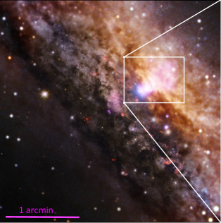
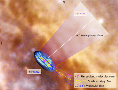
Figure 1: Left: Combined image of X–rays emission from Chandra (low energy: magenta, high energy: blue), overlaid on an optical image from the European Space Observatory. Credits from NASA/CXC/Univ degli Studi Roma Tre/Marinucci et al. (2012), Optical: ESO/VLT & NASA/STScI. Right: Cartoon of the central region ($<$1 kpc) of NGC 4945. The optical image shown in the left panel is used as the background. The size (diameter) of the different components observed in the (soft and hard) X–ray, near-IR and radio bands are highlighted: the limb-brightening ‘plume’ in soft X–ray as well as the nuclear hard X–ray emission region (Marinucci et al. 2012), the starburst ring in Pa$\alpha$ (Marconi et al. 2000) and the nuclear molecular disk along with the unresolved molecular core (Henkel et al. 2018).

1 Introduction

Galaxy interactions and mergers play important roles in the formation and evolution of galaxies, able to trigger massive starburst (SB) and also feed super massive black hole (SMBH). The study of the active galactic nuclei (AGN) and starburst phenomena is a key point in order to understand the relationship between the star formation and AGN activity in galaxies.

The presence of powerful outflows are believed to play an important role in the evolution of galaxies, able to regulate both the star formation and the growth of the SMBH through ‘positive’ or ‘negative’ feedback in young galaxies (e.g., Hopkins et al. 2009; Cresci et al. 2015). Recently the evidence of massive molecular outflows in AGN and SB galaxies strongly support the study of outflowing molecular gas as a process able to quickly remove from the galaxy the gas that would otherwise be available for star formation (‘negative feedback’ on star formation; Sakamoto et al. 2009; Alatalo et al. 2011; Chung et al. 2011; Sturm et al. 2011; Spoon et al. 2013; Cicone et al. 2014; García-Burillo et al. 2014).

The molecular gas plays not only a key role as fuel in the activity process but should also, in turn, be strongly affected by the activity. Depending on the evolutionary phase of the activity, different physical processes can be involved, changing the excitation conditions and the chemistry: strong ultraviolet (UV) radiation coming from young massive stars (i.e., photon dominated region or PDR; e.g., Wolfire et al. 2010), highly energetic X–ray photons coming from an AGN (i.e., X–ray dominated region or XDR; Meijerink et al. 2006), as well as shocks and outflows/inflows (see Flower et al. 2010). X–rays can penetrate more deeply into the ISM than UV photons (Maloney et al. 1996; Maloney 1999; Meijerink & Spaans 2005): X–rays are able to heat more efficiently the gas, but not the dust, and they are less effective in dissociating molecules (Meijerink et al. 2013). On the other hand, PDRs are more efficient than XDRs in heating the dust. For this reason, AGNs are suspected to create excitation and chemical conditions for the surrounding molecular gas that are spatially quite different from those in SB environments. The knowledge of the composition and properties of the molecular gas in such environments is essential to characterize the activity itself, and to differentiate between AGN and SB mechanisms.

We focus our analysis on the nearby (D$\sim$3.8 Mpc; Karachentsev et al. 2007), almost edge-on ($i$ = 78^∘) galaxy, NGC 4945, known to be a remarkable prototype of AGN-SB composite galaxy. Its proximity (1″$\sim$19 pc) makes this object an excellent target for studies of molecular gas at the center of an active galaxy. It is also one of the closest galaxies in the local universe that hosts both an AGN and a starburst. The black hole mass estimated from the velocity dispersion of 150 km s^-1 obtained from the water maser is around $\sim$10⁶ M_⊙ similar to that of our own Galaxy and a factor of 10 smaller than the black hole hosted in the Sy2 galaxy NGC 1068 (1.5 $\times$ 10⁷ M$\odot$; Greenhill & Gwinn 1997). Together with Circinus, it contains a highly obscured Seyfert 2 nucleus (Iwasawa et al. 1993; Marinucci et al. 2012; Puccetti et al. 2014) with associated dense molecular clouds, bright infrared emission, compact (arcsec) radio source, bright H₂O ‘megamaser’ ($\sim$15 mas; Greenhill et al. 1997), strong Fe 6.4 KeV line and variable X–ray emission (Schurch et al. 2002). These observations have revealed a Compton–thick spectrum with an absorbing column density of N_H$\sim$2.4–4$\times$10²⁴ cm^-2 (Guainazzi et al. 2000; Itoh et al. 2008). The nucleus of NGC 4945 is one of the brightest extragalactic sources at 100 keV (Done et al. 1996), and the brightest Seyfert 2 AGN at $>$ 20 keV (Itoh et al. 2008), whose emission is only visible through its reflected emission below 10 keV, due to the large column density that completely absorbs the primary nuclear emission. The emission at higher energy is still visible, though heavily affected by Compton scattering and photoelectric absorption. The nuclear emission between 2-10 keV is enclosed in a region of 12″$\times$6″, consistent with the starburst ring observed using molecular gas tracers (e.g., Moorwood et al. 1996; Marconi et al. 2000; Curran et al. 2001; Schurch et al. 2002).

From IRAS observations we know that about 75% of the total infrared luminosity of the galaxy (L_IR =2.4$\times$10¹⁰ L_⊙) is generated within an elongated region of $<$12″$\times$9″centered on the nucleus (Brock et al. 1988). This structure, as shown in high-resolution HST-NICMOS observations of the Pa$\alpha$ line, is consistent with a nearly edge-on starburst ring of $\sim$5″-10″ (100-200 pc; radius $\sim$2.5″-5″, Marconi et al. 2000).

Recently, the very inner regions of NGC 4945 have been studied in radio by Henkel et al. (2018), who found a complex structure, composed by a nuclear disk of 10″$\times$2″ enclosing a spatially unresolved molecular core of $\lesssim$2″, consistent with the X–ray source size observed with Chandra (Marinucci et al. 2012). Furthermore, using high density gas tracers (e.g., HCN, CS), they also observed two bending spiral-like arms connected by a thick bar-like structure, extending in the east-west direction from galactocentric radii of $\sim$100 pc out to 300 pc.

A conically shaped wind-blown cavity has been observed to the north-west at different wavelengths, extending out of the galaxy plane from the nucleus, probably produced by a starburst driven wind (Moorwood et al. 1996). In particular, it has been detected at soft X–ray (i.e., the ‘plume’), optical and IR wavelengths (Nakai 1989; Moorwood et al. 1996; Schurch et al. 2002; Mingozzi et al. 2019). The extension of the outflow ranges from $\gtrsim$ 2″ in the X–ray band from Chandra (Marinucci et al. 2012) reaching $\sim$30″ in the optical band, observed with MUSE/VLT (Venturi et al. 2017), and in the X–ray band (Schurch et al. 2002).

In Fig. 1 (left panel) we show a composite view of this galaxy using optical and X–ray emissions from Marinucci et al. (2012). In the right panel we also present a sketch of the observed structures in the inner regions of NGC 4945 at different wavelengths.

In this work we study the molecular composition, as well as the excitation temperature and column density, of the interstellar medium (ISM) in the nucleus of NGC 4945. We apply a local thermodynamic equilibrium (LTE) multi–transition analysis to a dataset of several molecules observed using the Heterodyne Instrument for the Far Infrared (HIFI) onboard Herschel satellite and the single dish Atacama Pathfinder EXperiment (APEX; diameter D = 12 m; Güsten et al. 2006) antenna. The LTE analysis was also applied to 2D imaging spectroscopy of ¹²CO data obtained with the Photoconductor Array Camera and Spectrometer (PACS) and the Spectral and Photometric Imaging REceiver (SPIRE). We focus on the LTE analysis applied using the whole sub-mm and far-IR range for studying ¹²CO, which allows us to characterize the distribution of the heating at different spatial scale: from large (35″,$\sim$700 pc) down to small scales (9.4″,$\sim$200 pc). The aim of this work is to characterize the thermal and density structures at different spatial scales in NGC 4945. Furthermore, the determination of the dominant heating mechanism and the origin of the observed heating pattern in the inner regions of this object are also analyzed. The photometric data allow us to derive the mass of dust and the corresponding mass of gas (once assumed a specific gas-to-dust ratio) and compare with the expectations from the heating mechanisms inferred from the ¹²CO analysis.

The paper is organized as follows: In Section 2 we introduce the observations and the data analysis applied for each instrument. In Section 3 we present the Spectral Energy Distribution (SED) results derived from analyzing photometric data obtained from different instruments, from the far-IR to sub-mm wavelengths. Section 4 is dedicated to the derivation of the column densities and the excitation temperatures obtained using the high spectral resolution HIFI and APEX data for all molecules (¹²CO, ¹³CO, HCN, HNC, HCO⁺, CS, [CI], CH) for spatial scales between 20″-30″($\sim$400-700 pc). In Section 5 we focus our analysis on the thermal and column density structures of ¹²CO using 2D imaging spectroscopy: from SPIRE ($\gtrsim$700 pc) down to smaller spatial scales using PACS ($\lesssim$200 pc). Section 6 is devoted to the discussion of the results in order to understand the origin of both gas and dust heating mechanisms. Our main conclusions are summarized in Section 7. Appendix A presents detailed information on the derivation of the flux densities used in the SED fitting analysis (§ 3). Throughout the paper we consider H₀ = 71 km s^-1 Mpc^-1, $\Omega_{M}$ = 0.27 and $\Omega_{\Lambda}$=0.73.

2 Observations and data analysis

2.1 Observations

Table 1: General properties of the HIFI, PACS and SPIRE ¹²CO observations.

Instrument	Type Obs	12CO trans (J+1$\rightarrow$J) or band ($\mu$m)	Obs ID (1342)	Level data	PI
(1)	(2)	(3)	(4)	(5)	(6)
HIFI	Spectroscopic	5$\rightarrow$4 to 9$\rightarrow$8	200939, 200989, 200944	2.5	R. Güsten
PACS	Spectroscopic	15$\rightarrow$14; 20$\rightarrow$19	247789	2	C. Hailey
PACS	Photometric	70; 100; 160	223660; 203022	2.5	E. Sturm
SPIRE	Spectroscopic	4$\rightarrow$3 to 8$\rightarrow$7; 9$\rightarrow$8 to 13$\rightarrow$12	212343	2	E. Sturm
SPIRE	Photometric	250; 350; 500	203079	2	E. Sturm

Notes: Column (1): Instrument; Column (2): type of observation; Column (3): ¹²CO transitions or band; Column (4): ID of the observation. The code ‘1342’ has to be added before the number; Column (5): level of the data used (see text for details); Column (6): principal investigator of the observation.

2.1.1 Heterodyne Instrument for the Far Infrared (HIFI) and the Atacama Pathfinder EXperiment (APEX)

The HIFI observations are taken in the pointed dual beam switch (DBS) mode covering the frequency range between 480 GHz to 1270 GHz (band 1 to 5; see Jackson & Rueda 2005) and from 1410 GHz up to 1910 GHz (bands 6 and 7; see Cherednichenko et al. 2002) at high spectral resolution (R = 10⁶-10⁷). The half-power beam width (HPBW) of the telescope was 37″ and 12″ at 572 GHz and 1892 GHz, respectively. The HIFI Wide Band Spectrometer (WBS) was used with an instantaneous frequency coverage of 4 GHz and an effective spectral resolution of 1.1 MHz. Two orthogonal polarizations (horizontal, H, and vertical, V) were recorded and then combined together to end up with a higher signal-to-noise ratio (SNR). We used the standard Herschel pipeline Level 2.5 which provides fully calibrated spectra (de Graauw et al. 2010; see Tab. 1). In particular, the HIFI Level 2.5 pipeline combines the Level 2 products into final products. Single-point data products are stitched spectra for each of the polarizations and backends applicable to the observation. The spectra were produced using the pipeline version Standard Product Generation (SPG) v14.1.0 within HIPE. For further information see Shipman et al. (2017).

In addiction to the HIFI data we obtained sub-mm data of lower transitions (J_up = 3, 4) of ¹²CO, ¹³CO, HCN, HNC and HCO⁺ using the FLASH+ receiver at 345 GHz at APEX (see Tab. 2). The half-power beam width (HPWB) ranges between 21″ down to 17″ at 272 and 354 GHz, respectively. The spectral resolution provided by a Fourier Transform Spectrometer (FTS) was smoothed to a velocity resolution of 20 MHz. The data reduction was initially performed using CLASS and then imported in MADCUBA (Rivilla et al. 2016; Martín et al. 2019).

2.1.2 Photoconductor Array Camera and Spectrometer (PACS)

PACS is a photometer and a medium resolution spectrometer. In Imaging dual-band photometry, PACS simultaneously images the wavelength range between 60-90 $\mu$m, 90-130 $\mu$m and 130-210 $\mu$m over a field of view (FoV) of 1.75^′ $\times$ 3.5^′. PACS’ grating imagining spectrometer covers the 55-210 $\mu$m spectral range with a spectral resolution between 75-300 km s^-1 over a FoV of 47″$\times$47″, resolved into a 5$\times$5 spaxels, each of them with an aperture of 9.4″.

PACS data were provided from the Herschel archive using Level 2 and 2.5 products (see Tab. 1). The PACS Level-2 spectroscopy products can be used for scientific analysis. Processing to this level contains actual spectra and is highly observing modes dependent. The result is an Image of Cube products (for further details see Poglitsch et al. 2010). The Level-2.5 photometric products are maps (produced with JScanam, Unimap and the high-pass filter pipelines) generated by combining scan and cross-scan observations taken on the same sky field. The PACS products were produced using the pipeline version SPGv14.2.2 within HIPE.

Table 2: Line transitions and instrument used.

Line (Transition)	Rest frequency $\nu$	Instrument
	(GHz)
(1)	(2)	(3)
12CO J= 3 $\rightarrow$ 2	345.79	APEX
12CO J= 5 $\rightarrow$ 4	576.27	HIFI
12CO J = 6 $\rightarrow$ 5	691.47	HIFI
12CO J = 9 $\rightarrow$ 8	1036.91	HIFI
13CO J= 3 $\rightarrow$ 2	330.59	APEX
13CO J = 6 $\rightarrow$ 5	661.07	HIFI
13CO J = 9 $\rightarrow$ 8	991.33	HIFI
HCN J = 4 $\rightarrow$ 3	354.50	APEX
HCN J = 6 $\rightarrow$ 5	531.72	HIFI
HCN J = 7 $\rightarrow$ 6	620.30	HIFI
HCN J = 12 $\rightarrow$ 11	1062.98	HIFI
HNC J= 3 $\rightarrow$ 2	271.98	APEX
HNC J = 4 $\rightarrow$ 3	362.63	APEX
HNC J = 6 $\rightarrow$ 5	543.89	HIFI
HNC J = 7 $\rightarrow$ 6	634.51	HIFI
HCO+ J = 4 $\rightarrow$ 3	356.73	APEX
HCO+ J = 6 $\rightarrow$ 5	356.73	HIFI
HCO+ J = 7 $\rightarrow$ 6	356.73	HIFI
CS J = 6 $\rightarrow$ 5	293.91	HIFI
CS J = 7 $\rightarrow$ 6	342.88	HIFI
CS J = 10 $\rightarrow$ 9	489.75	HIFI
CS J = 12 $\rightarrow$ 11	538.69	HIFI
CS J = 13 $\rightarrow$ 12	587.62	HIFI
[CI] 3P1 $\rightarrow$ 3P0	492.16	HIFI
CH ${}^{2}\Pi_{1/2}$ J = 3/2–1/2	532.72	HIFI
CH ${}^{2}\Pi_{1/2}$ J = 3/2–1/2	536.76	HIFI
CH ${}^{2}\Pi_{3/2}$ J = 5/2–3/2	1656.97	HIFI

Notes: Column (1): line and rotational transition (J); Column (2): frequency of the molecule in giga hertz (GHz); Column (3): instrument used for the observation.

Table 3: SPIRE beams in the photometric and spectroscopic modes.

Subinstrument		Photom		SPectr
	PSW	PMW	PLW	SSW	SLW
band ($\mu$m)	250	350	500	192-313	303-671
beam (FWHM)	17.6″	23.9″	35.2″	17″-21″	29″-42″

2.1.3 Spectral and Photometric Imaging REceiver (SPIRE)

SPIRE consists of a three band imaging photometer and an imaging Fourier Transform Spectrometer (FTS). The photometer carries out broad–band photometry ($\lambda$/$\Delta\lambda$$\approx$3) in three spectral bands centered on approximately 250, 350 and 500 $\mu$m with an angular resolution of about 18″, 24″and 35″, respectively (see Tab. 3). The spectroscopy is carried out by a FTS that uses two overlapping bands to cover 194-671 $\mu$m (447-1550 GHz) simultaneously, the SSW short wavelength band (190-313 $\mu$m; 957-1577 GHz) and SLW long wavelength band (303-650 $\mu$m; 461-989 GHz). The SPIRE–FTS is a low spatial and spectral (1.2 GHz) resolution mapping spectrometer. In particular, the beam full width at half–maximum (FWHM) of the SSW bolometers is 18″, approximately constant with frequency. The beam FWHM of the SLW bolometers varies between $\sim$30″ and 42″ with a complicated dependence on frequency (Swinyard et al. 2010).

We use SPIRE Level-2 spectroscopic and photometric products for our analysis. These data are processed to such a level that scientific analysis can be performed. The SPIRE Level-2 photometer products (maps) are calibrated in terms of in-beam flux density (Jy/beam). The photometric and spectroscopic SPIRE data Level-2 were produced using the pipeline version SPGv14.1.0 within HIPE.

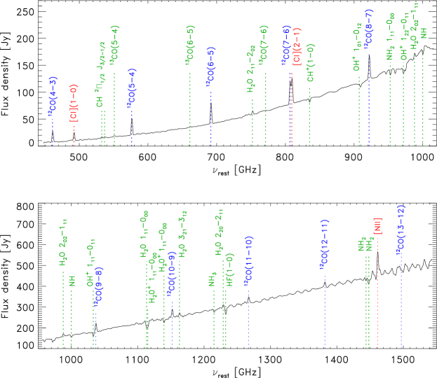
Figure 2: SLW (upper panel) and SSW SPIRE (lower panel) spectra corresponding to the peak emission in the same FoV in the rest-frame frequency. ¹²CO lines are shown in blue while fine structure lines, as [CI] and [NII], are indicated in red. Other molecular species observed in emission and/or in absorption are shown in green.

Our data have been achieved with an intermediate spatial sampling: in such a case, the pixel size for the SLW and SSW bolometers are 35″ and 19″, respectively. The ¹²CO ladder (from J_up = 4 to 13) is the most prominent spectral feature in this frequency range. These mid-J ¹²CO emission lines probe warm molecular gas (upper-level energies ranging from 55 K to 500 K above the ground state) that can be heated by ultraviolet photons, shocks, or X–rays originated in the active galactic nucleus or in young star-forming regions. In the SPIRE–FTS range besides the ¹²CO transitions we also detected the prominent [CI]492 $\mu$m, [CI]809 $\mu$m and [NII]205 $\mu$m transitions across the entire system along with several molecular species observed in absorption (see Fig. 2). A baseline (continuum) subtraction of second or third order has been applied to these spectra. Detailed information on the SPIRE observations are summarized in Tab. 1.

2.2 Data analysis

Using high spectral resolution HIFI and APEX data we carried out multi-line analysis of ¹²CO, ¹³CO, HCN, HCN, HCO⁺, CS, [CI], CH which have been all detected in emission. Other molecules such as NH, NH₂, OH⁺, HF, H₂O have been detected in absorption and they will be analyzed in feature work. HIFI and APEX products are calibrated in antenna temperature (T${}^{\star}_{A}$). This was converted to main beam temperature (T_MB) according to the relation:

$$\hskip 28.45274ptT_{MB}=\frac{\eta_{f}}{\eta_{MB}}\hskip 8.53581ptT^{\star}_{A},$$ (1)

where $\eta_{f}$ is the forward efficiency of the telescope and $\eta_{MB}$ is the main beam efficiency. For the HIFI data $\eta_{MB}$ ranges from 0.69 to 0.76 with a $\eta_{f}$ = 0.96, while for the APEX data we used a $\eta_{MB}$ = 0.73 and $\eta_{f}$ = 0.97. The main beam temperature T_MB has been corrected for beam dilution, according to the relation:

$$\hskip 28.45274ptT^{\prime}_{MB}=\left(\frac{\theta^{2}_{s}+\theta^{2}_{b}}{\theta^{2}_{s}}\right)\hskip 5.69054ptT_{MB},$$ (2)

where $\theta_{s}$ and $\theta_{b}$ are the source size and the beam size, respectively. For this object a source size of 20″ has been considered (Wang et al. 2004).

The HIFI spectra were smoothed to a resolution of 20 km s^-1. When needed, further smoothing and baseline corrections have been applied to the spectra to improve the signal-to-noise ratio (SNR).

The molecular emission was modeled with SLIM package within MADCUBA (Martín et al. 2019). In the model, SLIM fits the synthetic LTE line profiles to the observed spectra. The fit is performed in the parameter space of molecular column density N_mol, excitation temperature T_ex, velocity v_LSR and width of the line (FWHM) to the line profile and source size. SLIM allows the presence of different components (‘multi Gaussian fit’), which can be differentiated using different physical parameters (e.g., column density, excitation temperature, velocity). In case of multiple transitions fit, two (or more) T_ex can be also assumed (‘multiple excitation temperature’, see § 3.3.2 in Martín et al. 2019).

To properly account for the beam dilution factor, a source size was fixed as an input parameter.

3 Continuum analysis

3.1 Intrinsic source size of the dust emission from PACS and SPIRE photometry

Table 4: Intrinsic source size using PACS and SPIRE photometric data.

Band–	Nominal	Intrinsic	Flux	PSF
Instrument	pixel size	source size	density
($\mu$m–)	(″)	(″$\times$ ″)	(Jy)	(″)
(1)	(2)	(3)	(4)	(5)
70 PACS	1.6	7.4$\times$3.5 (0.5)	258 (5)	5.5
100 PACS	1.6	8.1$\times$3.7 (0.8)	340 (9)	7.2
160 PACS	3.2	9.3$\times$2.8 (1.6)	329 (19)	11.5
250 SPIRE	6	13.9$\times$5.8 (2.0)	235 (6)	17.6
350 SPIRE	10	21.7$\times$3.8 (3.3)	$<$95(a)	23.9
500 SPIRE	14	16.3$\times$$<$35 (4.7)	34 (0.3)	35.2

Notes: Column (1): Photometric band and instrument; Column (2): nominal pixel size of the instrument for the specific band; Column (3): intrinsic source size (and uncertainty) obtained deconvolving the observed source size for the corresponding point spread function (PSF) value; Column (4): flux density enclosed in the observed source size; Column (5): PSF in the different bands. ^(a) Lower limit value due to the presence of a bad pixel enclosed in the observed source size.

In this section we derived the intrinsic (deconvolved) size of the different components of the dust emission in NGC 4945, as small and large grains along with polyaromatic hydrocarbons (PAH’s; Lisenfeld et al. 2002; da Cunha et al. 2008), using the photometric data from PACS (70, 100, 160 $\mu$m) and SPIRE (250, 350, 500 $\mu$m). These photometric images have been retrieved from the Herschel archive (see Tab. 1). We measured the FWHM sizes of the peak emission and we deconvolved them with the relevant PSF sizes assuming gaussian shapes for both. At these moderate resolutions the galaxy shows the presence of a compact source plus a disk component: at these wavelengths the contribution of the compact source emission dominates over the disk component within the beam. The results of the intrinsic source size are listed in Tab. 4.

We then computed the flux density enclosed in the observed source size. For the PACS data the maps are in units of [Jy pixel^-1] while the SPIRE maps (point source calibrated) are in units of [Jy beam^-1]. Thus, to compute the total flux density included in the (observed) source size, we treated the two dataset as follows: for the PACS data we simply sum all fluxes of each pixel within the estimated source size while for the SPIRE data we multiply the sum of all values within the source size by a factor of $(pixel$ $size/PSF)^{2}$ at the corresponding wavelength (Tab. 4). From these results the emission of NGC 4945 is resolved in both directions at all but one PACS and SPIRE wavelengths: in particular, at 500 $\mu$m the emission is resolved in one direction and unresolved in the perpendicular direction. The photometric PACS and SPIRE maps are shown in Fig. 3.

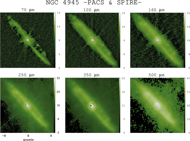
Figure 3: Photometric images of NGC 4945 at the PACS (70, 100 and 160 $\mu$m; top) and SPIRE (250, 350 and 500 $\mu$m; bottom) wavelengths. The flux units have been converted to Jansky for both the PACS and SPIRE data (see text for details). The black circle in each panel identifies a beam of 40″$\times$40″. From PACS 70 $\mu$m to SPIRE 500 $\mu$m wavelengths an aperture of 40″ corresponds to 25, 25, 12.5, 6.7, 4 and 3 pixels, respectively. The black cross represents the peak emission in each band.

3.2 Spectral Energy Distribution of NCG 4945

We derived the spectral energy distribution (SED) combining PACS and SPIRE data with those obtained at sub-mm wavelengths from Weiß et al. (2008) using Large APEX Bolometer Camera (LABOCA) and from Chou et al. (2007) using the the Submillimeter Array (SMA) within an aperture of 40″$\times$40″ (see Fig. 4). This is a reasonable value to consider most of the emission from the inner regions of the galaxy at all wavelengths: the aperture considered is shown in Fig. 3 for both PACS and SPIRE bands. The flux density obtained in Weiß et al. (2008) in an aperture of 80″$\times$ 80″ has been scaled to our aperture, deriving a flux density of 9.05 ($\pm$ 1.3) Jy (see App. A for details). We also added one far-IR data point from MSX at $\sim$20 $\mu$m. Other data at shorter wavelengths were available from MSX, IRAC and 2MASS catalogues but they were not included in this analysis because their emission (in the range $\sim$3-17 $\mu$m) is strongly affected by several emission features from PAH molecules (see Povich et al. 2007; Pérez-Beaupuits et al. 2018). In Tab. 5 the derived flux densities are shown.

Table 5: Continuum flux density values in the far-IR and sub-mm wavelengths range.

Data	Wavelength	Frequency	Flux	Flux density
			density	MBB
	($\mu$m)	(GHz)	(Jy)	(Jy)
(1)	(2)	(3)	(4)	(5)
MSX	21.34	14058	6 (2)	7
PACS	70	4286	694 (138)	620
PACS	100	3000	988 (198)	1020
PACS	160	1875	753 (151)	845
SPIRE	250	1200	430 (86)	370
SPIRE	350	857	142 (28)	150
SPIRE	500	600	44 (9)	45
LABOCA	870	345	9.1 (1.3)	7
SMA	1300	230	1.0 (0.3)	1.4

Notes: Column (1): Instrument; Column (2): central wavelength in $\mu$m; Column (3): values of Column (2) in frequency, given in GHz; Column (4): flux densities (and uncertainty) in Jansky computed in an aperture of 40″$\times$40″. For the SPIRE and PACS data we consider uncertainties of 20% of the flux density. Column (5): flux density values of the total modified black body (MBB) modeled emission (red solid line in Fig. 4).

From the SED fitting we are able to constrain the source size, $\Omega_{s}$, the dust temperature, T_d, and the total mass of dust, M_dust (as done in Weiß et al. 2008). To properly fit the dust emission an attenuated black body function (i.e., modified black body) is considered. The source function, S_ν, of the dust is related to the Planck’s blackbody function (B_ν) at the dust temperature (T_d), the dust opacity ($\tau_{\nu}$) and the source solid angle ($\Omega_{s}$) according to the formula:

$$\hskip 8.53581ptS_{\nu}=B_{\nu}(\nu,T_{d})\times(1-e^{-\tau(\nu)})\times\Omega_{s},$$ (3)

while the dust optical depth was computed as

$$\hskip 8.53581pt\tau_{\nu}\leavevmode\nobreak\ =\leavevmode\nobreak\ \kappa_{d}(\nu)\times\frac{M_{dust}}{D^{2}\Omega_{s}}.$$ (4)

D is the distance to the source and $\kappa_{d}(\nu)$ is the dust absorption coefficient, in units of m² kg^-1 (Krugel & Siebenmorgen 1994). $\kappa_{d}$($\nu$) is related to the $\beta$ parameter according to the relation: $\kappa_{d}$($\nu$) = 0.04 $\times$ ($\nu$/250 GHz)^β. In this work $\beta$ has been computed using SPIRE, LABOCA and SMA data, obtaining a value of 2.0 from the linear fit. A source size of 20″$\times$10″ has been assumed.

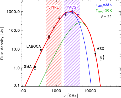
Figure 4: SED fitting results for NGC 4945. The best fit solution (red solid line) is obtained when two dust components with a temperature of 28 K (blue MBB) and 50 K (green MBB) are needed, assuming source size of 20″$\times$10″. The total dust mass obtained from the fit is $\lesssim$10⁷ M_⊙. The SPIRE and PACS data are shown using red and violet squares, respectively. Additional data used in the fit are shown in filled black squares. In particular, at shorter frequencies the SMA (Chou et al. 2007) and LABOCA (Weiß et al. 2008) data were added (see text for details) obtaining a $\beta$ parameter of 2.0. At higher frequencies the MSX data point is considered in the fit while two IRAC data points are only shown for completeness (in gray).

In Fig. 4 the best fit SED ($\chi^{2}_{min}$$\sim$ 4.6; red solid line) is derived when two component temperatures dust model are considered: a cold dust component at 28 K to fit the shorter frequencies and a warm component at 50 K to fit the higher frequencies. A total mass of dust of $\sim$8 $\times$10⁶ M_⊙ is derived. Assuming a gas-to-dust ratio in between 100 and 150 (see Weiß et al. 2008), we derived a total gas mass of 7.6-11.4$\times$10⁸ M_⊙.

We found a good agreement with the results obtained from previous works. Indeed, Weiß et al. (2008) derived a total mass of gas in the central region using an aperture of 80″$\times$80″ of 1.6$\times$10⁹ M_⊙. Comparing their results with the one we derived we can conclude that most of the total emission (70%) is included in a region of 40″$\times$40″.

On the other hand, Chou et al. (2007) estimated the mass of molecular gas from the inferred dust emission at 1.3 mm (i.e, 1 Jy; see Fig. 4), assuming a gas-to-dust ratio of 100. They assumed a dust temperature T_dust$\sim$40 K as inferred from far-infrared measurements (Brock et al. 1988) then deriving, according to their Eq. 1, M_gas$\approx$3.6 $\times$ 10⁸ M_⊙, which corresponds to a mass of dust in the range $\sim$2.4-3.6 $\times$10⁶ M_⊙. The mass of dust derived by Chou et al. (2007) is a factor of 2–3 lower than that derived in our work, and it can be considered as lower limit.

The results of our SED modeling are summarized in Tab. 6.

Table 6: Results obtained from the SED fitting and from the literature.

	Tdust	Mdust	Mgas	GDR	Notes
	(K)	(106 M⊙)	(108 M⊙)
	(1)	(2)	(3)	(4)
This work	28$\pm$1, 50$\pm$2	7.6$\pm$0.3	11.4$\pm$0.5	150
Chou 2007	40	2.4 - 3.6	3.6$\pm$0.7	100	a
Chou 2007	30	3.1 - 4.7	4.7$\pm$0.9	100	a
Wei$\beta$ 2008	20	8 - 12	15.8$\pm$1.6	150	b

Notes: Column (1): temperature of the dust component in kelvin; Column (2): mass of dust in units of 10⁶ M_⊙. In italic font are shown the two M_dust values derived applying a gas-to-dust ratio of 100 and 150, respectively, to the M_gas values taken from literature. Column (3): mass of gas in units of 10⁸ M_⊙. Column (4): gas-to-dust ratio considered; Column (5): notes with the following code: (a) the gas mass has been derived using the dust emission at 1.3 mm according to the Hildebrand (1983) formula (assuming a gas-to-dust ratio of 100); (b) the gas mass of the central region has been derived considering the cold (20 K) and warm (40 K) contributions in an aperture of 80″$\times$80″.

4 Density and temperature determination. Resolved spectra from HIFI and APEX

Table 7: Line parameter results derived using MADCUBA.

Line	$v_{LSR}$	$\Delta v_{1/2}$	T${}^{peak}_{MB}$	Area	Notes
	(km s-1)	(km s-1)	(K)	(K km s-1)
(1)	(2)	(3)	(4)	(5)	(6)
CO(3–2)	451; 566; 706	90; 109 (20); 90	3.05; 3.58; 2.28	294; 456 (75); 220	a
CO(5–4)			0.19; 0.26; 0.13	18; 33 (6); 13	a
CO(6–5)			0.052; 0.08; 0.035	5; 10 (3); 3	a
CO(9–8)			–	–	a, d
CO(3–2)	455; 578; 683	90; 119 (16); 90	0.64; 0.32; 0.64	57.4; 34.4 (5); 57.4	b
CO(5–4)			0.35; 0.18; 0.35	33.4; 21.1 (3); 33.4	b
CO(6–5)			0.44; 0.24; 0.44	42.4; 27.7 (4); 42.3	b
CO(9–8)			0.344; 0.21; 0.34	33.0; 24.4 (4); 32.6	b
13CO(3–2)	446; 566; 685	90; 148 (21); 90	0.36; 0.31; 0.30	35; 48 (9); 29
13CO(6–5)			0.028; 0.015; 0.020	2.7; 2.4 (0.40); 1.9
13CO(9–8)			$<$ 0.06	$<$ 8	c
HCN(4–3)	446; 574; 683	90; 169 (19); 90	0.12; 0.095 ; 0.13	11.33; 17.04 (3); 12.39
HCN(6–5)			0.008; 0.004 ; 0.008	0.90; 0.84 (0.3); 0.90
HCN(7–6)			0.0035; 0.0012; 0.0035	0.34; 0.22; 0.34
HCN(12–11)			$<$0.1	$<$ 1	c
HNC(3–2)	448; 572; 683	90; 138 (18); 90	0.064; 0.043; 0.063	6.2; 6.4 (0.9); 6.0
HNC(4–3)			0.056; 0.04; 0.059	5.4; 5.9 (0.96); 5.7
HNC(6–5)			0.002; 0.002; 0.002	0.22; 0.34 (0.09); 0.22
HNC(7–6)			$<$ 0.06	$<$ 6	c
HCO+(4–3)	450; 580; 685	90; 176; 90	0.13; 0.11; 0.14	12.2; 21.3; 12.4
HCO+(6–5)			0.004; 0.004; 0.004	034; 0.66; 0.34
HCO+(7–6)			$<$ 0.02	$<$ 2	c
CS(6–5)	444; 564; 671	90; 129 (28); 90	0.023; 0.029; 0.027	2.24; 3.92 (1.07); 2.61
CS(7–6)			0.021; 0.028; 0.027	2.03; 3.82 (0.97); 2.54
CS(10–9)			$<$ 0.02	$<$ 2	c
CS(12–11)			$<$ 0.02	$<$ 3	c
CS(13–12)			$<$ 0.03	$<$ 4	c
[CI] 3P1 $\rightarrow$ 3P0	448; 568; 688	90; 152 (23); 90	0.24; 0.24; 0.20	23; 39 (8); 20
$[$CI$]$ 3P2 $\rightarrow$ 3P1			0.33; 0.32; 0.38	33; 52 (10); 37
CH(3/2–1/2)	438; 556; 698	90; 150 (18); 90	0.041; 0.023; 0.037	4.59; 4.29; 4.14
CH(3/2–1/2)			0.041; 0.024; 0.037	4.59; 3.13; 4.14
CH(5/2–3/2)			$<$ 0.06	$<$ 5	c

Notes: Column (1): Molecule and rotational transition (J); Column (2): centroid of the gaussian component (local standard of rest velocity, v_LSR) in km s^-1; Column (3): full width at half maximum (FWHM) of the gaussian in km s^-1. The error values have been computed only for the central component for which the FWHM has been let free to vary. For the blue and red components the FWHM has been fixed to 90 km s^-1; Column (4): main beam peak temperature of each gaussian in kelvin; Column (5): area of the gaussian component in K km s^-1; Column (6): notes with the following code: (a) cold component; (b) hot component; (c) 3$\sigma$ upper limit; (d) the cold component does not exist for this transition.

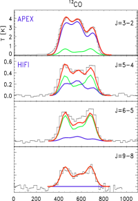
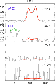
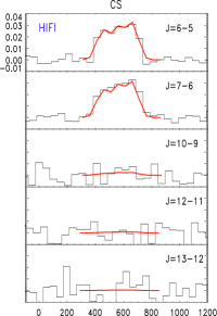
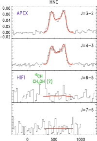
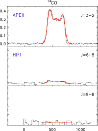
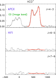
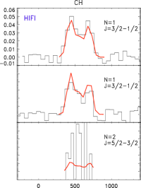
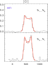
Figure 5: High resolution molecular spectra from APEX and HIFI for all molecules analyzed in this work. In black the observed spectra, in red the LTE fit obtained using MADCUBA. Only for the ¹²CO molecule we highlight a cold (blue) and a hot (green) components because two temperature components were needed to properly fit the emission. For each APEX (J${}_{up}<$ 4) and HIFI (J${}_{up}>$ 5–9) spectra the J transitions are identified. In green other molecular species like CH, ¹³CH and ¹²CO (in the image band) are detected. For each molecule the range in temperature is the same for all J (APEX and HIFI) transitions with the exception of the ¹²CO and HCN which show different ranges to better appreciate the fainter emission of the HIFI data. The emission is shown in main beam temperature (T_MB) in kelvin.

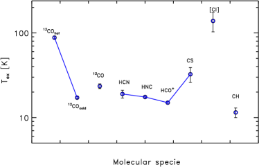
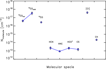
Figure 6: LTE results derived with MADCUBA for each individual molecular specie. From left to right: the excitation temperature, T_ex, in kelvin, along with the molecular column density, N_mol, in units of cm^-2, are shown.

4.1 LTE results using MADCUBA

We apply the LTE analysis using MADCUBA (Martín et al. 2019) to ¹²CO, ¹³CO, HCN, HNC, HCO⁺, CS, [CI], CH molecules observed using the high spectral resolution HIFI and APEX data. A source size of $\theta$=20″ has been assumed (see § 2.2). The observed spectra and the simulated emission from the LTE model are shown in Fig. 5. All molecules except ¹²CO have been properly fitted using one temperature component. Indeed, in the specific case of ¹²CO, the emission has been fitted using two temperature components (top left panel in Fig. 5): the one cold and more dense while the other warm and less dense. The cold component ($\sim$20 K; in blue) dominates the emission characterizing the low J transitions while the warm one ($\sim$90 K; in green) dominates the emission at higher J. The need of two different (LTE) excitation temperatures T_ex to fit all the line profiles is a clear indication of non–LTE excitation due to temperature and/or density gradients. The physical conditions required to explain the molecular excitation will be discussed in the next subsection.

The combination of low rotational transitions (J = 3–2 or 4–3) from APEX with higher rotational transitions from HIFI (J = 5–4 up to 9–8) allows to better constrain the molecular column density N_mol and excitation temperature T_ex parameters for each specie (see § 2.2). The typical value of N_mol derived for ¹²CO with MADCUBA ranges from 4$\times$10¹⁶ cm^-2 up to 3.2$\times$10¹⁷ cm^-2, for the warm and cold components, respectively. The N_mol and T_ex values for the different molecules are shown in Fig. 6.

According to the LTE analysis, we then derived the following results (see Tab. 7) for all molecules:

1. Three distinct kinematic components have been found for all molecules: they identify the nuclear bulk ($\sim$560 km s^-1) and the rotating disk structures which show one blue– ($\sim$450 km s^-1) and one red–shifted ($\sim$690 km s^-1) components. Our result is an agreement with the kinematics derived in previous works (e.g., Ott et al. 2001; Henkel et al. 2018);

2. All the species, except ¹²CO and [CI], have been properly fitted using a single excitation temperature of about 20 K. ¹²CO needs two components with excitation temperatures of 20 K and 90 K while [CI] needs one component with a high excitation temperature, T_ex $\sim$ 150 K;

3. The typical value of N_mol derived for low density gas tracers, such as ¹²CO, ¹³CO, [CI] ranges from 3$\times$10¹⁶ cm^-2 up to 5$\times$10¹⁷ cm^-2. For the low density tracer CH the lowest column density is achieved (N_mol $\sim$ 10¹⁴ cm^-2). The derived N_mol for the high density gas tracers such as HCN, HNC, HCO⁺ and CS, has a lower value, of the order of 10¹³ cm^-2. If a smaller source size was considered (i.e., $\theta_{s}$=10″), as in Henkel et al. 2018, the column density values would have been increased by a factor of $\lesssim$3.

Table 8: Results derived from LTE (MADCUBA) and non–LTE (RADEX) analyses using Herschel/HIFI and APEX data.

Molecule	log Nmol	Tex	n(H2)	log Nmol	Notes
			RADEX
	(cm-2)	(K)	(cm-3)	(cm-2)
(1)	(2)	(3)	(4)	(5)	(6)
12CO	16.6 - 16.8	84-92	5.9$\times$104	16.75	a,b
	17.4 - 17.8	16-18	7.3$\times$103	17.41
13CO	16.39 - 16.59	22-25	3.8$\times$103	16.35	c
HCN	13.28 - 13.58	17-21	1.2$\times$106	13.39	d
HNC	13.03 - 13.05	17-18	1.4$\times$106	13.00	d
HCO+	13.29 - 13.53	15	5.0$\times$105	13.76	d
CS	13.11 - 13.39	26-39	8.0$\times$105	13.15	d
[CI]	17.57 - 17.77	103-174	1.0$\times$105	17.56	e, f
CH	14.32 - 14.50	10-13	—	—	e, g

Notes: Column (1): molecule; Column (2): molecular column density (logarithmic value) in units of cm^-2; Column (3): excitation temperature in kelvin; Column (4): hydrogen volume density obtained using RADEX in units of cm^-3; Column (5): molecular column density derived with RADEX in units of cm^-2; Column (6): notes with the following code: (a) two (i.e., cold and warm) components fit; (b) all transition detected; (c) J=9–8 not detected; (d) HIFI transitions not detected; (e) only HIFI data; (f) extended source ($>$20″); (g) n(H₂) and N_mol cannot be derived since this molecule is not present in the RADEX online code.
The kinetic temperature and the source size considered in the RADEX analysis are, respectively, T${}_{kin}=$ 200 K and $\theta_{s}=$ 20″.

4.2 non–LTE results using the RADEX code

As mentioned above, the need of two different LTE excitation temperatures T_ex to fit all the ¹²CO line profiles (from J_up = 3 up to 9) is a clear indication of a non–LTE excitation of this molecule. We then apply the non–LTE RADEX code to derive the volume gas density of the collisional patter, n(H₂), in NGC 4945 for each molecular specie, and to confirm the molecular column densities, N_mol, and the excitation temperature, T_ex, values derived with MADCUBA LTE analysis, restricted to the rotational J transitions of the specific molecule involved in the analysis (§ 4.1).

The RADEX code is based on a non–LTE analysis taking advantage of the velocity gradient (i.e., N_mol/$\Delta$v, the ratio between the column density, in cm^-2, and line width, in km s^-1). This code was used to predict the line emission from all molecules, using all the lines simultaneously, and considering a kinetic temperature of 200 K. This assumption is based on the T_ex derived for CO and [CI] (i.e., $\sim$150 K; see previous section). In fact, in the case of ¹²CO, we carried out the analysis for two different kinematic temperatures: T_kin = 50 K when fitting the cold component and T_kin = 200 K for the warm component. A lower T_kin would not be able to properly reproduce the line profiles of the ¹²CO transitions at higher frequencies (e.g., J=6-5). For most of the transitions observed in this work, except for ¹²CO involved levels with energies below 50 K, the choice of the T_kin has a marginal effect in the derived H₂ densities and the molecular column densities.

To derive the H₂ densities and the molecular column densities, N_mol, from RADEX we have tried to fit all the observed ¹²CO lines with a isothermal and uniform cloud but we did not find a unique solution. To fit all lines it was required to have at least two clouds with different densities and/or temperatures. These results indicate the presence of molecular clouds with a range of densities and temperatures within the beam, as expected for the complexity of the NGC 4945 nucleus. The predicted non–LTE ¹²CO column densities for the two different H₂ density regimes are similar to those derived from the LTE analysis. The comparison of the predicted non–LTE T_ex with the derived LTE values is more complicated since there is not a single non–LTE T_ex, but a range of T_ex depending on the excitation requirements for each transition. The situation is even more complicated for the case of a non–uniform molecular cloud with H₂ density gradients exciting different ¹²CO lines in different regions. As illustrated by the non–LTE analysis, lower J lines will be more sensitive to low densities than the high–J lines. We have then compared the average of the predicted non–LTE T_ex with the LTE T_ex for the range of transitions that dominates the ¹²CO emission. We have found a reasonable agreement between both temperatures for the low– and the high–J lines corresponding to the low and high density components, respectively.

As expected from the typical density of the ISM in galaxies over the scales of hundreds of pc, most of the high dipole-moment molecules (e.g., HCN, CS, HCO⁺) usually have a critical density much larger than the average H₂ density of the ISM. We then derive subthermally excitation (T_kin$>$T_ex) for all density gas tracers.

According to our results, we derived a moderate volume gas density n(H₂) for most of the molecules, in the range 10³ cm^-3 up to 10⁶ cm^-3. Lower densities are obtained when considering the low density gas tracers (e.g., ¹²CO, [CI]), while higher densities are derived when studying the high density gas tracers, such as HCN, HNC, HCO⁺ and CS (see Tab. 8). We reproduce reasonable well the intensities of all transitions for each molecule with RADEX, also when considering a non-uniform cloud (i.e., two H₂ densities), in agreement with the results derived using MADCUBA, as in the case of the two components model applied to ¹²CO.

5 Thermal and column density structures from the ¹²CO emission at different scales

We study the distribution of the thermal balance and the column density distribution at different spatial scales using the 2D PACS and SPIRE data through the analysis of the ¹²CO emission over a wide range of rotational transitions. In particular, the ¹²CO transitions at wavelengths from 55 $\mu$m to 650 $\mu$m were covered: this molecule is the most abundant in the interstellar medium after H₂ and therefore considered a good tracer of the properties of the bulk of the molecular gas phase. As shown from the analysis of a limited number of ¹²CO transitions (§ 4.1), the wide range of physical properties expected in the nucleus of NGC 4945 cannot be described by either LTE or simple non-LTE modeling. To deal with the full range of ¹²CO transitions and the wide range of spatial scales addressed in this work we will apply a ‘transition limited’ LTE analysis to a given range of transitions sampling specific physical conditions (density and temperatures) of the molecular gas. This analysis will allow us to derive the spatial distribution of ‘transition limited’ T_ex and N_mol, which will describe the different phases of the molecular gas in NGC 4945.

5.1 Mid-J ¹²CO at large spatial scale (700 pc – 2 kpc)

In this section we study the warm component by using the mid– and high–J of ¹²CO rotational transitions from SPIRE long wavelengths (SLW; transitions from J_up = 4 to 8), and from SPIRE short wavelength (SSW; J_up = 9 to 13). For our study we mainly focus on the very central regions of the whole field of view (FoV), where the strongest ¹²CO emission is observed. In particular, a maximum region of 3$\times$3 spaxels at a resolution of 35″($\sim$2$\times$2 kpc²; see left panel in Fig. 7) in the SLW map is considered. For each SLW spectrum we combined the contribution at higher frequencies of 3$\times$3 SSW spectra at a resolution of 19″ ($\sim$1$\times$1 kpc²) to match the beam of the SLW spectrum (middle panel in Fig. 7).

When applying the LTE analysis to all SPIRE data we derived the excitation temperature and column density for each (combined) spectrum at the resolution of 35″ ($\sim$700 pc). From this analysis, we found higher T_ex in the center and in the north part of the galaxy possibly affected by the presence of the outflow at large scales (see § 1). In the remaining regions lower temperatures are found. The column density peaks in the center showing higher values in the south (middle panels in Fig. 8). At this spatial resolution the LTE analysis gives good results when using one temperature component.

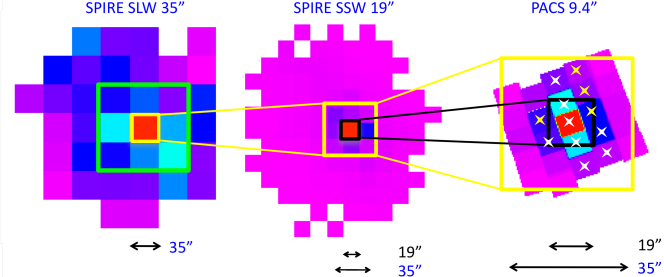
Figure 7: From left to right: Schematic view of the different FoVs involved in the analysis of SLW, SSW SPIRE and PACS data. Left: In the SLW SPIRE map the green square highlights the FoV considered in the analysis ($\sim$100″). These data are characterized by a a beam of 35″ identified by the yellow small square. Middle: in the SSW SPIRE map the yellow square represents the 3$\times$3 spaxels area involved in the analysis. The map is characterized by a beam of 19″ (small black square). Right: in the PACS map the black square identifies a FoV of $\sim$19″ (i.e., one SSW SPIRE spaxel) while the yellow square identifies a FoV of $\sim$35″. The star symbols represent those spaxels where the ¹²CO emission is observed: in particular, white stars highlight the spaxels characterized by stronger ¹²CO emission than that observed in the remaining spaxels marked using yellow stars. PACS data are characterized by a beam of 9.4″.

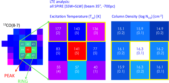
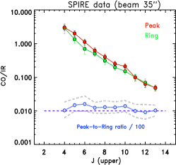
Figure 8: Left: ¹²CO(8–7) emission map showing a FoV of 3$\times$3 spaxels (35″ each; light green square) considered when combining the SSW and SLW SPIRE data at the same resolution (i.e., 35″, large spatial scale). The peak emission (in red) and a ring of one spaxel width around that maximum (green area) are identified. Middle: Excitation temperatures (T_ex) and the (logarithmic) column densities (N_CO) are derived for each spaxel using the rotational diagrams. The yellow boxes represent the spectra characterized by high T_ex and N_CO values. Right: ¹²CO/IR flux ratios computed in correspondence of the flux density peak (red) and the ring (green) for the different transitions J in the SPIRE domain. The ratio between the maximum peak and the ring for each transition is also shown (i.e., ‘peak-to-ring ratio’, in blue) divided by 100 (a factor of 100 has to be applied to obtain the real values). The dashed gray lines identify the lower and upper limit values of the peak-to-ring ratios computed within the errors. Higher ¹²CO/IR values are derived for high J (J${}_{up}\leavevmode\nobreak\ \geq$ 11–10) in the ring structure, implying lower ($\lesssim$ 1) peak-to-ring ratios.

In order to study the spatial distribution of the heating in this galaxy we compare the emission in the peak with the emission integrated in an annular ring around the peak (one spaxel width) using the same beam for all transitions. We computed the ratio between the ¹²CO flux density peak and the corresponding IR continuum emission at each frequency of the ¹²CO as a function of J (hereafter, CO/IR ratios) as shown in Fig. 8 (right panel). For a spectroscopically unresolved line, as in this case, the flux density peak (given in W m^-2 Hz^-1, or Jy) is proportional to its line total flux (W m^-2). We then multiply the IR flux density by the spectral resolution to derive the total integrated IR continuum flux at the wavelength of each line. Since all ¹²CO transitions have similar line widths, the CO/IR ratio corresponds to the flux ratio of each emission line: i.e., Flux(CO)/Flux(IR Continuum). Thus, the ratio is a dimensionless quantity. Instead of using the total infrared flux, like usually considered in the literature (see Meijerink et al. 2013), we consider the continuum underlying each ¹²CO transition to characterize the ¹²CO/IR ratio at the specific continuum value and specific frequency to take into account changes in the shape of the SED.

We found that the CO/IR values derived in the peak position are higher (of a factor of $\lesssim$ 2, within the errors) than those derived in the ring for all rotational transitions up to J_up = 10. This trend changes for J_up $>$ 11 transitions where the emission in the ring becomes higher (or similar) to that of the peak. This result suggests the presence of mechanisms able to increase the emission of ¹²CO at higher frequencies. In what follows we will study in detail this issue using higher resolution data, moving from intermediate to small scales in order to unveiling the origin of this mechanism.

5.2 Mid- and high-J ¹²CO data within the inner 700 pc (large - intermediate scales)

We now combine SPIRE (SSW and SLW) and PACS data at a resolution of 35″ ($\sim$700 pc). These instruments have different PSFs (19″ and 35″ for SPIRE SSW and SLW data, respectively, and 9.4″ for PACS). To properly analyze all the ¹²CO spectra over the whole frequency range we smoothed all data to the the largest PSF (35″). The reference spectrum in the SLW SPIRE data cube is the one corresponding to the ¹²CO peak emission (central spaxel).

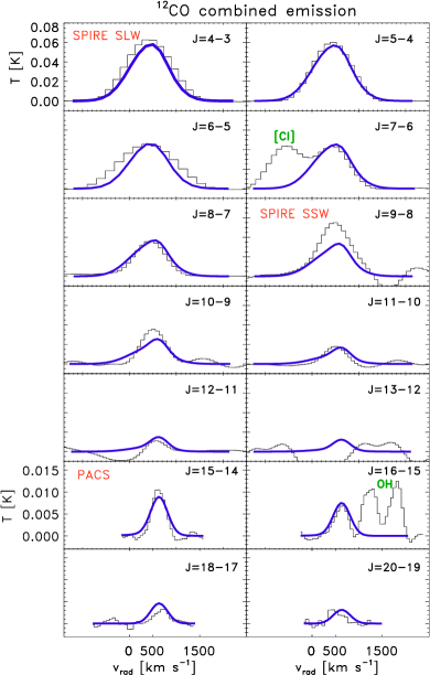
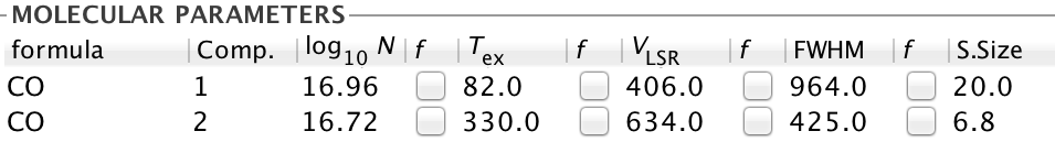
Figure 9: Top: Averaged SLW, SSW SPIRE (J_up = 4 up to 13) and PACS ¹²CO spectra (J_up = 15 up to 20) of the central region combined together at the same resolution (35″). The original spectra are shown in black while the total simulated ¹²CO emission obtained from the LTE approach are shown in blue. In green other molecular species like [CI] and OH are identified in emission. Bottom: Table from MADCUBA showing the output parameter values (i.e., column density N_CO, excitation temperature T_ex, v_LSR, FWHM of the line as well as the source size) deriving different source sizes for the cold and hot components.

The SPIRE data have been combined as explained in the previous section while for the PACS data we only combined the emission observed in eightspaxels. In Fig. 9 the SPIRE and PACS ¹²CO spectra (rotational transition from J_up = 4 up to J_up = 20) of the central spaxel at a resolution of 35″ are shown.

The LTE analysis well reproduces the observed ¹²CO emission (see Fig. 9 and table below) finding the following results:

1. two temperature components are needed to properly fit the spectra: one warm at $\sim$80 K and the other hot at 330 K. The hottest temperature is characterized by the lowest molecular column density (N_CO$\sim$5.2$\times$10¹⁶ cm^-2) while the warm component is characterized by a higher column density value (N_CO$\sim$9$\times$10¹⁶ cm^-2);

2. two different source sizes characterize the warm and hot components: for the warm component a source size of 20″ has been assumed (see § 2.2) while for the hot component a source size of $\sim$7″ has been derived from the fit.

5.3 Heating at intermediate scales (360 pc – 1 kpc) from SSW SPIRE and PACS data

In this section we first focus on the analysis of the emission observed at intermediate scales described by using SSW SPIRE data. At these scales the differences of the ¹²CO/IR ratios found in the ring (0.36–1 kpc, or 19″–57″) and those derived in the central spaxel ($<$360 pc) become significant. A FoV of 3$\times$3 spaxels ($\sim$1^′$\times$1^′) is considered, which corresponds to the observed extension of the high-J ¹²CO emission in this galaxy (mainly found in the disk plane). The ¹²CO/IR ratio distribution in each spaxel is shown in Fig. 10: an increase of the ¹²CO/IR ratio is apparent in the central spaxel (spaxel #5) and in the north-west direction (spaxel #3) for the rotational transitions J_up = 9 and 10. This increase at higher J seems to follow the direction of the outflow observed in the X–ray band by Chandra (see § 1). Assuming that the X–ray outflow is responsible of such an increase in these directions, we normalize the emission of each spaxel to the central one. In the ring we then derived the highest ¹²CO/IR ratios in the disk plane of the galaxy for J_up = 12 (i.e., north-eastern (#1), western (#6) and southern (#8) spaxels; see Fig. 10 right panel). At these spatial scales the increased emission at higher frequencies (J${}_{up}\geq$ 11–12) suggests that other mechanisms, like shocks, could be also at work. In principle, we excluded the (pure) PDR process to be the responsible of this increase at such high frequencies (see § 6.1 for further details).

In the next step, we combine the SSW SPIRE spectra with those from PACS at higher frequencies, smoothing the PACS data to the SSW SPIRE resolution (beam 19″). In this case, for each SSW spectrum we combined (averaged) $\sim$3–4 PACS spectra. Unfortunately, only half of the PACS spectra presented detections to be considered in the data. In particular, for the spaxels #1, #5 and #8 the ¹²CO emission from SPIRE and PACS were considered, while for the remaining spectra (#3, #4 and #6) we only considered the SPIRE emission (Fig. 11, bottom). For all of them we applied the LTE analysis which allowed us to derive the T_ex and N_mol parameters in each spaxel (Fig. 11, top panel) at the resolution of 19″. From this analysis we found high T_ex in the disk and in the south direction where a maximum value is found. For these spaxels (#1, #5 and #8) two component temperatures are needed to properly fit the spectra.

The column density N_CO shows a maximum in the central spaxel for both the warm and hot components (N_CO = 5$\times$10¹⁶ and 6.3$\times$10¹⁷ cm^-2) and slightly lower values in the south (N_CO = 10¹⁶ and 2$\times$10¹⁷ cm^-2). In the disk plane column densities $\lesssim$ 10¹⁶ cm^-2 are derived.

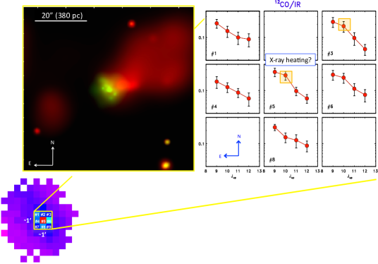
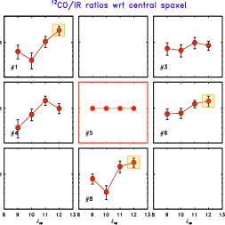
Figure 10: Bottom left: SPIRE SSW ¹²CO emission maps showing the nine spaxels involved in the analysis. Top left: Hard (green) and soft (red) X–ray emission from Chandra from Marinucci et al. (2012) of the outflow observed in the central region ($\sim$1^′$\times$1^′) in NGC 4945. Middle:¹²CO/IR results obtained using SSW SPIRE data (19″ beam) numbered following the scheme shown in the bottom left panel. Right: ¹²CO/IR results normalized to the emission of the central spaxel (red square).

5.4 Heating and density distribution at small scales ($\lesssim$200 pc) using PACS

We now focus our attention to the ¹²CO emission observed at higher frequencies with PACS. At this resolution (9.4″) we are covering spatial scales of the order of $\lesssim$200 pc. The observed PACS spectra along with the simulated LTE results obtained with MADCUBA are shown in Fig. 12. From the rotational diagrams (Fig. 13) we obtained the T_ex and N_mol for each spaxel. From this analysis we found that the highest temperatures (846 K and 871 K) are not found in the nucleus but in two spaxels located closed to the nucleus in the northern and southern spaxels. They are mainly located in the disk plane of the galaxy. On the other hand, the nucleus is characterized by T_ex$\sim$360 K. Above and below the disk plane lower T_ex are found (from $\sim$240 K up to $\sim$330 K).

According to this result, mechanical heating seems the most probable mechanism able to explain the spatial distribution of the excitation temperature at this scale. Indeed, if the X–ray emission were dominating the nuclear region one would have expected the highest excitation temperature in the nucleus. In order to exclude the presence of a XDR in the central spaxel, we derived the intrinsic excitation temperature, correcting the observed T_ex for the nuclear extinction. We thus apply the extinction law:

$$\hskip 2.84526ptI^{int}_{\lambda}=I^{obs}_{\lambda}\times e^{\tau_{\lambda}},$$ (5)

where $\tau_{\lambda}$ can be derived following the relation:

$$\hskip 2.84526pt\tau_{\lambda}=\tau_{100\mu m}\times\left(\frac{100\hskip 2.84526pt\mu m}{\lambda}\right)^{\beta}.$$ (6)

The optical depth $\tau_{100\mu m}$ is derived at 100 $\mu$m from the continuum SED fitting (i.e., $\tau_{100\mu m}\sim$1.2) with $\beta$=2.0 (§ 3.2), assuming that the gas is homogeneously mixed with the dust. For each PACS spectrum of the nuclear spaxel we applied the extinction law associated to the specific wavelength. The corrected excitation temperature of the central spaxel is $\sim$470 K, far below the values obtained in the surrounding regions ($\sim$850 K). We then conclude that the dust opacity does not play an important role in our conclusions. Even the AGN interaction does not seem to have a strong impact on the thermal structure of the source at large spatial scales.

According to the results obtained from large to small scales we summarize the distribution of T_ex in Fig. 14 (top panel). The excitation temperature distribution of PACS data is in good agreement with that derived using SSW SPIRE data.

For what concerns the molecular column density N_CO, the highest values are found in the nucleus corresponding to moderate excitation temperatures, while lower column densities are found in correspondence of maximum temperatures in the disk. In Fig. 14 (bottom panel) we reported the distribution of N_CO at different spatial scales.

In Tab. 9 we summarize all the excitation temperature T_ex and column density N_CO values derived at different spatial scales.

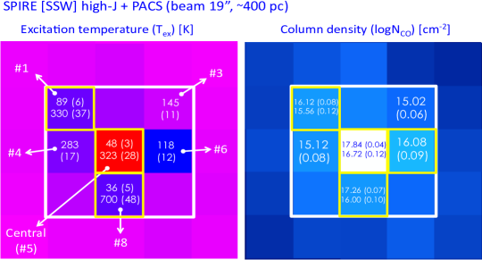
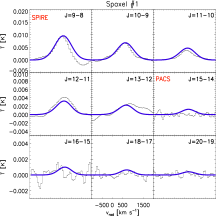
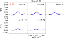
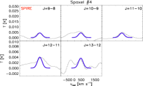
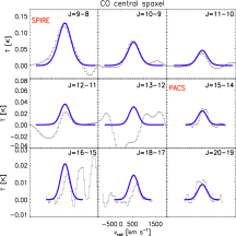
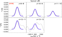
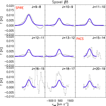
Figure 11: LTE results derived combining SSW SPIRE and PACS spectra. Top: Distribution of the excitation temperature (T_ex, top left) and column density (N_CO, top right) derived applying MADCUBA to the combined SSW SPIRE and PACS spectra. The FoV covered by 3$\times$3 spaxels ($\sim$1′$\times$1′) is the same than that shown in Fig. 10. Bottom: Observed (black) and simulated (blue) ¹²CO emission spectra from combining SSW SPIRE and PACS. The spaxels are identified using the same number used in the top panel. For the spaxel #3 and #6 only SPIRE data are available while for the spaxels #1, #5 (central) and #8 SSW SPIRE and PACS data are combined together. The ¹²CO emission is found in the inner region (3$\times$3 spaxels) and mainly located in the disk, with some contribution in the perpendicular direction.

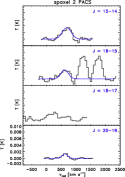
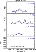
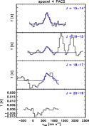
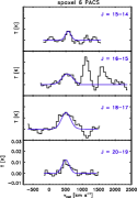
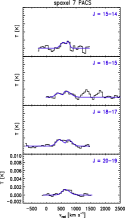
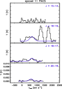
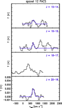
Figure 12: Left: Observed ¹²CO PACS spectra (black) along with the simulated Gaussian fit results (blue). For each spectrum the respective rotational transition (J+1 $\rightarrow$ J) is shown. The flux emission is shown in main beam temperature (T_MB). The OH emission lines close to the ¹²CO(16–15) transition are also observed (see Fig. 9).

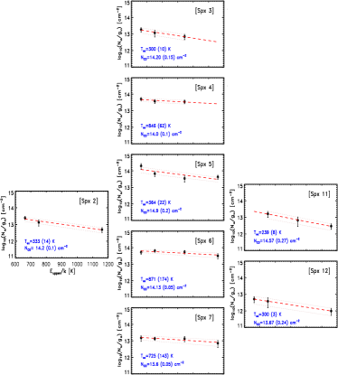
Figure 13: Rotational diagrams derived for PACS data. The excitation temperatures (T_ex) and the (logarithmic) column densities (N_CO) with their respective uncertainties are derived for each spaxel.

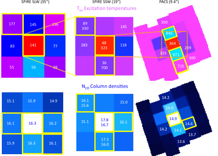
Figure 14: Excitation temperature and (logarithmic) column density distributions at different spatial scales as derived using SPIRE (SLW, SSW) and PACS data. The yellow squares identify the spaxels with high values for each parameter.

Table 9: Summary of the several T_ex and N_CO values derived for the ¹²CO molecule at different resolutions.

Spatial scale	Spatial resolution	Instrument	Jup levels	Number of	Tex	NCO	Figure/
	(arcsec, pc)			Components	(K)	(cm-2)	Table
(1)	(2)	(3)	(4)	(5)	(6)	(7)	(8)
Intermediate	20″, $\lesssim$ 400	APEX, HIFI	3 $\rightarrow$ 9	2	17, 90	17.6, 16.7	F5/T8
Large	35″, $\lesssim$ 700	SPIRE SLW & SSW	4 $\rightarrow$ 13	1 (2a)	141	16.3	F8, F14
Large–intermediate	35″, $\lesssim$ 700	SPIRE SLW & SSW, PACS	4 $\rightarrow$ 20	2	82, 330	$\sim$17, 16.7	F9
Intermediate	19″, $\lesssim$ 400	SPIRE SSW, PACS	9 $\rightarrow$ 20	2	48, 323	17.8, 16.7	F11, F14
Small	9.4″, $\lesssim$ 200	PACS	15 $\rightarrow$ 20	1	364 (470b)	14.9 (14.86)	F12, F13, F14

Notes: Column (1-2): Spatial scale and spatial resolution of the data analyzed; Column (3): instrument with which the analysis has been performed; Column (4): (upper) rotational transition J_up range involved in the analysis accordingly to the instruments considered, listed in Col. (3); Column (5): number of components (i.e., c) used in the fit; Column (6): excitation temperature of ¹²CO molecule in kelvin; Column (7): column density of ¹²CO molecule in cm^-2; Column (8): figure (F) and/or table (T) showing the results in each specific case; (a) see § 5.1 for details; (b) see § 5.3 for details.

5.5 The dust and gas in a multi–phase ISM

The trend we found in our ¹²CO column densities, N_CO, as a function of the rotational levels J involved in the LTE analysis shows, as expected from a multi–phase molecular clumpy medium, a gradient in both the H₂ density, the kinetic temperature and a decreasing column density of the hot gas at increasing J. As the quantum number J of the transitions used in the analysis increases, the physical conditions required for their excitation change according to their critical densities and the energy above the ground state of the levels involved in our study. In fact, we see large changes in temperature from 20 K for the mid J to 400 K for the high J (see Tab. 9). This is consistent with the picture of the multi–phase molecular ISM described above. Therefore, the ¹²CO column densities, N_CO, will decrease from the HIFI to the PACS data analysis since the amount of dense and hot gas measure by the high-J is much smaller than the cold-warm gas measure from the low-J.

We could use the ratios between the column densities from the different instruments to roughly estimate the fraction of the warm-hot molecular component to the cold component. In particular, the cold–warm component at $\sim$20 K is characterized by N(¹²CO_cold-warm) = 10^17.6 cm^-2, the warm component at 90 K shows N(¹²CO_warm) $\lesssim$ 10¹⁷ cm^-2 while the hot component at $\sim$370 K is characterized by N(¹²CO_hot)$\sim$10¹⁵ cm^-2. In addition, the coldest component traced by the J=1–0 and J=2–1 transitions have a ¹²CO column density of 9.6$\times$10¹⁸ cm^-2 for a source size of 20″$\times$20″(Wang et al. 2004), about one order of magnitude larger than the cold–warm component. Thus, the ratio between the cold–warm (CW) and hot (H) components with respect to the cold (C) component is CW/C=0.05 and H/C=10^-4: these values correspond to larger column density of the cold–warm component with respect to the hot component (CW/H) of a factor of $\sim$500.

From our results we can also estimate the total molecular hydrogen column densities, N(H₂). From the SED fitting analysis we derived a total molecular of 7.6 10⁸ M_⊙ for the typical GDR = 100. Then, the N${}_{H_{2}}$ obtained for the size of the dust emission of 20″$\times$10″ corresponds to N${}_{H_{2}}$$\sim$ 7$\times$10²³ cm^-2. To properly account for the total column density N_CO we need to consider the ¹²CO column densities derived for all the components discussed above and scale them (i.e, multiply by a factor of $\sim$2) to the size of the dust emission of 20″$\times$10″. After the correction for the different source sizes, the total ¹²CO column density is of $\sim$2$\times$10¹⁹ cm^-2 which translate into a molecular hydrogen column density of N${}_{H_{2}}$$\sim$ 2$\times$10²³ cm^-2 for the ¹²CO fractional abundance of 10^-4. This is within a factor of $\sim$3 lower than that derived from the SED fitting analysis which is likely within the uncertainties in the sizes, the dust absorption coefficient, the fractional abundance of ¹²CO and the GDR we have considered. Assuming the standard conversion:

$$N_{H_{2}}=9.4\times 10^{20}\hskip 5.69054ptA_{V}\hskip 14.22636pt[cm^{-2}],$$ (7)

from Bohlin et al. (1978) (see also Kauffmann et al. 2008; Lacy et al. 2017), we derive very large visual extinction in both cases ($>$200 mag) as a results of the derived column densities.

We thus find that the hydrogen column densities derived from the SED fitting approach and ¹²CO analysis are in good agreement. These values are higher than those derived for some local AGN and starburst dominated galaxies like NGC 1068 (García-Burillo et al. 2014; Viti et al. 2014) and NGC 253 (Pérez-Beaupuits et al. 2018), but similar to those derived for Compton-thick type 2 Seyfert galaxies like Mrk 3 and NGC 3281 (Sales et al. 2014).

Furthermore, the typical molecular fractional abundances observed in starburst galaxies derived using high density gas tracers like [HCN]/[H₂] (=X_HCN) is of the order of 10^-8 (see Wang et al. 2004; Martín et al. 2006). The derived column densities between ¹²CO and HCN from our LTE analysis are of the order of N_CO/N_HCN $\sim$10¹⁷/10¹³$\sim$10⁴. This is the same ratio than that obtained when considering the fractional abundances relative to H₂, X_CO = 10^-4 and X_HCN = 10^-8 (see Martín et al. 2006).

6 Discussion

6.1 Gas heating mechanisms

Distinguishing among the heating mechanisms, like photoelectric effect by UV photons (PDRs) or XDRs and mechanical processes (like shocks, stellar winds, outflows) is not straightforward, and in most cases a number of mechanisms coexist with different contributions depending on the spatial scale. Many works have addressed this issue modeling the effect of different mechanisms and comparing the predictions with ¹²CO observations of galaxies with different type of activity like starburst galaxies, as M82 (Panuzzo et al. 2010; Kamenetzky et al. 2012) and NGC 253 (Rosenberg et al. 2014a; Pérez-Beaupuits et al. 2018), AGN-dominated galaxies, as NGC 1068 (Spinoglio et al. 2012; Hailey-Dunsheath et al. 2012) and Mrk 231 (van der Werf et al. 2010; Mashian et al. 2015), and composite AGN-SB galaxies, like NGC 6240 (e.g., Meijerink et al. 2013). The ¹²CO emission is strongly affected by the specific mechanism(s) (or by the combinations of them) at work in each galaxy. Some differences can be highlighted between them. When PDRs dominate the emission, the ¹²CO emission increases up to rotational transition J_up=5 and then decreases. In presence of XDRs or shocks the contribution of the ¹²CO emission increases up to high (J${}_{up}>$10) frequencies.

The ¹²CO Spectral Line Energy Distribution (hereafter, ¹²CO SLED) for a large variety of systems has been used in literature as a powerful tool to derive the physical parameters characterizing the molecular gas phase. In Fig. 15 (left panel) the ¹²CO SLEDs for different kind of galaxies are shown. Most of the ¹²CO fluxes shown in Fig. 15 (left panel) are taken from the work by Mashian et al. (2015) (and references therein). This plot can be used for direct comparison of the ¹²CO SLEDs of the different systems up to high J transitions.

We have selected three different kinds of galaxies: (1) AGN-dominated, (2) SB-dominated and (3) AGN-SB composite galaxies. Among the AGN-dominated systems, we selected the prototype (Sy2) NGC 1068 and (Sy1) Mrk 231. The former shows strong ¹²CO line emission above J_up=20 while Mrk 231 shows a ¹²CO SLED shape relatively flat for the higher–J transitions. In both cases, Mashian et al. (2015) and van der Werf et al. (2010) claimed that the results are consistent with the presence of a central X–ray source illuminating the circumnuclear region. Hailey-Dunsheath et al. (2012) also found that in NGC 1068 the gas can be excited by X–rays or shocks although they could not be able to differentiate between the two. As starburst galaxies, we selected M82 and NGC 253. In M82 Panuzzo et al. (2010) found that the ¹²CO emission peaks at J_up = 7, quickly declining towards higher J. They argued that turbulence from stellar winds and supernovae may be the dominant heating mechanism in this galaxy. Rosenberg et al. (2014a), studying NGC 253, concluded that mechanical heating plays an important role in the gas excitation although heating by UV photons is still the dominant heating source. The results from Pérez-Beaupuits et al. (2018) are also in agreement with those presented by Rosenberg et al. (2014a). Finally, the AGN-SB composite galaxy NGC 6240 has been selected. Its ¹²CO SLED shows a similar shape to that of Mrk 231 but this is characterized by clear evidence of both shocks and mechanical heating (Meijerink et al. 2013).

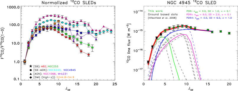
Figure 15: Left: Comparison of ¹²CO SLEDs (normalized to the ¹²CO(1-0) flux of each specific source) obtained from different sources. Starburst (SB), AGN and composite (AGN-SB) sources have been considered. A ¹²CO SLED of a sub-millimeter galaxy (SMG) at high-z analyzed by Cañameras et al. (2018) has been also shown. Different colors identify the galaxies while different symbols the types of object. In each group the following galaxies have been selected: M82 and NGC 253 as starburst, NGC 6240 and NGC 4945 as AGN-SB composite galaxies and NGC 1068 and Mrk 231 as AGN-dominated galaxies. The galaxy G244.8+54.9 has been chosen as representative of SMG at high-z, for which the authors derived log n_gas$\sim$5.1 cm^-3 and log G₀$\sim$3.7 (Habing units). Right: Results of the ¹²CO SLED of NGC 4945 from J = 1–0 through 20–19 applying the Kazandjian et al. (2015) mechanical heating models. The black points are the observed ¹²CO fluxes obtained from ground based observations (Hitschfeld et al. 2008) while in green are the data from this work. The fit was constrained to three PDR models, all of them with some contribution of mechanical heating (mPDR), displayed in green, magenta and blue. Dashed gray lines show the other best fit results for the three PDRs. The dashed blue line is also shown to represent a model with the same n_gas and G₀ parameters as those characterizing the PDRIII model but with no mechanical heating contribution ($\alpha$=0). The red line represents the best fit with the minimum $\chi^{2}_{red}$ ($\sim$0.8) while the light red area shows the combination of other best fits with slightly higher $\chi^{2}$ ($<$1.4). The H₂ density (i.e., n_gas in log cm^-3), G₀ (log Habing flux) and percentage of mechanical heating $\alpha$ values are shown in the legend for the three best fit components.

We then derived the ¹²CO SLED for our AGN-SB composite galaxy NGC 4945 (Fig. 15). Comparing the different ¹²CO SLEDs normalized to the ¹²CO(1-0) flux of each individual galaxy, NGC 4945 seems to show a behavior similar to that found in Mrk 231 (AGN-dominated object) and M82 (SB galaxy) up to J_up$\sim$8, then resembling to Mrk 231 at 8$<$J_up$<$13, finally showing a trend in between that shown by Mrk 231 and NGC 6240 (AGN-SB galaxy) at 14$<$J_up$<$20. The similarity of the ¹²CO SLED shape at higher J transitions with those characterizing Mrk 231 and NGC 6240 provides clues on the presence of X–ray or shocks mechanisms dominating at higher frequencies.

6.2 The dominant heating in NGC 4945

In order to quantify the contribution of the different heating mechanisms in NGC 4945 we applied the Kazandjian et al. (2015) models to investigate the effects of mechanical heating on molecular lines. According to their models the authors found that the emission of low-J transitions alone is not good enough to constrain the mechanical heating (hereafter, $\Gamma_{mech}$) while the emission of ratios involving high-J (and also low-J) transitions is more sensitive to $\Gamma_{mech}$. The strength of $\Gamma_{mech}$ is parametrized by using the parameter $\alpha$, which identifies the ratio between the mechanical heating, $\Gamma_{mech}$, versus the total heating rate at the surface of a pure PDR (no mechanical heating applied), $\Gamma_{surf}$. This can assume values between 0 and 1. In particular, $\alpha$ = 0 corresponds to the situation in which no mechanical heating is present in the PDR, while $\alpha$ = 1 represents the model where the mechanical heating is equivalent to the heating at its surface (see Rosenberg et al. 2014a; Kazandjian et al. 2015). In their models, they assume that mechanical feedback processes like young stellar object (YSO) outflows and supernovae (SNe) events are able to heat the dense molecular gas. The former injects mechanical energy into individual clouds, while the latter injects mechanical energy into the star-forming region amongst the PDR clouds, by turbulent dissipation. The mechanical energy liberated by these events is then deposited locally in shock fronts (see Loenen et al. 2008; Kazandjian et al. 2015).

For NGC 4945 we considered the observed ¹²CO fluxes up to J_up=16 (PACS data). In order to properly constrain the ¹²CO SLED, we complement our SPIRE and PACS data with ground based data obtained by Hitschfeld et al. (2008) al lower J transitions (J$\leq$4) using NANTEN2. The angular resolutions used in their work for the ¹²CO transitions from J_up=1 to 4 vary from 45″ to 38″ (see Tab. 2 in their work). We scaled all these data using the largest angular resolution of 35″ as derived from the Herschel data.

The model which better reproduces our data has been identified by the use of the minimum reduced chi-square value ($\chi^{2}_{red}\sim$0.8). The results are shown in Fig. 15 (right panel). According to the best fit result we found that NGC 4945 is characterized by medium-high gas density (log n_gas = 3.0-5.0 cm^-3) and FUV incident flux, G₀, ranging from 10 up to 10⁶. We properly fit the observed ¹²CO emission using three PDR functions (mPDRI, mPDRII, mPDRIII), all of them needing additional mechanical heating. Two of them (mPDRI, mPDRII) have $\alpha$=0.1 while the third model (mPDRIII) has $\alpha$ = 1.0 (or 0.75 according to the second best fit value). For mPDRI the $\alpha$ value translates into $\Gamma_{mech}$$\sim$4$\times$10^-24 erg s^-1 cm^-2 while mPDRII is characterized by $\Gamma_{mech}$$\sim$3$\times$10^-20 erg s^-1 cm^-2. For mPDRIII the highest mechanical heating is achieved, $\Gamma_{mech}$$\sim$5$\times$10^-19 erg s^-1 cm^-2. According to these results, it is apparent that mechanical heating is needed to reproduce the observed data. Indeed, in contrast to the results derived for the starburst galaxies NGC 253 (Rosenberg et al. 2014a; Pérez-Beaupuits et al. 2018) and Arp 299 (Rosenberg et al. 2014b), the shape of the ¹²CO ladder of NGC 4945 is flatter at higher J transitions (PACS; left panel in Fig. 15). In our case the contribution of shocks (or turbulent) heating is the main source of excitation for ¹²CO emission at J${}_{up}>$ 9–10. On the other hand, photoelectric heating seems to be the main source of heating at low and mid-J transitions (J${}_{up}<$10).

These results confirm that at a resolution of 35″ physical processes like turbulent motions or shocks are able to excite the gas mechanically in the central region of NGC 4945. In the next section we propose a plausible interpretation of the mechanical heating able to explain the emission of the high-J ¹²CO lines detected with PACS.

From the work by Cañameras et al. (2018) a sample of sub-mm galaxies at high-$z$ has been analyzed deriving the G₀ and n_gas parameters. For their sample they derived a typical gas density and a FUV radiation field in the range log n_gas$\sim$4-5.1 cm^-3 and log G₀$\sim$2.2-4.5 (in ‘Habing units’), comparing their values with those derived for normal star-forming galaxies for which derive log n_gas=2-4 cm^-3 and log G₀$\sim$2.5-5 (in ‘Habing’ units) (Malhotra et al. 2001) and local ULIRGs, with log n_gas=4-5 cm^-3 and log G₀$\sim$3-5 (in ‘Habing’ units) (Davies et al. 2003). The values shown in Fig. 9 in their work can be used to compare our results with those obtained for these samples. For instance, in the case of the starburst galaxy NGC 253 (Rosenberg et al. 2014a), a (mean) density of log n_gas$\sim$5.1 cm^-3 and FUV radiation field log G₀$\sim$5.0 can be derived. For NGC 4945, we ended up with (mean) values of log n_gas$\sim$4.6 cm^-3 and log G₀$\sim$5.5. Our results place NGC 4945 in the region covered by local starburst galaxies (as NGC 253) and ULIRGs with similar density but characterized by higher FUV radiation.

From Hollenbach et al. (1991) we are also able to derive a first-order estimate of the incident FUV flux radiation, G₀, assuming FUV heating from the dust properties derived in § 3.2 following the equation:

$$\hskip 8.53581ptG_{0}=3.7\times 10^{-3}\hskip 5.69054pt\tau_{100\mu m}\hskip 5.69054ptT_{dust}^{5}.$$ (8)

We used the opacity $\tau$ computed at 100 $\mu$m ($\tau_{100\mu m}$$\sim$1.2) estimated from the SED fitting assuming that the dust temperature is similar to the equilibrium dust temperature at the surface of the emitting region. According to the SED fitting results (§ 3.2), we ended up with two dust temperature components from which we derived log G₀$\sim$5.8, similar (slightly higher) to that found for the cold component in NGC 253 (i.e., log G₀$\sim$5.5; see Pérez-Beaupuits et al. 2018) and consistent with that found from the models ($\sim$5.5).

On the other hand, the n_H2 densities derived from the LTE and LVG models applied to the ¹²CO molecule using HIFI and APEX data are in between n${}_{H_{2}}$$\lesssim$10⁴-10⁵ cm^-3. These values are in good agreement with the densities derived with the PDR model (n_H2$\sim$10³-10⁵ cm^-3).

6.2.1 Mechanical heating: the bar potential

According to the results derived in the 2D thermal structure analysis performed at different spatial scales (from $\lesssim$200 pc to 2 kpc) focusing on the emission of the ¹²CO molecule from the J = 4–3 to 20–19 we can summarize what follows for the four regions:

$\bullet$

700 pc--2 kpc: The ¹²CO/IR ratios of the low-J lines (J_up$<$10) is larger by a factor of $\lesssim$2 in the inner 700 pc than in the surrounding region (2 kpc). However, for mid-J lines (J_up=11–13), the ¹²CO/IR values are similar in both regions;

$\bullet$

Inner 700 pc: The LTE analysis of the inner 700 pc, which includes the whole range of ¹²CO lines (from J_up=4 to 20), shows that the ¹²CO emission can be explained by a two components model with temperatures of 80 K and 330 K and source size of about 20″ (400 pc) and 7″ ($\sim$150 pc), respectively;

$\bullet$

360 pc--1 kpc: The ¹²CO/IR ratios peak at the mid–J (J_up=9, 10) lines in the central and north-west spaxels: this is in very good agreement with the distribution of the X–ray outflow (i.e., perpendicular – north-west direction – to the disk of the galaxy). Normalizing for this contribution, we derived increased ¹²CO/IR ratios for the highest mid–J lines (J_up=11 and 12) in the ring structure, in particular along the galaxy plane and toward the west. This result lets us argue that shocks probably dominate at these frequencies;

$\bullet$

Inner 200 pc--360 pc: The LTE analysis of the high-J ¹²CO lines confirmed the trend found at larger scales. The highest temperatures ($\sim$560 K) are found around the nucleus (T$\sim$360 K, after correcting for the nuclear extinction), in the north–south direction along the galaxy disk.

We thus found a clear trend in the distribution of the excitation temperatures and the ¹²CO/IR ratios. At large scale ($>$700 pc), the highest temperatures are found toward the nucleus and the north, with moderate temperatures in the south. The high temperatures in the north might be related to the large scale X–ray outflow. It is remarkable that, basically at all scales $<$700 pc, the highest temperatures are not found towards the nucleus but toward the disk. Like found at large scale, at intermediate scales (360 pc–1 kpc) we also see high temperatures in the direction of the X–ray outflow. At the smallest scales ($\sim$200 pc), we clearly see that even if the largest column density is found in the nucleus, the highest temperatures are found in the disk.

This result is an agreement with that derived by Lin et al. (2011). In their work the authors analyzed in detail the ¹²CO(2–1) emission of the central region (20″$\times$20″) of this galaxy using Submillimeter Array (SMA) data, mainly focusing on its circumnuclear molecular gas emission. They showed that the S-shaped structure of the isovelocity contours can be well reproduced by the bending generated by a shock along the spiral density waves, which are excited by a fast rotating bar. As a result, their simulated density map reveals a pair of tightly wound spirals in the center which pass through most of the ring-like (claimed to be a circumnuclear starburst ring by other authors) high-intensity region as well as intersect several Pa$\alpha$ emission line knots located outside the ring-like region (Fig. 16). According to their scenario, the inner region of NGC 4945 is characterized by high column density surrounded by lower values in the nearby spaxels. As shown in Fig. 16, at high density regions correspond low temperatures, and vice versa, in very good agreement with our PACS results.

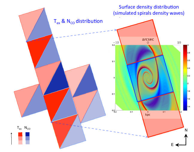
Figure 16: Comparison between the results obtained at small scales using PACS (left) with those derived in Lin et al. (2011) (right). Left: Excitation temperature (T_ex; red colors) and column density (log N_CO; blue colors) values derived using PACS data for the inner spaxels. The highest temperatures are found in correspondence of the two spaxels closed to the nucleus, in the northern and southern directions, while the peak in the column density is found in the central spaxel. Right (back): Simulated spiral density waves overplotted to the velocity structure (Lin et al. 2011) in a FoV of 20″$\times$20″. High density values are in red while lower values are in blue. Right (front): Corresponding PACS spaxels overplotted onto the same FoV to show the respective excitation temperature distribution derived from PACS data. Higher values of the simulated density map reveal a pair of tightly wound spirals in the center which correspond to the highest N_CO and lower T_ex in PACS data. On the other hand, lower values in the surface density correspond to higher T_ex and lower N_CO according to PACS. North is at the top and East to the left.

Our data does not have the high angular resolution required to reveal the distribution of the thermal structure of this region. However, Henkel et al. (2018), using ALMA data, found a good agreement with the simulated results presented by Lin et al. (2011). As mentioned in §1, Henkel et al. (2018) found the presence of a dense and dusty nuclear disk (10″$\times$2″) which encloses an unresolved molecular core with a radius $\lesssim$2″ (of the same size as the X–ray source observed with Chandra). At scales larger than those shown by Lin et al. (2011), Henkel et al. (2018) also observed the presence of two bending spiral-like arms (one in the west turning toward the north-east and one in the east turning toward the south-west) at a radius of $\sim$300 pc ($\sim$15″) from the center. The arms are connected through a bar-like structure with a total length $\lesssim$ 20″ along the east-west directions. They also suggested the presence of an inflow of gas from 300 pc down to 100 pc through the bar (see Fig. 26 in their work).

At the spatial scales sampled by our data, we found good agreement between the presence of a bar-like structure and tightly wound spiral arms (see Ott et al. 2001; Chou et al. 2007; Lin et al. 2011; Henkel et al. 2018) and our results. Accordingly, the mechanical heating produced by shocks, possibly driven by the outflow and by the bar potential, dominates in NGC 4945 at scales $\lesssim$20″ ($\lesssim$360 pc).

6.3 Dust heating

Understanding the nature of the source that heats the dust in the nuclear regions of NGC 4945 is a topic under discussion. Many works suggested that the circumnuclear starburst, rather than the AGN activity, is the primary heating agent of the dust.

From the work by Brock et al. (1988), we know that $\lesssim$80% of the total infrared emission of this object is enclosed in a region no larger than $<$12″$\times$9″. This size is comparable to the continuum source we derived from the multi-wavelength SED fitting analysis (20″$\times$10″) and characterized by two dust temperatures of 28 and 50 K. Within this area we found a total mass of dust of $\lesssim$10⁷ M_⊙, in agreement with previous works (Weiß et al. 2008; Chou et al. 2007). The dust temperature we obtained is lower than the excitation temperature of the mid-J ¹²CO, characterized by energies from 55 K to 500 K above the ground state, as expected from mechanical heating.

Similar continuum source size at millimeter wavelengths have been derived from the works by Chou et al. (2007) and Bendo et al. (2016). Chou et al. (2007) derived a deconvolved continuum source size of 9.8″$\times$5.0″ at 1.3 mm and slightly smaller ($\sim$7.6″$\times$2.0″) at 3.3 mm. These emissions are not aligned either with the starburst ring or with larger galactic disk, observed in Pa$\alpha$ by Marconi et al. (2000).

The size of the continuum source derived at centimeter wavelengths is much smaller (i.e., 7.4″$\times$3.4″ at 21 cm) than that measured at 1.3 mm. Furthermore, the centimeter continuum source size and inclination are comparable with those of the starburst ring (i.e., $\sim$5″ or 100 pc-scale and position angle $\sim$45 degree). They proposed that at cm wavelengths the star formation activity (as supernovae events) in the starburst ring can produce the nonthermal (synchrotron) emission which dominates at these wavelengths. Chou et al. (2007) conclude that the dust emission dominates at 1.3 mm (and at 3.3 mm, with a radius of 4.9″), mainly heated by the star formation activity. The different origin of the dust emission at mm and cm wavelengths help us to understand the different continuum source sizes obtained.

On the other hand, Bendo et al. (2016) analyzed the continuum emission at 85.69 GHz ad the H42$\alpha$ emission line deriving comparable size ($\sim$7″$\times$1.7″) with those measured by previous works at similar frequencies and emission lines (Ott et al. 2001; Cunningham & Whiteoak 2005; Roy et al. 2010). They support the hypothesis that if the gas around the nucleus would be photoionized by the AGN they would expect to see a central peak excess in their exponential disk model (with scale length of 2.1″). Indeed, the spatial extent of the emission derived in their work, the absence of the peak excess and of any broad line emission suggest that both (continuum and line) emissions originate from the gas photoionized from the circumnuclear starburst, not from the AGN.

Our results suggest that star formation (in the circumnuclear starburst) is the main driving activity able to heat the dust. Unfortunately our data does not have the high angular resolution required to reveal the distribution of the thermal structure of the inner region. Continuum observations at higher angular resolutions as those feasible by using the Stratospheric Observatory For Infrared Astronomy (SOFIA; Young et al. 2012) airborne observatory are required to obtain photometric measurements of the dust continuum in the far-IR in order to disentangle and to characterize the contributions produced by the starburst and the central AGN, respectively.

7 Summary and conclusions

Using data from the HIFI, SPIRE and PACS instruments onboard the Herschel satellite and APEX we have been able to study the properties of the molecular ISM in the nearby galaxy NGC 4945, a remarkable prototype of AGN-SB composite galaxy. The spectroscopy data presented in this paper includes a combination of low and high density molecular gas tracers such as the ¹²CO, ¹³CO, HCN, HNC, CS, [CI], HCO⁺ and CH. The main focus of the paper is to study the spatial distribution of ¹²CO emission over a large frequency range covering transitions from J= 3–2 to 20–19 combining all data available from the instruments mentioned above. We also preset the Spectral Energy Distribution (SED) of the dust continuum emission from 20 $\mu$m to 1.3 mm.

Under the assumption of the local thermal equilibrium (LTE analysis, using MADCUBA) excitation, we derived the excitation temperature T_ex and the molecular column density N_mol for ¹²CO, ¹³CO, HCN, HNC, CS, [CI], HCO⁺ and CH combining HIFI and, when available, APEX data. The highest column densities are found for ¹²CO, ¹³CO and [CI], ranging between log N_mol $\sim$ 16.5-17.5 cm^-2. For the remaining molecules we derived a column density in the range log N_mol=13-14 cm^-2 and T_ex between 20-30 K. According to the non-LTE approach (using RADEX) we derived moderate volume gas densities, with n(H₂) in the range 10³-10⁶ cm^-3. Lower values are derived for ¹²CO, ¹³CO and [CI] while higher values are obtained for the high density gas tracers such as HCN, HNC, HCO⁺ and CS. From the low and high density tracers we derived in NGC 4945 gas volume densities (10³–10⁶ cm^-3) similar to those found in other galaxies with different type of activity.

We used the SPIRE and PACS spectroscopic data applying the LTE (multi-line transitions) analysis to derive the thermal and column density structures of the molecular gas ¹²CO for scales raging from $<$200 pc up to 2 kpc. We also analyzed the ¹²CO Spectral Line Energy Distribution (SLED) applying the Kazandjian et al. (2015) models.

The main results can be summarized as follow:

$\bullet$

At large scale (700 pc–2 kpc), as obtained from SLW SPIRE, we derived that high temperatures are mainly found in the northern part of the galaxy as well as in the disk plane. This suggests the presence of the outflow might affects the temperature observed in the north-west direction. The column densities are higher in the center and towards the south direction;

$\bullet$

At intermediate scales (360 pc–1 kpc), as those obtained from the SSW SPIRE data, the heating is distributed along the disk plane and in the south direction too. The column density follows a similar trend than that shown at large scales, characterized by high values in the center and towards the south;

$\bullet$

When moving to smaller scales ($\sim$200 pc), using PACS data, we found a peak in the column density in the central spaxel, surrounded by lower column density but higher excitation temperatures. This result is an agreement with that derived by Lin et al. (2011) . They proposed the presence of tightly wound spirals in order to explain the distribution of the surface density and the related velocity field in a 20″$\times$20″ region;

$\bullet$

The thermal structure derived from the ¹²CO multi-transition analysis suggests that shocks seem to dominate the heating of the ISM in the nucleus of NGC 4945, located beyond 100 pc from the center of the galaxy. This result is confirmed by the mechanical heating models, which suggest the existence of PDRs but mainly dominated by mechanical heating (i.e., feedback from SNe) in the inner regions of NGC 4945. We proposed that shocks are likely produced by the barred potential and the outflow, observed in the optical and X–ray bands. The high temperatures in the north and north-west directions, found at larger scales, might be related to the outflow;

$\bullet$

The spectral energy distribution (SED) in NGC 4945 has been obtained combining photometric data from far-IR (MSX, PACS and SPIRE) and sub-mm (LABOCA) and mm (SMA) data. From the SED fitting analysis we derived that the source is resolved at these wavelengths. We found good results when two modified black body functions are considered, characterized by a cold (T$\sim$28 K) and a warmer temperature component of 50 K and a source size of $\Omega_{s}$=20″$\times$10″. Assuming a gas-to-dust ratio between 100 and 150, we derived in NGC 4945 a total gas mass in the range $\sim$8–11$\times$10⁸ M_⊙ in a region of 40″$\times$40″. This result is consistent with the gas mass estimations derived in previous works (Weiß et al. 2008);

$\bullet$

The hydrogen column density derived from the SED fitting is in good agreement with that derived by Wang et al. (2004) using ¹²CO(1–0) and ¹²CO(2–1) transitions. NGC 4945 is characterized by N(H₂)$\sim$5$\times$10²³ cm^-2: this value is larger than those obtained for local starburst galaxies (e.g., NGC 253) and similar to those obtained for Compton-thick Seyfert 2 galaxies.

The results obtained in this work seem to confirm that the presence of the AGN in NGC 4945 has little impact on the thermal properties of its nuclear starburst. IR observations at higher spatial resolution are required to characterize both the dust and molecular line emissions. Spectroscopic and photometric observations like those could be achieved by the instruments onboard SOFIA (e.g., HAWC$+$, CASIMIR and/or GREAT) are needed in order to characterize the physical conditions of temperature and density as well as the structure of the emission itself in the very inner regions of NGC 4945.

Appendix A Deriving the flux density values for the SED fitting analysis

In this appendix we present how the flux densities, used in the SED fitting in § 3.2, are computed for the different wavelengths. The additional data are characterized by different units, we then summarize here the several conversion factors applied to transform the flux densities in Jansky as well as the formula applied for the conversion. In Tab. 10 we show the computed flux density values (with their associated errors), the conversion factors and the pixel sizes for each band.

• For the MSX catalogue we used the following formula:

  $$\hskip 14.22636ptF(40\arcsec)=F_{OBS}\cdot CF\cdot\left(\frac{pixel\hskip 2.84526ptsize}{3600}\frac{2\pi}{360}\right)^{2}.$$ (9)

  The conversion factor (CF) transform the [W m^-2 sr^-2] into [Jy sr^-1] and they have been taken from the website http://irsa.ipac.caltech.edu/applications/MSX/MSX/imageDescriptions.htm.

• Taking into account the LABOCA data from Weiß et al. (2008) we considered the flux density of 15.8 ($\pm$1.6) Jy computed in a beam of 80″$\times$ 80″. From their work we also know that in a beam of 19″$\times$15″ (average beam 17″) the flux density is 7.2 ($\pm$0.8) Jy. If we assume uniform emission outside the beam of 17″ ($<$80″) we are able to compute the flux density in a annular beam with size in between 17″ and 40″:

  $$\frac{(15.8-7.2)[Jy]}{(80^{2}-17^{2})[arcsec]}\cdot(40^{2}-17^{2})[arcsec]=1.85\hskip 2.84526pt[Jy].$$ (10)

  This can be considered a reasonable assumption according to the LABOCA data from which we derived that half of the total flux density emission is enclosed in a beam $\lesssim$20″, while the remaining emission is diluted in the annular beam between $\sim$20″ and 80″.

  Finally, to derive the flux density in a beam of 40″, we added the flux density value obtained in the annular beam to the flux density obtained in a beam of 17″. This gives a total flux density (in a beam of 40″) of 7.2 Jy + 1.85 Jy = 9.05 (1.3) Jy.

Table 10: Flux densities derived from the archive and from the literature for the additional data.

Data	band	Flux	Conversion	Pixel	Ref.
		density	factor	size
	($\mu$m)	(A.U.)		(″)
(1)	(2)	(3)	(4)	(5)	(6)
MSX	21.34	0.27 (0.07)$\times$10-3	2.476$\times$1013	6	a
LABOCA	870	9.05 (1.3)	Eq. 10	–	b

Notes: Column (1): data considered; Column (2): central wavelength of the band; Column (3): flux density (and uncertainty) in the aperture in arbitrary units (see text); Column (4): conversion factor to derive the flux density in Jansky; Column (5): pixel size in arcsec; Column (6): reference considered to get the data: (a) MSX Archive, (b) Weiß et al. (2008).

References

- Alatalo et al. (2011) Alatalo, K., Blitz, L., Young, L. M., et al. 2011, ApJ, 735, 88
- Bendo et al. (2016) Bendo, G. J., Henkel, C., D’Cruze, M. J., et al. 2016, MNRAS, 463, 252
- Bohlin et al. (1978) Bohlin, R. C., Savage, B. D., & Drake, J. F. 1978, ApJ, 224, 132
- Brock et al. (1988) Brock, D., Joy, M., Lester, D. F., Harvey, P. M., & Ellis, Jr., H. B. 1988, ApJ, 329, 208
- Cañameras et al. (2018) Cañameras, R., Yang, C., Nesvadba, N. P. H., et al. 2018, A&A, 620, A61
- Cherednichenko et al. (2002) Cherednichenko, S., Kroug, M., Merkel, H., et al. 2002, Physica C Superconductivity, 372, 427
- Chou et al. (2007) Chou, R. C. Y., Peck, A. B., Lim, J., et al. 2007, ApJ, 670, 116
- Chung et al. (2011) Chung, A., Yun, M. S., Naraynan, G., Heyer, M., & Erickson, N. R. 2011, ApJ, 732, L15
- Cicone et al. (2014) Cicone, C., Maiolino, R., Sturm, E., et al. 2014, A&A, 562, A21
- Cresci et al. (2015) Cresci, G., Mainieri, V., Brusa, M., et al. 2015, ApJ, 799, 82
- Cunningham & Whiteoak (2005) Cunningham, M. R. & Whiteoak, J. B. 2005, MNRAS, 364, 37
- Curran et al. (2001) Curran, S. J., Johansson, L. E. B., Bergman, P., Heikkilä, A., & Aalto, S. 2001, A&A, 367, 457
- da Cunha et al. (2008) da Cunha, E., Charlot, S., & Elbaz, D. 2008, MNRAS, 388, 1595
- Davies et al. (2003) Davies, R. I., Sternberg, A., Lehnert, M., & Tacconi-Garman, L. E. 2003, ApJ, 597, 907
- de Graauw et al. (2010) de Graauw, T., Helmich, F. P., Phillips, T. G., et al. 2010, A&A, 518, L6
- Done et al. (1996) Done, C., Madejski, G. M., & Smith, D. A. 1996, ApJ, 463, L63
- Flower et al. (2010) Flower, D. R., Pineau des Forêts, G., & Rabli, D. 2010, MNRAS, 409, 29
- García-Burillo et al. (2014) García-Burillo, S., Combes, F., Usero, A., et al. 2014, A&A, 567, A125
- Greenhill & Gwinn (1997) Greenhill, L. J. & Gwinn, C. R. 1997, Ap&SS, 248, 261
- Greenhill et al. (1997) Greenhill, L. J., Moran, J. M., & Herrnstein, J. R. 1997, ApJ, 481, L23
- Guainazzi et al. (2000) Guainazzi, M., Matt, G., Brandt, W. N., et al. 2000, A&A, 356, 463
- Güsten et al. (2006) Güsten, R., Nyman, L. Å., Schilke, P., et al. 2006, A&A, 454, L13
- Habing (1969) Habing, H. J. 1969, Bull. Astron. Inst. Netherlands, 20, 177
- Hailey-Dunsheath et al. (2012) Hailey-Dunsheath, S., Sturm, E., Fischer, J., et al. 2012, ApJ, 755, 57
- Henkel et al. (2018) Henkel, C., Mühle, S., Bendo, G., et al. 2018, A&A, 615, A155
- Hildebrand (1983) Hildebrand, R. H. 1983, QJRAS, 24, 267
- Hitschfeld et al. (2008) Hitschfeld, M., Aravena, M., Kramer, C., et al. 2008, A&A, 479, 75
- Hollenbach et al. (1991) Hollenbach, D. J., Takahashi, T., & Tielens, A. G. G. M. 1991, ApJ, 377, 192
- Hopkins et al. (2009) Hopkins, P. F., Hernquist, L., Cox, T. J., Keres, D., & Wuyts, S. 2009, ApJ, 691, 1424
- Itoh et al. (2008) Itoh, T., Done, C., Makishima, K., et al. 2008, PASJ, 60, S251
- Iwasawa et al. (1993) Iwasawa, K., Koyama, K., Awaki, H., et al. 1993, ApJ, 409, 155
- Jackson & Rueda (2005) Jackson, B. & Rueda, P. 2005, in ESA Special Publication, Vol. 589, ESA Special Publication, 66
- Kamenetzky et al. (2012) Kamenetzky, J., Glenn, J., Rangwala, N., et al. 2012, ApJ, 753, 70
- Karachentsev et al. (2007) Karachentsev, I. D., Tully, R. B., Dolphin, A., et al. 2007, AJ, 133, 504
- Kauffmann et al. (2008) Kauffmann, J., Bertoldi, F., Bourke, T. L., Evans, N. J., I., & Lee, C. W. 2008, A&A, 487, 993
- Kazandjian et al. (2015) Kazandjian, M. V., Meijerink, R., Pelupessy, I., Israel, F. P., & Spaans, M. 2015, A&A, 574, A127
- Krugel & Siebenmorgen (1994) Krugel, E. & Siebenmorgen, R. 1994, A&A, 282, 407
- Lacy et al. (2017) Lacy, J. H., Sneden, C., Kim, H., & Jaffe, D. T. 2017, ApJ, 838, 66
- Lin et al. (2011) Lin, L.-H., Taam, R. E., Yen, D. C. C., Muller, S., & Lim, J. 2011, ApJ, 731, 15
- Lisenfeld et al. (2002) Lisenfeld, U., Israel, F. P., Stil, J. M., & Sievers, A. 2002, A&A, 382, 860
- Loenen et al. (2008) Loenen, A. F., Spaans, M., Baan, W. A., & Meijerink, R. 2008, A&A, 488, L5
- Lovas (1992) Lovas, F. J. 1992, Journal of Physical and Chemical Reference Data, 21, 181
- Malhotra et al. (2001) Malhotra, S., Kaufman, M. J., Hollenbach, D., et al. 2001, ApJ, 561, 766
- Maloney (1999) Maloney, P. R. 1999, Ap&SS, 266, 207
- Maloney et al. (1996) Maloney, P. R., Hollenbach, D. J., & Tielens, A. G. G. M. 1996, ApJ, 466, 561
- Marconi et al. (2000) Marconi, A., Oliva, E., van der Werf, P. P., et al. 2000, A&A, 357, 24
- Maret et al. (2011) Maret, S., Hily-Blant, P., Pety, J., Bardeau, S., & Reynier, E. 2011, A&A, 526, A47
- Marinucci et al. (2012) Marinucci, A., Risaliti, G., Wang, J., et al. 2012, MNRAS, 423, L6
- Martín et al. (2019) Martín, S., Martín-Pintado, J., Blanco-Sánchez, C., et al. 2019, A&A, 631, A159
- Martín et al. (2006) Martín, S., Mauersberger, R., Martín-Pintado, J., Henkel, C., & García-Burillo, S. 2006, ApJS, 164, 450
- Mashian et al. (2015) Mashian, N., Sturm, E., Sternberg, A., et al. 2015, ApJ, 802, 81
- Meijerink et al. (2013) Meijerink, R., Kristensen, L. E., Weiß, A., et al. 2013, ApJ, 762, L16
- Meijerink & Spaans (2005) Meijerink, R. & Spaans, M. 2005, A&A, 436, 397
- Meijerink et al. (2006) Meijerink, R., Spaans, M., & Israel, F. P. 2006, ApJ, 650, L103
- Mingozzi et al. (2019) Mingozzi, M., Cresci, G., Venturi, G., et al. 2019, A&A, 622, A146
- Moorwood et al. (1996) Moorwood, A. F. M., van der Werf, P. P., Kotilainen, J. K., Marconi, A., & Oliva, E. 1996, A&A, 308, L1
- Müller et al. (2001) Müller, H. S. P., Thorwirth, S., Roth, D. A., & Winnewisser, G. 2001, A&A, 370, L49
- Nakai (1989) Nakai, N. 1989, PASJ, 41, 1107
- Ott et al. (2001) Ott, M., Whiteoak, J. B., Henkel, C., & Wielebinski, R. 2001, A&A, 372, 463
- Panuzzo et al. (2010) Panuzzo, P., Rangwala, N., Rykala, A., et al. 2010, A&A, 518, L37
- Pérez-Beaupuits et al. (2018) Pérez-Beaupuits, J. P., Güsten, R., Harris, A., et al. 2018, ApJ, 860, 23
- Pickett et al. (1998) Pickett, H. M., Poynter, R. L., Cohen, E. A., et al. 1998, J. Quant. Spec. Radiat. Transf., 60, 883
- Poglitsch et al. (2010) Poglitsch, A., Waelkens, C., Geis, N., et al. 2010, A&A, 518, L2
- Povich et al. (2007) Povich, M. S., Stone, J. M., Churchwell, E., et al. 2007, ApJ, 660, 346
- Puccetti et al. (2014) Puccetti, S., Comastri, A., Fiore, F., et al. 2014, ApJ, 793, 26
- Rivilla et al. (2016) Rivilla, V. M., Fontani, F., Beltrán, M. T., et al. 2016, ApJ, 826, 161
- Rosenberg et al. (2014a) Rosenberg, M. J. F., Kazandjian, M. V., van der Werf, P. P., et al. 2014a, A&A, 564, A126
- Rosenberg et al. (2014b) Rosenberg, M. J. F., Meijerink, R., Israel, F. P., et al. 2014b, A&A, 568, A90
- Roy et al. (2010) Roy, A. L., Oosterloo, T., Goss, W. M., & Anantharamaiah, K. R. 2010, A&A, 517, A82
- Sakamoto et al. (2009) Sakamoto, K., Aalto, S., Wilner, D. J., et al. 2009, ApJ, 700, L104
- Sales et al. (2014) Sales, D. A., Ruschel-Dutra, D., Pastoriza, M. G., Riffel, R., & Winge, C. 2014, MNRAS, 441, 630
- Schurch et al. (2002) Schurch, N. J., Roberts, T. P., & Warwick, R. S. 2002, MNRAS, 335, 241
- Shipman et al. (2017) Shipman, R. F., Beaulieu, S. F., Teyssier, D., et al. 2017, A&A, 608, A49
- Spinoglio et al. (2012) Spinoglio, L., Dasyra, K. M., Franceschini, A., et al. 2012, ApJ, 745, 171
- Spoon et al. (2013) Spoon, H. W. W., Farrah, D., Lebouteiller, V., et al. 2013, ApJ, 775, 127
- Strickland & Heckman (2009) Strickland, D. K. & Heckman, T. M. 2009, ApJ, 697, 2030
- Strickland et al. (2000) Strickland, D. K., Heckman, T. M., Weaver, K. A., & Dahlem, M. 2000, AJ, 120, 2965
- Sturm et al. (2011) Sturm, E., González-Alfonso, E., Veilleux, S., et al. 2011, ApJ, 733, L16
- Swinyard et al. (2010) Swinyard, B. M., Hartogh, P., Sidher, S., et al. 2010, A&A, 518, L151
- van der Werf et al. (2010) van der Werf, P. P., Isaak, K. G., Meijerink, R., et al. 2010, A&A, 518, L42
- Venturi et al. (2017) Venturi, G., Marconi, A., Mingozzi, M., et al. 2017, Frontiers in Astronomy and Space Sciences, 4, 46
- Viti et al. (2014) Viti, S., García-Burillo, S., Fuente, A., et al. 2014, A&A, 570, A28
- Wang et al. (2004) Wang, M., Henkel, C., Chin, Y.-N., et al. 2004, A&A, 422, 883
- Weiß et al. (2008) Weiß, A., Kovács, A., Güsten, R., et al. 2008, A&A, 490, 77
- Wolfire et al. (2010) Wolfire, M. G., Hollenbach, D., & McKee, C. F. 2010, ApJ, 716, 1191
- Young et al. (2012) Young, E. T., Becklin, E. E., Marcum, P. M., et al. 2012, ApJ, 749, L17