Electron-boson-interaction induced particle-hole symmetry breaking of conductance into subgap states in superconductors

Abstract

Particle-hole symmetry (PHS) of conductance into subgap states in superconductors is a fundamental consequence of a noninteracting mean-field theory of superconductivity. The breaking of this PHS has been attributed to a noninteracting mechanism, i.e., quasiparticle poisoning (QP), a process detrimental to the coherence of superconductor-based qubits. Here, we show that the ubiquitous electron-boson interactions in superconductors can also break the PHS of subgap conductances. We study the effect of such couplings on the PHS of subgap conductances in superconductors using both the rate equation and Keldysh formalism, which have different regimes of validity. In both regimes, we found that such couplings give rise to a particle-hole asymmetry in subgap conductances which increases with increasing coupling strength, increasing subgap-state particle-hole content imbalance and decreasing temperature. Our proposed mechanism is general and applies even for experiments where the subgap-conductance PHS breaking cannot be attributed to QP.

I Introduction

Subgap states in superconductors are key features of topological superconducting phases Mourik et al. (2012); Nadj-Perge et al. (2014); Suominen et al. (2017); Nichele et al. (2017); Ménard et al. (2017); Choi et al. (2017); Gül et al. (2018); Deng et al. (2018); Fornieri et al. (2019); Ren et al. (2019); Vaitiekėnas et al. (2020); Wang et al. (2020); Zhang et al. (2021) which offer great promise for quantum information processing Kitaev (2003); Nayak et al. (2008). Tunneling transport into such Andreev bound states (ABSs) provides the most direct and commonly employed method to detect them Law et al. (2009); Flensberg (2010); Wimmer et al. (2011); Setiawan et al. (2015) (Hereafter ABS refers to any subgap state in superconductors.) Most of our understanding of tunneling into superconductors is based on the celebrated Blonder-Tinkham-Klapwijk (BTK) formalism Blonder et al. (1982). One universal consequence of this theory is a precise particle-hole symmetry (PHS) of the conductance into any ABS in a superconductor Lesovik et al. (1997); Wimmer et al. (2011); Martin and Mozyrsky (2014). Specifically, this theory predicts that the differential conductance at a positive voltage $V$ inside the superconducting gap precisely match its counterpart value at $-V$. This symmetry has been shown to be a consequence of the PHS of the mean-field Hamiltonian used in the BTK formalism. However, numerous experiments over two decades Yazdani et al. (1997); Matsuba et al. (2003); Shan et al. (2011); Hanaguri et al. (2012); Suominen et al. (2017); Nichele et al. (2017); Ménard et al. (2017); Choi et al. (2017); Gül et al. (2018); Deng et al. (2018); Chen et al. (2018); Bommer et al. (2019); Chen et al. (2019); Vaitiekėnas et al. (2020); Yu et al. (2021); Saldaña et al. (2020); Farinacci et al. (2020); Wang et al. (2021); Ding et al. (2021) have often observed particle-hole (PH) asymmetric subgap conductances. One way to reconcile this PH asymmetry with the BTK theory is to introduce quasiparticle poisoning induced either by coupling the ABS to a fermionic bath Martin and Mozyrsky (2014); Das Sarma et al. (2016); Liu et al. (2017a) or through a relaxation process from the ABS to the superconductor’s quasiparticle continuum Ruby et al. (2015).

Quasiparticle poisoning (QP) Aumentado et al. (2004); Higginbotham et al. (2015); Albrecht et al. (2017) refers to a process where an electron tunnels from the bulk of the superconductor to an ABS which changes the occupation (parity) of the ABS. Since the parity is used as the qubit state, QP then introduces bit-flip errors Goldstein and Chamon (2011); Rainis and Loss (2012); Budich et al. (2012). Moreover, as QP breaks the PHS of subgap conductances Martin and Mozyrsky (2014); Das Sarma et al. (2016); Liu et al. (2017a), one may be tempted to associate the PH asymmetry to short qubit lifetime. We will show that this correlation is not true in general as contrary to commonly held beliefs, the PH asymmetry can also arise without QP.

In this paper, we propose a generic mechanism for PHS breaking of subgap conductances without changing the superconductor’s parity state, namely, the coupling between ABSs and bosonic modes. While quantum tunneling in dissipative systems has been widely studied Caldeira and Leggett (1983); Ingold and Nazarov (1992), previous works consider coupling between bosonic baths and superconductors without ABSs. Motivated by tunneling experiments into ABSs Yazdani et al. (1997); Matsuba et al. (2003); Shan et al. (2011); Hanaguri et al. (2012); Suominen et al. (2017); Nichele et al. (2017); Ménard et al. (2017); Choi et al. (2017); Gül et al. (2018); Deng et al. (2018); Chen et al. (2018); Bommer et al. (2019); Chen et al. (2019); Vaitiekėnas et al. (2020); Yu et al. (2021); Saldaña et al. (2020); Farinacci et al. (2020); Wang et al. (2021); Ding et al. (2021), here we study tunneling transport from a normal lead into an ABS coupled to bosonic modes, e.g., phonons Shapiro et al. (1975); Friedl et al. (1990), plasmons Hepting et al. (2018), or electromagnetic fields Majer et al. (2007), in the superconductor. Our system has a local fermion parity analogous to the spin-boson model Leggett et al. (1987) with a caveat that our ABSs can participate in transport. Crucially, our study of transport into an ABS coupled to bosonic modes and its relation to PHS breaking of subgap conductances has not been undertaken before. To this end, we present ways to enforce fermion-parity conservation in treating interaction effects on transport into ABSs. We consider two different limits: weak and strong tunneling regimes where the ABS-lead tunnel strength is smaller and larger than the thermal broadening $\sim k_{B}T$, respectively. The weak tunneling limit is studied using the rate equation Mitra et al. (2004); Koch et al. (2004), which is valid for all values of ABS-boson coupling strength where the tunneling rates are calculated using Fermi’s Golden Rule (FGR). In the strong tunneling limit, we study the transport using the Keldysh formalism and treat the ABS-boson coupling within the mean-field approximation.

II Particle-Hole symmetry/asymmetry from Fermi’s Golden Rule

We begin by using FGR to show that while subgap conductances in gapped superconductors (superconductors without baths) preserve PHS even with interactions (including strongly correlated superconductors), the PHS is broken for superconductors with gapless excitations (e.g., phonons, quasiparticles, etc.). The simplest application of FGR Yazdani et al. (1997); Mahan (2000); Balatsky et al. (2006) considers the conductance into an ABS at positive [Fig. 1(a)] and negative subgap energies [Fig. 1(b)] to arise from the tunneling of electrons and holes, respectively, into the ABS (changing the ABS occupancy $n$ from $0\rightarrow 1$). The tunneling rates of electrons [$R^{0\rightarrow 1;e}$ in Fig. 1(a)] and holes [$R^{0\rightarrow 1;h}$ in Fig. 1(b)] can be calculated from FGR to be proportional to the particle and hole component of the ABS wavefunction, respectively. This suggests that the tunneling conductance into an ABS with different weights of particle and hole component is PH asymmetric. However, this simple argument implicitly assumes the presence of QP Martin and Mozyrsky (2014), which empties out the electron from the ABS after each tunneling event such that its occupancy $n$ returns to $n=0$. This implicit assumption can be avoided by taking into account the change in the ABS occupancy $n=0,1$ after each tunneling.

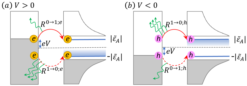
Figure 1: Sequential tunneling from the lead (grey rectangles) to the ABS (blue lines). Tunneling of (a) electrons and (b) holes give rise to current at (a) positive and (b) negative voltages, respectively [Eq. (1)]. The first tunneling flips the ABS occupancy $n$ from $0\rightarrow 1$ and occurs with rates (a) $R^{0\rightarrow 1;e}$ or (b) $R^{0\rightarrow 1;h}$. The second tunneling, which flips $n$ from $1\rightarrow 0$, occurs with rates (a) $R^{1\rightarrow 0;e}$ or (b) $R^{1\rightarrow 0;h}$. Without bosonic baths, $R^{0\rightarrow 1;e}=R^{1\rightarrow 0;h}$ and $R^{1\rightarrow 0;e}=R^{0\rightarrow 1;h}$ giving a PH symmetric conductance. However, in the presence of bosonic baths, the second tunneling occurs with a higher rate since it can transfer lead electrons within a larger energy range near the ABS energy (shaded blue region) where the energy difference can be dumped by emitting bosons (green squiggly lines). Therefore, $R^{0\rightarrow 1;e}\neq R^{1\rightarrow 0;h}$ and $R^{1\rightarrow 0;e}\neq R^{0\rightarrow 1;h}$ resulting in a PH asymmetric conductance.

As seen in Fig. 1(a), the electron tunneling flips $n$ either from $0\rightarrow 1$ (with a rate $R^{0\rightarrow 1;e}$) or vice-versa (with a rate $R^{1\rightarrow 0;e}$). Since each tunneling event flips $n\rightarrow\bar{n}\equiv 1-n$, a full cycle of transferring a pair of electrons returns the occupancy to the initial $|n=0\rangle$ occupancy state. The total time for this process that transfers a charge of $2e$ is $\tau=(R^{0\rightarrow 1;e})^{-1}+(R^{1\rightarrow 0;e})^{-1}$ leading to a current $I=2e/\tau$. Combining this result with the analogous argument for negative voltages [Fig. 1(b)] leads to the expression for the tunneling current (we give a more detailed derivation later):

$$I=\begin{cases}2e\dfrac{R^{0\rightarrow 1;e}R^{1\rightarrow 0;e}}{R^{0\rightarrow 1;e}+R^{1\rightarrow 0;e}}&\text{ for $eV\gtrsim|\tilde{\varepsilon}_{\mathrm{A}}|+k_{\mathrm{B}}T$,}\\[10.00002pt] -2e\dfrac{R^{0\rightarrow 1;h}R^{1\rightarrow 0;h}}{R^{0\rightarrow 1;h}+R^{1\rightarrow 0;h}}&\text{ for $eV\lesssim-(|\tilde{\varepsilon}_{\mathrm{A}}|+k_{\mathrm{B}}T)$,}\end{cases}$$ (1)

where $\tilde{\varepsilon}_{\mathrm{A}}$ is the interaction-renormalized ABS energy, $k_{\mathrm{B}}$ is the Boltzmann constant, and $T$ is the temperature. The constraints on the voltage $V$ in Eq. (1) are needed to separate the electron and hole tunneling shown in Fig. 1. Using FGR, we calculate the electron and hole tunneling rates as $R^{n\rightarrow\bar{n};e}\propto|\langle\bar{n}|\hat{d}_{\mathrm{A}}^{\dagger}|n\rangle|^{2}$ and $R^{n\rightarrow\bar{n};h}\propto|\langle\bar{n}|\hat{d}_{\mathrm{A}}|n\rangle|^{2}$, where $\hat{d}_{\mathrm{A}}^{\dagger}$ and $\hat{d}_{\mathrm{A}}$ are the electron and hole creation operators in the ABS, respectively. Since $R^{0\rightarrow 1;e}=R^{1\rightarrow 0;h}$ and $R^{1\rightarrow 0;e}=R^{0\rightarrow 1;h}$, the current [Eq. (1)] is antisymmetric $I(V)=-I(-V)$ and the corresponding subgap conductance shows PHS for a gapped superconductor even with interactions (including strongly correlated superconductors). However, as shown below, this PHS is broken in the presence of bosonic baths.

III Model I. Tunneling into boson-coupled-ABS

We consider tunneling of electrons or holes from a one-dimensional normal lead into an ABS coupled to bosonic modes (e.g., phonons); see Fig. 1. The total Hamiltonian comprises the Hamiltonian of a boson-coupled ABS, lead, and tunnel coupling, i.e, $\hat{H}=\hat{H}_{\mathrm{A}}+\hat{H}_{\mathrm{L}}+\hat{H}_{\mathrm{T}}$, where

$$\hat{H}_{\mathrm{A}} =\varepsilon_{\mathrm{A}}\hat{\gamma}^{\dagger}\hat{\gamma}+\lambda\hat{\gamma}^{\dagger}\hat{\gamma}(\hat{b}^{\dagger}+\hat{b})+\Omega\hat{b}^{\dagger}\hat{b},$$ (2a)

$$\hat{H}_{\mathrm{L}} =\sum_{k}\varepsilon_{\mathrm{L},k}\hat{c}_{\mathrm{L},k}^{\dagger}\hat{c}_{\mathrm{L},k},$$ (2b)

$$\hat{H}_{\mathrm{T}} =t\hat{c}_{\mathrm{L}}^{\dagger}\hat{d}_{\mathrm{A}}+\mathrm{H.c.}$$ (2c)

Here, $\varepsilon_{\mathrm{A}}$ is the ABS energy, $\hat{\gamma}$ ($\hat{\gamma}^{\dagger}$) is the Bogoliubov annihilation (creation) operator of the ABS, $\lambda$ is the ABS-boson coupling strength, $\hat{b}$ ($\hat{b}^{\dagger}$) is the boson annihilation (creation) operator, and $\Omega$ is the boson frequency. The operator $\hat{c}_{\mathrm{L},k}$ ($\hat{c}_{\mathrm{L},k}^{\dagger}$) annihilates (creates) the lead electron with momentum $k$ and energy $\varepsilon_{\mathrm{L},k}$. The electron tunneling, represented by the Hamiltonian $\hat{H}_{T}$ Balatsky et al. (2006); Ruby et al. (2015), occurs with a strength $t$ and involves the electron operator of the lead [$\hat{c}_{\mathrm{L}}^{\dagger}=\int dk\hat{c}_{\mathrm{L},k}^{\dagger}/(2\pi)$] and ABS ($\hat{d}_{\mathrm{A}}=u\hat{\gamma}+v\hat{\gamma}^{\dagger}$ xsu ) where $u\equiv u(x=0)$ and $v\equiv v(x=0)$ are the particle and hole component of the ABS wavefunction at the junction $(x=0)$. We renormalize the ABS wavefunction such that $|u|^{2}+|v|^{2}=1$. The ABS-boson coupling term can be derived from the microscopic electron-boson interaction by projecting it onto the lowest-energy (ABS) sector (see Sec. I of Ref. sup ). This term can be eliminated using the Lang-Firsov canonical transformation $\hat{\tilde{H}}=e^{\hat{S}}\hat{H}e^{-\hat{S}}$, where $\hat{S}=\frac{\lambda}{\Omega}\hat{\gamma}^{\dagger}\hat{\gamma}(\hat{b}^{\dagger}-\hat{b})$ Lang and Firsov (1963); Mahan (2000), which introduces the renormalization $\varepsilon_{\mathrm{A}}\rightarrow\tilde{\varepsilon}_{\mathrm{A}}=\varepsilon_{\mathrm{A}}-\lambda^{2}/\Omega$, $\hat{b}\rightarrow\hat{\tilde{b}}=\hat{b}-\lambda\hat{\gamma}^{\dagger}\hat{\gamma}/\Omega$, $\hat{\gamma}\rightarrow\hat{\tilde{\gamma}}=\hat{\gamma}\hat{Y}$ and $\hat{d}_{\mathrm{A}}\rightarrow\hat{\tilde{d}}_{\mathrm{A}}=u\hat{\gamma}\hat{Y}+v\hat{\gamma}^{\dagger}\hat{Y}^{\dagger}$ with $\hat{Y}=e^{-\lambda(\hat{b}^{\dagger}-\hat{b})/\Omega}$ (see Sec. II of Ref. sup ). The operator $\hat{Y}$ is analogous to the operator $e^{-i\hat{\varphi}}$ in Ref. Ingold and Nazarov (1992), through the identification $\lambda(\hat{b}^{\dagger}-\hat{b})/\Omega=i\hat{\varphi}$ where $\hat{\varphi}$ is the phase operator of the electromagnetic field used in Ref. Ingold and Nazarov (1992). Therefore, our results apply generally to all bosonic modes including electromagnetic fields and plasmons.

The current operator is $\hat{I}=-e\dot{\hat{N}}_{\mathrm{L}}=ie[\hat{N}_{\mathrm{L}},\hat{\tilde{H}}_{\mathrm{T}}]=i\frac{e}{\hbar}(t\hat{c}_{\mathrm{L}}^{\dagger}\hat{\tilde{d}}_{\mathrm{A}}-\mathrm{H.c.})$ where $\dot{\hat{N}}_{\mathrm{L}}$ is the time derivative of the lead electron number. The current is proportional to the tunnel coupling strength $\Gamma\equiv 2\pi t^{2}\nu_{0}$ where $\nu_{0}$ is the density of states at the lead Fermi energy. The ratio $\Gamma/k_{\mathrm{B}}T$ determines two different transport regimes: weak ($\Gamma/k_{\mathrm{B}}T<1$) and strong ($\Gamma/k_{\mathrm{B}}T>1$) tunneling regimes.

III.1 Rate equation

We first study the weak tunneling limit using the rate equation Mitra et al. (2004); Koch et al. (2004), which applies for all values of $\lambda$. Without the lead coupling, the eigenstates of the ABS-boson system are $|n,q\rangle$ with eigenenergies $E_{n,q}=n\tilde{\varepsilon}_{\mathrm{A}}+q\Omega$, where the indices $n=0,1$ and $q\in\mathbb{Z}_{\geq 0}$ denote the ABS and boson occupation numbers, respectively. The tunneling of electrons and holes from the lead to the ABS introduces transitions between the eigenstates $|n,q\rangle$. If the boson relaxation rate is faster than the tunneling rate $\Gamma/\hbar$ (typically true in experiments Maisi (2014)) such that the bosons acquire the equilibrium distribution $P^{\mathrm{b}}_{q}=e^{-q\Omega/k_{\mathrm{B}}T}(1-e^{-\Omega/k_{\mathrm{B}}T})$, the probability that the system in the state $|n,q\rangle$ can be factorized as $P_{q}^{n}=P^{n}P^{\mathrm{b}}_{q}$. In the steady state, $P^{n}$ satisfies the rate equation (see Sec. III of Ref. sup ):

$$0 =\frac{\partial P^{n}}{\partial t}=P^{\bar{n}}\sum_{p=e,h}R^{\bar{n}\rightarrow n;p}-P^{n}\sum_{p=e,h}R^{n\rightarrow\bar{n};p},$$ (3)

where the probability flux due to the transition from $|\bar{n}\rangle\rightarrow|n\rangle$ and vice versa cancels each other. These transitions rates can be calculated using FGR as (see Sec. III of Ref. sup )

$$R^{n\rightarrow\bar{n};e} =\frac{\Gamma}{\hbar}|\langle\bar{n}|\hat{d}_{\mathrm{A}}^{\dagger}|n\rangle|^{2}\sum_{q,q^{\prime}}P^{\mathrm{b}}_{q}|Y_{qq^{\prime}}|^{2}f(E_{\bar{n},q^{\prime}}-E_{n,q}-eV),$$

$$R^{n\rightarrow\bar{n};h} =\frac{\Gamma}{\hbar}|\langle\bar{n}|\hat{d}_{\mathrm{A}}|n\rangle|^{2}\sum_{q,q^{\prime}}P^{\mathrm{b}}_{q}|Y_{qq^{\prime}}|^{2}f(E_{\bar{n},q^{\prime}}-E_{n,q}+eV),$$ (4)

where $\langle\bar{n}|\hat{d}_{\mathrm{A}}^{\dagger}|n\rangle$ and $\langle\bar{n}|\hat{d}_{\mathrm{A}}|n\rangle$ are the bare tunneling matrix elements for electrons and holes, respectively, $Y_{qq^{\prime}}=\langle q^{\prime}|e^{\lambda(\hat{b}^{\dagger}-\hat{b})/\Omega}|q\rangle$ is the boson emission or absorption matrix element Mitra et al. (2004) (see Sec. II of Ref. sup ), and $f(E)=[1+\mathrm{exp}({E/k_{\mathrm{B}}T})]^{-1}$ is the lead Fermi function with $T$ being the temperature. Note that $|\langle 1|\hat{d}_{\mathrm{A}}^{\dagger}|0\rangle|^{2}=|\langle 0|\hat{d}_{\mathrm{A}}|1\rangle|^{2}=|u|^{2}$ and $|\langle 0|\hat{d}_{\mathrm{A}}^{\dagger}|1\rangle|^{2}=|\langle 1|\hat{d}_{\mathrm{A}}|0\rangle|^{2}=|v|^{2}$ (see Sec. II of Ref. sup ). Solving Eq. (3) together with the normalization condition $P^{0}+P^{1}=1$, we obtain $P^{0}$ and $P^{1}$. Substituting these probabilities into the current $I=e\sum_{n}P^{n}\left(R^{n\rightarrow\bar{n};e}-R^{n\rightarrow\bar{n};h}\right)$ Mitra et al. (2004), we have

$$I =2e\frac{R^{0\rightarrow 1;e}R^{1\rightarrow 0;e}-R^{0\rightarrow 1;h}R^{1\rightarrow 0;h}}{R^{0\rightarrow 1;e}+R^{1\rightarrow 0;h}+R^{1\rightarrow 0;e}+R^{0\rightarrow 1;h}}.$$ (5)

We can show that Eq. (5) reduces to Eq. (1) by noting that the hole tunneling is energetically forbidden at large positive voltages ($R^{0\rightarrow 1;h},R^{1\rightarrow 0;h}\approx 0$ for $eV\gtrsim|\tilde{\varepsilon}_{\mathrm{A}}|+k_{\mathrm{B}}T$) and so is the electron tunneling at large negative voltages [$R^{0\rightarrow 1;e},R^{1\rightarrow 0;e}\approx 0$ for $eV\lesssim-(|\tilde{\varepsilon}_{\mathrm{A}}|+k_{\mathrm{B}}T)$]. While Eq. (1) implies PHS for subgap conductances of gapped superconductors, the inclusion of a bosonic bath modifies the tunneling rates in Eq. (1) so as to break the conductance PHS. This PHS breaking can be understood more intuitively in the low-temperature limit as follows. The first tunneling, occurring with rates $R^{0\rightarrow 1;e}$ [Fig. 1(a)] or $R^{0\rightarrow 1;h}$ [Fig. 1(b)], transfers only lead electrons or holes near the lead Fermi energy and is accompanied by emission of small number of bosons since there are only a few occupied electrons (holes) above (below) the Fermi level. In contrast, the second tunneling, whose rates are $R^{1\rightarrow 0;e}$ [Fig. 1(a)] or $R^{1\rightarrow 0;h}$ [Fig. 1(b)], has a higher probability of boson emission since it transfers electrons and holes with energies deep inside the lead Fermi energy. This means that $R^{0\rightarrow 1;e}\neq R^{1\rightarrow 0;h}$ and $R^{1\rightarrow 0;e}\neq R^{0\rightarrow 1;h}$ for tunneling into ABSs in superconductors with gapless excitations (e.g., phonons) unlike the gapped superconductor case. Therefore, $I(V_{0})\neq-I(-V_{0})$ [Eq. (1)] and the conductance becomes PH asymmetric, i.e., $\left.\frac{dI}{dV}\right|_{V=V_{0}}\neq\left.\frac{dI}{dV}\right|_{V=-V_{0}}$ (see Sec. IV A. of Ref. sup for a more general proof which holds even for the high-temperature limit).

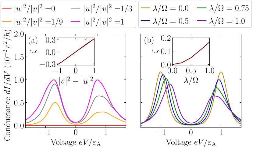
Figure 2: Conductance $dI/dV$ of boson-coupled ABSs vs voltage $V$ calculated using the rate equation [Eq. (5)]. Conductances for (a) different ratios of PH components $|u|^{2}/|v|^{2}$ zsu with $\lambda/\Omega=1$ and (b) different ABS-boson coupling strengths $\lambda$ with $|u|^{2}/|v|^{2}=1/3$. Inset: (a) Conductance PH asymmetry $\zeta$ vs $|v|^{2}-|u|^{2}$ and (b) $\zeta$ vs $\lambda/\Omega$. Due to the ABS-boson coupling $\lambda$, the ABS energy gets renormalized by $\varepsilon_{\mathrm{A}}\rightarrow\varepsilon_{\mathrm{A}}-\lambda^{2}/\Omega$ which shifts the position of the conductance peaks [panel (b)]. The parameters for all panels are: $\varepsilon_{\mathrm{A}}/\Omega=3$, $\Gamma/\Omega=0.05/(2\pi)$, and $k_{\mathrm{B}}T/\Omega=0.4$.

Figure 2 shows the conductance $dI/dV$ (see Sec. V of Ref. sup for the current) of boson-coupled ABSs calculated from Eq. (5). As shown in Fig. 2(a), the conductance decreases with increasing ABS’s PH content imbalance $||u|^{2}-|v|^{2}|$ because the terms $R^{0\rightarrow 1;e}R^{1\rightarrow 0;e}$ and $R^{0\rightarrow 1;h}R^{1\rightarrow 0;h}$ in Eq. (5) are $\propto|uv|^{2}=[1-(|u|^{2}-|v|^{2})^{2}]/4$. In contrast, the conductance PH asymmetry magnitude $|\zeta|$ increases linearly with increasing ABS’s PH content imbalance $||u|^{2}-|v|^{2}|$[inset of Fig. 2(a)], where

$$\zeta\equiv\frac{(dI/dV)_{\mathrm{max},-}-(dI/dV)_{\mathrm{max},+}}{(dI/dV)_{\mathrm{max},-}+(dI/dV)_{\mathrm{max},+}},$$ (6)

with $(dI/dV)_{\mathrm{max},-/+}\equiv\max_{V\leq 0/V\geq 0}dI/dV$ being the peak conductance at negative and positive voltages, respectively. $\zeta=\pm 1$ ($\zeta=0$) corresponds to perfectly asymmetric (symmetric) conductances. Figure 2(b) shows that the peak conductances decrease with increasing ABS-boson coupling strength $\lambda$ since $\lambda$ broadens the quasiparticle weight around the ABS energy, which decreases the effective tunnel coupling strength. The conductance PH asymmetry ($\zeta$) magnitude vsu , however, increases with increasing $\lambda$ [inset of Fig. 2(b)] for $|\tilde{\varepsilon}_{\mathrm{A}}|\gg k_{\mathrm{B}}T$ where the two peaks are well separated. For the regime where $|\tilde{\varepsilon}_{\mathrm{A}}|\approx k_{\mathrm{B}}T$, $\zeta$ has a nonmonotonic behavior with $\lambda$ (see Sec. VI of Ref. sup ). Section VI of Ref. sup shows that $\zeta$ decreases with increasing temperature, depends monotonically on the boson frequency $\Omega$, and prevails only for $\Omega\lesssim 2|\tilde{\varepsilon}_{\mathrm{A}}|+k_{\mathrm{B}}T$.

III.2 Keldysh

For strong-tunneling limit ($\Gamma>k_{\mathrm{B}}T$), we compute the current using the mean-field Keldysh formalism. We begin by rewriting Eq. (2a) in terms of the boson displacement [$\hat{x}=(\hat{b}+\hat{b}^{\dagger})/\sqrt{2}$] and momentum [$\hat{p}=-i(\hat{b}-\hat{b}^{\dagger})/\sqrt{2}$] operator as

$$\hat{H}_{\mathrm{A}} =\varepsilon_{\mathrm{A}}\hat{\gamma}^{\dagger}\hat{\gamma}+\sqrt{2}\lambda\hat{\gamma}^{\dagger}\hat{\gamma}\hat{x}+\frac{\Omega}{2}(\hat{x}^{2}+\hat{p}^{2})-\frac{\Omega}{2}.$$ (7)

We calculate the mean-field energy $\varepsilon_{\mathrm{A}}+\sqrt{2}\lambda\langle\hat{x}\rangle$ by self-consistently solving for $\langle\hat{x}\rangle$ where $\langle\cdots\rangle$ is the expectation value with respect to the mean-field eigenfunction. To this end, we solve for $\partial\langle\hat{H}_{\mathrm{A}}\rangle/\partial\langle\hat{x}\rangle=0$ and $\partial\langle\hat{H}_{\mathrm{A}}\rangle/\partial\langle\hat{p}\rangle=0$, giving $\langle\hat{x}\rangle=-\frac{\sqrt{2}\lambda}{\Omega}\langle\hat{\gamma}^{\dagger}\hat{\gamma}\rangle$ and $\langle\hat{p}\rangle=0$.

The ABS Green’s function in the Lehmann representation is $g_{\mathrm{A}}(\omega)=\frac{\Phi_{+}\Phi^{\dagger}_{+}}{\omega-(\varepsilon_{\mathrm{A}}+\sqrt{2}\lambda\langle\hat{x}\rangle)}+\frac{\Phi_{-}\Phi^{\dagger}_{-}}{\omega+(\varepsilon_{\mathrm{A}}+\sqrt{2}\lambda\langle\hat{x}\rangle)}$ where $\Phi_{+}=(1,0)^{T}$ and $\Phi_{-}=(0,1)^{T}$ are the Nambu spinors written in the Nambu basis $(\hat{\gamma},\hat{\gamma}^{\dagger})^{T}$. Following Ref. Ruby et al. (2015), we use the Green’s function to evaluate the current as (see Sec. VII of Ref. sup )

$$I(V)=\frac{e}{h}\Gamma^{2}\int_{-\infty}^{\infty}d\omega\mathcal{A}(\omega)[f(\omega_{-})-f(\omega_{+})],$$ (8)

where

$$\mathcal{A}(\omega)=\frac{4|uv|^{2}}{\left[\omega-\frac{(\varepsilon_{\mathrm{A}}+\sqrt{2}\lambda\langle\hat{x}\rangle)^{2}}{\omega}-\frac{(\Gamma_{u}-\Gamma_{v})^{2}}{4\omega}\right]^{2}+(\Gamma_{u}+\Gamma_{v})^{2}},$$ (9)

with $\Gamma_{u}=\Gamma|u|^{2}$ and $\Gamma_{v}=\Gamma|v|^{2}$. The mean-field boson displacement $\langle\hat{x}\rangle$ in Eq. (9) is evaluated self-consistently as

$$\langle\hat{x}\rangle =-\frac{\sqrt{2}\lambda}{\Omega}\langle\hat{\gamma}^{\dagger}\hat{\gamma}\rangle=-\frac{\lambda}{\sqrt{2}\Omega}\left\{1-i\int\frac{d\omega}{2\pi}\mathrm{Tr}\left[G^{<}_{\mathrm{A}}(\omega)\sigma_{z}\right]\right\},$$ (10)

where $(G^{<}_{\alpha\beta})_{\mathrm{A}}=i\langle\Psi^{\dagger}_{\alpha\mathrm{A}}\Psi_{\beta\mathrm{A}}\rangle$ is the ABS lesser Green’s function (see Sec. VIII of Ref. sup ) with $\Psi_{\mathrm{A}}=(\hat{\gamma},\hat{\gamma}^{\dagger})^{T}$ and $\sigma_{z}$ being the $z$-Pauli matrix in the Nambu space.

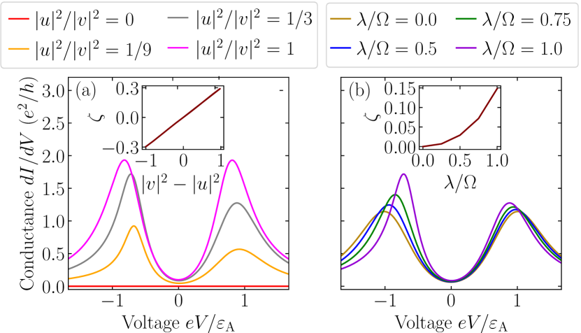
Figure 3: Conductance $dI/dV$ of boson-coupled ABSs vs voltage $V$ calculated using the mean-field Keldysh approach [Eq. (8)]. Conductances for (a) different ratios of PH components $|u|^{2}/|v|^{2}$ zsu with $\lambda/\Omega=1$ and (b) different ABS-boson coupling strengths $\lambda$ with $|u|^{2}/|v|^{2}=1/3$. Inset: (a) Conductance PH asymmetry $\zeta$ vs $|v|^{2}-|u|^{2}$ and (b) $\zeta$ vs $\lambda/\Omega$. Due to the ABS-boson coupling $\lambda$, the ABS energy gets renormalized by $\varepsilon_{\mathrm{A}}\rightarrow\tilde{\varepsilon}_{\mathrm{A}}=\varepsilon_{\mathrm{A}}+\sqrt{2}\lambda\langle\hat{x}\rangle$ (see Sec. V of Ref. sup for the plots of $\langle\hat{x}\rangle$), which shifts the position of the conductance peak [panel (b)]. The parameters for all panels are: $\varepsilon_{\mathrm{A}}/\Omega=3$, $\Gamma/\Omega=2$, and $k_{\mathrm{B}}T/\Omega=0.4$.

Figure 3 shows the conductance (see Sec. V of Ref. sup for the current) of boson-coupled ABSs calculated from Eq. (8) subject to the self-consistency condition [Eq. (10)]. Similar to the rate equation, the conductance of boson-coupled ABSs calculated using the Keldysh approach also decreases with increasing ABS’s PH content imbalance $||u|^{2}-|v|^{2}|$ [Fig. 3(a)] with its PH asymmetry ($\zeta$) magnitude increases linearly with increasing $||u|^{2}-|v|^{2}|$ [inset of Fig. 3(a)]. Figure 3(b) shows that the peak conductance increases with increasing ABS-boson coupling strength $\lambda$ contrary to the rate-equation results. However, similar to the rate-equation, the conductance PH asymmetry $\zeta$ increases with increasing $\lambda$ usu . Unlike the rate equation, the Keldysh approach shows that in the strong-tunneling regime the PHS breaking holds also for high-frequency bosons (see Sec. IX of Ref. sup ), since it arises from nonperturbative effects of tunneling, i.e., the PH asymmetry of the mean-field boson displacement value $\langle\hat{x}\rangle$.

Our model of tunneling into boson-coupled ABS [Eq. (2)] can explain the origin of PH asymmetry for subgap conductance observed in a hard superconducting gap Ménard et al. (2017); Choi et al. (2017); Saldaña et al. (2020); Farinacci et al. (2020); Ding et al. (2021) which cannot be accounted for by QP. However, similar to QP this model also results in conductance peak areas which are independent of temperatures (see Sec. IV B. of Ref. sup ). In Sec. IV below, we consider another related model, i.e., a boson-assisted tunneling model. This model can not only give rise to PHS breaking of subgap conductances but also account for experimentally observed conductance features which cannot be attributed to QP, e.g., an increase in the conductance peak area with temperature Saldaña et al. (2020).

IV Model II. Boson-assisted tunneling into ABS

In this section, we consider boson-assisted tunneling into an ABS via virtual hopping of electrons or holes from the lead into higher-lying states in superconductors which are boson-coupled to the ABS. The higher-lying states can be either higher-energy ABSs or states from the continuum above the gap. By integrating out the higher-lying states, we derive the effective low-energy Hamiltonian for the boson-assisted tunneling into the ABS as (see Sec. X of Ref. sup )

$$\hat{H}_{\mathrm{T}} =t(\hat{b}+\hat{b}^{\dagger})\hat{c}_{\mathrm{L}}^{\dagger}\hat{d}_{\mathrm{A}}+\mathrm{H.c.}$$ (11)

Note the extra $(\hat{b}+\hat{b}^{\dagger})$ term in the above tunneling Hamiltonian as compared to Eq. (2c) in Sec. III.

Figure 4: Current $I$ and conductance $dI/dV$ into ABS vs voltage $V$ for the boson-assisted tunneling model. (Upper panels) Current and (lower panels) conductance for (left panels) different temperatures $k_{\mathrm{B}}T$ with $\lambda/\Omega=0.5$ and (right panels) different ABS-boson coupling strengths $\lambda$ with temperature $k_{\mathrm{B}}T=0.4$. Inset: (a) $I(V=\infty)$ vs $k_{\mathrm{B}}T/\Omega$, (b) Current PH asymmetry $\Xi$ vs $\lambda/\Omega$, (c) Conductance PH asymmetry $\zeta$ vs $k_{\mathrm{B}}T/\Omega$, and (d) $\zeta$ vs $\lambda/\Omega$. Due to the ABS-boson coupling $\lambda$, the ABS energy gets renormalized by $\varepsilon_{\mathrm{A}}\rightarrow\varepsilon_{\mathrm{A}}-\lambda^{2}/\Omega$ which shifts the position of the conductance peaks [panel (d)]. The parameters for all panels are: $|u|=0.1$, $\varepsilon_{\mathrm{A}}/\Omega=6$, and $\Gamma/\Omega=0.05/(2\pi)$.

Figure 4 shows the current and conductance calculated using the rate equation within the boson-assisted tunneling model for different temperatures $T$ and ABS-boson coupling strengths $\lambda$. Contrary to the tunneling model in Sec. III where the current at $V=\pm\infty$ is independent of temperature (see Sec. IV B. of Ref. sup ), for the boson-assisted tunneling model the current magnitude at $V=\pm\infty$ increases with increasing temperature. This is because the boson-assisted tunneling rate (see Sec. X of Ref. sup ) is proportional to $\langle q|(\hat{\tilde{b}}+\hat{\tilde{b}}^{\dagger})^{2}|q\rangle$, which increases with increasing temperature. Crucially, we find that the current $I(V=\pm\infty)$ or equivalently the peak area of the conductance versus voltage curve has a faster-than-linear increase with temperature [inset of Fig. 4(a)], providing excellent agreement with experimental results Saldaña et al. (2020). Since QP preserves the conductance peak area under different temperatures and necessarily induces “soft-gap” conductance features, our proposed boson-assisted tunneling process is thus more likely to be responsible for the PH-asymmetric subgap conductances inside a hard superconducting gap observed in Ref. Saldaña et al. (2020).

Contrary to the model in Sec. III, for the boson-assisted tunneling model, the current calculated at large positive and negative voltages need not be perfectly antisymmetric, i.e., $I(V=\infty)\neq-I(V=-\infty)$. The current PH asymmetry $\Xi$, defined as

$$\Xi\equiv\frac{|I(V=-\infty)|-|I(V=\infty)|}{|I(V=-\infty)|+|I(V=\infty)|},$$ (12)

increases with increasing ABS-boson coupling strength $\lambda$ [see inset of Fig. 4(b)]. This current PH asymmetry (or equivalently the asymmetry between the conductance peak area for positive and negative voltages) as well as the dependence of the conductance peak area with temperature can serve as signatures for the boson-assisted tunneling process. Similar to the model in Sec. III, the conductance PH asymmetry $\zeta$ calculated using the boson-assisted tunneling model also decreases with increasing temperature [inset of Fig. 4(c)] and increases with increasing ABS-boson coupling strength $\lambda$ [inset of Fig. 4(d)].

V Conclusions

Contrary to widely held belief, we show that the PHS breaking of subgap conductances in superconductors can arise without QP. Specifically, the coupling of ABSs to a bosonic bath (or multimode bosonic baths mul ) can break the PHS of subgap conductances without changing the superconductor’s parity state. Therefore, contrary to QP, our mechanism is not detrimental to the coherence of superconductor-based qubits. (Topological qubits are exponentially protected from the bosonic bath dephasing due to the spatial separation of Majoranas Knapp et al. (2018).) We find that the conductance PH asymmetry increases with increasing ABS’s PH content imbalance, increasing ABS-boson coupling strength and decreasing temperature. Our theory is general as it applies to all ABSs, e.g., quasi-Majorana states Kells et al. (2012); Liu et al. (2017b), Yu-Shiba-Rusinov states Yu (1965); Shiba (1968); Rusinov (1969), Caroli-de Gennes-Matricon states Caroli et al. (1964), etc., which couple to bosonic modes such as phonons, plasmons, electromagnetic fields, etc., in superconductors. Contrary to QP, our mechanism applies even for ABSs observed inside a hard superconducting gap Ménard et al. (2017); Choi et al. (2017); Saldaña et al. (2020); Ding et al. (2021) and can give rise to an increase in the conductance peak area with temperature as observed in experiments Saldaña et al. (2020).

Our PHS breaking mechanism results from boson emissions or absorptions accompanying the electron/hole tunneling. Since these bosons such as phonons are ubiquitous in superconductors, we expect electron-phonon interactions (EPIs) to significantly affect transport in superconductors, particularly the semiconductor-superconductor heterostructures used to realize topological superconductors Suominen et al. (2017); Nichele et al. (2017); Ménard et al. (2017); Gül et al. (2018); Deng et al. (2018); Bommer et al. (2019); Chen et al. (2019); Vaitiekėnas et al. (2020); Yu et al. (2021). In fact, measurements of transport in semiconductors have observed features Huntzinger et al. (2000); Goldman et al. (1987); Hartke et al. (2018); Roulleau et al. (2011); Weber et al. (2010) associated with EPI that are theoretically understood Muljarov and Zimmermann (2004); Kleinman (1965); Wingreen et al. (1988). We estimate that for a typical topological superconductor which uses either an InAs or InSb semiconductor with a length of $\ell\sim 1$ $\mu$m (having a phonon frequency $\Omega\sim\hbar v_{s}\pi/\ell=7.2$ $\mu$eV where $v_{s}\approx 3.5\times 10^{5}$ cm/s Yano et al. (1993); Wagner et al. (1995); Madelung (2012) is the sound velocity), EPI can give rise to a conductance PH asymmetry in the tunneling limit for ABSs with energies $\varepsilon_{\mathrm{A}}\gtrsim\Omega/2=3.6$ $\mu$eV. Therefore, contrary to QP, EPI does not affect the zero-bias Majorana conductance.

Compared to diagrammatic techniques, FGR is a more controlled approach in treating the effect of interactions on transport in superconductors (even for strongly correlated superconductors) for the strict tunneling limit. This is because interaction diagrams can generate an imaginary self-energy Ruby et al. (2015), resulting in a conductance PH asymmetry similar to QP Martin and Mozyrsky (2014). Therefore, it is crucial to enforce a fermion parity conservation in the diagrammatic treatment of ABS-boson couplings like our mean-field treatment of interactions in the Keldysh formulation. Our work thus motivates the formulation of the nonequilibrium Green’s function beyond the mean field approximation that conserves fermion parity. We note that our mechanism is quite distinct from the subgap-conductance PHS breaking due to the bias-voltage dependence of the tunnel barrier Melo et al. (2021). While this mechanism can be treated within the Keldysh approach by moving the interaction term from the ABS to the barrier, it vanishes in the tunneling limit where FGR applies.

Supplemental Material for “Electron-boson-interaction induced particle-hole symmetry breaking of conductance into subgap states in superconductors”

I Derivation of the ABS-boson coupling from the microscopic electron-boson interaction

In this section, we derive the ABS-boson coupling term in Eq. (2a) of the main text from the microscopic electron-boson interaction. We begin by writing a generic Hamiltonian for a superconductor with an ABS as

$$\hat{H}_{\mathrm{SC}}=\sum_{l,m}\int dx\int dx^{\prime}h_{lm}(x,x^{\prime})\hat{d}_{l}^{\dagger}(x)\hat{d}_{m}(x^{\prime})+\left[\Delta_{lm}(x,x^{\prime})\hat{d}_{l}^{\dagger}(x)\hat{d}^{\dagger}_{m}(x^{\prime})+\mathrm{H.c.}\right],$$ (S-1)

where $h_{l,m}$ describes the dynamics of the electrons in the superconductor with an ABS, $\Delta_{l,m}$ is the superconducting pairing potential, $d_{l,m}^{\dagger}$ ($d_{l,m}$) is the electron creation (annihilation) operator of the superconductor and the indices $l,m$ represent both the orbital and spin degrees of freedom. We can diagonalize the above Hamiltonian using the Bogoliubov transformation

$$\hat{\gamma}_{\alpha} =\sum_{m}\int dx\left[u_{\alpha m}^{*}(x)d_{m}(x)+v_{\alpha m}(x)d_{m}^{\dagger}(x)\right],$$ (S-2a)

$$\hat{\gamma}_{\alpha}^{\dagger} =\sum_{m}\int dx\left[v_{\alpha m}^{*}(x)d_{m}(x)+u_{\alpha m}(x)d_{m}^{\dagger}(x)\right],$$ (S-2b)

which gives

$$\hat{H}_{\mathrm{SC}}=\sum_{\alpha}\varepsilon_{\alpha}\hat{\gamma}_{\alpha}^{\dagger}\hat{\gamma}_{\alpha}+\mathrm{const},$$ (S-3)

where the lowest energy level corresponds to the ABS energy, i.e., $\varepsilon_{1}=\varepsilon_{\mathrm{A}}$.

The Hamiltonian of the electron-boson coupling is given by

$$\hat{H}_{\text{e-b}}=\sum_{lm}\int dx\int dx^{\prime}g_{lm}(x,x^{\prime})\hat{d}^{\dagger}_{l}(x)\hat{d}_{m}(x^{\prime})(\hat{b}^{\dagger}+\hat{b}),$$ (S-4)

where $g_{lm}$ is the electron-boson coupling strength, and $\hat{b}$ ($\hat{b}^{\dagger}$) is the boson annihilation (creation) operator. Substituting

$$d_{m}(x) =\sum_{\alpha>0}\left[u_{m\alpha}(x)\hat{\gamma}_{\alpha}+v_{m\alpha}(x)\hat{\gamma}_{\alpha}^{\dagger}\right],$$ (S-5a)

$$d_{m}^{\dagger}(x) =\sum_{\alpha>0}\left[v_{m\alpha}^{*}(x)\hat{\gamma}_{\alpha}+u_{m\alpha}^{*}(x)\hat{\gamma}_{\alpha}^{\dagger}\right],$$ (S-5b)

into Eq. (S-4), we have

$$\hat{H}_{\text{e-b}} =\sum_{lm\alpha\beta}\int dx\int dx^{\prime}g_{lm}(x,x^{\prime})\left[v_{l\alpha}^{*}(x)u_{m\beta}(x^{\prime})\hat{\gamma}_{\alpha}\hat{\gamma}_{\beta}+v_{l\alpha}^{*}(x)v_{m\beta}(x^{\prime})\hat{\gamma}_{\alpha}\hat{\gamma}^{\dagger}_{\beta}\right.$$

$$\hskip 156.49014pt\left.+u_{l\alpha}^{*}(x)u_{m\beta}(x^{\prime})\hat{\gamma}_{\alpha}^{\dagger}\hat{\gamma}_{\beta}+u^{*}_{l\alpha}(x)v_{m\beta}(x^{\prime})\hat{\gamma}_{\alpha}^{\dagger}\hat{\gamma}_{\beta}^{\dagger}\right](\hat{b}^{\dagger}+\hat{b})$$

$$=\sum_{\alpha,\beta}\biggl{(}\tilde{\lambda}^{(c)}_{\alpha\beta}\gamma^{\dagger}_{\alpha}\gamma_{\beta}+\tilde{\lambda}^{(d)}_{\alpha\beta}\gamma_{\alpha}\gamma_{\beta}\biggr{)}(\hat{b}^{\dagger}+\hat{b})+\mathrm{H.c.},$$ (S-6)

where we have defined

$$\tilde{\lambda}^{(c)}_{\alpha\beta} \equiv\frac{1}{2}\sum_{lm}\int dx\int dx^{\prime}g_{lm}(x,x^{\prime})[u_{l\alpha}^{*}(x)u_{m\beta}(x^{\prime})-v_{l\beta}^{*}(x)v_{m\alpha}(x^{\prime})],$$

$$\tilde{\lambda}^{(d)}_{\alpha\beta} \equiv\sum_{lm}\int dx\int dx^{\prime}g_{lm}(x,x^{\prime})[v_{l\alpha}^{*}(x)u_{m\beta}(x^{\prime})].$$ (S-7)

Projecting the above Hamiltonian into the lowest energy sector $\alpha=\beta=1$ which corresponds to the ABS energy sector, we have

$$\hat{H}_{\text{e-b}} \approx\sum_{lm}\int dx\int dx^{\prime}g_{lm}(x,x^{\prime})[u_{l1}^{*}(x)u_{m1}(x^{\prime})-v_{l1}^{*}(x)v_{m1}(x^{\prime})]\hat{\gamma}^{\dagger}\hat{\gamma}(\hat{b}^{\dagger}+\hat{b})+\sum_{lm}\int dx\int dx^{\prime}g_{lm}(x,x^{\prime})(\hat{b}^{\dagger}+\hat{b})$$

$$=\lambda\hat{\gamma}^{\dagger}\hat{\gamma}(\hat{b}^{\dagger}+\hat{b})+\chi(\hat{b}^{\dagger}+\hat{b}),$$ (S-8)

where we have defined $\hat{\gamma}\equiv\hat{\gamma}_{1}$ as the Bogoliubov operator for the ABS, $\lambda\equiv 2\lambda_{11}^{(c)}$ as the ABS-boson coupling strength, and $\chi\equiv\sum_{lm}\int dx\int dx^{\prime}g_{lm}(x,x^{\prime})$. Note that in evaluating Eq. (I), we have used the anticommutation relation $\{\gamma,\gamma^{\dagger}\}=1$, $\{\gamma,\gamma\}=0$, and $\{\gamma^{\dagger},\gamma^{\dagger}\}=0$. We can eliminate the term $\chi(\hat{b}^{\dagger}+\hat{b})$ in Eq. (I) by introducing the shift $\hat{b}\rightarrow\hat{b}-\chi/\Omega$ and $\hat{b}^{\dagger}\rightarrow\hat{b}^{\dagger}-\chi/\Omega$ which gives the ABS Hamiltonian as

$$\hat{H}_{\mathrm{A}} =\varepsilon_{\mathrm{A}}\gamma^{\dagger}\gamma+\lambda\hat{\gamma}^{\dagger}\hat{\gamma}\left(\hat{b}+\hat{b}^{\dagger}-2\frac{\chi}{\Omega}\right)+\chi\left(\hat{b}^{\dagger}+\hat{b}-2\frac{\chi}{\Omega}\right)+\Omega\left(\hat{b}^{\dagger}-\frac{\chi}{\Omega}\right)\left(\hat{b}-\frac{\chi}{\Omega}\right)$$

$$=\left(\varepsilon_{\mathrm{A}}-2\frac{\lambda\chi}{\Omega}\right)\gamma^{\dagger}\gamma+\lambda\hat{\gamma}^{\dagger}\hat{\gamma}\left(\hat{b}^{\dagger}+\hat{b}\right)+\Omega\hat{b}^{\dagger}\hat{b}-\frac{\chi^{2}}{\Omega}.$$ (S-9)

Introducing the shift $\varepsilon_{\mathrm{A}}\rightarrow\varepsilon_{\mathrm{A}}+2\lambda\chi/\Omega$ and shifting the overall energy by $\frac{\chi^{2}}{\Omega}$, i.e., $\hat{H}_{\mathrm{A}}\rightarrow\hat{H}_{\mathrm{A}}-\frac{\chi^{2}}{\Omega}$, we have the Hamiltonian for the boson-coupled ABS as in Eq. (2a) of the main text:

$$\hat{H}_{\mathrm{A}} =\varepsilon_{\mathrm{A}}\hat{\gamma}^{\dagger}\hat{\gamma}+\lambda\hat{\gamma}^{\dagger}\hat{\gamma}(\hat{b}^{\dagger}+\hat{b})+\Omega\hat{b}^{\dagger}\hat{b}.$$ (S-10)

II Lang-Firsov Transformation

In this section, we follow Ref. Mahan (2000) to derive the matrix elements for the tunneling of electrons ($\hat{d}_{\mathrm{A}}^{\dagger}$) and holes ($\hat{d}_{\mathrm{A}}$) and the boson absorption or emission matrix elements $Y_{qq^{\prime}}$ in Eq. (III.1) of the main text. We begin by writing the Hamiltonian of an ABS coupled to a one-dimensional normal lead and bosonic modes, e.g., phonons, plasmons, etc., as the sum of the Hamiltonian of a boson-coupled ABS, lead and tunnel coupling, $\hat{H}=\hat{H}_{\mathrm{A}}+\hat{H}_{\mathrm{L}}+\hat{H}_{\mathrm{T}}$ [Eq. (2) of the main text], where

$$\hat{H}_{\mathrm{A}} =\varepsilon_{\mathrm{A}}\hat{\gamma}^{\dagger}\hat{\gamma}+\lambda\hat{\gamma}^{\dagger}\hat{\gamma}(\hat{b}^{\dagger}+\hat{b})+\Omega\hat{b}^{\dagger}\hat{b},$$ (S-11a)

$$\hat{H}_{\mathrm{L}} =\sum_{k}\varepsilon_{\mathrm{L},k}\hat{c}_{\mathrm{L},k}^{\dagger}\hat{c}_{\mathrm{L},k},$$ (S-11b)

$$\hat{H}_{\mathrm{T}} =t\hat{c}_{\mathrm{L}}^{\dagger}\hat{d}_{\mathrm{A}}+\mathrm{H.c.}$$ (S-11c)

Here, $\varepsilon_{\mathrm{A}}$ is the ABS energy, $\hat{\gamma}$ ($\hat{\gamma}^{\dagger}$) is the Bogoliubov annihilation (creation) operator of the ABS, $\lambda$ is the ABS-boson coupling strength, $\hat{b}$ ($\hat{b}^{\dagger}$) is the boson annihilation (creation) operator and $\Omega$ is the boson frequency. The operator $\hat{c}_{\mathrm{L},k}$ ($\hat{c}_{\mathrm{L},k}^{\dagger}$) annihilates (creates) the lead electron with momentum $k$ and energy $\varepsilon_{\mathrm{L},k}$. The tunneling Hamiltonian $H_{T}$ Balatsky et al. (2006); Ruby et al. (2015) represents the electron tunneling between the normal lead and ABS, where the electron annihilation operator of the lead and ABS at the junction given by $\hat{c}_{\mathrm{L}}=\int dk\hat{c}_{\mathrm{L},k}/(2\pi)$ and $\hat{d}_{\mathrm{A}}$, respectively. The operator $\hat{d}_{\mathrm{A}}$ is obtained by projecting the operator $\hat{d}_{1}(x=0)$ [Eq. (S-5a)] to the ABS energy sector ($\alpha=1$), where we have $\hat{d}_{\mathrm{A}}=u\gamma+v\gamma^{\dagger}$. For notational simplicity, here we define $\gamma\equiv\gamma_{1}$, $u\equiv u_{\mathrm{11}}(x=0)$ and $v\equiv v_{\mathrm{11}}(x=0)$ where $u$ and $v$ are the particle and hole components of the ABS wave function at the junction ($x=0$). In this paper, we renormalize the ABS wave function such that $|u|^{2}+|v|^{2}=1$. Note that since we consider only the subgap state and ignore the above-gap states, the relation $\hat{d}_{\mathrm{A}}=u\gamma+v\gamma^{\dagger}$ is only approximate which makes $\hat{d}_{\mathrm{A}}$ nonfermionic. The operator $\hat{d}_{\mathrm{A}}$ becomes fermionic if all the states in the superconductor including the above-gap states are taken into account [see Eq. (S-5a)]. Our conclusion on the PHS breaking of the subgap conductance due to the ABS-boson coupling does not rely on the fermionic properties of $\hat{d}_{\mathrm{A}}$.

To eliminate the ABS-boson coupling, we can transform the Hamiltonian [Eq. (S-11)] using a canonical transformation

$$\hat{\tilde{H}}=e^{\hat{S}}\hat{H}e^{-\hat{S}},$$ (S-12)

where

$$\hat{S} =\frac{\lambda}{\Omega}\hat{\gamma}^{\dagger}\hat{\gamma}(\hat{b}^{\dagger}-\hat{b})$$ (S-13)

is the Lang-Firsov transformation operator Lang and Firsov (1963). Using the relation

$$\hat{\tilde{A}} =e^{\hat{S}}\hat{A}e^{-\hat{S}}=\hat{A}+[\hat{S},\hat{A}]+\frac{1}{2!}[\hat{S},[\hat{S},\hat{A}]]+\cdots,$$ (S-14)

we can write the transformed annihilation and creation operators for the Bogoliubov quasiparticles, electrons and bosonic modes as

$$\hat{\tilde{\gamma}} =\hat{\gamma}\hat{Y},$$ (S-15a)

$$\hat{\tilde{\gamma}}^{\dagger} =\hat{\gamma}^{\dagger}\hat{Y}^{\dagger},$$ (S-15b)

$$\hat{\tilde{d}}_{\mathrm{A}} =u\hat{\gamma}\hat{Y}+v\hat{\gamma}^{\dagger}\hat{Y}^{\dagger},$$ (S-15c)

$$\hat{\tilde{d}}_{\mathrm{A}}^{\dagger} =u^{*}\hat{\gamma}^{\dagger}\hat{Y}^{\dagger}+v^{*}\hat{\gamma}\hat{Y},$$ (S-15d)

$$\hat{\tilde{b}} =\hat{b}-\frac{\lambda}{\Omega}\hat{\gamma}^{\dagger}\hat{\gamma},$$ (S-15e)

$$\hat{\tilde{b}}^{\dagger} =\hat{b}^{\dagger}-\frac{\lambda}{\Omega}\hat{\gamma}^{\dagger}\hat{\gamma},$$ (S-15f)

where $\hat{Y}=\mathrm{exp}\left[-\frac{\lambda}{\Omega}(\hat{b}^{\dagger}-\hat{b})\right]$. Under this transformation, the number operator remains the same, i.e., $\hat{\tilde{\gamma}}^{\dagger}\hat{\tilde{\gamma}}=\hat{\gamma}^{\dagger}\hat{\gamma}\hat{Y}^{\dagger}\hat{Y}=\hat{\gamma}^{\dagger}\hat{\gamma}$ and the Hamiltonians [Eq. (S-11a) and Eq. (S-11c)] transform as

$$\hat{\tilde{H}}_{\mathrm{A}} =\varepsilon_{\mathrm{A}}\hat{\gamma}^{\dagger}\hat{\gamma}+\lambda\left(\hat{b}^{\dagger}+\hat{b}-\frac{2\lambda}{\Omega}\hat{\gamma}^{\dagger}\hat{\gamma}\right)\hat{\gamma}^{\dagger}\hat{\gamma}+\Omega\left(\hat{b}^{\dagger}-\frac{\lambda}{\Omega}\hat{\gamma}^{\dagger}\hat{\gamma}\right)\left(\hat{b}-\frac{\lambda}{\Omega}\hat{\gamma}^{\dagger}\hat{\gamma}\right)$$ (S-16a)

$$=\left(\varepsilon_{\mathrm{A}}-\frac{\lambda^{2}}{\Omega}\right)\hat{\gamma}^{\dagger}\hat{\gamma}+\Omega\hat{b}^{\dagger}\hat{b},$$

$$\hat{\tilde{H}}_{\mathrm{T}} =t\hat{c}_{\mathrm{L}}^{\dagger}\hat{\tilde{d}}_{\mathrm{A}}+\mathrm{H.c.},$$ (S-16b)

where $\hat{\tilde{d}}_{\mathrm{A}}=u\hat{\gamma}\hat{Y}+v\hat{\gamma}^{\dagger}\hat{Y}^{\dagger}$ is the Lang-Firsov transformation of $\hat{d}_{\mathrm{A}}$.

We can evaluate the matrix elements for the electron and hole tunneling which change the ABS occupancy number $n$ from $0\rightarrow 1$ and the boson occupancy from $q\rightarrow q^{\prime}$ as

$$\langle 1,q^{\prime}|\hat{\tilde{d}}_{\mathrm{A}}^{\dagger}|0,q\rangle =u^{*}\langle 1|\hat{\gamma}^{\dagger}|0\rangle\langle q^{\prime}|\hat{Y}^{\dagger}|q\rangle=u^{*}Y_{qq^{\prime}},$$ (S-17a)

$$\langle 1,q^{\prime}|\hat{\tilde{d}}_{\mathrm{A}}|0,q\rangle =v\langle 1|\hat{\gamma}^{\dagger}|0\rangle\langle q^{\prime}|\hat{Y}^{\dagger}|q\rangle=vY_{qq^{\prime}},$$ (S-17b)

respectively. Using the Baker-Campbell-Haussdorf formula, we have

$$\hat{Y}^{\dagger}=e^{\frac{\lambda}{\Omega}(\hat{b}^{\dagger}-\hat{b})}=e^{-\frac{\lambda^{2}}{2\Omega^{2}}}e^{\frac{\lambda}{\Omega}\hat{b}^{\dagger}}e^{-\frac{\lambda}{\Omega}\hat{b}},$$ (S-18)

and we can evaluate the boson emission or absorption matrix element as Mitra et al. (2004)

$$Y_{qq^{\prime}}\equiv\langle q^{\prime}|\hat{Y}^{\dagger}|q\rangle=\langle q^{\prime}|e^{\frac{\lambda}{\Omega}(b^{\dagger}-b)}|q\rangle =\langle q^{\prime}|e^{-\frac{\lambda^{2}}{2\Omega^{2}}}e^{\frac{\lambda}{\Omega}\hat{b}^{\dagger}}e^{-\frac{\lambda}{\Omega}\hat{b}}|q\rangle$$

$$=e^{-\frac{\lambda^{2}}{2\Omega^{2}}}\sum_{m=0}^{\mathrm{min}(q,q^{\prime})}\left(\frac{\lambda}{\Omega}\right)^{q^{\prime}-m}\left(-\frac{\lambda}{\Omega}\right)^{q-m}\frac{\sqrt{q!q^{\prime}!}}{m!(q-m)!(q^{\prime}-m)!},$$ (S-19)

where $|Y_{qq^{\prime}}|^{2}$ is symmetric under the interchange $q\leftrightarrow q^{\prime}$. Note that in going to the second line of Eq. (II), we have used the following relations:

$$e^{-\frac{\lambda}{\Omega}\hat{b}}|q\rangle =\sum_{m=0}^{\infty}\frac{1}{m!}\left(-\frac{\lambda}{\Omega}\right)^{m}\hat{b}^{m}|q\rangle=\sum_{m=0}^{q}\frac{1}{m!}\left(-\frac{\lambda}{\Omega}\right)^{m}\sqrt{\frac{q!}{(q-m)!}}|q-m\rangle,$$ (S-20a)

$$\langle q^{\prime}|e^{\frac{\lambda}{\Omega}\hat{b}^{\dagger}} =\sum_{l=0}^{\infty}\frac{1}{l!}\left(\frac{\lambda}{\Omega}\right)^{l}\langle q^{\prime}|(\hat{b}^{\dagger})^{l}=\sum_{l=0}^{q^{\prime}}\frac{1}{l!}\left(\frac{\lambda}{\Omega}\right)^{l}\sqrt{\frac{q^{\prime}!}{(q^{\prime}-l)!}}\langle q^{\prime}-l|.$$ (S-20b)

III Rate equation and tunneling rates

The stationary-state rate equation satisfied by the probability $P_{q}^{n}$ of an ABS-boson system being in the state $|n,q\rangle$, i.e., having an ABS occupation number $n$ and boson occupation number $q$, is given by Mitra et al. (2004); Koch et al. (2004)

$$0 =\frac{\partial P_{q}^{n}}{\partial t}$$

$$=\sum_{q^{\prime}}P_{q^{\prime}}^{\bar{n}}\left[R^{\bar{n}\rightarrow n;e}_{q^{\prime}\rightarrow q}+R^{\bar{n}\rightarrow n;h}_{q^{\prime}\rightarrow q}\right]-P_{q}^{n}\sum_{q^{\prime}}\left[R^{n\rightarrow\bar{n};e}_{q\rightarrow q^{\prime}}+R^{n\rightarrow\bar{n};h}_{q\rightarrow q^{\prime}}\right]$$

$$\hskip 28.45274pt+P^{n}_{q+1}\eta_{q+1;-}+P^{n}_{q-1}\eta_{q-1;+}-P_{q}^{n}\left(\eta_{q;+}+\eta_{q;-}\right).$$ (S-21)

The second line in Eq. (III) represents the probability flux due to hopping of an electron ($e$) or hole ($h$) from the lead to the ABS which changes the ABS occupation number from $\bar{n}\equiv 1-n$ to $n$ and the boson occupancy from $q^{\prime}$ to $q$ and vice versa. The quantity $P_{q}^{n}$ denotes the probability that the system is in the state $|n,q\rangle$ and $R_{q\rightarrow q^{\prime}}^{n\rightarrow\bar{n}}$ denotes the transition rate from the state $|n,q\rangle$ to the state $|\bar{n},q^{\prime}\rangle$. The third line of Eq. (III) represents the boson relaxation where the boson emission and absorption probabilities are $\eta_{q;+}=A(q+1)$ and $\eta_{q;-}=Bq$, respectively, with $A=Be^{-\Omega/k_{\mathrm{B}}T}$. These probability rates are consistent with the fluctuation-dissipation theorem. If the boson relaxation rate is faster than the tunneling rate $\Gamma/\hbar$ such that the bosons acquire the equilibrium distribution $P^{\mathrm{b}}_{q}=e^{-q\Omega/k_{\mathrm{B}}T}(1-e^{-\Omega/k_{\mathrm{B}}T})$, the probability $P_{q}^{n}$ can be factorized as $P_{q}^{n}=P^{n}P^{\mathrm{b}}_{q}$. Summing Eq. (III) over $q$ for these factorized probabilities gives

$$0=P^{\bar{n}}(R^{\bar{n}\rightarrow n;e}+R^{\bar{n}\rightarrow n;h})-P^{n}\left(R^{n\rightarrow\bar{n};e}+R^{n\rightarrow\bar{n};h}\right)+P^{n}\sum_{q}\left[P^{\mathrm{b}}_{q+1}\eta_{q+1;-}+P^{\mathrm{b}}_{q-1}\eta_{q-1;+}-P^{\mathrm{b}}_{q}\left(\eta_{q;+}+\eta_{q;-}\right)\right],$$ (S-22)

where $R^{n\rightarrow\bar{n};e(h)}\equiv\sum_{q,q^{\prime}}P^{\mathrm{b}}_{q}R^{n\rightarrow\bar{n};e(h)}_{q\rightarrow q^{\prime}}$ and $R^{\bar{n}\rightarrow n;e(h)}\equiv\sum_{q,q^{\prime}}P^{\mathrm{b}}_{q^{\prime}}R^{\bar{n}\rightarrow n;e(h)}_{q^{\prime}\rightarrow q}$. Since the sum of the boson relaxation terms over $q$ [the last four terms in Eq. (S-22)] is zero, Eq. (S-22) then reduces to Eq. (3) of the main text.

For the tunneling Hamiltonian in Eq. (S-16b), the rates of the electron and hole tunneling processes can be calculated from Fermi’s Golden Rule to be

$$R^{n\rightarrow\bar{n};e}_{q\rightarrow q^{\prime}} =\frac{2\pi t^{2}\nu_{0}}{\hbar}\left|\left\langle\bar{n},q^{\prime}\left|\hat{\tilde{d}}_{\mathrm{A}}^{\dagger}\right|n,q\right\rangle\right|^{2}f(E_{\bar{n},q^{\prime}}-E_{n,q}-eV)$$

$$=\frac{\Gamma}{\hbar}|\langle\bar{n}|\hat{d}_{\mathrm{A}}^{\dagger}|n\rangle|^{2}|Y_{qq^{\prime}}|^{2}f(E_{\bar{n},q^{\prime}}-E_{n,q}-eV),$$ (S-23a)

$$R^{n\rightarrow\bar{n};h}_{q\rightarrow q^{\prime}} =\frac{2\pi t^{2}\nu_{0}}{\hbar}\left|\left\langle\bar{n},q^{\prime}\left|\hat{\tilde{d}}_{\mathrm{A}}\right|n,q\right\rangle\right|^{2}f(E_{\bar{n},q^{\prime}}-E_{n,q}+eV)$$

$$=\frac{\Gamma}{\hbar}|\langle\bar{n}|\hat{d}_{\mathrm{A}}|n\rangle|^{2}|Y_{qq^{\prime}}|^{2}f(E_{\bar{n},q^{\prime}}-E_{n,q}+eV),$$ (S-23b)

where $\langle\bar{n}|\hat{d}_{\mathrm{A}}^{\dagger}|n\rangle$ and $\langle\bar{n}|\hat{d}_{\mathrm{A}}|n\rangle$ are the bare tunneling matrix elements for electrons and holes, respectively, $Y_{qq^{\prime}}=\langle q^{\prime}|e^{-\lambda(\hat{b}^{\dagger}-\hat{b})/\Omega}|q\rangle$ is the boson emission or absorption matrix element, and $f(E)=[1+\mathrm{exp}({E/k_{\mathrm{B}}T})]^{-1}$ is the lead Fermi function.

IV Details on Model I. Tunneling into Boson-Coupled ABS

IV.1 Proof for the particle-hole asymmetry of boson-coupled-ABS conductance

In this section, we will prove that, unless $|u|=|v|$, the current into a boson-coupled ABS [Eq. (5) of the main text] is in general not PH antisymmetric, i.e., $I(V_{0})\neq I(-V_{0})$ resulting in a PH asymmetric conductance, i.e., $\left.\frac{dI}{dV}\right|_{V=V_{0}}\neq\left.\frac{dI}{dV}\right|_{V=-V_{0}}$. Substituting the transition rates

$$R^{0\rightarrow 1;e} =\Gamma|u|^{2}W(\tilde{\varepsilon}_{\mathrm{A},-})/\hbar,$$ (S-24a)

$$R^{1\rightarrow 0;e} =\Gamma|v|^{2}W(-\tilde{\varepsilon}_{\mathrm{A},+})/\hbar,$$ (S-24b)

$$R^{0\rightarrow 1;h} =\Gamma|v|^{2}W(\tilde{\varepsilon}_{\mathrm{A},+})/\hbar,$$ (S-24c)

$$R^{1\rightarrow 0;h} =\Gamma|u|^{2}W(-\tilde{\varepsilon}_{\mathrm{A},-})/\hbar,$$ (S-24d)

into Eq. (III.1) of the main text, we can evaluate the current [Eq. (5) of the main text] as

$$I =\frac{2e}{\hbar}\frac{\Gamma|uv|^{2}\left[W(\tilde{\varepsilon}_{\mathrm{A},-})W(-\tilde{\varepsilon}_{\mathrm{A},+})-W(\tilde{\varepsilon}_{\mathrm{A},+})W(-\tilde{\varepsilon}_{\mathrm{A},-})\right]}{|u|^{2}F(\tilde{\varepsilon}_{\mathrm{A},-})+|v|^{2}F(\tilde{\varepsilon}_{\mathrm{A},+})},$$ (S-25)

where

$$W(x) =\sum_{q,q^{\prime}}P^{\mathrm{b}}_{q}|Y_{qq^{\prime}}|^{2}f(x-\Omega(q-q^{\prime})),$$ (S-26a)

$$\tilde{\varepsilon}_{\mathrm{A},\pm} =\varepsilon_{\mathrm{A}}-\lambda^{2}/\Omega\pm eV,$$ (S-26b)

$$F(x) =W(x)+W(-x),$$ (S-26c)

with $f(x)=[1+\mathrm{exp}({x/k_{\mathrm{B}}T})]^{-1}$ being the Fermi function.

We will prove below that the function $F(x)$ in the denominator of Eq. (S-25) is an increasing function of $x$ and hence the denominator in Eq. (S-25) is asymmetric with respect to the interchange $V\leftrightarrow-V$ unless $|u|=|v|$. By rewriting $W(x)$ in Eq. (S-26a) as

$$W(x) =\int_{-\infty}^{\infty}d\omega Q(\omega)f(x-\omega),$$ (S-27)

where

$$Q(\omega)=\sum_{q,q^{\prime}}P^{\mathrm{b}}_{q}|Y_{qq^{\prime}}|^{2}\delta(\omega-\Omega(q-q^{\prime})),$$ (S-28)

we have

$$F(x)\equiv W(x)+W(-x) =\int_{-\infty}^{\infty}[Q(\omega)-Q(-\omega)]f(x-\omega)d\omega+\sum_{q,q^{\prime}}P^{\mathrm{b}}_{q}|Y_{qq^{\prime}}|^{2}$$

$$=\int_{0}^{\infty}[Q(\omega)-Q(-\omega)][f(x-\omega)-f(x+\omega)]d\omega+\sum_{q,q^{\prime}}P^{\mathrm{b}}_{q}|Y_{qq^{\prime}}|^{2}$$

$$=\frac{1}{2}\int_{0}^{\infty}\left[Q(\omega)-Q(-\omega)\right]\left[\mathrm{tanh}\left(\frac{x+\omega}{2k_{\mathrm{B}}T}\right)-\mathrm{tanh}\left(\frac{x-\omega}{2k_{\mathrm{B}}T}\right)\right]d\omega+\sum_{q,q^{\prime}}P^{\mathrm{b}}_{q}|Y_{qq^{\prime}}|^{2}.$$ (S-29)

In the following, we will prove that $F(x)$ is a monotonic function of $x$. We first begin by noting that $Q(\omega)-Q(-\omega)\leq 0$ for $\omega\geq 0$. The proof is as follows

$$Q(\omega)-Q(-\omega) =\sum_{q,q^{\prime}}P^{\mathrm{b}}_{q}|Y_{qq^{\prime}}|^{2}\left[\delta(\omega-\Omega(q-q^{\prime}))-\delta(-\omega-\Omega(q-q^{\prime}))\right]$$

$$=\sum_{q,q^{\prime}}P^{\mathrm{b}}_{q}|Y_{qq^{\prime}}|^{2}\left[\delta(\omega-\Omega(q-q^{\prime}))-\delta(\omega+\Omega(q-q^{\prime}))\right]$$

$$=\sum_{q,q^{\prime}}(P^{\mathrm{b}}_{q}-P^{\mathrm{b}}_{q^{\prime}})|Y_{qq^{\prime}}|^{2}\delta(\omega-\Omega(q-q^{\prime})),$$ (S-30)

where in the third line we interchange $q$ with $q^{\prime}$ for the second sum and use $|Y_{qq^{\prime}}|^{2}=|Y_{q^{\prime}q}|^{2}$. For $\omega\geq 0$, the delta function forces $q\geq q^{\prime}$ implying that $(P^{\mathrm{b}}_{q}-P^{\mathrm{b}}_{q^{\prime}})\propto\mathrm{exp}(-q\Omega/k_{\mathrm{B}}T)-\mathrm{exp}(-q^{\prime}\Omega/k_{\mathrm{B}}T)\leq 0$. As a result, $Q(\omega)-Q(-\omega)\leq 0$.

To prove that $F(x)$ is a monotonic function of $x$, we take the derivative of $F(x)$ [Eq. (IV.1)] with $x$ which gives

$$F^{\prime}(x)=\frac{1}{4k_{\mathrm{B}}T}\int_{0}^{\infty}\left[Q(\omega)-Q(-\omega)\right]\left[\mathrm{sech}^{2}\left(\frac{x+\omega}{2k_{\mathrm{B}}T}\right)-\mathrm{sech}^{2}\left(\frac{x-\omega}{2k_{\mathrm{B}}T}\right)\right]d\omega\geq 0.$$ (S-31)

So, $F(x)$ increases monotonically with $x$. This means that unless $|u|=|v|$, the denominator in Eq. (S-25) is PH asymmetric with respect to the interchange of $V\leftrightarrow-V$ [which amounts to interchanging $\tilde{\varepsilon}_{\mathrm{A},-}\leftrightarrow\tilde{\varepsilon}_{\mathrm{A},+}$ in Eq. (S-25)]. To prove that the boson-assisted tunneling model (model II) can also break the PHS of subgap conductances, we simply replace $|Y_{qq^{\prime}}|$ by $|X_{qq^{\prime}}-\lambda Y_{qq^{\prime}}/\Omega|$ in the above derivation, where $X_{qq^{\prime}}\equiv e^{-\frac{\lambda^{2}}{2\Omega^{2}}}\langle q^{\prime}|e^{\frac{\lambda}{\Omega}\hat{b}^{\dagger}}(\hat{b}^{\dagger}+\hat{b})e^{-\frac{\lambda}{\Omega}\hat{b}}|q\rangle$ [Eq. (S-82b)]. Even though the conductance is not PH symmetric, under a simultaneous interchange of $V\leftrightarrow-V$ and $|u|\leftrightarrow|v|$, the current is antisymmetric ($I\rightarrow-I$) resulting in a symmetric conductance. This means that the conductance for $|v|^{2}>|u|^{2}$ can be obtained from the conductance for $|v|^{2}<|u|^{2}$ (shown in Figs. 2 and 3 of the main text) by interchanging both $|u|\leftrightarrow|v|$ and $V\leftrightarrow-V$ simultaneously. As a result, the higher and lower peaks switch sides when $|v|\leftrightarrow|u|$, which changes the sign of the PH asymmetry $\zeta$.

The PH asymmetry of the conductance can be understood more intuitively in the limit of large positive and negative voltages $|eV|\gtrsim|\tilde{\varepsilon}_{\mathrm{A}}|+k_{\mathrm{B}}T$. In the large-positive-voltage regime ($eV\gtrsim|\tilde{\varepsilon}_{\mathrm{A}}|+k_{\mathrm{B}}T$), hole tunneling processes are energetically forbidden [$R^{0\rightarrow 1;h},R^{1\rightarrow 0;h}\approx 0$ since $W(\tilde{\varepsilon}_{\mathrm{A},+}),W(-\tilde{\varepsilon}_{\mathrm{A},-})\approx 0$]. On the other hand, in the large-negative-voltage regime where $eV\lesssim-(|\tilde{\varepsilon}_{\mathrm{A}}|+k_{\mathrm{B}}T)$, electron tunneling processes are not energetically allowed [$R^{0\rightarrow 1;e},R^{1\rightarrow 0;e}\approx 0$ since $W(\tilde{\varepsilon}_{\mathrm{A},-}),W(-\tilde{\varepsilon}_{\mathrm{A},+})\approx 0$]. In this limit, the current [Eq. (S-25)] thus reduces to Eq. (1) of the main text:

$$I=\begin{cases}2e\dfrac{R^{0\rightarrow 1;e}R^{1\rightarrow 0;e}}{R^{0\rightarrow 1;e}+R^{1\rightarrow 0;e}}&\text{ for $eV\gtrsim|\tilde{\varepsilon}_{\mathrm{A}}|+k_{\mathrm{B}}T$,}\\[10.00002pt] -2e\dfrac{R^{0\rightarrow 1;h}R^{1\rightarrow 0;h}}{R^{0\rightarrow 1;h}+R^{1\rightarrow 0;h}}&\text{ for $eV\lesssim-(|\tilde{\varepsilon}_{\mathrm{A}}|+k_{\mathrm{B}}T)$.}\end{cases}$$ (S-32)

implying that the current at large positive and negative voltages are due to sequential tunnelings of electrons and holes, respectively (see Fig. 1 of the main text). For both the boson-coupled ABS model and boson-assisted tunneling into ABS model, the current is in general not PH antisymmetric, i.e., $I(-V_{0})\neq I(V_{0})$ or the conductance is PH asymmetric ($\left.\frac{dI}{dV}\right|_{V=V_{0}}\neq\left.\frac{dI}{dV}\right|_{V=-V_{0}}$) because of the rate asymmetry between the first and second tunneling processes of electrons and holes (i.e., $R^{0\rightarrow 1;e}\neq R^{1\rightarrow 0;h}$ and $R^{1\rightarrow 0;e}\neq R^{0\rightarrow 1;h}$). This rate asymmetry arises because the second tunneling process which happens at energy deep inside the Fermi level is energetically allowed to emit more bosons hence occurs with a larger rate than the first tunneling process. Without the ABS-boson coupling ($\lambda=0$), $W(x)=f(x)$ where $f(x)$ is the Fermi function and the current [Eq. (S-25)] is $I=2\frac{e}{\hbar}\Gamma|uv|^{2}[f(\varepsilon_{\mathrm{A},-})-f(\varepsilon_{\mathrm{A},+})]$ which is PH antisymmetric, i.e., $I(V)=-I(-V)$. Thus, the conductance into ABSs in gapped superconductors is PH symmetric.

IV.2 Proof for the temperature independence of the conductance peak area

While the conductance for boson-coupled ABSs is in general PH asymmetric, the conductance peak areas calculated using the boson-coupled ABS model in Sec. III of the main text are independent of temperature and equal for both negative and positive voltages. To see this, we can calculate the current at $V=\pm\infty$ by using Eq. (S-32). Note that for $eV\gg|\tilde{\varepsilon}_{\mathrm{A}}|+k_{\mathrm{B}}T$, we have $f(\tilde{\varepsilon}_{\mathrm{A},-})=f(-\tilde{\varepsilon}_{\mathrm{A},+})=1$ and for $eV\ll|\tilde{\varepsilon}_{\mathrm{A}}|+k_{\mathrm{B}}T$, $f(\tilde{\varepsilon}_{\mathrm{A},+})=f(-\tilde{\varepsilon}_{\mathrm{A},-})=1$. This in turn yields $W(\tilde{\varepsilon}_{\mathrm{A},-})=W(-\tilde{\varepsilon}_{\mathrm{A},+})=W(\tilde{\varepsilon}_{\mathrm{A},+})=W(-\tilde{\varepsilon}_{\mathrm{A},-})=\sum_{q,q^{\prime}}P^{\mathrm{b}}_{q}|Y_{qq^{\prime}}|^{2}=1$. Using $|u|^{2}+|v|^{2}=1$, we then have the current [Eq. (S-32)] as

$$I=\begin{cases}\dfrac{e}{2\hbar}\Gamma[1-(|u|^{2}-|v|^{2})^{2}]&\text{ for $eV\gg|\tilde{\varepsilon}_{\mathrm{A}}|+k_{\mathrm{B}}T$,}\\[10.00002pt] -\dfrac{e}{2\hbar}\Gamma[1-(|u|^{2}-|v|^{2})^{2}]&\text{ for $eV\ll-(|\tilde{\varepsilon}_{\mathrm{A}}|+k_{\mathrm{B}}T)$.}\end{cases}$$ (S-33)

So, $I(V=\infty)=-I(V=-\infty)$ and both $I(V=\pm\infty)$ are independent of temperature. Since the current magnitude at large voltages $|I(V=\pm\infty)|$ is the area under the conductance peak, this means that the conductance peak area for positive and negative voltages are equal and independent of temperature. This fact can also be seen from the current plots in Figs. S3(c) and  S4(c) which are calculated using the rate equation and Keldysh approach, respectively. Contrary to model I, the boson-assisted-tunneling model (model II) gives rise to temperature-dependent conductance peak area (see Sec. IV of the main text).

V Current calculated from the rate equation and Keldysh approach

In this section, we show the current calculated from the rate equation (Fig. S1) and mean-field Keldysh approach (Fig. S2) corresponding to the conductance shown in Figs. 2 and 3 of the main text, respectively. As shown in Figs. S1(a) and  S2(a), the current decreases with increasing ABS’s PH content imbalance $||u|^{2}-|v|^{2}|$ where $I=0$ when $||u|^{2}-|v|^{2}|=1$. This is due to the fact that the terms $R^{0\rightarrow 1;e}R^{1\rightarrow 0;e}$ and $R^{0\rightarrow 1;h}R^{1\rightarrow 0;h}$ in the current expression [Eq. (5) of the main text] are $\propto|uv|^{2}=[1-(|u|^{2}-|v|^{2})^{2}]/4$.

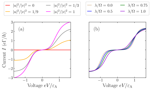
Supplementary Figure S1: Current $I$ of boson-coupled ABSs vs voltage $V$ calculated using the rate equation [Eq. (5) of the main text] for (a) different ratios of PH components $|u|^{2}/|v|^{2}$ with $\lambda/\Omega=1$ and (b) different ABS-boson coupling strengths $\lambda$ with $|u|^{2}/|v|^{2}=1/3$. The conductance calculated from the above current is shown in Fig. 2 of the main text. The parameters for all panels are: $\varepsilon_{\mathrm{A}}/\Omega=3$, $\Gamma/\Omega=0.05/(2\pi)$, and $k_{\mathrm{B}}T/\Omega=0.4$.

Supplementary Figure S2: Current $I$ of boson-coupled ABSs vs voltage $V$ calculated using the mean-field Keldysh approach [Eq. (8) of the main text] for (a) different ratios of PH components $|u|^{2}/|v|^{2}$ with $\lambda/\Omega=1$ and (b) different ABS-boson coupling strengths $\lambda$ with $|u|^{2}/|v|^{2}=1/3$. The conductance calculated from the above current is shown in Fig. 3 of the main text. Inset: Expectation value of the boson displacement operator $\langle\hat{x}\rangle$ vs voltage $V$ calculated self-consistently using Eq. (10) of the main text. The parameters for all panels are: $\varepsilon_{\mathrm{A}}/\Omega=3$, $\Gamma/\Omega=2$, and $k_{\mathrm{B}}T/\Omega=0.4$.

VI Dependence of the current and conductance calculated from the rate equation on ABS-boson coupling strength, temperature, boson frequency, and ABS energy

Figure S3 shows the current (upper panels) and conductance (lower panels) of boson-coupled ABSs calculated from the rate equation [Eq. (5) of the main text] for different ABS-boson coupling strengths $\lambda$ [Figs. S3(a,b)], temperatures $T$ [Figs. S3(c,d)], boson frequencies $\Omega$ [Figs. S3(e,f)] and ABS energies $\varepsilon_{\mathrm{A}}$ [Figs. S3(g,h)]. Figure S3(b) shows that the magnitude of the conductance PH asymmetry $\zeta$ has a nonmonotonic dependence on the ABS-boson coupling strength $\lambda$. In the limit $\varepsilon_{\mathrm{A}}-\lambda^{2}/\Omega\gg k_{\mathrm{B}}T$ (where the two conductance peaks are well separated), the conductance PH asymmetry $\zeta$ increases with increasing $\lambda$; this corresponds to the results shown in Fig. 2(b) of the main text. As $\lambda$ keeps increasing, the two conductance peaks approach each other and in the regime where $\varepsilon_{\mathrm{A}}-\lambda^{2}/\Omega<k_{\mathrm{B}}T$, the two peaks start to overlap with each other and $\zeta$ decreases with increasing $\lambda$. Note that in the regime where $\varepsilon_{\mathrm{A}}-\lambda^{2}/\Omega>0$, the higher peak is at positive voltage for the case where $|u|^{2}>|v|^{2}$ while for the case where $|v|^{2}>|u|^{2}$, the higher peak is at negative voltage. When $\varepsilon_{\mathrm{A}}-\lambda^{2}/\Omega=0$, the two conductance peaks merge at the zero voltage which gives a zero conductance PH asymmetry ($\zeta=0$). Increasing $\lambda$ beyond this point splits the peaks but with the low and high peaks now switching sides which in turn changes the sign of $\zeta$. As $\lambda$ increases further, the two peaks move away from each other and the PH asymmetry $\zeta$ increases in magnitude; beyond a certain value of $\lambda$, $\zeta$ becomes weakly dependent on $\lambda$ as shown in the inset of Fig. S3(b). Note that for large enough $\lambda$, the position of the conductance peaks are no longer PH symmetric [see green curve in Fig. S3(b)].

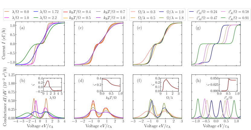
Supplementary Figure S3: Current $I$ (Upper panels) and conductance $dI/dV$ (Lower panels) of boson-coupled ABSs vs voltage $V$ calculated using the rate equation [Eq. (5) of the main text] for (a,b) different ABS-boson coupling strengths $\lambda$ with $k_{\mathrm{B}}T=0.4$, $\varepsilon_{\mathrm{A}}=3$, $\Gamma=0.05/(2\pi)$, and $\Omega=1.0$, (c,d) different temperatures $T$ with $\lambda=1.0$, $\varepsilon_{\mathrm{A}}=3.0$, $\Gamma=0.05/(2\pi)$, and $\Omega=1.0$, (e,f) different boson frequencies $\Omega$ with $k_{\mathrm{B}}T=0.4$, $\varepsilon_{\mathrm{A}}=3.0$, $\Gamma=0.05/(2\pi)$, and $\lambda=1.0$, and (g,h) different renormalized ABS energies $\tilde{\varepsilon}_{\mathrm{A}}^{\prime}\equiv|\varepsilon_{\mathrm{A}}-\lambda^{2}/\Omega|+k_{\mathrm{B}}T/2$ with $k_{\mathrm{B}}T=0.4$, $\lambda=3.0$ and $\Gamma=1/(40\pi)$, and $\Omega=9.0$. Inset: (b) Conductance PH asymmetry $\zeta$ vs $\lambda/\Omega$, (d) $\zeta$ vs temperature $T$, (f) $\zeta$ vs boson frequency $\Omega$, and (h) $\zeta$ vs $\tilde{\varepsilon}_{\mathrm{A}}^{\prime}/\Omega$. Panel (h) shows that the subgap conductances exhibit PH asymmetry only for $\tilde{\varepsilon}_{\mathrm{A}}^{\prime}/\Omega\gtrsim 0.5$ where $\tilde{\varepsilon}_{\mathrm{A}}^{\prime}\equiv|\varepsilon_{\mathrm{A}}-\lambda^{2}/\Omega|+k_{\mathrm{B}}T/2$. The parameters used for all panels are: $|u|^{2}/|v|^{2}=1/9$.

Figure S3(d) shows that the conductance PH asymmetry $\zeta$ decreases with increasing temperature $T$. This is due to the fact that temperature broadens the conductance peaks. The dependence of the ABS conductance on the boson frequency $\Omega$ is shown in Fig. S3(f). The PH asymmetry $\zeta$ has a nonmonotonic behavior with the boson frequency $\Omega$ where it first increases with increasing $\Omega$ and then after reaching its maximum, it decreases with increasing $\Omega$. The initial increase of $\zeta$ with increasing $\Omega$ can be attributed to the fact that the two conductance peaks move away from each other as $\Omega$ increases ($\tilde{\varepsilon}_{\mathrm{A}}=\varepsilon_{\mathrm{A}}-\lambda^{2}/\Omega$ increases with increasing $\Omega$). The decrease of $\zeta$ for large $\Omega$ is due to the fact that the effective ABS-boson coupling strength $\lambda/\Omega$ decreases with increasing $\Omega$. Figure S3(h) shows the dependence of the conductance on the ABS energy. As shown in the inset of panel (h), the peak conductance only exhibits the PH asymmetry for $\Omega\lesssim 2|\tilde{\varepsilon}_{\mathrm{A}}|+k_{\mathrm{B}}T$. This can be understood from the fact that the second tunneling process [whose rate is $R^{1\rightarrow 0;e}$ in Fig. 1(a) or $R^{1\rightarrow 0;h}$ in Fig. 1(b) of the main text] can transfer lead electrons or holes with an energy difference up to $\sim 2|\tilde{\varepsilon}_{\mathrm{A}}|+k_{\mathrm{B}}T$ from the subgap state, where this energy difference is transferred in form of boson energy $\Omega$. Even though in this paper, we focus only on the regime $k_{\mathrm{B}}T\gtrsim\lambda$ where the boson sidebands vanish due to the thermal broadening Mitra et al. (2004), the dependence of the ABS conductance peak on the above parameters also hold true in the case where there are boson sidebands. Moreover, the PH asymmetry of the boson sidebands also have similar dependences on the above parameters as that of the ABS conductance peak.

VII Derivation of the current in the Keldysh formalism

In this section, we derive the current [Eq. (8) of the main text] following Refs. Cuevas et al. (1996); González et al. (2020); Ruby et al. (2015). We begin by writing the Hamiltonian as

$$\hat{H}=\hat{H}_{\mathrm{A}}+\hat{H}_{\mathrm{L}}+\hat{H}_{\mathrm{T}},$$ (S-34)

where

$$\hat{H}_{\mathrm{A}} =(\varepsilon_{\mathrm{A}}+\sqrt{2}\lambda\langle\hat{x}\rangle)\hat{\gamma}^{\dagger}\hat{\gamma},$$ (S-35a)

$$\hat{H}_{\mathrm{L}} =\sum_{k}\varepsilon_{\mathrm{L},k}\hat{c}_{\mathrm{L},k}^{\dagger}\hat{c}_{\mathrm{L},k},$$ (S-35b)

$$\hat{H}_{\mathrm{T}} =t\hat{c}_{\mathrm{L}}^{\dagger}\hat{d}_{\mathrm{A}}+\mathrm{H.c.}$$ (S-35c)

In Eq. (S-35a), $\hat{H}_{\mathrm{A}}$ is the mean-field Hamiltonian of the ABS-boson system obtained by replacing $\hat{x}$ in Eq. (7) of the main text by $\langle\hat{x}\rangle$ where $\langle\hat{x}\rangle=\frac{\langle\hat{b}+\hat{b}^{\dagger}\rangle}{\sqrt{2}}$ is the mean-field boson displacement. Note that we have dropped the constant in the Hamiltonian $\hat{H}_{\mathrm{A}}$ in Eq. (S-35a) since this is just a shift in the energy. To calculate the current, we first apply a gauge transformation Rogovin and Scalapino (1974)

$$\hat{U}(\tau)=\mathrm{exp}\left\{\frac{i}{\hbar}\int_{0}^{\tau}d\tau^{\prime}[\mu_{\mathrm{L}}(\tau^{\prime})\hat{N}_{\mathrm{L}}+\mu_{\mathrm{S}}(\tau^{\prime})\hat{N}_{\mathrm{S}}]\right\},$$ (S-36)

to the Hamiltonian $\hat{H}$ in Eq. (S-34), where $\hat{N}_{\mathrm{L}}=\hat{c}_{\mathrm{L}}^{\dagger}\hat{c}_{\mathrm{L}}$ and $N_{\mathrm{S}}=\hat{d}_{\mathrm{A}}^{\dagger}\hat{d}_{\mathrm{A}}$ are the lead and substrate electron number, respectively, with $\hat{d}_{\mathrm{A}}=u\hat{\gamma}+v\hat{\gamma}^{\dagger}$. With this transformation, the single-particle energies in the lead and substrate are measured from the chemical potential of the lead ($\mu_{\mathrm{L}}$) and substrate ($\mu_{\mathrm{S}}$), respectively, where the transformed Hamiltonian is

$$\hat{\grave{H}} =\hat{U}\hat{H}\hat{U}^{\dagger}-i\hbar\hat{U}\partial_{\tau}\hat{U}^{\dagger}$$

$$=(\hat{H}_{\mathrm{L}}-\mu_{\mathrm{L}}\hat{N}_{\mathrm{L}})+(\hat{H}_{\mathrm{A}}-\mu_{\mathrm{S}}\hat{N}_{\mathrm{S}})+\hat{U}\hat{H}_{\mathrm{T}}\hat{U}^{\dagger},$$ (S-37)

with the tunneling Hamiltonian transformed as

$$\hat{\grave{H}}_{\mathrm{T}} =\hat{U}\hat{H}_{\mathrm{T}}\hat{U}^{\dagger}$$

$$=te^{ieV\tau/\hbar}\hat{c}_{\mathrm{L}}^{\dagger}\hat{d}_{\mathrm{A}}+\mathrm{H.c.},$$ (S-38)

where $eV=\mu_{\mathrm{L}}-\mu_{\mathrm{S}}$.

The current operator is given by

$$\hat{I}=e\dot{\hat{N}}_{\mathrm{L}}=ie[\hat{N}_{\mathrm{L}},\hat{\grave{H}}_{\mathrm{T}}]=i\frac{e}{\hbar}\left(te^{ieV\tau/\hbar}\hat{c}_{\mathrm{L}}^{\dagger}\hat{d}_{\mathrm{A}}-\mathrm{H.c.}\right).$$ (S-39)

By taking the expectation value of the current operator, we have

$$I(\tau) =\frac{e}{2h}\mathrm{Tr}\left\{\sigma_{z}[\grave{t}(\tau)G^{<}_{\mathrm{A}\mathrm{L}}(\tau,\tau)-G^{<}_{\mathrm{L}\mathrm{A}}(\tau,\tau)\grave{t}^{\dagger}(\tau)]\right\},$$ (S-40)

where $\sigma_{z}$ is the $z$-Pauli Matrix in the Nambu basis. In Eq. (S-40), we have introduced the hopping matrix

$$\grave{t}(\tau)=e^{ieV\tau/\hbar\sigma_{z}}\check{t}=t\left(\begin{matrix}ue^{ieV\tau/\hbar}&ve^{ieV\tau/\hbar}\\ -v^{*}e^{-ieV\tau/\hbar}&-u^{*}e^{-ieV\tau/\hbar}\end{matrix}\right),$$ (S-41)

and the lesser Green’s function in the Nambu space [$(G^{<}_{\alpha\beta})_{ij}=i\langle\Psi^{\dagger}_{\beta j}\Psi_{\alpha i}\rangle$] with $i,j=\mathrm{L},\mathrm{A}$ denoting the quantities for the lead and ABS, respectively, where $\Psi_{\mathrm{L}}=(\hat{c}_{\mathrm{L}},\hat{c}_{\mathrm{L}}^{\dagger})^{T}$ and $\Psi_{\mathrm{A}}=(\hat{\gamma},\hat{\gamma}^{\dagger})^{T}$. We can Fourier-expand the current and Green’s functions in terms of the frequency $\omega_{0}=eV/\hbar$, where we have

$$I(\tau) =\sum_{n}I_{n}e^{in\omega_{0}\tau},$$ (S-42a)

$$G(\tau_{1},\tau_{2}) =\sum_{n}e^{in\omega_{0}\tau_{2}}\int_{-\infty}^{\infty}\frac{d\omega}{2\pi}e^{-i\omega(\tau_{1}-\tau_{2})}G(\omega,\omega+n\omega_{0}).$$ (S-42b)

Let us denote $G_{mn}(\omega)\equiv G(\omega+m\omega_{0},\omega+n\omega_{0})$ for which we have $G_{mn}(\omega)=G_{m-n,0}(\omega+n\omega_{0})$.

The dc current which is the zeroth order ($I_{0}$) in the Fourier expansion of the current [Eq. (S-42a)] is given by

$$I_{0}=\frac{e}{2h}t\int d\omega \left(ue^{i\omega_{0}\tau}G^{<,ee}_{\mathrm{AL},10}+ve^{i\omega_{0}\tau}G^{<,he}_{\mathrm{AL},10}+v^{*}e^{-i\omega_{0}\tau}G^{<,eh}_{\mathrm{AL},-1,0}+u^{*}e^{-i\omega_{0}\tau}G^{<,hh}_{\mathrm{AL},-1,0}\right.$$

$$\hskip 14.22636pt\left.-u^{*}e^{-i\omega_{0}\tau}G^{<,ee}_{\mathrm{LA},01}-v^{*}e^{-i\omega_{0}\tau}G^{<,eh}_{\mathrm{LA},01}-ve^{i\omega_{0}\tau}G^{<,he}_{\mathrm{LA},0,-1}-ue^{i\omega_{0}\tau}G^{<,hh}_{\mathrm{LA},0,-1}\right),$$ (S-43)

where the superscripts $ee$, $eh$, $he$, and $hh$ denote the matrix elements in the Nambu space. Using the Langreth rule Haug and Jauho (2008)

$$G^{<}_{\mathrm{A}\mathrm{L}} =G^{r}_{\mathrm{A}}\grave{t}^{\dagger}g^{<}_{\mathrm{L}}+G^{<}_{\mathrm{A}}\grave{t}^{\dagger}g^{a}_{\mathrm{L}},$$ (S-44a)

$$G^{<}_{\mathrm{L}\mathrm{A}} =g^{r}_{\mathrm{L}}\grave{t}G^{<}_{\mathrm{A}}+g^{<}_{\mathrm{L}}\grave{t}G^{a}_{\mathrm{A}},$$ (S-44b)

where $g_{\mathrm{L}}=\mathrm{diag}\left(g_{\mathrm{L}}^{ee},g_{\mathrm{L}}^{hh}\right)$, we have

$$G^{<,ee}_{\mathrm{AL},10} =t\left[\left(G^{r,ee}_{\mathrm{A},11}u^{*}+G^{r,eh}_{\mathrm{A},11}v^{*}\right)e^{-i\omega_{0}\tau}g^{<,ee}_{\mathrm{L},00}+\left(G^{<,ee}_{\mathrm{A},11}u^{*}+G^{<,eh}_{\mathrm{A},11}v^{*}\right)e^{-i\omega_{0}\tau}g^{a,ee}_{\mathrm{L},00}\right],$$ (S-45a)

$$G^{<,hh}_{\mathrm{AL},-1,0} =-t\left[\left(G^{r,he}_{\mathrm{A},-1,-1}v+G^{r,hh}_{\mathrm{A},-1,-1}u\right)e^{i\omega_{0}\tau}g^{<,hh}_{\mathrm{L},00}+\left(G^{<,he}_{\mathrm{A},-1,-1}v+G^{<,hh}_{\mathrm{A},-1,-1}u\right)e^{i\omega_{0}\tau}g^{a,hh}_{\mathrm{L},00}\right],$$ (S-45b)

$$G^{<,he}_{\mathrm{AL},10} =t\left[\left(G^{r,he}_{\mathrm{A},11}u^{*}+G^{r,hh}_{\mathrm{A},11}v^{*}\right)e^{-i\omega_{0}\tau}g^{<,ee}_{\mathrm{L},00}+\left(G^{<,he}_{\mathrm{A},11}u^{*}+G^{<,hh}_{\mathrm{A},11}v^{*}\right)e^{-i\omega_{0}\tau}g^{a,ee}_{\mathrm{L},00}\right],$$ (S-45c)

$$G^{<,eh}_{\mathrm{AL},-1,0} =-t\left[\left(G^{r,ee}_{\mathrm{A},-1,-1}v+G^{r,eh}_{\mathrm{A},-1,-1}u\right)e^{i\omega_{0}\tau}g^{<,hh}_{\mathrm{L},00}+\left(G^{<,ee}_{\mathrm{A},-1,-1}v+G^{<,eh}_{\mathrm{A},-1,-1}u\right)e^{i\omega_{0}\tau}g^{a,hh}_{\mathrm{L},00}\right],$$ (S-45d)

$$G^{<,ee}_{\mathrm{LA},01} =t\left[g^{<,ee}_{\mathrm{L},00}e^{i\omega_{0}\tau}\left(uG^{a,ee}_{\mathrm{A},11}+vG^{a,he}_{\mathrm{A},11}\right)+g^{r,ee}_{\mathrm{L},00}e^{i\omega_{0}\tau}\left(uG^{<,ee}_{\mathrm{A},11}+vG^{<,he}_{\mathrm{A},11}\right)\right],$$ (S-45e)

$$G^{<,hh}_{\mathrm{LA},0,-1} =-t\left[g^{<,hh}_{\mathrm{L},00}e^{-i\omega_{0}\tau}\left(v^{*}G^{a,eh}_{\mathrm{A},-1,-1}+u^{*}G^{a,hh}_{\mathrm{A},-1,-1}\right)+g^{r,hh}_{\mathrm{L},00}e^{-i\omega_{0}\tau}\left(v^{*}G^{<,eh}_{\mathrm{A},-1,-1}+u^{*}G^{<,hh}_{\mathrm{A},-1,-1}\right)\right],$$ (S-45f)

$$G^{<,he}_{\mathrm{LA},0,-1} =-t\left[g^{<,hh}_{\mathrm{L},00}e^{-i\omega_{0}\tau}\left(v^{*}G^{a,ee}_{\mathrm{A},-1,-1}+u^{*}G^{a,he}_{\mathrm{A},-1,-1}\right)+g^{r,hh}_{\mathrm{L},00}e^{-i\omega_{0}\tau}\left(v^{*}G^{<,ee}_{\mathrm{A},-1,-1}+u^{*}G^{<,he}_{\mathrm{A},-1,-1}\right)\right],$$ (S-45g)

$$G^{<,eh}_{\mathrm{LA},01} =t\left[g^{<,ee}_{\mathrm{L},00}e^{i\omega_{0}\tau}\left(uG^{a,eh}_{\mathrm{A},11}+vG^{a,hh}_{\mathrm{A},11}\right)+g^{r,ee}_{\mathrm{L},00}e^{i\omega_{0}\tau}\left(uG^{<,eh}_{\mathrm{A},11}+vG^{<,hh}_{\mathrm{A},11}\right)\right].$$ (S-45h)

Substituting Eq. (S-45) into Eq. (VII) and using $g^{ee}_{\mathrm{L,00}}=g^{hh}_{\mathrm{L,00}}=g_{\mathrm{L}}$, we have

$$I_{0}=\frac{e}{2h}t^{2}\int d\omega \left\{\left[|u|^{2}(G^{r,ee}_{\mathrm{A}}(\omega_{+})-G^{a,ee}_{\mathrm{A}}(\omega_{+}))+uv^{*}(G^{r,eh}_{\mathrm{A}}(\omega_{+})-G^{a,eh}_{\mathrm{A}}(\omega_{+}))\right.\right.$$

$$\hskip 56.9055pt\left.+u^{*}v(G^{r,he}_{\mathrm{A}}(\omega_{+})-G^{a,he}_{\mathrm{A}}(\omega_{+}))+|v|^{2}(G^{r,hh}_{\mathrm{A}}(\omega_{+})-G^{a,hh}_{\mathrm{A}}(\omega_{+}))\right]g^{<}_{\mathrm{L}}(\omega)$$

$$\hskip 5.69046pt-\left[|v|^{2}(G^{r,ee}_{\mathrm{A}}(\omega_{-})-G^{a,ee}_{\mathrm{A}}(\omega_{-}))+uv^{*}(G^{r,eh}_{\mathrm{A}}(\omega_{-})-G^{a,eh}_{\mathrm{A}}(\omega_{-}))\right.$$

$$\hskip 56.9055pt\left.+u^{*}v(G^{r,he}_{\mathrm{A}}(\omega_{-})-G^{a,he}_{\mathrm{A}}(\omega_{-}))+|u|^{2}(G^{r,hh}_{\mathrm{A}}(\omega_{-})-G^{a,hh}_{\mathrm{A}}(\omega_{-}))\right]g^{<}_{\mathrm{L}}(\omega)$$

$$\hskip 5.69046pt+\left[|u|^{2}G^{<,ee}_{\mathrm{A}}(\omega_{+})+uv^{*}G^{<,eh}_{\mathrm{A}}(\omega_{+})+u^{*}vG^{<,he}_{\mathrm{A}}(\omega_{+})+|v|^{2}G^{<,hh}_{\mathrm{A}}(\omega_{+})\right]\left[g^{a}_{\mathrm{L}}(\omega)-g^{r}_{\mathrm{L}}(\omega)\right]$$

$$\hskip 5.69046pt-\left.\left[|v|^{2}G^{<,ee}_{\mathrm{A}}(\omega_{-})+uv^{*}G^{<,eh}_{\mathrm{A}}(\omega_{-})+u^{*}vG^{<,he}_{\mathrm{A}}(\omega_{-})+|u|^{2}G^{<,hh}_{\mathrm{A}}(\omega_{-})\right]\left[g^{a}_{\mathrm{L}}(\omega)-g^{r}_{\mathrm{L}}(\omega)\right]\right\}.$$ (S-46)

Furthermore, by using the relation $G^{<}-G^{>}=G^{a}-G^{r}$, we obtain

$$I_{0}=\frac{e}{2h}t^{2}\int d\omega \left\{\left[|u|^{2}G^{>,ee}_{\mathrm{A}}(\omega)+uv^{*}G^{>,eh}_{\mathrm{A}}(\omega)+u^{*}vG^{>,he}_{\mathrm{A}}(\omega)+|v|^{2}G^{>,hh}_{\mathrm{A}}(\omega)\right]g^{<}_{\mathrm{L}}(\omega_{-})\right.$$

$$\hskip 5.69046pt-\left[|v|^{2}G^{>,ee}_{\mathrm{A}}(\omega)+uv^{*}G^{>,eh}_{\mathrm{A}}(\omega)+u^{*}vG^{>,he}_{\mathrm{A}}(\omega)+|u|^{2}G^{>,hh}_{\mathrm{A}}(\omega)\right]g^{<}_{\mathrm{L}}(\omega_{+})$$

$$\hskip 5.69046pt-\left[|u|^{2}G^{<,ee}_{\mathrm{A}}(\omega)+uv^{*}G^{<,eh}_{\mathrm{A}}(\omega)+u^{*}vG^{<,he}_{\mathrm{A}}(\omega)+|v|^{2}G^{<,hh}_{\mathrm{A}}(\omega)\right]g^{>}_{\mathrm{L}}(\omega_{-})$$

$$\hskip 5.69046pt\left.+\left[|v|^{2}G^{<,ee}_{\mathrm{A}}(\omega)+uv^{*}G^{<,eh}_{\mathrm{A}}(\omega)+u^{*}vG^{<,he}_{\mathrm{A}}(\omega)+|u|^{2}G^{<,hh}_{\mathrm{A}}(\omega)\right]g^{>}_{\mathrm{L}}(\omega_{+})\right\}.$$ (S-47)

The current can be written more compactly as

$$I =\frac{e}{2h}\int d\omega\mathrm{Tr}\left[G^{>}_{\mathrm{A}}(\omega)\widetilde{\Sigma}_{\mathrm{A}}^{<}(\omega)-G^{<}_{\mathrm{A}}(\omega)\widetilde{\Sigma}_{\mathrm{A}}^{>}(\omega)\right],$$ (S-48)

where

$$\widetilde{\Sigma}^{<,>}_{\mathrm{A}}(\omega) =\check{t}^{\dagger}\left(\begin{matrix}g_{\mathrm{L}}^{<,>}(\omega_{-})&0\\ 0&-g_{\mathrm{L}}^{<,>}(\omega_{+})\end{matrix}\right)\check{t}$$

$$=t^{2}\left(\begin{matrix}u^{*}&-v\\ v^{*}&-u\end{matrix}\right)\left(\begin{matrix}g_{\mathrm{L}}^{<,>}(\omega_{-})&0\\ 0&-g_{\mathrm{L}}^{<,>}(\omega_{+})\end{matrix}\right)\left(\begin{matrix}u&v\\ -v^{*}&-u^{*}\end{matrix}\right)$$

$$=t^{2}\left(\begin{matrix}|u|^{2}g_{\mathrm{L}}^{<,>}(\omega_{-})-|v|^{2}g_{\mathrm{L}}^{<,>}(\omega_{+})&vu^{*}\left[g_{\mathrm{L}}^{<,>}(\omega_{-})-g_{\mathrm{L}}^{<,>}(\omega_{+})\right]\\ uv^{*}\left[g_{\mathrm{L}}^{<,>}(\omega_{-})-g_{\mathrm{L}}^{<,>}(\omega_{+})\right]&|v|^{2}g_{\mathrm{L}}^{<,>}(\omega_{-})-|u|^{2}g_{\mathrm{L}}^{<,>}(\omega_{+})\end{matrix}\right),$$ (S-49)

with $g^{<}_{\mathrm{L}}(\omega)=f(\omega)(g^{a}_{\mathrm{L}}(\omega)-g^{r}_{\mathrm{L}}(\omega))$, $g^{>}_{\mathrm{L}}(\omega)=-(1-f(\omega))(g^{a}_{\mathrm{L}}(\omega)-g^{r}_{\mathrm{L}}(\omega))$ and $g^{r}_{\mathrm{L}}(\omega_{-})=g^{r}_{\mathrm{L}}(\omega_{+})\equiv-i\pi\nu_{0}$, where where $\nu_{0}$ is the density of states at the lead Fermi energy. Substituting the expressions for $\widetilde{\Sigma}^{<,>}_{\mathrm{A}}(\omega)$ [Eqs. (VII)], $G^{<}_{\mathrm{A}}(\omega)$ [Eqs. (S-57)], and the corresponding equations for $G^{>}_{\mathrm{A}}(\omega)$ into Eq. (S-48), we obtain Eq. (8) of the main text:

$$I(V)=\frac{e}{h}\Gamma^{2}\int d\omega\mathcal{A}(\omega)[f(\omega_{-})-f(\omega_{+})],$$ (S-50)

where

$$\mathcal{A}(\omega)=\frac{4|uv|^{2}}{\left[\omega-\frac{(\varepsilon_{\mathrm{A}}+\sqrt{2}\lambda\langle\hat{x}\rangle)^{2}}{\omega}-\frac{(\Gamma_{u}-\Gamma_{v})^{2}}{4\omega}\right]^{2}+(\Gamma_{u}+\Gamma_{v})^{2}},$$ (S-51)

with $\Gamma_{u}=\Gamma|u|^{2}$ and $\Gamma_{v}=\Gamma|v|^{2}$. Note that the term $\langle\hat{x}\rangle$ is evaluated self-consistently using

$$\langle\hat{x}\rangle =-\frac{\sqrt{2}\lambda}{\Omega}\langle\hat{\gamma}^{\dagger}(\tau)\hat{\gamma}(\tau)\rangle=i\frac{\sqrt{2}\lambda}{\Omega}\int\frac{d\omega}{2\pi}G^{<,ee}_{\mathrm{A}}(\omega),$$ (S-52)

or Eq. (10) of the main text:

$$\langle\hat{x}\rangle =-\frac{\sqrt{2}\lambda}{\Omega}\langle\hat{\gamma}^{\dagger}(\tau)\hat{\gamma}(\tau)\rangle=-\frac{\lambda}{\sqrt{2}\Omega}\left(1+\langle\hat{\gamma}^{\dagger}(\tau)\hat{\gamma}(\tau)\rangle-\langle\hat{\gamma}(\tau)\hat{\gamma}^{\dagger}(\tau)\rangle\right)=-\frac{\lambda}{\sqrt{2}\Omega}\left\{1-i\int\frac{d\omega}{2\pi}\mathrm{Tr}\left[G^{<}_{\mathrm{A}}(\omega)\sigma_{z}\right]\right\}.$$ (S-53)

VIII Explicit expressions for $G_{\mathrm{A}}^{<,>}(\omega)$

In this section, we evaluate the expressions for the ABS lesser and greater Green’s functions $G_{\mathrm{A}}^{<,>}(\omega)$ which are used to calculate the current [Eq. (8) of the main text] and the expectation value of the boson displacement operator $\langle\hat{x}\rangle$ [Eq. (10) of the main text]. Using the Fourier expansion as in Eq. (S-42b), we can relate the ABS lesser and greater Green’s function in the frequency domain $G_{\mathrm{A}}^{<,>}(\omega)$ to their time-domain counterparts Haug and Jauho (2008), i.e.,

$$G^{<}_{\mathrm{A}}(\tau_{1},\tau_{2}) =\left(\begin{matrix}G^{<,ee}_{\mathrm{A}}(\tau_{1},\tau_{2})&G^{<,eh}_{\mathrm{A}}(\tau_{1},\tau_{2})\\ G^{<,he}_{\mathrm{A}}(\tau_{1},\tau_{2})&G^{<,hh}_{\mathrm{A}}(\tau_{1},\tau_{2})\end{matrix}\right)\equiv i\left(\begin{matrix}\langle\gamma^{\dagger}(\tau_{2})\gamma(\tau_{1})\rangle&\langle\gamma(\tau_{2})\gamma(\tau_{1})\rangle\\ \langle\gamma^{\dagger}(\tau_{2})\gamma^{\dagger}(\tau_{1})\rangle&\langle\gamma(\tau_{2})\gamma^{\dagger}(\tau_{1})\rangle\end{matrix}\right),$$ (S-54a)

$$G^{>}_{\mathrm{A}}(\tau_{1},\tau_{2}) =\left(\begin{matrix}G^{>,ee}_{\mathrm{A}}(\tau_{1},\tau_{2})&G^{>,eh}_{\mathrm{A}}(\tau_{1},\tau_{2})\\ G^{>,he}_{\mathrm{A}}(\tau_{1},\tau_{2})&G^{>,hh}_{\mathrm{A}}(\tau_{1},\tau_{2})\end{matrix}\right)\equiv-i\left(\begin{matrix}\langle\gamma(\tau_{1})\gamma^{\dagger}(\tau_{2})\rangle&\langle\gamma^{\dagger}(\tau_{1})\gamma^{\dagger}(\tau_{2})\rangle\\ \langle\gamma(\tau_{1})\gamma(\tau_{2})\rangle&\langle\gamma^{\dagger}(\tau_{1})\gamma(\tau_{2})\rangle\end{matrix}\right).$$ (S-54b)

To evaluate $G_{\mathrm{A}}^{<,>}(\omega)$, we begin by writing the ABS Green’s function in the Lehmann representation as

$$g_{\mathrm{A}}(\omega) =\frac{\Phi_{+}\Phi^{\dagger}_{+}}{\omega-(\varepsilon_{\mathrm{A}}+\sqrt{2}\lambda\langle\hat{x}\rangle)}+\frac{\Phi_{-}\Phi^{\dagger}_{-}}{\omega+(\varepsilon_{\mathrm{A}}+\sqrt{2}\lambda\langle\hat{x}\rangle)}.$$ (S-55)

where $\Phi_{+}=(1,0)^{T}$ and $\Phi_{-}=(0,1)^{T}$ are the positive- and negative-energy eigenfunction of the ABS written in the Nambu basis $(\hat{\gamma},\hat{\gamma}^{\dagger})^{T}$. The ABS’s self energy due to the lead coupling is $\Sigma^{r}_{\mathrm{A}}(\omega)=\check{t}^{\dagger}\mathrm{diag}(g_{L}^{r}(\omega_{-}),g_{L}^{r}(\omega_{+}))\check{t}$ where $\check{t}=t\left(\begin{matrix}u&v\\ -v^{*}&-u^{*}\end{matrix}\right)$ is the hopping matrix, and $g^{r}_{\mathrm{L}}(\omega_{-})=g^{r}_{\mathrm{L}}(\omega_{+})=-i\pi\nu_{0}$ is the lead retarded Green’s function with $\omega_{\pm}=\omega\pm eV$. Similar relations apply for $\Sigma_{\mathrm{A}}^{a,<,>}(\omega)$. The ABS lesser Green’s function is Haug and Jauho (2008)

$$~{}G^{<}_{\mathrm{A}}(\omega) =g^{<}_{\mathrm{A}}(\omega)+g^{r}_{\mathrm{A}}(\omega)\Sigma^{r}_{\mathrm{A}}(\omega)G^{<}_{\mathrm{A}}(\omega)+\left[g^{r}_{\mathrm{A}}(\omega)\Sigma^{<}_{\mathrm{A}}(\omega)+g^{<}_{\mathrm{A}}(\omega)\Sigma^{a}_{\mathrm{A}}(\omega)\right]G^{a}_{\mathrm{A}}(\omega)$$

$$=\frac{1}{1-g^{r}_{\mathrm{A}}(\omega)\Sigma^{r}_{\mathrm{A}}(\omega)}\left[g^{<}_{\mathrm{A}}(\omega)\left(1+\Sigma^{a}_{\mathrm{A}}(\omega)G^{a}_{\mathrm{A}}(\omega)\right)+g^{r}_{\mathrm{A}}(\omega)\Sigma^{<}_{\mathrm{A}}(\omega)G^{a}_{\mathrm{A}}(\omega)\right],$$ (S-56)

where $G^{r,a}_{\mathrm{A}}=g^{r,a}_{\mathrm{A}}(1-g^{r,a}_{\mathrm{A}}\Sigma^{r,a}_{\mathrm{A}})^{-1}$, $g^{<}_{j}(\omega)=f(\omega)(g^{a}_{j}-g^{r}_{j})$ and $g^{>}_{j}(\omega)=-(1-f(\omega))(g^{a}_{j}-g^{r}_{j})$ with $j$ = L, A. The explicit expressions of the matrix elements of $G^{<}_{\mathrm{A}}(\omega)=\left(\begin{matrix}G^{<,ee}_{\mathrm{A}}(\omega)&G^{<,eh}_{\mathrm{A}}(\omega)\\ G^{<,he}_{\mathrm{A}}(\omega)&G^{<,hh}_{\mathrm{A}}(\omega)\end{matrix}\right)$ can be evaluated as

$$G^{<,ee}_{\mathrm{A}}(\omega) =\frac{i}{D}\left\{\left[\Gamma_{u}f(\omega_{-})+\Gamma_{v}f(\omega_{+})\right]\left[\left(\omega+\varepsilon_{\mathrm{A}}+\sqrt{2}\lambda\langle\hat{x}\rangle\right)^{2}+\left(\frac{\Gamma_{u}-\Gamma_{v}}{2}\right)^{2}\right]\right\},$$ (S-57a)

$$G^{<,eh}_{\mathrm{A}}(\omega) =\frac{i}{D}\left\{\Gamma u^{*}v\left[\left(f(\omega_{+})+f(\omega_{-})\right)\left(\omega^{2}-(\varepsilon_{\mathrm{A}}+\sqrt{2}\lambda\langle\hat{x}\rangle)^{2}-\left(\frac{\Gamma_{u}-\Gamma_{v}}{2}\right)^{2}\right)+i\omega\left(f(\omega_{+})-f(\omega_{-})\right)\left(\Gamma_{u}-\Gamma_{v}\right)\right]\right\},$$ (S-57b)

$$G^{<,he}_{\mathrm{A}}(\omega) =\frac{i}{D}\left\{\Gamma uv^{*}\left[\left(f(\omega_{+})+f(\omega_{-})\right)\left(\omega^{2}-(\varepsilon_{\mathrm{A}}+\sqrt{2}\lambda\langle\hat{x}\rangle)^{2}-\left(\frac{\Gamma_{u}-\Gamma_{v}}{2}\right)^{2}\right)-i\omega\left(f(\omega_{+})-f(\omega_{-})\right)\left(\Gamma_{u}-\Gamma_{v}\right)\right]\right\},$$ (S-57c)

$$G^{<,hh}_{\mathrm{A}}(\omega) =\frac{i}{D}\left\{\left[\Gamma_{u}f(\omega_{+})+\Gamma_{v}f(\omega_{-})\right]\left[\left(\omega-(\varepsilon_{\mathrm{A}}+\sqrt{2}\lambda\langle\hat{x}\rangle)\right)^{2}+\left(\frac{\Gamma_{u}-\Gamma_{v}}{2}\right)^{2}\right]\right\},$$ (S-57d)

where $\omega_{\pm}=\omega\pm eV$ and

$$D =\left[\omega^{2}-(\varepsilon_{\mathrm{A}}+\sqrt{2}\lambda\langle\hat{x}\rangle)^{2}-\frac{(\Gamma_{u}-\Gamma_{v})^{2}}{4}\right]^{2}+\omega^{2}(\Gamma_{u}+\Gamma_{v})^{2},$$ (S-58)

with $\Gamma_{u}=\Gamma|u|^{2}$ and $\Gamma_{v}=\Gamma|v|^{2}$. The expressions for the matrix elements of the ABS greater Green’s function $G^{>}_{\mathrm{A}}(\omega)$ can be obtained from Eq. (S-57) by using the substitutions: $f(\omega_{-})\rightarrow f(\omega_{-})-1$ and $f(\omega_{+})\rightarrow f(\omega_{+})-1$.

IX Dependence of the current and conductance calculated from Keldysh approach on ABS-boson coupling strength, temperature, boson frequency, and lead-tunnel coupling strength

Figure S4 shows the current (upper panels) and conductance (lower panels) of boson-coupled ABSs calculated from the Keldysh approach [Eq. (8) of the main text] subject to the self-consistency condition [Eq. (10) of the main text]. The plots are shown for different ABS-boson coupling strengths $\lambda$ [Figs. S4(a,b)], temperatures $T$ [Figs. S4(c,d)], boson frequencies $\Omega$ [Figs. S4(e,f)] and lead-tunnel coupling strengths $\Gamma$ [Figs. S4(g,h)]. While in Fig. 3 of the main text, we have shown that the PHS breaking holds for the case of low-frequency bosons, here we will show that it also holds for the case of high-frequency bosons, i.e., $\Omega>2\varepsilon_{\mathrm{A}}+k_{\mathrm{B}}T$. Unlike the perturbative calculation in the rate equation, the PHS breaking calculated from the Keldysh approach arises due to non-perturbative effects of tunneling, i.e., the PH asymmetry of the mean-field boson displacement value $\langle\hat{x}\rangle$. In the non-perturbative regime, electrons can tunnel from the lead into virtual states in the superconductor by emitting or absorbing bosons with high frequencies where energy violation is allowed for sufficiently large tunnel coupling ($\Gamma\gtrsim\Omega$), resulting in PHS breaking of subgap conductances. This energy violation is allowed as long as the energy violation in the first tunneling process is negated by the second tunneling process which the conserves the total energy of a full cycle of transferring a pair of electrons in the two-step tunneling process.

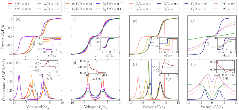
Supplementary Figure S4: Current $I$ (Upper panels) and conductance $dI/dV$ (Lower panels) of boson-coupled ABSs vs voltage $V$ calculated using the Keldysh approach [Eq. (8) of the main text] subject to the self-consistency condition [Eq. (10) of the main text]. The plots are for (a,b) different ABS-boson coupling strengths $\lambda$ with $k_{\mathrm{B}}T=0.4$, $\varepsilon_{\mathrm{A}}=3.0$, and $\Gamma=1.0$, (c,d) different temperatures $T$ with $\lambda=1.0$, $\varepsilon_{\mathrm{A}}=3.0$, and $\Gamma=1.0$, (e,f) different boson frequencies $\Omega$ with $k_{\mathrm{B}}T=0.4$, $\varepsilon_{\mathrm{A}}=3.0$, $\lambda=1.0$ and $\Gamma=1.0$, and (g,h) different lead-tunnel coupling strengths $\Gamma$ with $k_{\mathrm{B}}T=0.4$, $\lambda=1.0$ and $\varepsilon_{\mathrm{A}}=3.0$. Inset in upper panels: (a) Mean-field boson displacement value $\langle\hat{x}\rangle$ vs $\lambda/\Omega$, (c) $\langle\hat{x}\rangle$ vs temperature $T$, (e) $\langle\hat{x}\rangle$ vs boson frequency $\Omega$, and (g) $\langle\hat{x}\rangle$ vs $\Gamma/\Omega$. Inset in lower panels: (b) Conductance PH asymmetry $\zeta$ vs $\lambda/\Omega$, (d) $\zeta$ vs temperature $T$, (f) $\zeta$ vs boson frequency $\Omega$, and (h) $\zeta$ vs $\Gamma/\Omega$. The parameters used for all panels are: $|u|^{2}/|v|^{2}=1/9$. Note that for panels (a,b,c,d,g,h), we use high-frequency bosons ($\Omega=10$) where $\Omega>2\varepsilon_{\mathrm{A}}+k_{\mathrm{B}}T$.

Figure S4(b) shows that the magnitude of the conductance PH asymmetry $\zeta$ has a nonmonotonic dependence on the ABS-boson coupling strength $\lambda$. The conductance PH asymmetry $\zeta$ first increases with increasing $\lambda$ where the two peaks approach each other until they reach a certain minimum distance. Note that for this range of $\lambda$, the higher peak is at positive voltage for the case where $|u|^{2}>|v|^{2}$ while for the case where $|v|^{2}>|u|^{2}$, the higher peak is at negative voltage. After the PH asymmetry reaches a maximum, it decreases to zero and stays there for a range of $\lambda$ where the peaks remain more or less at the same place. As $\lambda$ increases and reaches a certain value, the high and low peaks switch positions, i.e., from negative to positive voltage and vice versa. As $\lambda$ keeps increasing, the two peaks move away from each other and the magnitude of the PH asymmetry increases. For large enough $\lambda$, the positions of the conductance peaks are no longer PH symmetric [see purple curve in Fig. S4(b)]. Note that the results for large $\lambda$ may not be reliable as our mean-field treatment of interactions may break down in this regime.

Figure S4(d) shows that the conductance PH asymmetry $\zeta$ decreases with increasing temperature $T$ due the temperature broadening of the conductance peaks. The dependence of the ABS conductance on the boson frequency $\Omega$ is shown in Fig. S4(f). The PH asymmetry $\zeta$ has a nonmonotonic behavior with the boson frequency $\Omega$ where its magnitude first decreases to zero with increasing $\Omega$. This corresponds to the two conductance peaks moving towards each other as $\Omega$ increases which is due to the decrease in the effective ABS-boson coupling strength $\lambda/\Omega$. After the PH asymmetry reaches zero, it switches sign which corresponds to the high and low peaks switching sides. As $\Omega$ increases, the two peaks move towards each other and the PH asymmetry increases to a certain maximum value. Having reached its maximum, the PH asymmetry $\zeta$ decreases with increasing $\Omega$ which corresponds to the decrease in the effective ABS-boson coupling strength $\lambda/\Omega$. Figure S4(h) shows the dependence of the conductance on the lead tunnel coupling $\Gamma$. As shown in the inset of panel (h), the PH asymmetry $\zeta$ has a non-monotonic dependence on the lead-tunnel coupling $\Gamma$ where it first decreases as $\Gamma$ increases. After the PH asymmetry reaches zero, it changes sign and increases in magnitude to a certain maximum value as $\Gamma$ increases. Having reached its maximum, the PH asymmetry then decreases as $\Gamma$ increases. Note that unlike the rate equation, our mean-field Keldysh approach shows that the conductance in the tunneling limit ($\Gamma/\Omega\ll 1$) still exhibits PH asymmetry even for high-frequency bosons. Since the treatment of interactions within the rate equation is exact in the tunneling limit, our Keldysh results obtained using the mean-field treatment of interactions may not be correct in this tunneling limit. This is because the mean-field approximation breaks down in this limit due to the singularity in the tunneling density of states. For the case where the tunnel coupling is not too small, the mean-field approximation is valid and we can see from Fig. S4(d) that unlike the rate equation, that subgap conductance calculated from the Keldysh approach can still be PH asymmetric for high-frequency boson case. Finally we note that since we ignore the Fock term in the mean-field approximation, the conductance calculated from the Keldysh approach has no boson sidebands.

X Details on Model II. boson-assisted tunneling model into ABS

In this section, we consider a boson-assisted tunneling Hamiltonian of the form

$$\hat{H}_{\mathrm{T}}=t(\hat{b}+\hat{b}^{\dagger})\hat{c}_{\mathrm{L}}^{\dagger}\hat{d}_{\mathrm{A}}+\mathrm{H.c.}$$ (S-59)

This tunneling Hamiltonian can be obtained by first projecting the microscopic Hamiltonian [Eq. (I)] onto the lowest and second-lowest energy sector $\alpha,\beta=1,2$ and followed by integrating out the second-lowest Bogoliubov operator $\gamma_{2}$ from the total Hamiltonian of the system.

Projecting the ABS and tunneling Hamiltonian onto the lowest and second-lowest energy state gives

$$\hat{H}_{\mathrm{A}} =\sum_{\alpha=1}^{2}\varepsilon_{\alpha}\gamma^{\dagger}_{\alpha}\gamma_{\alpha}+\sum_{\alpha,\beta=1}^{2}\biggl{(}\tilde{\lambda}^{(c)}_{\alpha\beta}\gamma^{\dagger}_{\alpha}\gamma_{\beta}+\tilde{\lambda}^{(d)}_{\alpha\beta}\gamma_{\alpha}\gamma_{\beta}+\mathrm{H.c.}\biggr{)}(\hat{b}^{\dagger}+\hat{b})+\Omega(\hat{b}^{\dagger}+\hat{b}),$$ (S-60a)

$$\hat{H}_{\mathrm{T}} =\sum_{\alpha=1}^{2}t_{\alpha}\hat{c}_{\mathrm{L}}^{\dagger}\biggl{(}\sum_{\beta=1}^{2}u_{\alpha\beta}(0)\hat{\gamma}_{\beta}+v_{\alpha\beta}(0)\hat{\gamma}^{\dagger}_{\beta}\biggr{)}+\mathrm{H.c.}$$ (S-60b)

For simplicity, we will choose parameters such that the tunneling term into the lowest Bogoliubov (ABS) operator ($\gamma_{1}$ and $\gamma_{1}^{\dagger}$) vanishes where we only have the tunneling into the second lowest Bogoliubov operator ($\gamma_{2}$ and $\gamma_{2}^{\dagger}$), i.e.,

$$\hat{H}_{\mathrm{T}} =\tilde{t}\hat{c}_{\mathrm{L}}^{\dagger}\biggl{(}\tilde{u}\hat{\gamma}_{2}+\tilde{v}\hat{\gamma}^{\dagger}_{2}\biggr{)}+\mathrm{H.c.}$$ (S-61)

Note that in the above, we have defined $\tilde{t}\tilde{u}\equiv t_{2}u_{22}(0)+t_{1}u_{12}(0)$, $\tilde{t}\tilde{v}\equiv t_{2}v_{22}(0)+t_{1}v_{12}(0)$, and we have also chosen parameters such that the tunneling term into the ABS vanishes, i.e., $t_{2}v_{21}(0)+t_{1}v_{11}(0)=0$ and $t_{2}u_{21}(0)+t_{1}u_{11}(0)=0$. We note that we choose these parameters only for simplicity and our results on PHS breaking hold in general even without this simplification.

In the following, we will see that the tunneling Hamiltonian [Eq. (S-61)] and the electron-boson interaction Hamiltonian [Eq. (S-60a)] give rise to a boson-assisted tunneling into the lowest energy ABS. To this end, we will use the path integral formalism to integrate out $\gamma_{2}$. We begin by writing down the partition function of the system as

$$Z =\int_{-\infty}^{\infty}\prod_{\alpha=1}^{2}\mathcal{D}\bar{\gamma}_{\alpha}\mathcal{D}\gamma_{\alpha}\mathcal{D}\bar{c}_{\mathrm{L},k}\mathcal{D}c_{\mathrm{L},k}\mathcal{D}\bar{b}\mathcal{D}b\biggl{(}\mathrm{exp}[i(S_{\alpha}+S_{\mathrm{b}}+S_{\mathrm{L}}+S_{\text{e-b}}+S_{\mathrm{T}})]\biggr{)}$$

$$=\int_{-\infty}^{\infty}\prod_{\alpha=1}^{2}\mathcal{D}\bar{\gamma}_{\alpha}\mathcal{D}\gamma_{\alpha}\mathcal{D}\bar{c}_{\mathrm{L},k}\mathcal{D}c_{\mathrm{L},k}\mathcal{D}\bar{b}\mathcal{D}b\biggl{(}\mathrm{exp}\bigg{[}i\int_{-\infty}^{\infty}d\tau\bigg{(}\hbar\bar{\gamma}_{\alpha}\partial_{\tau}\gamma_{\alpha}+\hbar\bar{b}\partial_{\tau}b+\hbar\bar{c}_{\mathrm{L},k}\partial_{\tau}c_{\mathrm{L},k}-\varepsilon_{\alpha}\bar{\gamma}_{\alpha}\gamma_{\alpha}-\Omega\bar{b}b$$

$$\qquad\qquad\qquad\qquad-\sum_{k}\varepsilon_{\mathrm{L},k}\bar{c}_{\mathrm{L},k}c_{\mathrm{L},k}-\sum_{\beta=1,2}(\tilde{\lambda}^{(c)}_{\alpha\beta}\bar{\gamma}_{\alpha}\gamma_{\beta}+\tilde{\lambda}^{(d)}_{\alpha\beta}\gamma_{\alpha}\gamma_{\beta}+\mathrm{h.c.})(\bar{b}+b)-\tilde{t}(\tilde{u}\bar{c}_{\mathrm{L}}\gamma_{2}+\tilde{v}\bar{c}_{\mathrm{L}}\bar{\gamma}_{2}+\mathrm{H.c.})\biggr{)}\biggr{]}\biggr{)},$$ (S-62)

where the actions are given by

$$S_{\alpha} =\int d\tau\bar{\gamma}_{\alpha}(\tau)(\hbar\partial_{\tau}-\varepsilon_{\alpha})\gamma_{\alpha}(\tau),$$ (S-63a)

$$S_{\mathrm{b}} =\int d\tau\bar{b}(\tau)(\hbar\partial_{\tau}-\Omega)b(\tau),$$ (S-63b)

$$S_{\text{e-b}} =-\int d\tau\sum_{\alpha,\beta=1}^{2}(\tilde{\lambda}^{(c)}_{\alpha\beta}\bar{\gamma}_{\alpha}(\tau)\gamma_{\beta}(\tau)+\tilde{\lambda}^{(d)}_{\alpha\beta}\gamma_{\alpha}(\tau)\gamma_{\beta}(\tau)+\mathrm{H.c.})(\bar{b}(\tau)+b(\tau)),$$ (S-63c)

$$S_{\mathrm{L}} =\sum_{k}\int d\tau\bar{c}_{\mathrm{L},k}(\tau)(\hbar\partial_{\tau}-\varepsilon_{\mathrm{L},k})c_{\mathrm{L},k}(\tau),$$ (S-63d)

$$S_{\mathrm{T}} =-\int d\tau\biggl{[}\tilde{t}(\tilde{u}\bar{c}_{\mathrm{L}}(\tau)\gamma_{2}(\tau)+\tilde{v}\bar{c}_{\mathrm{L}}(\tau)\bar{\gamma}_{2}(\tau))+\mathrm{H.c.}\biggr{]}.$$ (S-63e)

We assume $\lambda_{22}\ll\varepsilon_{2}$, so that we can integrate out $\gamma_{2}$ and $\bar{\gamma}_{2}$ by using the Gaussian integral

$$\int_{-\infty}^{\infty}\mathcal{D}\gamma_{2}\mathcal{D}\bar{\gamma}_{2}\exp\biggl{\{}i\varepsilon_{2}\bar{\gamma}_{2}\gamma_{2}-i\biggl{[}\bigl{(}\tilde{\lambda}^{(c)}_{12}\bar{\gamma}_{1}+\tilde{\lambda}^{(d)}_{12}\gamma_{1}+\tilde{t}(\tilde{u}\bar{c}_{\mathrm{L}}+\tilde{v}^{*}\hat{c}_{\mathrm{L}})\bigr{)}\gamma_{2}(b+\bar{b})+\mathrm{H.c.}\biggr{]}\biggr{\}}$$

$$=\pi\exp\bigl{\{}-(b+\bar{b})\bigl{(}\tilde{\lambda}^{(c)}_{12}\bar{\gamma}_{1}(\tau^{\prime})+\tilde{\lambda}^{(d)}_{12}\gamma_{1}(\tau^{\prime})+\tilde{t}(\tilde{u}\bar{c}_{\mathrm{L}}(\tau^{\prime})+\tilde{v}^{*}\hat{c}_{\mathrm{L}}(\tau^{\prime}))\bigr{)}i(G_{22}^{\mathbb{T}}(\tau-\tau^{\prime}))^{-1}$$

$$\qquad\qquad\qquad\times(b+\bar{b})\bigl{(}(\tilde{\lambda}^{(c)}_{12})^{*}\gamma_{1}+(\tilde{\lambda}^{(d)}_{12})^{*}\bar{\gamma}_{1}(\tau)+\tilde{t}(\tilde{u}^{*}\hat{c}_{\mathrm{L}}(\tau)+\tilde{v}\bar{c}_{\mathrm{L}}(\tau))\bigr{)}\bigr{\}},$$ (S-64)

Substituting Eq. (X) into Eq. (X) and ignoring the $\lambda_{22}$ term, we have

$$Z =\mathrm{const}\times\int_{-\infty}^{\infty}\mathcal{D}\bar{\gamma}_{1}\mathcal{D}\gamma_{1}\mathcal{D}\bar{c}_{\mathrm{L},k}\mathcal{D}c_{\mathrm{L},k}\mathcal{D}\bar{b}\mathcal{D}b$$

$$\times\mathrm{exp}\biggl{\{}i\int_{-\infty}^{\infty}d\tau\bigg{[}\hbar\bar{\gamma}_{1}\partial_{\tau}\gamma_{1}+\hbar\bar{b}\partial_{\tau}b+\hbar\bar{c}_{\mathrm{L},k}\partial_{\tau}c_{\mathrm{L},k}-\varepsilon_{1}\bar{\gamma}_{1}\gamma_{1}-\Omega\bar{b}b-2\tilde{\lambda}^{(c)}_{11}\bar{\gamma}_{1}\gamma_{1}(\bar{b}+b)-\chi(\bar{b}+b)-\sum_{k}\varepsilon_{\mathrm{L},k}\bar{c}_{\mathrm{L},k}c_{\mathrm{L},k}$$

$$\qquad\qquad\qquad-\int_{-\infty}^{\infty}d\tau^{\prime}\bigg{(}(b+\bar{b})\bigl{[}\tilde{\lambda}^{(c)}_{12}\bar{\gamma}_{1}(\tau^{\prime})+\tilde{\lambda}^{(d)}_{12}\gamma_{1}(\tau^{\prime})+\tilde{t}(\tilde{u}\bar{c}_{\mathrm{L}}(\tau^{\prime})+\tilde{v}^{*}\hat{c}_{\mathrm{L}}(\tau^{\prime}))\bigr{]}\bigg{)}i(G_{22}^{\mathbb{T}}(\tau-\tau^{\prime}))^{-1}$$

$$\qquad\qquad\qquad\qquad\qquad\times(b+\bar{b})\bigl{[}(\tilde{\lambda}^{(c)}_{12})^{*}\gamma_{1}(\tau)+(\tilde{\lambda}^{(d)}_{12})^{*}\bar{\gamma}_{1}(\tau)+\tilde{t}(\tilde{u}^{*}\hat{c}_{\mathrm{L}}(\tau)+\tilde{v}\bar{c}_{\mathrm{L}}(\tau))\biggr{]}\biggr{\}},$$ (S-65)

where $\chi=\sum_{lm}\int dxdx^{\prime}g_{lm}(x,x^{\prime})$ and $G_{\alpha\alpha}^{\mathbb{T}}$ is the time-ordered Green’s function Kamenev and Levchenko (2010) defined by

$$iG_{\alpha\alpha}^{\mathbb{T}}(\tau-\tau^{\prime})\equiv\langle\gamma_{\alpha}(\tau)\gamma_{\alpha}(\tau^{\prime})\rangle=\theta(\tau-\tau^{\prime})iG_{\alpha\alpha}^{>}(\tau-\tau^{\prime})+\theta(\tau^{\prime}-\tau)iG_{\alpha\alpha}^{<}(\tau-\tau^{\prime}),$$ (S-66)

with

$$iG_{\alpha\alpha}^{<}(\tau-\tau^{\prime}) =-f(\varepsilon_{\alpha})\exp(-i\varepsilon_{\alpha}(\tau-\tau^{\prime})),$$ (S-67a)

$$iG_{\alpha\alpha}^{>}(\tau-\tau^{\prime}) =(1-f(\varepsilon_{\alpha}))\exp(-i\varepsilon_{\alpha}(\tau-\tau^{\prime})),$$ (S-67b)

and $\theta(\tau)$ being the Heaviside step function. We consider $\varepsilon_{2}\gg k_{\mathrm{B}}T$, where we have the Fermi function $f(\varepsilon_{2})=1$ which gives $iG_{22}(\tau-\tau^{\prime})=-\theta(\tau^{\prime}-\tau)\exp(-i\varepsilon_{2}(\tau-\tau^{\prime}))$. Using this, we can then write the partition function as

$$Z =\mathrm{const}\times\int_{-\infty}^{\infty}\mathcal{D}\bar{\gamma}_{1}\mathcal{D}\gamma_{1}\mathcal{D}\bar{c}_{\mathrm{L},k}\mathcal{D}c_{\mathrm{L},k}\mathcal{D}\bar{b}\mathcal{D}b$$

$$\times\mathrm{exp}\bigg{\{}i\int_{-\infty}^{\infty}d\tau\biggl{[}\hbar\bar{\gamma}_{1}\partial_{\tau}\gamma_{1}+\hbar\bar{b}\partial_{\tau}b+\hbar\bar{c}_{\mathrm{L}}\partial_{\tau}\hat{c}_{\mathrm{L}}-\varepsilon_{1}\bar{\gamma}_{1}\gamma_{1}-\Omega\bar{b}b-2\lambda_{11}^{(2)}\bar{\gamma}_{1}\gamma_{1}(\bar{b}+b)-\chi(\bar{b}+b)-\sum_{k}\varepsilon_{\mathrm{L},k}\bar{c}_{\mathrm{L},k}c_{\mathrm{L},k}\biggr{]}$$

$$\qquad\qquad\qquad+\int_{-\infty}^{\infty}d\tau\int_{\tau}^{\infty}d\tau^{\prime}\biggl{[}\bigg{(}(b+\bar{b})\bigl{[}\tilde{\lambda}^{(d)}_{12}\gamma_{1}(\tau^{\prime})+\tilde{\lambda}^{(c)}_{12}\bar{\gamma}_{1}(\tau^{\prime})+\tilde{t}(\tilde{u}\bar{c}_{\mathrm{L}}(\tau^{\prime})+\tilde{v}^{*}\hat{c}_{\mathrm{L}}(\tau^{\prime}))\bigr{]}\bigg{)}\exp(i\varepsilon_{2}(\tau-\tau^{\prime}))$$

$$\qquad\qquad\qquad\qquad\qquad\times(b+\bar{b})\bigl{[}(\tilde{\lambda}^{(c)}_{12})^{*}\gamma_{1}(\tau)+(\tilde{\lambda}^{(d)}_{12})^{*}\bar{\gamma}_{1}(\tau)+\tilde{t}(\tilde{u}^{*}\hat{c}_{\mathrm{L}}(\tau)+\tilde{v}\bar{c}_{\mathrm{L}}(\tau))\biggr{]}\biggr{\}}.$$ (S-68)

Defining $\tau_{1}\equiv(\tau+\tau^{\prime})/2$ and $\tau_{2}\equiv\tau^{\prime}-\tau$, we have $\int_{-\infty}^{\infty}d\tau\int_{\tau}^{\infty}d\tau^{\prime}=\int_{-\infty}^{\infty}d\tau_{1}\int_{0}^{\infty}d\tau_{2}$ and

$$Z =\mathrm{const}\times\int_{-\infty}^{\infty}\mathcal{D}\bar{\gamma}_{1}\mathcal{D}\gamma_{1}\mathcal{D}\bar{c}_{\mathrm{L},k}\mathcal{D}c_{\mathrm{L},k}\mathcal{D}\bar{b}\mathcal{D}b$$

$$\times\mathrm{exp}\bigg{\{}i\int_{-\infty}^{\infty}d\tau\biggl{[}\hbar\bar{\gamma}_{1}\partial_{\tau}\gamma_{1}+\hbar\bar{b}\partial_{\tau}b+\hbar\bar{c}_{\mathrm{L}}\partial_{\tau}\hat{c}_{\mathrm{L},k}-\varepsilon_{1}\bar{\gamma}_{1}\gamma_{1}-\Omega\bar{b}b-2\tilde{\lambda}^{(c)}_{11}\bar{\gamma}_{1}\gamma_{1}(\bar{b}+b)-\chi(\bar{b}+b)-\sum_{k}\varepsilon_{\mathrm{L},k}\bar{c}_{\mathrm{L},k}c_{\mathrm{L},k}\biggr{]}$$

$$\qquad\qquad\qquad+\int_{-\infty}^{\infty}d\tau_{1}\int_{0}^{\infty}d\tau_{2}\biggl{[}\bigg{(}(b+\bar{b})\bigl{[}\tilde{\lambda}^{(d)}_{12}\gamma_{1}(\tau_{1}+\frac{\tau_{2}}{2})+\tilde{\lambda}^{(c)}_{12}\bar{\gamma}_{1}(\tau_{1}+\frac{\tau_{2}}{2})+\tilde{t}(\tilde{u}\bar{c}_{\mathrm{L}}(\tau_{1}+\frac{\tau_{2}}{2})+\tilde{v}^{*}\hat{c}_{\mathrm{L}}(\tau_{1}+\frac{\tau_{2}}{2}))\bigr{]}\bigg{)}$$

$$\qquad\qquad\qquad\times\exp(-i\varepsilon_{2}\tau_{2})(b+\bar{b})\bigl{[}(\tilde{\lambda}^{(c)}_{12})^{*}\gamma_{1}(\tau_{1}-\frac{\tau_{2}}{2})+(\tilde{\lambda}^{(d)}_{12})^{*}\bar{\gamma}_{1}(\tau_{1}-\frac{\tau_{2}}{2})+\tilde{t}(\tilde{u}^{*}\hat{c}_{\mathrm{L}}(\tau_{1}-\frac{\tau_{2}}{2})+\tilde{v}\bar{c}_{\mathrm{L}}(\tau_{1}-\frac{\tau_{2}}{2}))\bigr{]}\biggr{]}\biggr{\}}.$$ (S-69)

Assuming a slow variation of $\hat{c}_{\mathrm{L}}$, $\bar{c}_{\mathrm{L}}$, $\gamma_{1}$ and $\bar{\gamma}_{1}$, we obtain

$$\int_{-\infty}^{\infty}d\tau_{1}\int_{0}^{\infty}d\tau_{2}\biggl{\{}\biggl{[}\tilde{t}(\tilde{u}\bar{c}_{\mathrm{L}}(\tau_{1}+\frac{\tau_{2}}{2})+\tilde{v}^{*}\hat{c}_{\mathrm{L}}(\tau_{1}+\frac{\tau_{2}}{2}))\exp(-i\varepsilon_{2}\tau_{2})(b+\bar{b})\bigl{[}(\tilde{\lambda}^{(c)}_{12})^{*}\gamma_{1}(\tau_{1}-\frac{\tau_{2}}{2})+(\tilde{\lambda}^{(d)}_{12})^{*}\bar{\gamma}_{1}(\tau_{1}-\frac{\tau_{2}}{2})\bigr{]}\biggr{]}$$

$$\qquad\qquad\qquad\qquad+\biggl{[}(b+\bar{b})\bigl{[}\tilde{\lambda}^{(c)}_{12}\bar{\gamma}_{1}(\tau_{1}+\frac{\tau_{2}}{2})+\tilde{\lambda}^{(d)}_{12}\gamma_{1}(\tau_{1}+\frac{\tau_{2}}{2})\bigr{]}\exp(-i\varepsilon_{2}\tau_{2})\tilde{t}(\tilde{u}^{*}\hat{c}_{\mathrm{L}}(\tau_{1}-\frac{\tau_{2}}{2})+\tilde{v}\bar{c}_{\mathrm{L}}(\tau_{1}-\frac{\tau_{2}}{2}))\biggr{]}\biggr{\}}$$

$$\approx-i\int_{-\infty}^{\infty}d\tau_{1}\biggl{\{}\frac{\tilde{t}}{\varepsilon_{2}}\biggl{[}(\tilde{u}\bar{c}_{\mathrm{L}}(\tau_{1})+\tilde{v}^{*}\hat{c}_{\mathrm{L}}(\tau_{1}))(b+\bar{b})\bigl{[}(\tilde{\lambda}^{(c)}_{12})^{*}\gamma_{1}(\tau_{1})+(\tilde{\lambda}^{(d)}_{12})^{*}\bar{\gamma}_{1}(\tau_{1})\bigr{]}\biggr{]}+\mathrm{H.c.}\biggr{\}},$$ (S-70)

and

$$\int_{-\infty}^{\infty}d\tau_{1}\int_{0}^{\infty}d\tau_{2}\biggl{\{}(b+\bar{b})^{2}\biggl{[}\tilde{\lambda}^{(d)}_{12}\gamma_{1}(\tau_{1}+\frac{\tau_{2}}{2})+\tilde{\lambda}^{(c)}_{12}\bar{\gamma}_{1}(\tau_{1}+\frac{\tau_{2}}{2})\exp(-i\varepsilon_{2}\tau_{2})\bigl{[}(\tilde{\lambda}^{(c)}_{12})^{*}\gamma_{1}(\tau_{1}-\frac{\tau_{2}}{2})+(\tilde{\lambda}^{(d)}_{12})^{*}\bar{\gamma}_{1}(\tau_{1}-\frac{\tau_{2}}{2})\bigr{]}\biggr{]}$$

$$\qquad\qquad\qquad\qquad+\biggl{[}\tilde{t}(\tilde{u}\bar{c}_{\mathrm{L}}(\tau_{1}+\frac{\tau_{2}}{2})+\tilde{v}^{*}\hat{c}_{\mathrm{L}}(\tau_{1}+\frac{\tau_{2}}{2}))\exp(-i\varepsilon_{2}\tau_{2})\tilde{t}(\tilde{u}^{*}\hat{c}_{\mathrm{L}}(\tau_{1}-\frac{\tau_{2}}{2})+\tilde{v}\bar{c}_{\mathrm{L}}(\tau_{1}-\frac{\tau_{2}}{2}))\biggr{]}\biggr{\}}$$

$$=-i\int_{-\infty}^{\infty}d\tau_{1}\biggl{\{}\frac{(b+\bar{b})^{2}}{\varepsilon_{2}}\biggl{[}\biggl{(}|\tilde{\lambda}^{(c)}_{12}|^{2}-|\tilde{\lambda}^{(d)}_{12}|^{2}\biggr{)}\bar{\gamma}_{1}\gamma_{1}+|\tilde{\lambda}^{(d)}_{12}|^{2}\biggr{]}+\frac{|\tilde{t}|^{2}}{\varepsilon_{2}}\biggl{[}\biggl{(}(|\tilde{u}|^{2}-|\tilde{v}|^{2})\bar{c}_{\mathrm{L}}(\tau_{1})\hat{c}_{\mathrm{L}}(\tau_{1})+|\tilde{v}|^{2}\biggr{)}\biggr{]}\biggr{\}},$$ (S-71)

where we have ignored the boundary term at $\tau_{2}=\infty$ since it is highly oscillating and thus averages to zero. The terms containing $(b+\bar{b})^{2}$ in Eq. (X) can be ignored since they are of second order in $\lambda_{12}^{(c,d)}$ where we assume $\lambda_{12}^{(c,d)}/\varepsilon_{2}\ll 1$. The terms proportional to $|\tilde{t}|^{2}$ renormalize the lead electrons’ energies as well as their wave functions and can thus be subsumed into the lead Hamiltonian $\hat{H}_{\mathrm{L}}$. As a result, we have

$$Z =\mathrm{const}\times\int_{-\infty}^{\infty}\mathcal{D}\bar{\gamma}_{1}\mathcal{D}\gamma_{1}\mathcal{D}\bar{c}_{\mathrm{L},k}\mathcal{D}c_{\mathrm{L},k}\mathcal{D}\bar{b}\mathcal{D}b$$

$$\times\mathrm{exp}\bigg{\{}i\int_{-\infty}^{\infty}d\tau\biggl{[}\hbar\bar{\gamma}_{1}\partial_{\tau}\gamma_{1}+\hbar\bar{b}\partial_{\tau}b+\hbar\bar{c}_{\mathrm{L}}\partial_{\tau}\hat{c}_{\mathrm{L},k}-\varepsilon_{\mathrm{A}}\bar{\gamma}_{1}\gamma_{1}-\Omega\bar{b}b-\lambda\bar{\gamma}_{1}\gamma_{1}(\bar{b}+b)-\chi(\bar{b}+b)-\sum_{k}\varepsilon_{\mathrm{L},k}\bar{c}_{\mathrm{L},k}c_{\mathrm{L},k}\biggr{]}$$

$$\qquad\qquad\qquad-i\int_{-\infty}^{\infty}d\tau_{1}\biggl{\{}\frac{\tilde{t}}{\varepsilon_{2}}\biggl{[}(\tilde{u}\bar{c}_{\mathrm{L}}(\tau_{1})+\tilde{v}^{*}\hat{c}_{\mathrm{L}}(\tau_{1}))(b+\bar{b})\bigl{[}(\tilde{\lambda}^{(c)}_{12})^{*}\gamma_{1}(\tau_{1})+(\tilde{\lambda}^{(d)}_{12})^{*}\bar{\gamma}_{1}(\tau_{1})\bigr{]}\biggr{]}+\mathrm{H.c.}\biggr{\}},$$ (S-72)

where we have defined $\varepsilon_{\mathrm{A}}\equiv\varepsilon_{1}$ and $\lambda\equiv 2\tilde{\lambda}^{(c)}_{11}$. From Eq. (X), we can identify the effective Hamiltonian for the tunnel coupling as

$$\hat{H}_{\mathrm{T}} =\frac{\tilde{t}}{\varepsilon_{2}}\biggl{[}(\tilde{u}\hat{c}_{\mathrm{L}}^{\dagger}+\tilde{v}^{*}\hat{c}_{\mathrm{L}})(\hat{b}+\hat{b}^{\dagger})\bigl{[}(\tilde{\lambda}^{(c)}_{12})^{*}\hat{\gamma}+(\tilde{\lambda}^{(d)}_{12})^{*}\hat{\gamma}^{\dagger}\bigr{]}\biggr{]}+\mathrm{H.c.}$$

$$=t(\hat{b}+\hat{b}^{\dagger})\hat{c}_{\mathrm{L}}^{\dagger}(u\hat{\gamma}+v\hat{\gamma}^{\dagger})+\mathrm{H.c.}$$ (S-73)

where we have defined $\hat{\gamma}\equiv\hat{\gamma}_{1}$ as well as redefined

$$t \equiv\tilde{t}\frac{\tilde{\lambda}_{12}}{\varepsilon_{2}},$$ (S-74a)

$$u \equiv\tilde{u}\frac{(\tilde{\lambda}^{(c)}_{12})^{*}}{\tilde{\lambda}_{12}}-\tilde{v}\frac{\tilde{\lambda}^{(d)}_{12}}{\tilde{\lambda}_{12}},$$ (S-74b)

$$v \equiv\tilde{u}\frac{(\tilde{\lambda}^{(d)}_{12})^{*}}{\tilde{\lambda}_{12}}-\tilde{v}\frac{\tilde{\lambda}^{(c)}_{12}}{\tilde{\lambda}_{12}},$$ (S-74c)

with $\tilde{\lambda}_{12}\equiv\sqrt{\left|\tilde{u}(\tilde{\lambda}^{(c)}_{12})^{*}-\tilde{v}\tilde{\lambda}^{(d)}_{12}\right|^{2}+\left|\tilde{u}(\tilde{\lambda}^{(d)}_{12})^{*}-\tilde{v}\tilde{\lambda}^{(c)}_{12}\right|^{2}}$ which is chosen such that $|u|^{2}+|v|^{2}=1$. So, the lead-ABS tunnel strength for the boson-assisted tunneling model is renormalized according to Eq. (S-74a), and the particle-($u$) as well as the hole-component ($v$) of the ABS wave function seen by the electrons or holes tunneling from the lead are renormalized according to Eqs. (S-74b) and (S-74c), respectively. Note that the ABS Hamiltonian $\hat{H}_{\mathrm{A}}$ is the same as Eq. (S-11a). By using the Lang-Firsov transformation as in Sec. II, we can eliminate the electron-boson interaction term from $\hat{H}_{\mathrm{A}}$. As a result, the tunneling Hamiltonian for the boson-assisted tunneling model transforms into

$$\hat{\tilde{H}}_{\mathrm{T}} =t(\hat{\tilde{b}}+\hat{\tilde{b}}^{\dagger})\hat{c}_{\mathrm{L}}^{\dagger}\hat{\tilde{d}}_{\mathrm{A}}+\mathrm{H.c.},$$ (S-75)

where $\hat{\tilde{b}}$ and $\hat{\tilde{d}}_{\mathrm{A}}$ [Eq. (S-15)] are the Lang-Firsov transformation of the operators $\hat{b}$ and $\hat{d}_{\mathrm{A}}=u\gamma+v\gamma^{\dagger}$.

We now evaluate the matrix elements for the electron and hole tunneling which change the ABS occupancy number $n$ from $0\rightarrow 1$ and the boson occupancy from $q\rightarrow q^{\prime}$ using the Baker-Campbell-Haussdorf formula

$$\hat{Y}^{\dagger}=e^{\frac{\lambda}{\Omega}(\hat{b}^{\dagger}-\hat{b})}=e^{-\frac{\lambda^{2}}{2\Omega^{2}}}e^{\frac{\lambda}{\Omega}\hat{b}^{\dagger}}e^{-\frac{\lambda}{\Omega}\hat{b}},$$ (S-76)

which gives

$$\langle 1,q^{\prime}|(\hat{b}+\hat{b}^{\dagger}-2\frac{\lambda}{\Omega}\hat{\gamma}^{\dagger}\hat{\gamma})\hat{\tilde{\gamma}}^{\dagger}|0,q\rangle =e^{-\frac{\lambda^{2}}{2\Omega^{2}}}\langle 1|\hat{\gamma}^{\dagger}|0\rangle\langle q^{\prime}|e^{\frac{\lambda}{\Omega}\hat{b}^{\dagger}}(\hat{b}^{\dagger}+\hat{b})e^{-\frac{\lambda}{\Omega}\hat{b}}|q\rangle-\frac{\lambda}{\Omega}\langle 1|\hat{\gamma}^{\dagger}|0\rangle\langle q^{\prime}|\hat{Y}^{\dagger}|q\rangle,$$ (S-77a)

$$\langle 0,q^{\prime}|\hat{\tilde{\gamma}}(\hat{b}+\hat{b}^{\dagger}-2\frac{\lambda}{\Omega}\hat{\gamma}^{\dagger}\hat{\gamma})|1,q\rangle =\langle 1,q|(\hat{b}+\hat{b}^{\dagger}-2\frac{\lambda}{\Omega}\hat{\gamma}^{\dagger}\hat{\gamma})\hat{\tilde{\gamma}}^{\dagger}|0,q^{\prime}\rangle^{*}.$$ (S-77b)

The explicit expressions of Eq. (S-77) can be obtained from Eq. (II) and the following equations:

$$\langle q^{\prime}|e^{\frac{\lambda}{\Omega}\hat{b}^{\dagger}}\hat{b}e^{-\frac{\lambda}{\Omega}\hat{b}}|q\rangle =\sum_{m=0}^{\mathrm{min}(q^{\prime},q-1)}\left(\frac{\lambda}{\Omega}\right)^{q^{\prime}-m}\left(-\frac{\lambda}{\Omega}\right)^{q-m-1}\frac{\sqrt{q^{\prime}!q!}}{m!(q^{\prime}-m)!(q-m-1)!},$$ (S-78a)

$$\langle q^{\prime}|e^{\frac{\lambda}{\Omega}\hat{b}^{\dagger}}\hat{b}^{\dagger}e^{-\frac{\lambda}{\Omega}\hat{b}}|q\rangle =\sum_{m=0}^{\mathrm{min}(q^{\prime}-1,q)}\left(\frac{\lambda}{\Omega}\right)^{q^{\prime}-m-1}\left(-\frac{\lambda}{\Omega}\right)^{q-m}\frac{\sqrt{q^{\prime}!q!}}{m!(q^{\prime}-m-1)!(q-m)!}.$$ (S-78b)

In evaluating Eq. (S-78), we have used Eq. (S-20) and the following relations:

$$\hat{b}e^{-\frac{\lambda}{\Omega}\hat{b}}|q\rangle =\sum_{m=0}^{\infty}\frac{1}{m!}\left(-\frac{\lambda}{\Omega}\right)^{m}\hat{b}^{m+1}|q\rangle=\sum_{m=0}^{q-1}\frac{1}{m!}\left(-\frac{\lambda}{\Omega}\right)^{m}\sqrt{\frac{q!}{(q-m-1)!}}|q-m-1\rangle,$$ (S-79a)

$$\langle q^{\prime}|e^{\frac{\lambda}{\Omega}\hat{b}^{\dagger}}\hat{b}^{\dagger} =\sum_{l=0}^{\infty}\frac{1}{l!}\left(\frac{\lambda}{\Omega}\right)^{l}\langle q^{\prime}|(\hat{b}^{\dagger})^{l+1}=\sum_{l=0}^{q^{\prime}-1}\frac{1}{l!}\left(\frac{\lambda}{\Omega}\right)^{l}\sqrt{\frac{q^{\prime}!}{(q^{\prime}-l-1)!}}\langle q^{\prime}-l-1|.$$ (S-79b)

For the tunneling Hamiltonian in Eq. (S-75), the rates of the boson-assisted electron and hole tunneling processes can be calculated from Fermi’s Golden Rule to be

$$R^{n\rightarrow\bar{n};e}_{q\rightarrow q^{\prime}} =\frac{2\pi t^{2}\nu_{0}}{\hbar}\left|\left\langle\bar{n},q^{\prime}\left|(\hat{\tilde{b}}+\hat{\tilde{b}}^{\dagger})\hat{\tilde{d}}_{\mathrm{A}}^{\dagger}\right|n,q\right\rangle\right|^{2}f(E_{\bar{n},q^{\prime}}-E_{n,q}-eV),$$ (S-80a)

$$R^{n\rightarrow\bar{n};h}_{q\rightarrow q^{\prime}} =\frac{2\pi t^{2}\nu_{0}}{\hbar}\left|\left\langle\bar{n},q^{\prime}\left|(\hat{\tilde{b}}+\hat{\tilde{b}}^{\dagger})\hat{\tilde{d}}_{\mathrm{A}}\right|n,q\right\rangle\right|^{2}f(E_{\bar{n},q^{\prime}}-E_{n,q}+eV),$$ (S-80b)

where $$\langle\bar{n}|\hat{d}_{\mathrm{A}}^{\dagger}|n\rangle \langle\bar{n}|\hat{d}_{\mathrm{A}}|n\rangle f(E)=[1+\mathrm{exp}({E/k_{\mathrm{B}}T})]^{-1}$$ and are the bare tunneling matrix elements for electrons and holes, respectively, and is the lead Fermi function.

Using Eqs. (S-77) and (S-78), we can evaluate the rates as

$$R^{0\rightarrow 1;e}_{q\rightarrow q^{\prime}} =\frac{\Gamma|u|^{2}}{\hbar}\biggl{|}X_{qq^{\prime}}-\frac{\lambda}{\Omega}Y_{qq^{\prime}}\biggr{|}^{2}f(E_{1,q^{\prime}}-E_{0,q}-eV),$$ (S-81a)

$$R^{0\rightarrow 1;h}_{q\rightarrow q^{\prime}} =\frac{\Gamma|v|^{2}}{\hbar}\biggl{|}X_{qq^{\prime}}-\frac{\lambda}{\Omega}Y_{qq^{\prime}}\biggr{|}^{2}f(E_{1,q^{\prime}}-E_{0,q}+eV),$$ (S-81b)

$$R^{1\rightarrow 0;e}_{q\rightarrow q^{\prime}} =\frac{\Gamma|v|^{2}}{\hbar}\biggl{|}X_{q^{\prime}q}-\frac{\lambda}{\Omega}Y_{q^{\prime}q}\biggr{|}^{2}f(E_{0,q^{\prime}}-E_{1,q}-eV),$$ (S-81c)

$$R^{1\rightarrow 0;h}_{q\rightarrow q^{\prime}} =\frac{\Gamma|u|^{2}}{\hbar}\biggl{|}X_{q^{\prime}q}-\frac{\lambda}{\Omega}Y_{q^{\prime}q}\biggr{|}^{2}f(E_{0,q^{\prime}}-E_{1,q}+eV),$$ (S-81d)

with the boson matrix elements given by

$$Y_{qq^{\prime}} \equiv\langle q^{\prime}|\hat{Y}^{\dagger}|q\rangle=\langle q^{\prime}|e^{\lambda(\hat{b}^{\dagger}-\hat{b})/\Omega}|q\rangle,$$ (S-82a)

$$X_{qq^{\prime}} \equiv e^{-\frac{\lambda^{2}}{2\Omega^{2}}}\langle q^{\prime}|e^{\frac{\lambda}{\Omega}\hat{b}^{\dagger}}(\hat{b}^{\dagger}+\hat{b})e^{-\frac{\lambda}{\Omega}\hat{b}}|q\rangle,$$ (S-82b)

where the explicit expressions for $Y_{qq^{\prime}}$ and $X_{qq^{\prime}}$ can be obtained from Eqs. (II) and (S-78), respectively.

For the boson-assisted tunneling model, we can also show that the conductance is in general PH antisymmetric unless $|u|=|v|$. To this end, we replace $|Y_{qq^{\prime}}|$ by $|X_{qq^{\prime}}-\lambda Y_{qq^{\prime}}/\Omega|$ in the derivation for the proof given in Sec. IV.1. Furthermore, we note that in contrast to the tunneling into boson-coupled ABS model where the peak area of the conductance vs voltage curve is constant with temperature (see Sec. IV.2), for the boson-assisted tunneling model [Eq. (S-75)] the conductance peak area increases with increasing temperature.

References

• Mourik et al. (2012) V. Mourik, K. Zuo, S. M. Frolov, S. R. Plissard, E. P. A. M. Bakkers,  and L. P. Kouwenhoven, “Signatures of majorana fermions in hybrid superconductor-semiconductor nanowire devices,” Science 336, 1003 (2012).
• Nadj-Perge et al. (2014) Stevan Nadj-Perge, Ilya K Drozdov, Jian Li, Hua Chen, Sangjun Jeon, Jungpil Seo, Allan H MacDonald, B Andrei Bernevig,  and Ali Yazdani, “Observation of majorana fermions in ferromagnetic atomic chains on a superconductor,” Science 346, 602 (2014).
• Suominen et al. (2017) H. J. Suominen, M. Kjaergaard, A. R. Hamilton, J. Shabani, C. J. Palmstrøm, C. M. Marcus,  and F. Nichele, “Zero-energy modes from coalescing andreev states in a two-dimensional semiconductor-superconductor hybrid platform,” Phys. Rev. Lett. 119, 176805 (2017).
• Nichele et al. (2017) Fabrizio Nichele, Asbjørn C. C. Drachmann, Alexander M. Whiticar, Eoin C. T. O’Farrell, Henri J. Suominen, Antonio Fornieri, Tian Wang, Geoffrey C. Gardner, Candice Thomas, Anthony T. Hatke, Peter Krogstrup, Michael J. Manfra, Karsten Flensberg,  and Charles M. Marcus, “Scaling of majorana zero-bias conductance peaks,” Phys. Rev. Lett. 119, 136803 (2017).
• Ménard et al. (2017) Gerbold C Ménard, Sébastien Guissart, Christophe Brun, Raphaël T Leriche, Mircea Trif, François Debontridder, Dominique Demaille, Dimitri Roditchev, Pascal Simon,  and Tristan Cren, “Two-dimensional topological superconductivity in pb/co/si (111),” Nature communications 8, 2040 (2017).
• Choi et al. (2017) Deung-Jang Choi, Carmen Rubio-Verdú, Joeri de Bruijckere, Miguel M Ugeda, Nicolás Lorente,  and Jose Ignacio Pascual, “Mapping the orbital structure of impurity bound states in a superconductor,” Nature communications 8, 15175 (2017).
• Gül et al. (2018) Önder Gül, Hao Zhang, Jouri DS Bommer, Michiel WA de Moor, Diana Car, Sébastien R Plissard, Erik PAM Bakkers, Attila Geresdi, Kenji Watanabe, Takashi Taniguchi, et al., “Ballistic majorana nanowire devices,” Nature nanotechnology 13, 192 (2018).
• Deng et al. (2018) M.-T. Deng, S. Vaitiekenas, E. Prada, P. San-Jose, J. Nygård, P. Krogstrup, R. Aguado,  and C. M. Marcus, “Nonlocality of majorana modes in hybrid nanowires,” Phys. Rev. B 98, 085125 (2018).
• Fornieri et al. (2019) Antonio Fornieri, Alexander M Whiticar, F Setiawan, Elías Portolés, Asbjørn CC Drachmann, Anna Keselman, Sergei Gronin, Candice Thomas, Tian Wang, Ray Kallaher, et al., “Evidence of topological superconductivity in planar josephson junctions,” Nature 569, 89 (2019).
• Ren et al. (2019) Hechen Ren, Falko Pientka, Sean Hart, Andrew T Pierce, Michael Kosowsky, Lukas Lunczer, Raimund Schlereth, Benedikt Scharf, Ewelina M Hankiewicz, Laurens W Molenkamp, et al., “Topological superconductivity in a phase-controlled josephson junction,” Nature 569, 93 (2019).
• Vaitiekėnas et al. (2020) S Vaitiekėnas, GW Winkler, B van Heck, T Karzig, M-T Deng, K Flensberg, LI Glazman, C Nayak, P Krogstrup, RM Lutchyn, et al., “Flux-induced topological superconductivity in full-shell nanowires,” Science 367, 6485 (2020).
• Wang et al. (2020) Zhenyu Wang, Jorge Olivares Rodriguez, Lin Jiao, Sean Howard, Martin Graham, GD Gu, Taylor L Hughes, Dirk K Morr,  and Vidya Madhavan, “Evidence for dispersing 1d majorana channels in an iron-based superconductor,” Science 367, 104 (2020).
• Zhang et al. (2021) Hao Zhang, Michiel WA de Moor, Jouri DS Bommer, Di Xu, Guanzhong Wang, Nick van Loo, Chun-Xiao Liu, Sasa Gazibegovic, John A Logan, Diana Car, et al., “Large zero-bias peaks in insb-al hybrid semiconductor-superconductor nanowire devices,” arXiv:2101.11456  (2021).
• Kitaev (2003) A Yu Kitaev, “Fault-tolerant quantum computation by anyons,” Annals of Physics 303, 2 (2003).
• Nayak et al. (2008) Chetan Nayak, Steven H. Simon, Ady Stern, Michael Freedman,  and Sankar Das Sarma, “Non-abelian anyons and topological quantum computation,” Rev. Mod. Phys. 80, 1083 (2008).
• Law et al. (2009) K. T. Law, Patrick A. Lee,  and T. K. Ng, “Majorana fermion induced resonant andreev reflection,” Phys. Rev. Lett. 103, 237001 (2009).
• Flensberg (2010) Karsten Flensberg, “Tunneling characteristics of a chain of majorana bound states,” Phys. Rev. B 82, 180516(R) (2010).
• Wimmer et al. (2011) Michael Wimmer, AR Akhmerov, JP Dahlhaus,  and CWJ Beenakker, “Quantum point contact as a probe of a topological superconductor,” New Journal of Physics 13, 053016 (2011).
• Setiawan et al. (2015) F. Setiawan, P. M. R. Brydon, Jay D. Sau,  and S. Das Sarma, “Conductance spectroscopy of topological superconductor wire junctions,” Phys. Rev. B 91, 214513 (2015).
• Blonder et al. (1982) G. E. Blonder, M. Tinkham,  and T. M. Klapwijk, “Transition from metallic to tunneling regimes in superconducting microconstrictions: Excess current, charge imbalance, and supercurrent conversion,” Phys. Rev. B 25, 4515 (1982).
• Lesovik et al. (1997) G. B. Lesovik, A. L. Fauch‘ere,  and G. Blatter, “Nonlinearity in normal-metal–superconductor transport: Scattering-matrix approach,” Phys. Rev. B 55, 3146–3154 (1997).
• Martin and Mozyrsky (2014) Ivar Martin and Dmitry Mozyrsky, “Nonequilibrium theory of tunneling into a localized state in a superconductor,” Phys. Rev. B 90, 100508(R) (2014).
• Yazdani et al. (1997) Ali Yazdani, BA Jones, CP Lutz, MF Crommie,  and DM Eigler, “Probing the local effects of magnetic impurities on superconductivity,” Science 275, 1767 (1997).
• Matsuba et al. (2003) Ken Matsuba, Hideaki Sakata, Naoto Kosugi, Hitoshi Nishimori,  and Nobuhiko Nishida, “Ordered vortex lattice and intrinsic vortex core states in bi2sr2cacu2ox studied by scanning tunneling microscopy and spectroscopy,” Journal of the Physical Society of Japan 72, 2153 (2003).
• Shan et al. (2011) Lei Shan, Yong-Lei Wang, Bing Shen, Bin Zeng, Yan Huang, Ang Li, Da Wang, Huan Yang, Cong Ren, Qiang-Hua Wang, et al., “Observation of ordered vortices with andreev bound states in ba 0.6 k 0.4 fe 2 as 2,” Nature Physics 7, 325 (2011).
• Hanaguri et al. (2012) T. Hanaguri, K. Kitagawa, K. Matsubayashi, Y. Mazaki, Y. Uwatoko,  and H. Takagi, “Scanning tunneling microscopy/spectroscopy of vortices in lifeas,” Phys. Rev. B 85, 214505 (2012).
• Chen et al. (2018) Mingyang Chen, Xiaoyu Chen, Huan Yang, Zengyi Du, Xiyu Zhu, Enyu Wang,  and Hai-Hu Wen, “Discrete energy levels of caroli-de gennes-matricon states in quantum limit in fete 0.55 se 0.45,” Nature communications 9, 970 (2018).
• Bommer et al. (2019) Jouri D. S. Bommer, Hao Zhang, Önder Gül, Bas Nijholt, Michael Wimmer, Filipp N. Rybakov, Julien Garaud, Donjan Rodic, Egor Babaev, Matthias Troyer, Diana Car, Sébastien R. Plissard, Erik P. A. M. Bakkers, Kenji Watanabe, Takashi Taniguchi,  and Leo P. Kouwenhoven, “Spin-orbit protection of induced superconductivity in majorana nanowires,” Phys. Rev. Lett. 122, 187702 (2019).
• Chen et al. (2019) J. Chen, B. D. Woods, P. Yu, M. Hocevar, D. Car, S. R. Plissard, E. P. A. M. Bakkers, T. D. Stanescu,  and S. M. Frolov, “Ubiquitous non-majorana zero-bias conductance peaks in nanowire devices,” Phys. Rev. Lett. 123, 107703 (2019).
• Yu et al. (2021) P Yu, J Chen, M Gomanko, G Badawy, EPAM Bakkers, K Zuo, V Mourik,  and SM Frolov, “Non-majorana states yield nearly quantized conductance in proximatized nanowires,” Nat. Phys. 17, 482 (2021).
• Saldaña et al. (2020) Juan Carlos Estrada Saldaña, Alexandros Vekris, Victoria Sosnovtseva, Thomas Kanne, Peter Krogstrup, Kasper Grove-Rasmussen,  and Jesper Nygård, “Temperature induced shifts of yu–shiba–rusinov resonances in nanowire-based hybrid quantum dots,” Communications Physics 3, 125 (2020).
• Farinacci et al. (2020) Laëtitia Farinacci, Gelavizh Ahmadi, Michael Ruby, Gaël Reecht, Benjamin W. Heinrich, Constantin Czekelius, Felix von Oppen,  and Katharina J. Franke, “Interfering tunneling paths through magnetic molecules on superconductors: Asymmetries of kondo and yu-shiba-rusinov resonances,” Phys. Rev. Lett. 125, 256805 (2020).
• Wang et al. (2021) Dongfei Wang, Jens Wiebe, Ruidan Zhong, Genda Gu,  and Roland Wiesendanger, “Spin-polarized yu-shiba-rusinov states in an iron-based superconductor,” Phys. Rev. Lett. 126, 076802 (2021).
• Ding et al. (2021) Hao Ding, Yuwen Hu, Mallika T. Randeria, Silas Hoffman, Oindrila Deb, Jelena Klinovaja, Daniel Loss,  and Ali Yazdani, “Tuning interactions between spins in a superconductor,” Proceedings of the National Academy of Sciences 118, e2024837118 (2021).
• Das Sarma et al. (2016) S. Das Sarma, Amit Nag,  and Jay D. Sau, “How to infer non-abelian statistics and topological visibility from tunneling conductance properties of realistic majorana nanowires,” Phys. Rev. B 94, 035143 (2016).
• Liu et al. (2017a) Chun-Xiao Liu, Jay D. Sau,  and S. Das Sarma, “Role of dissipation in realistic majorana nanowires,” Phys. Rev. B 95, 054502 (2017a).
• Ruby et al. (2015) Michael Ruby, Falko Pientka, Yang Peng, Felix von Oppen, Benjamin W. Heinrich,  and Katharina J. Franke, “Tunneling processes into localized subgap states in superconductors,” Phys. Rev. Lett. 115, 087001 (2015).
• Aumentado et al. (2004) J. Aumentado, Mark W. Keller, John M. Martinis,  and M. H. Devoret, “Nonequilibrium quasiparticles and $2e$ periodicity in single-cooper-pair transistors,” Phys. Rev. Lett. 92, 066802 (2004).
• Higginbotham et al. (2015) Andrew Patrick Higginbotham, Sven Marian Albrecht, Gediminas Kiršanskas, Willy Chang, Ferdinand Kuemmeth, Peter Krogstrup, Thomas Sand Jespersen, Jesper Nygård, Karsten Flensberg,  and Charles M Marcus, “Parity lifetime of bound states in a proximitized semiconductor nanowire,” Nature Physics 11, 1017 (2015).
• Albrecht et al. (2017) S. M. Albrecht, E. B. Hansen, A. P. Higginbotham, F. Kuemmeth, T. S. Jespersen, J. Nygård, P. Krogstrup, J. Danon, K. Flensberg,  and C. M. Marcus, “Transport signatures of quasiparticle poisoning in a majorana island,” Phys. Rev. Lett. 118, 137701 (2017).
• Goldstein and Chamon (2011) G. Goldstein and C. Chamon, “Decay rates for topological memories encoded with majorana fermions,” Phys. Rev. B 84, 205109 (2011).
• Rainis and Loss (2012) Diego Rainis and Daniel Loss, “Majorana qubit decoherence by quasiparticle poisoning,” Phys. Rev. B 85, 174533 (2012).
• Budich et al. (2012) Jan Carl Budich, Stefan Walter,  and Björn Trauzettel, “Failure of protection of majorana based qubits against decoherence,” Phys. Rev. B 85, 121405(R) (2012).
• Caldeira and Leggett (1983) AO Caldeira and Anthony J Leggett, “Quantum tunnelling in a dissipative system,” Annals of physics 149, 374 (1983).
• Ingold and Nazarov (1992) Gert-Ludwig Ingold and Yu V Nazarov, “Charge tunneling rates in ultrasmall junctions,” in Single charge tunneling, edited by H. Grabert and M. H. Devoret, NATO ASI Series B, Vol. 294 (Plenum Press, New York, 1992) p. 21.
• Shapiro et al. (1975) S. M. Shapiro, G. Shirane,  and J. D. Axe, “Measurements of the electron-phonon interaction in nb by inelastic neutron scattering,” Phys. Rev. B 12, 4899–4908 (1975).
• Friedl et al. (1990) B. Friedl, C. Thomsen,  and M. Cardona, “Determination of the superconducting gap in r${\mathrm{ba}}_{2}$ ${\mathrm{cu}}_{3}$ ${\mathrm{o}}_{7\mathrm{-}\mathrm{\delta}}$,” Phys. Rev. Lett. 65, 915–918 (1990).
• Hepting et al. (2018) Matthias Hepting, Laura Chaix, EW Huang, R Fumagalli, YY Peng, B Moritz, K Kummer, NB Brookes, WC Lee, M Hashimoto, et al., “Three-dimensional collective charge excitations in electron-doped copper oxide superconductors,” Nature 563, 374 (2018).
• Majer et al. (2007) J Majer, JM Chow, JM Gambetta, Jens Koch, BR Johnson, JA Schreier, L Frunzio, DI Schuster, Andrew Addison Houck, Andreas Wallraff, et al., “Coupling superconducting qubits via a cavity bus,” Nature 449, 443–447 (2007).
• Leggett et al. (1987) A. J. Leggett, S. Chakravarty, A. T. Dorsey, Matthew P. A. Fisher, Anupam Garg,  and W. Zwerger, “Dynamics of the dissipative two-state system,” Rev. Mod. Phys. 59, 1–85 (1987).
• Mitra et al. (2004) A. Mitra, I. Aleiner,  and A. J. Millis, “Phonon effects in molecular transistors: Quantal and classical treatment,” Phys. Rev. B 69, 245302 (2004).
• Koch et al. (2004) Jens Koch, Felix von Oppen, Yuval Oreg,  and Eran Sela, “Thermopower of single-molecule devices,” Phys. Rev. B 70, 195107 (2004).
• Mahan (2000) Gerald D. Mahan, Many-particle physics, 3rd ed. (Kluwer Academic/Plenum Publishers, New York, 2000).
• Balatsky et al. (2006) A. V. Balatsky, I. Vekhter,  and Jian-Xin Zhu, “Impurity-induced states in conventional and unconventional superconductors,” Rev. Mod. Phys. 78, 373 (2006).
• (55) Since we consider only the subgap state and ignore the above-gap states, the relation $\hat{d}_{\mathrm{A}}=u\gamma+v\gamma^{\dagger}$ is only approximate which makes $\hat{d}_{\mathrm{A}}$ nonfermionic. The operator $\hat{d}_{\mathrm{A}}$ becomes fermionic if all the states in the superconductor including the above-gap states are taken into account [see Eq. (S-5) in Sec. I of Ref. sup ]. Our conclusion on the PHS breaking of the subgap conductance due to the ABS-boson coupling does not rely on the fermionic properties of $\hat{d}_{\mathrm{A}}$.
• (56) See Supplemental Material at [URL will be inserted by publisher] for: (I) derivation of the ABS-boson coupling term from the microscopic electron-boson interaction, (II) Lang-Firsov transformation, (III) derivations of the rate equation and FGR tunneling rates, (IV) proof for the particle-hole asymmetry of boson-coupled-ABS conductance and proof for the temperature independence of the conductance peak area for the boson-coupled ABS model (model I), (V) current calculated from the rate equation and Keldysh approach, (VI) dependence of the current and conductance calculated from the rate equation on the ABS-boson coupling strength, temperature, boson frequency, and ABS energy, (VII) derivation of the current in the Keldysh formalism, (VIII) explicit expressions for $G_{\mathrm{A}}^{<,>}(\omega)$, (IX) dependence of the current and conductance calculated from Keldysh approach on the ABS-boson coupling strength, temperature, boson frequency and lead-tunnel coupling strength, and (X) details on model II (boson-assisted tunneling into ABS).. The Supplemental Material includes Refs. Mitra et al. (2004); Koch et al. (2004); Mahan (2000); Balatsky et al. (2006); Ruby et al. (2015); Lang and Firsov (1963); Cuevas et al. (1996); González et al. (2020); Rogovin and Scalapino (1974); Haug and Jauho (2008); Kamenev and Levchenko (2010).
• Lang and Firsov (1963) I. G. Lang and Yu A. Firsov, “Kinetic theory of semiconductors with low mobility,” Sov. Phys. JETP 16, 1301 (1963).
• Maisi (2014) Ville F Maisi, “Andreev tunneling and quasiparticle excitations in mesoscopic normal metal-superconductor structures,” Ph.D. thesis, Aalto University, Helsinki, Finland  (2014).
• (59) The conductance for $|v|^{2}>|u|^{2}$ can be obtained from the conductance for $|v|^{2}<|u|^{2}$ (shown in Figs. 2 and 3) by interchanging both $|u|\leftrightarrow|v|$ and $V\leftrightarrow-V$ simultaneously. As a result, the higher and lower peaks switch sides which changes the sign of the PH asymmetry $\zeta$ (see Sec. IV A of Ref. sup for a proof).
• (60) The increase of the conductance PH asymmetry with increasing ABS’s PH content imbalance or ABS-phonon coupling strength also holds for the boson sidebands. Here, we focus on the regime $k_{\mathrm{B}}T\gtrsim\lambda$ where the boson sidebands vanish due to the thermal broadening Mitra et al. (2004).
• (61) Since we ignore the Fock term in the mean-field approximation, the conductance calculated from the Keldysh approach has no boson sidebands.
• (62) While here we focus exclusively on single-mode bosonic baths, our proposed mechanism is expected to hold also for multimode bosonic baths since the result for multimode bosonic baths is qualitatively similar to averaging multiple results for different single-bosonic modes. This averaging is justified as bosonic modes do not interact with each other and are therefore independent.
• Knapp et al. (2018) Christina Knapp, Torsten Karzig, Roman M. Lutchyn,  and Chetan Nayak, “Dephasing of majorana-based qubits,” Phys. Rev. B 97, 125404 (2018).
• Kells et al. (2012) G. Kells, D. Meidan,  and P. W. Brouwer, “Near-zero-energy end states in topologically trivial spin-orbit coupled superconducting nanowires with a smooth confinement,” Phys. Rev. B 86, 100503(R) (2012).
• Liu et al. (2017b) Chun-Xiao Liu, Jay D. Sau, Tudor D. Stanescu,  and S. Das Sarma, “Andreev bound states versus majorana bound states in quantum dot-nanowire-superconductor hybrid structures: Trivial versus topological zero-bias conductance peaks,” Phys. Rev. B 96, 075161 (2017b).
• Yu (1965) L. Yu, “Bound state in superconductors with paramagnetic impurities,” Acta Phys. Sin 21, 75 (1965).
• Shiba (1968) Hiroyuki Shiba, “Classical spins in superconductors,” Progress of theoretical Physics 40, 435 (1968).
• Rusinov (1969) A. I. Rusinov, “Superconductivity near paramagnetic impurities,” JETP Lett. 9, 85 (1969).
• Caroli et al. (1964) C. Caroli, P. G. De Gennes,  and J. Matricon, “Bound fermion states on a vortex line in a type ii superconductor,” Physics Letters 9, 307 (1964).
• Huntzinger et al. (2000) J. R. Huntzinger, J. Groenen, M. Cazayous, A. Mlayah, N. Bertru, C. Paranthoen, O. Dehaese, H. Carrère, E. Bedel,  and G. Armelles, “Acoustic-phonon raman scattering in inas/inp self-assembled quantum dots,” Phys. Rev. B 61, R10547 (2000).
• Goldman et al. (1987) V. J. Goldman, D. C. Tsui,  and J. E. Cunningham, “Evidence for lo-phonon-emission-assisted tunneling in double-barrier heterostructures,” Phys. Rev. B 36, 7635 (1987).
• Hartke et al. (2018) T. R. Hartke, Y.-Y. Liu, M. J. Gullans,  and J. R. Petta, “Microwave detection of electron-phonon interactions in a cavity-coupled double quantum dot,” Phys. Rev. Lett. 120, 097701 (2018).
• Roulleau et al. (2011) Preden Roulleau, Stephan Baer, Theodore Choi, Françoise Molitor, Johannes Güttinger, T Müller, S Dröscher, Klaus Ensslin,  and Thomas Ihn, “Coherent electron–phonon coupling in tailored quantum systems,” Nature communications 2, 239 (2011).
• Weber et al. (2010) C. Weber, A. Fuhrer, C. Fasth, G. Lindwall, L. Samuelson,  and A. Wacker, “Probing confined phonon modes by transport through a nanowire double quantum dot,” Phys. Rev. Lett. 104, 036801 (2010).
• Muljarov and Zimmermann (2004) E. A. Muljarov and R. Zimmermann, “Dephasing in quantum dots: Quadratic coupling to acoustic phonons,” Phys. Rev. Lett. 93, 237401 (2004).
• Kleinman (1965) Leonard Kleinman, “Theory of phonon-assisted tunneling in semiconductors,” Phys. Rev. 140, A637 (1965).
• Wingreen et al. (1988) Ned S. Wingreen, Karsten W. Jacobsen,  and John W. Wilkins, “Resonant tunneling with electron-phonon interaction: An exactly solvable model,” Phys. Rev. Lett. 61, 1396 (1988).
• Yano et al. (1993) Mitsuaki Yano, Hiroshi Furuse, Yoshio Iwai, Kanji Yoh,  and Masataka Inoue, “Raman scattering analysis of inas/gasb ultrathin-layer superlattices grown by molecular beam epitaxy,” Journal of crystal growth 127, 807 (1993).
• Wagner et al. (1995) J Wagner, J Schmitz, N Herres, JD Ralston,  and P Koidl, “Raman scattering by folded longitudinal acoustic phonons in inas/gasb superlattices: Resonant enhancement and effect of interfacial bonding,” Applied physics letters 66, 3498 (1995).
• Madelung (2012) Otfried Madelung, Semiconductors: group IV elements and III-V compounds (Springer Science & Business Media, 2012).
• Melo et al. (2021) A. Melo, C.-X. Liu, P. Rożek, T. O. Rosdahl,  and M. Wimmer, SciPost Phys. 10, 037 (2021).
• Cuevas et al. (1996) J. C. Cuevas, A. Martín-Rodero,  and A. Levy Yeyati, “Hamiltonian approach to the transport properties of superconducting quantum point contacts,” Phys. Rev. B 54, 7366 (1996).
• González et al. (2020) Sergio Acero González, Larissa Melischek, Olof Peters, Karsten Flensberg, Katharina J. Franke,  and Felix von Oppen, “Photon-assisted resonant andreev reflections: Yu-shiba-rusinov and majorana states,” Phys. Rev. B 102, 045413 (2020).
• Rogovin and Scalapino (1974) D Rogovin and DJ Scalapino, “Fluctuation phenomena in tunnel junctions,” Annals of Physics 86, 1 (1974).
• Haug and Jauho (2008) Hartmut Haug and Antti-Pekka Jauho, Quantum kinetics in transport and optics of semiconductors, Vol. 2 (Springer, 2008).
• Kamenev and Levchenko (2010) Alex Kamenev and Alex Levchenko, “Keldysh technique and non-linear $\sigma$-model: basic principles and applications,” Advances in Physics 58, 197 (2010).